Hydrogen and helium in the spectra of Type Ia supernovae

Abstract

We present predictions for hydrogen and helium emission line luminosities from circumstellar matter around Type Ia supernovae (SNe Ia) using time dependent photoionization modeling. Early high-resolution ESO/VLT optical echelle spectra of the SN Ia 2000cx were taken before and up to $\sim 70$ days after maximum to probe the existence of such narrow emission lines from the supernova. We detect no such lines, and from our modeling place an upper limit on the mass loss rate for the putative wind from the progenitor system, $\dot{M}\!\!\!\phantom{\leq}\smash{\buildrel\over{\lower 2.67502pt\hbox{$\buildrel\lower 2.14001pt\hbox{$\displaystyle<$}\over{\sim}$}}}\,\,1.3\times 10^{-5}~{}{\rm M}_{\odot}~{}{\rm yr}^{-1}$, assuming a speed of $10\rm~{}km~{}s^{-1}$ and solar abundances for the wind. If the wind would be helium-enriched and/or faster, the upper limit on $\dot{M}$ could be significantly higher. In the helium-enriched case, we show that the best line to constrain the mass loss would be He I $\lambda 10,830$. In addition to confirming the details of interstellar Na I and Ca II absorption towards SN 2000cx as discussed by Patat et al., we also find evidence for 6613.56 Å Diffuse Interstellar Band (DIB) absorption in the Milky Way. We also discuss measurements of the X-ray emission from the interaction between the supernova ejecta and the wind and we re-evaluate observations of SN 1992A obtained $\sim 16$ days after maximum by Schlegel & Petre. We find an upper limit of $\dot{M}\sim 1.3\times 10^{-5}~{}{\rm M}_{\odot}~{}{\rm yr}^{-1}$ which is significantly higher than that estimated by Schlegel & Petre. These results, together with the previous observational work on the normal SNe Ia 1994D and 2001el, disfavour a symbiotic star in the upper mass loss rate regime (so called Mira type systems) from being the likely progenitor scenario for these SNe. Our model calculations are general, and can also be used for the subclass of SNe Ia that do show circumstellar interaction, e.g., the recent PTF 11kx. To constrain hydrogen in late time spectra, we present ESO/VLT and ESO/NTT optical and infrared observations of SNe Ia 1998bu and 2000cx in the nebular phase, $251-388$ days after maximum. We see no signs of hydrogen line emission in SNe 1998bu and 2000cx at these epochs, and from the absence of H$\alpha$ with a width of the order $\sim 10^{3}\rm~{}km~{}s^{-1}$, we argue from modeling that the mass of such hydrogen-rich gas must be $\!\!\!\phantom{\leq}\smash{\buildrel\over{\lower 2.67502pt\hbox{$\buildrel\lower 2.14001pt\hbox{$\displaystyle<$}\over{\sim}$}}}\,\,0.03~{}{\rm M}_{\odot}$ for both supernovae. Comparing similar upper limits with recent models of Pan et al., it seems hydrogen-rich donors with a separation of $\!\!\!\phantom{\leq}\smash{\buildrel\over{\lower 2.67502pt\hbox{$\buildrel\lower 2.14001pt\hbox{$\displaystyle<$}\over{\sim}$}}}\,\,$5 times the radius of the donor may be ruled out for the five SNe Ia 1998bu, 2000cx, 2001el, 2005am and 2005cf. Larger separation, helium-rich donors, or a double-degenerate origin for these supernovae seems more likely. Our models have also been used to put the limit on hydrogen-rich gas in the recent SN 2011fe, and for this supernova, a double-degenerate origin seems likely.

1 Introduction

The origin of Type Ia supernovae (SNe Ia) in general is still unknown. While it is widely accepted that they result from the explosion of a white dwarf in a binary system, we are ignorant about the nature of the companion star. Branch et al. (1995) list possible types of systems, and argue that the most likely system is a C-O white dwarf (Hoyle & Fowler 1960) which accretes matter from the companion, either through Roche lobe overflow (Whelan & Iben 1973), or as a merger with another C-O white dwarf (Webbink 1984; Iben & Tutukov 1984; Paczyński 1985). The natural total mass to excede to cause an explosion is the Chandrasekhar mass, although sub-Chandrasekhar mass models have also been proposed (Taam 1980). For a more comprehensive discussion on the different scenarios from observational and modeling points of view we refer to Branch et al. (1995), Branch (1998) and Hillebrandt & Niemeyer (2000).

The current uncertainty of the origin of SNe Ia is quite embarrassing considering their important role in today’s mapping of the geometry and acceleration of the Universe (e.g., Schmidt et al. 1998; Perlmutter et al. 1999), as well as their huge impact on chemical evolution (e.g., Nomoto et al. 1999). To reveal the true nature of SNe Ia, and make more accurate use of them, we therefore need stringent methods to discriminate between possible progenitor scenarios. An interesting method is to search for a surviving companion star in a Type Ia supernova remnant. The detection of a binary companion in the Tycho supernova remnant by Ruiz-Lapuente et al. (2004) is still controversial. Schaefer & Pagnotta (2012) recently reported a non-detection of such a companion in the central region of the supernova remnant 0509-67.5 in the Large Magellanic Cloud, ruling out all single degenerate models for a SN Ia responsible for that remnant (see also Shappee et al. 2013a). Modeling of the supernova remnants interacting with possible circumstellar gas far away from the explosion site (e.g., Chiotellis et al. 2012) is mainly limited to a few historical SNe. For the recent SN 2011fe in the nearby ($\sim$ 6.4 Mpc) galaxy M101, for which archival pre-explosion images from the Hubble Space Telesope (HST) were available, Li et al. (2011) placed an upper limit on the luminosity of the progenitor system. They found that a companion star with a mass above 3.5 M_⊙ could be ruled out including luminous red giants and almost all helium stars.

In all non-merging scenarios a wind from the companion star would be expected. The density of this wind depends on the geometry of the mass transfer, as well as of the mass loss rate of the companion and the wind speed. If the wind is ionized and dense enough, it could reveal itself in the form of narrow emission lines before being overtaken by the supernova blast wave, just as in narrow-line core-collapse supernovae, SNe IIn. If hydrogen dominates the wind, H$\alpha$ would be emitted (e.g., Cumming et al. 1996, henceforth C96), and if helium dominates He I $\lambda\lambda$5876, 10,830 and He II $\lambda$4686 may be prominent. The helium-dominated case is particularly interesting for the evolutionary path leading to a SN Ia as worked out by Hachisu et al. (1999a, 2008). In that scenario the progenitor system is a helium-rich super-soft X-ray source. Left-over material from a merger of two white dwarfs may also create a wind-like surrounding (e.g., Benz et al. 1990), but is likely to be less extended, and will not contain hydrogen and helium.

One could also expect to see absorption lines from a circumstellar medium (CSM). The strength of these, however, depend strongly on the ionizing radiation from the supernova. For a situation similar to core-collapse SNe one could expect high-ionization lines like C IV $\lambda 1550$, N V $\lambda 1240$ or O VI $\lambda 1034$ (e.g., Lundqvist & Fransson 1988), but if the mass loss from the companion occurs more in forms of episodic mass ejections, there might be very little circumstellar gas in the vicinity of the explosion, and there would be no circumstellar interaction boosting the ionizing radiation from the supernova. The mass lost from the companion could in that case be close to neutral. Patat et al. (2007b) report time-varying Na I D absorption in spectra of SN 2006X and interpret this as evidence of circumstellar gas around the supernova. No similar change in absorption was seen in Ca II H&K which puts important limits on ionizing radiation. According to their analysis the circumstellar shell around SN 2006X would be too faint in, e.g., H$\alpha$ to be detected. Chugai (2008) has reanalyzed the data for SN 2006X and concludes that the spectral features Patat et al. see may not be circumstellar but rather a geometrical effect. The latter could be supported by the likely absence (Crotts & Yourdon 2008) rather than presence (Wang et al. 2008) of circumstellar dust around SN 2006X, as well as absence of radio emission two years after the explosion (Chandra et al. 2008). SN 2006X is, however, not alone to show time-varying line absorption. SN 2007le shows similar variations, and in a statistical study of absorbing material towards 35 Type Ia SNe, Sternberg et al. (2011) interpreted their findings as evidence for circumstellar gas that was ejected by the progenitor system prior to the explosion. More recently, Patat et al. (2011) studied the interstellar absorption lines towards the recurrent nova system RS Oph and found strong similarities with the absorption line components detected towards SN 2006X suggesting a link between RS Oph and the progenitor system of SN 2006X.

So, while evidence for intrinsic line absorption in SNe Ia may be piling up, no clear evidence of narrow emission lines have yet been seen in spectra of normal SNe Ia. SN 2002ic, which could have been a SN Ia disguised as a SN IIn, was certainly a strong narrow-line emitter of mainly Balmer lines (Hamuy et al. 2003; Kotak et al. 2004), but it is not yet clear which is the origin of this supernova. SN 2005gj is similar to SN 2002ic (Prieto et al. 2005; Aldering et al. 2006), and it has also been argued that both SN 1997cy and SN 1999E could be members of the same class of objects (e.g., Hamuy et al. 2003; Deng et al. 2004; Chugai & Yungelsson 2004; Chugai et al. 2004). Chugai et al. (2004; see also Chugai & Yungelson 2004) argue that the most likely origin of SN 2002ic is a so-called Type 1.5 supernova which does not need mass transfer from a companion (see Iben & Renzini 1983), and that this class of objects only makes up of order $\sim 1$% of all SNe Ia, and therefore does not reveal the origin of the vast majority of SNe Ia used for, e.g., cosmological studies. There are, however, other interpretations of these objects such as a double-degenerate system (Livio & Riess 2003), a single-degenerate star with a massive donor (Han & Podsiadlowski 2006) or perhaps that these SNe are not SNe Ia at all but instead SNe Ic (Benetti et al. 2006). Furthermore, Trundle et al. (2008) presented an alternative scenario of SN 2005gj being linked to a luminous blue variable progenitor. More recently, Dilday et al. (2012) presented a spectroscopic sequence of PTF 11kx evolving from a SN 1999aa like SN Ia to a spectrum dominated by strong H${\alpha}$ emission and resembling SN 2002ic. Even more recently, Silverman et al. (2013) discussed the nature of a total of 16 events showing an underlying spectrum resembling a SN Ia and being dominated by relative narrow ($\sim$2000 km s^-1) H${\alpha}$ emission line from CSM interaction. Although, the fraction of SNe Ia showing a prominent CSM interaction is pretty low, $\sim$0.1-1% (Dilday et al. 2012), these studies demonstrate that at least some SNe Ia could originate from a single degenerate progenitor system resulting in a hydrogen-rich CSM within which the SN explodes. An alternative to nova-like shells (Dilday et al. 2012) is that the CSM structure is formed by a merger of a white dwarf with the core of a massive asymptotic giant branch companion, ending their common envelope phase and ejecting multiple shells (Soker et al. 2013).

In this paper we concentrate on constraining hydrogen and helium in more normal SNe Ia. Our approach is to study what emission would occur when the supernova ejecta interact with circumstellar gas already shortly after the explosion. A first attempt to observe and model this situation was done by C96 for SN 1994D. The spectrum was obtained $\sim 10$ days before maximum and the analysis involved full time-dependent photoionization calculations to estimate the narrow H$\alpha$ emission from the tentative wind. The somewhat refined analysis in Lundqvist & Cumming (1997; henceforth LC97) gives an upper limit on the mass loss from the progenitor system of $\dot{M}\!\!\!\phantom{\leq}\smash{\buildrel\over{\lower 2.67502pt\hbox{$\buildrel\lower 2.14001pt\hbox{$\displaystyle<$}\over{\sim}$}}}\,\,1.5\times 10^{-5}~{}{\rm M}_{\odot}~{}{\rm yr}^{-1}$. This limit assumed solar abundances for the wind and a wind speed of $v_{w}=10\rm~{}km~{}s^{-1}$.

C96 argued that observations as early as possible are needed to detect circumstellar gas in emission because the densest part of the wind may quickly be overtaken by the expanding supernova ejecta. In Mattila et al. (2005; henceforth M05) we presented the results of our VLT/UVES observations of SN 2001el at 9 and 2 days before maximum. These yielded a mass loss rate upper limit of $\dot{M}\!\!\!\phantom{\leq}\smash{\buildrel\over{\lower 2.67502pt\hbox{$\buildrel\lower 2.14001pt\hbox{$\displaystyle<$}\over{\sim}$}}}\,\,9\times 10^{-6}~{}{\rm M}_{\odot}~{}{\rm yr}^{-1}$ assuming a wind velocity of 10 $\rm~{}km~{}s^{-1}$. Here we report on another supernova observed within this program, SN 2000cx (Sect. 3.1). It was suitably located in the outskirts, 23$\aas@@fstack{\prime\prime}$0 west and 109$\aas@@fstack{\prime\prime}$3 south of the S0 galaxy NGC 524. The host galaxy has a recession velocity of $2353-2379\rm~{}km~{}s^{-1}$ (Simien & Prugniel 2000, Emsellem et al. 2004), and the galactic reddening in the direction of NGC 524 is modest, $E(B-V)=0.083$ (Schlegel et al. 1998). A low dispersion spectrum obtained on July 23 revealed this supernova to be of Type Ia (Chornock et al. 2000), resembling the overluminous SN 1991T a few days before maximum (see also Li et al. 2001). SN 2000cx continued to rise, in a similar fashion to SN 1994D (Li et al. 2001), and reached maximum $B$ brightness ($B\approx 13.4$) on July 26.7 (Li et al. 2001). However, the postmaximum decline in $B$-band was slower than for SN 1994D, whereas the $V$, $R$ and $I$ light curves declined faster than for most other SNe Ia (Li et al. 2001).

In our analysis of SN 2000cx we discuss both interstellar lines and limits on circumstellar emission lines. Preliminary results for SN 2000cx were already presented in Lundqvist et al. (2003; 2005). Some analysis of the data is also presented by Patat et al. (2007a) to check whether the supernova displayed time-varying line absorption similar to that of SN 2006X. No such variation was found by these authors. In our analysis, we have also calculated refined photoionization models (Sect. 2) compared to the earlier models in C96 and LC97. In Sect. 3 and 4 we discuss the results and compare them with constraints on circumstellar interaction in SNe Ia from observations at other wavelengths.

We also present ESO-VLT and ESO New Technology Telescope (NTT) observations of SN 2000cx (Sect. 3.1.3) and SN 1998bu (Sect. 3.2) taken 363 and $251-388$ days after $B$-band maximum, respectively, i.e., in the nebular phase. According to Marietta et al. (2000) this is the epoch when a companion star in the single-degenerate scenario could reveal its hydrogen-rich envelope. Kasen (2010) suggest that early time photometry could be used to detect signatures of the collision of the SN ejecta with its companion star. The impact of SN Ia ejecta on a non-degenerate binary companion has been recently invistigated also by Pan et al. (2012) and Liu et al. (2012). In the models of Marietta et al. the atmosphere of a close companion would be lost as a result of the supernova explosion. Apart from some mass being stripped away at the impact, the largest fraction of the gas lost will stream away at a velocity of $\!\!\!\phantom{\leq}\smash{\buildrel\over{\lower 2.67502pt\hbox{$\buildrel\lower 2.14001pt\hbox{$\displaystyle<$}\over{\sim}$}}}\,\,10^{3}\rm~{}km~{}s^{-1}$. Heated by radioactive decays it could emit lines of hydrogen, and possibly helium, characterized by this velocity. Marietta et al. highlight the possibility to detect Pa$\beta$ as it sits in a spectral region which is rather unblended by other lines. Pa$\beta$ is also more accessible from the ground than, e.g., Pa$\alpha$. However, as we will show from our modeling in Sect. 2, H$\alpha$ is actually a more promising probe than any of the IR lines. In any case, detecting such lines gives a possibility to test the non-merging scenario even in the case a progenitor wind would be too dilute to be detected. Similar studies based on late time H$\alpha$ emission were presented for SN 2001el in M05 for SNe 2005am and 2005cf in and Leonard (2007). More recently, Shappee et al. (2013b) presented late time spectroscopy of SN 2011fe and obtained the lowest yet upper limit for the amount of stripped material at SN Ia explosion site. All these studies rest on the theoretical framework presented here. Furthermore, the lack of radio emission (Chomiuk et al. 2012) implies an extremely low mass loss rate from the progenitor system of SN 2011fe. While there are indeed single degenerate scenarios where very low CSM densities are expected (e.g., Di Stefano et al. 2011, Justham 2011), a possible problem for the single degenerate explanation for SN 2011fe is the lack of signatures from a companion (Shappee et al. 2013a).

Some recent SNe Ia have shown that their broad photospheric Ca II supernova line profiles have high-velocity extensions that look like the signature of a high-velocity shell-like structure. The high-velocity stucture have been discussed for SN 2000cx itself by Thomas et al. (2004) and Branch et al. (2004). They have also been observed to be present in a number of other SNe Ia (see Mazzali et al. 2005). Although the reason for the high-velocity shell-like structure is still unknown, Gerardy et al. (2003) argue that the evolution of the profile of the Ca II IR triplet in SN 2003du indicates early circumstellar interaction. In Sect. 3.3 we briefly discuss the photospheric broad Ca II supernova line profiles in our early data of SN 2000cx. (A more extended discussion on early high-velocity features of SNe Ia was provided in our paper on SN 2001el by M05. See also the comprehensive study by Tanaka et al. 2008). We summarize our results and discussions for both early and late phases in Sect. 4.

2 Model calculations and Results

2.1 Circumstellar interaction

To obtain an upper limit on the density of the putative circumstellar gas around SN 2000cx and other SNe Ia, we have modeled the line emission in a way similar to C96 and LC97, although with some important refinements. We assume that the supernova ejecta have a density profile of $\rho_{ej}\propto r^{-7}$ (like in the W7 model of Nomoto et al. 1984), and that the ejecta interact with the wind of a binary companion which has a density profile of $\rho_{w}\propto r^{-2}$. Very early, i.e., during the first few hours after explosion, the radius of the outermost supernova ejecta is comparable to the presumed binary separation, and the ejecta expand into an asymmetric environment. But already after $\sim 1$ day the interaction between the ejecta and the wind occurs sufficiently far away from the center of explosion and the center of wind emission to justify that the interaction can be treated as point-symmetric. For simplicity, we will assume a spherically symmetric situation.

The assumption of power-law density distributions for the ejecta and the wind makes it possible to use similarity solutions for the expansion and structure of the interaction region (Chevalier 1982a). This is obviously a simplification since the wind structure close to the white dwarf is uncertain, and the density profile of the outer ejecta may be quite different from $\rho_{ej}\propto r^{-7}$ early on (e.g., Branch et al. 1985), possibly closer to an exponential fall-off (Dwarkadas & Chevalier 1998). Ideally, one should therefore model the interaction of the ejecta with the circumstellar gas numerically rather than using similarity solutions. However, considering that we are only interested in the evolution after $\sim 1$ day, when the inner region of the wind has been overtaken, and part of the outer ejecta has been shocked, we have followed the method of C96 to use similarity solutions to describe the expansion and structure of the interaction region.

We start our calculations at $t_{0}=1.0$ day after explosion, and at this epoch we assume that the maximum velocity of the ejecta is $V_{ej}=4.5\times 10^{4}\rm~{}km~{}s^{-1}$. This is higher than in C96, but corresponds better to the fastest ejecta in explosion models (see, e.g., Branch et al. 1985), as well as the highest velocity seen in Ca II for SNe 1984A, 1990N, 2001el (M05) and SN 2003du (Stanishev et al., 2007) about 10 days before maximum, $V_{ej}>3\times 10^{4}\rm~{}km~{}s^{-1}$ (see also Sect. 3.3 and the compilation of high-velocity features in SN Ia by Mazzali et al. 2005). Note the difference in time zero in our models, and in general for supernova light curves which normally refers to $B$-band maximum which occurs $15-20$ days after the explosion. With the adopted slopes of the ejecta and the circumstellar gas, the fall-off of the maximum ejecta velocity conforms to $V_{ej}\propto t^{-0.2}$, according to the similarity solutions of Chevalier (1982a). At 1 day, the velocities of the circumstellar shock and the reverse shock going into the ejecta are $V_{s}\sim 4.5\times 10^{4}\rm~{}km~{}s^{-1}$ and $V_{rev}\sim 1.1\times 10^{4}\rm~{}km~{}s^{-1}$, respectively.

2.1.1 Ionizing radiation

The ionizing radiation from the interaction region is composed of free-free emission from the shocked ejecta and circumstellar gas, and Comptonized photospheric radiation in the shocked gas. The situation is thus similar to that discussed by Fransson (1984) and Lundqvist & Fransson (1988) for SNe 1979C and 1980K, and by Fransson et al. (1996) for SN 1993J. The main difference is that the expected wind density for SN Ia progenitors is lower than for these core-collapse SNe, which all had wind densities in excess of $\dot{M}\simeq 2\times 10^{-5}~{}{\rm M}_{\odot}~{}{\rm yr}^{-1}v_{w10}^{-1}$ (Lundqvist & Fransson 1988; Fransson & Björnsson 1998). Here, $v_{w10}$ is the wind velocity in units of $10~{}\rm~{}km~{}s^{-1}$. It is also likely that the structure of the outer ejecta in core-collapse SNe have steeper density profiles than SNe Ia, and therefore a slower deceleration of the shocks and a different structure of the shocked gas (Chevalier 1982a). The result is a higher expected temperature of the reverse shock in SN Ia, which in combination with the lower wind density means that the reverse shock will not be radiative for SNe Ia in our scenario even for the highest mass loss rates in our grid ($\dot{M}\simeq 2\times 10^{-5}~{}{\rm M}_{\odot}~{}{\rm yr}^{-1}v_{w10}^{-1}$) already at $\sim 1$ day; the closest we get is $t_{\rm cool}/t\sim 2$. Because $t_{\rm cool}/t\propto t^{0.4}$ in our model (cf. Fransson et al. 1996) no cool shell of shocked ejecta will form. If inverse Compton scattering in the shocked ejecta is important for the highest wind densities (see below), a cool shell could form early on.

We note that Gerardy et al. (2003) in their models for SN 2003du assumed that the supernova may encounter very dense circumstellar material immediately after the explosion, and that the density of the circumstellar gas could be high enough for the forward and reverse shocks to become radiative. However, as they do not quantify possible emission of ionizing radiation and how it could affect unshocked circumstellar gas further away from the supernova, we cannot compare the results. In our scenario, the radiation from the reverse shock will reach the circumstellar gas unattenuated, making the reverse shock emission more important for the ionization of the wind at energies below $\sim 10$ keV than the free-free radiation from the circumstellar shock (see below), and we have omitted the latter in our models.

Cumming et al. (1996) and LC97 assumed a constant density and temperature of the shocked gas. We instead take the density and temperature structures of the reverse shock from similarity solutions (Chevalier 1982a), and use these to calculate the free-free emission from the shocked gas. As in C96 we note that the shocked ejecta are likely to be composed of C and O rather than H and He, which gives a higher temperature. For equal number densities of C and O, $X({\rm C})=X({\rm O})=0.5$, the temperature increase is a factor $\sim 1.6$ compared to solar abundances. With the parameters chosen in our models, the temperature of the reverse shock evolves as $T_{rev}~{}\sim~{}2.4\times 10^{9}~{}t_{\rm day}^{-0.4}$ K, where $t_{\rm day}$ is the time in days since the explosion.

The heavier elements also boost the free-free emissivity, $j_{\rm ff}(\epsilon)$, for a given temperature. The combined effect of temperature increase and boost in $j_{\rm ff}(\epsilon)$ compared to a wind of solar abundance can be exemplified by a case with $X({\rm C})=X({\rm O})=0.5$ and $T=4.8\times 10^{8}$ K (valid just behind the shock front at $\sim 55$ days, i.e., somewhat later than the observed epoch of SN 1992A, see below). The corresponding temperature for the solar abundance composition would be $3\times 10^{8}$ K. Taking the temperature difference into account, $j_{\rm ff}({\rm 1~{}keV})$ is a factor of $\sim 1.8$ higher for the metal-rich ejecta. This obviously affects the derived value for the mass loss rate from X-ray observations (see below).

As in C96 and LC97 we take the finite time scale of electron-ion equilibration in the shocked gas into account. We have simulated this by calculating models where the electron temperature, $T_{e}$, is a factor of 2 lower than $T_{rev}$. Unequal electron and ion temperatures are more likely in our current models than in the models in C96 since we now use a higher, and more realistic, shock velocity. Assuming pure Coulomb collisions and $V_{rev}=1.1\times 10^{4}~{}\rm~{}km~{}s^{-1}$ (cf. above), electron-ion equilibration in the shocked ejecta occurs for a wind described by a mass loss rate of $\dot{M}\!\!\!\phantom{\geq}\smash{\buildrel\over{\lower 2.67502pt\hbox{$\buildrel\lower 2.14001pt\hbox{$\displaystyle>$}\over{\sim}$}}}\,\,5\times 10^{-6}v_{w10}^{-1}~{}{\rm M}_{\odot}~{}{\rm yr}^{-1}$. Poorly known plasma instabilities may give electron-ion equilibration also for lower mass loss rates, and we have therefore calculated models with $T_{e}=T_{i}$ ($T_{i}$ being the ion temperature) also for low mass loss rates.

Figure 1: Left: Ionizing spectrum at 5, 15 and 40 days after the explosion for a model with a wind density described by the mass loss rate $5.6\times 10^{-6}~{}{\rm M}_{\odot}~{}{\rm yr}^{-1}$ and wind speed $10\rm~{}km~{}s^{-1}$. Ions and electrons in the shocked supernova ejecta are assumed to have the same temperature. Dashed lines show the unattenuated spectrum, while solid lines show the spectrum after absorption in the wind. (Dotted line shows a case for 5 days after the explosion assuming He/H = 1.0. The other models have He/H = 0.085.) Right: Ionizing spectrum at 32 days after the explosion for three mass loss rates (using the same representations as in the figure to the left). The vertical long-dashed bar shows the upper limit on the luminosity within $0.5-2.0$ keV estimated by Schlegel & Petre (1993) for SN 1992A at $\sim 16$ days after maximum. (For simplicity, we have assumed a constant flux within the bandpass used by Schlegel & Petre.)

In C96 and LC97 it was assumed that the reverse shock was the sole source of ionizing radiation (apart from a weak preionization by the white dwarf). It was argued that the shock breakout and subsequent photospheric emission were inefficient in ionizing the wind. However, model calculations by Blinnikov & Sorokina (2000) show that there may be a phase of ionizing radiation from the photosphere for a few days within the first $\sim 10$ days after the explosion. In some of our models we have therefore included the results of Blinnikov & Sorokina (2001), and in particular their w7jzl155.ph model, which is an updated version of the w7jz.ph model in Blinnikov & Sorokina (2000). These models use the W7 model of Nomoto et al. (1984) as input, and have a peak in far-UV emission between days $4-6$.

For the original models (Blinnikov & Sorokina 2000) we found that the photospheric emission was strong and actually dominates the ionization of the wind after $\sim 3$ days in our models. Including an updated UV line list, the models of Blinnikov & Sorokina (2001) predict less far-UV emission so that it becomes less important for the ionization of the wind. Still, the emission from the photosphere is important for models with low wind densities. For example, the luminosity of ionizing photons emitted from the photosphere in the w7jzl155.ph model at 5 days is $3.0\times 10^{48}$ s^-1, whereas the luminosity of ionizing photons at the same epoch from the reverse shock for a model with $\dot{M}=5.6\times 10^{-6}~{}v_{w10}^{-1}~{}{\rm M}_{\odot}~{}{\rm yr}^{-1}$ and $T_{e}=T_{i}$ is $1.6\times 10^{48}$ s^-1. It is obvious that the photospheric emission has to be modeled in even greater detail to investigate its far-UV emission as it could be important for the ionization of the surrounding medium, in particular if the circumstellar gas would reside far out from the explosion site as in the shell model for SN 2006X proposed by Patat et al. (2007b). In such a case the photospheric emission would be the sole ionizing source.

In the models of Blinnikov & Sorokina the photospheric spectrum falls steeply with photon energy above the ionization threshold of hydrogen, and is unimportant at X-ray energies. The photons emitted from the photosphere will, however, be boosted in energy by interaction with the hot electrons in the shocked ejecta and circumstellar gas. The shocked circumstellar gas is unlikely to have equal ion and electron temperatures, but it seems reasonable to assume that the electron temperature can attain a temperature of order $10^{9}$ K, just as indicated for SN 1993J (Fransson et al. 1996), especially for models in the upper range of the values for $\dot{M}/v$ we have considered. As long as this is true, the free-free emission from the circumstellar shock is unimportant for the ionization radiation compared to that from the reverse shock (because of the, in our scenario, $\sim 50\%$ larger mass of shocked ejecta compared to shocked circumstellar gas as well as $\sim 6$ times higher density), but for our assumed ejecta velocity and density structures of the wind and ejecta, the optical depth to electron scattering in the shocked circumstellar gas is $\tau_{e}\sim 4.5\times 10^{-3}~{}\dot{M}_{-6}~{}v_{w10}^{-1}~{}t_{\rm day}^{-0.8}$, and this may create an important power-law tail to the photospheric spectrum (cf. Fransson et al. 1996), especially at early times. Here $\dot{M}_{-6}$ is the mass loss rate of the wind in units of $10^{-6}~{}{\rm M}_{\odot}~{}{\rm yr}^{-1}$. For lower values of $\dot{M}/v$ Coulomb heating may not be enough to heat the shocked wind up to $10^{9}$ K which will reduce the importance of inverse Compton scattering rapidly. The free-free emission from the shocked circumstellar gas could in such cases instead become more important as it would increase in strength at energies below $\sim 1$ keV. Early on, inverse Compton scattering of the shocked ejecta may also be important, i.e., when the shocked ejecta are heated up to $\sim 10^{9}$ K. However, already at 10 days, the shocked ejecta temperature has fallen below $10^{9}$ K, and the electron temperature may be even lower (cf. above). Considering the uncertainty of the temperature of the forward shock, we have omitted the ionizing radiation from the circumstellar shock.

Figure 1 (left part) shows the spectrum of the ionizing radiation at the epochs 5, 15 and 40 days for a wind density described by $5.6\times 10^{-6}~{}v_{w10}^{-1}~{}~{}{\rm M}_{\odot}~{}{\rm yr}^{-1}$. The spectrum of the emitted radiation is shown by dashed lines, assuming $T_{e}=T_{i}$ in the shocked ejecta. We have used the plasma code discussed in Sorokina et al. (2004) and Mattila et al. (2008) for these calculations. The emission is totally dominated by free-free emission (i.e., there is no line emission). The decrease in shock temperature scales as $\propto t^{-0.4}$, and can be seen as a steepening of the spectrum for $\epsilon\!\!\!\phantom{\geq}\smash{\buildrel\over{\lower 2.67502pt\hbox{$\buildrel\lower 2.14001pt\hbox{$\displaystyle>$}\over{\sim}$}}}\,\,3$ keV with time. At lower photon energies the luminosity decreases as $L(\epsilon)\propto t^{-0.6}$. In C96 it was assumed that $L(\epsilon)\propto{\rm exp}(-\epsilon/kT_{rev,e})$, where $T_{rev,e}$ is the electron temperature of the shocked ejecta immediately behind the shock front. This produces a flat spectrum at energies $\epsilon\ll T_{rev,e}$. As can be seen in Fig. 1, a more realistic structure of the shocked ejecta, with the temperature decreasing outward according to the $n=7$ and $s=2$ model of Chevalier (1982a), the photon energy spectrum follows $L(\epsilon)\propto\epsilon^{-0.17}$ below $\sim 1$ keV. However, the observed spectrum seen by an external viewer (solid lined) is different since most of the emission is absorbed by the circumstellar gas at these energies. (See Sect. 2.1.2. for more about the ionization of the circumstellar gas.) In addition, absorption in the interstellar gas will further decrease the observed flux at low photon energies. The circumstellar absorption is negligible only above $\sim 3$ keV. The effect of the composition of the circumstellar material on the far-UV and X-ray absorption is minor as can be seen for the flux at 5 days, where the solid line in Fig. 1 is for H/He = 0.085 (by number), whereas the dotted line is for H/He = 1.0.

Figure 1 (right part) shows the spectrum (emitted and observed) at 32 days for three wind densities. We have chosen this epoch since it corresponds to the epoch of observation for SN 1992A (Schlegel & Petre 1993). Because the spectrum is dominated by free-free emission, the emitted spectrum has the dependence $L(\epsilon)\propto(\dot{M}/v_{w})^{2}$. At energies below $\sim 3$ keV absorption in the circumstellar gas becomes important, but the $(\dot{M}/v_{w})^{2}$ dependence holds also for the observed flux down to roughly half a keV at this epoch. In Fig. 1 we have included the observed upper limit derived for SN 1992A (Schlegel & Petre 1993). Assuming that our model can be applied for SN 1992A, we obtain an upper limit on the mass loss rate which is $\sim 1.3\times 10^{-5}v_{w10}^{-1}~{}{\rm M}_{\odot}~{}{\rm yr}^{-1}$. This is substantially higher than derived by Schlegel & Petre (1993) who obtained $\!\!\!\phantom{\leq}\smash{\buildrel\over{\lower 2.67502pt\hbox{$\buildrel\lower 2.14001pt\hbox{$\displaystyle<$}\over{\sim}$}}}\,\,3\times 10^{-6}v_{w10}^{-1}~{}{\rm M}_{\odot}~{}{\rm yr}^{-1}$. A reason for the discrepancy between our result and that of Schlegel & Petre, except for our updated estimate of the X-ray spectrum, is that Schlegel & Petre used the time since supernova maximum, instead of the time since explosion in their luminosity estimate. Their limit is therefore clearly too low if the reverse shock dominates the ionizing radiation. A point of caution here is that inverse Compton scattering could be important if the electrons of the shocked circumstellar gas are hot enough. For $\dot{M}/v_{w}\sim 1.3\times 10^{-5}v_{w10}^{-1}~{}{\rm M}_{\odot}~{}{\rm yr}^{-1}$, the optical depth in the shocked circumstellar gas $\tau_{e}\sim 0.002$. Depending on the electron temperature, this may be enough to affect our estimated upper limit of $\dot{M}/v_{w}$ for SN 1992A. Including only the free-free emission from the reverse shock thus gives a conservative limit.

The model presented here for the ionizing radiation from the reverse shock was also included in the analysis of the X-ray observations of the normal SN Ia 2002bo by Hughes et al. (2007), along with modeling only assuming Coulomb heating of the electrons in the shocked gas. The observed upper limit to the X-ray emission from SN 2002bo was found to correspond to $\dot{M}/v_{w}\sim 2\times 10^{-5}v_{w10}^{-1}~{}{\rm M}_{\odot}~{}{\rm yr}^{-1}$, i.e., slightly higher than our limit for SN 1992A.

2.1.2 The circumstellar gas

The ionizing radiation produced by the shocked gas ionizes and heats the unshocked circumstellar gas. We have used an updated version of our time dependent photoionization code described in Lundqvist & Fransson (1996), to calculate the temperature and ionization structure of this gas. As in C96, we have performed calculations for wind densities between $10^{-7}v_{w10}^{-1}$ - $2\times 10^{-5}v_{w10}^{-1}$ $~{}{\rm M}_{\odot}~{}{\rm yr}^{-1}$. We have considered models both with and without a contribution of ionizing photons from the photosphere (cf. Sect. 3.1.1.) and we have set the ratio $T_{e}/T_{rev}$ of the reverse shock to either 0.5 or 1 to study the effect of departure from $T_{e}=T_{i}$. We have also varied the He/H$-$ratio of the circumstellar gas to see under which conditions circumstellar helium lines may be more prominent than lines from hydrogen. The results from the models presented in this paper have already been used in M05 for SN 2001el. In that paper we only considered models with $T_{e}=T_{i}$ for the reverse shock.

Assuming that free-free emission from the reverse shock dominates the ionization of the circumstellar gas, the ionized part of the wind will be confined to a volume set by the shock radius, $R_{s}$, and an outer “Strömgren” radius, $R_{HII}$, which is only a few times larger than $R_{s}$. The situation looks like that depicted in Fig. 1 of Lundqvist & Fransson (1988). For example, for a wind with $5.6\times 10^{-6}v_{w10}^{-1}~{}{\rm M}_{\odot}~{}{\rm yr}^{-1}$, $T_{e}=T_{i}$ of the reverse shock and He/H = 0.1 of the circumstellar gas, $R_{HII}/R_{s}\sim 3$ around 1 day after explosion. Until 10 days, $R_{HII}$ has advanced a bit less rapidly than $R_{s}$ so that $R_{HII}/R_{s}\sim 2.5$. The ratio of radii continues to decrease so that it is $\sim 1.5$ by day 50. For a model with $T_{e}=T_{rev}/2$, $R_{HII}/R_{s}$ is $\sim 4$, $\sim 3$ and $\sim 2$ at 1, 10, and 50 days, respectively. The same trend can also be seen for other values of $\dot{M}/v_{w}$. The ionized region is slightly larger for models with the softer spectrum in $T_{e}<T_{i}$ models compared to model with $T_{e}=T_{i}$. The reason is that a slightly larger number of ionizing photons at lower energies are produced in the $T_{e}<T_{i}$ models. These photons are also more easily absorbed by the circumstellar gas as X-ray cross sections of ions decrease with photon energy. The main difference between models with different values of $\dot{M}/v_{w}$ is that $R_{HII}/R_{s}$ increases with increasing $\dot{M}/v_{w}$. For example, at 10 days $R_{HII}/R_{s}\sim 6$ for $\dot{M}/v_{w}=10^{-5}v_{w10}^{-1}~{}{\rm M}_{\odot}~{}{\rm yr}^{-1}$ and $T_{e}=T_{i}$.

Figure 2: Calculated temperature of the circumstellar gas emitting H$\alpha$ as a function of time from the explosion. (The temperature at each epoch was weighted by the luminosity of H$\alpha$.) We have assumed $T_{e}=T_{i}$ behind the reverse shock, no photoionizing radiation from the photosphere, and He/H = 0.10 for the circumstellar gas. Models were made for different mass loss rates of the progenitor system, as marked in the figure in units of $~{}{\rm M}_{\odot}~{}{\rm yr}^{-1}$ for a wind speed of $10\rm~{}km~{}s^{-1}$. Although the temperature is in general higher in the models with high wind density, the H$\alpha$ temperature is rather insensitive to the wind density, and also remains rather constant with time. To avoid confusion, the models with the lowest mass loss rates have been drawn with dashed and dash-dotted lines.

Typical temperatures of the ionized (unshocked) circumstellar gas range between $2\times 10^{4}$ K (close to $R_{HII}$) and of the order $10^{5}$ K close to $R_{s}$, with the latter temperature decreasing with increasing time as well as with decreasing $\dot{M}/v_{w}$. Figure 2 shows the evolution of the wind temperature, weighted with the H$\alpha$ luminosity. As one can see, this temperature remains within $2.2\times 10^{4}-3.4\times 10^{4}$ K for all our $T_{e}=T_{i}$ models. We use this finding below when estimating the wind density around SN 2000cx.

Elements lighter than sulphur are almost fully ionized close to $R_{s}$, and a large fraction of the metals is ionized also outside $R_{HII}$ (defined as the radius where the relative fractions of protons and neutral hydrogen are equal). The reason is the higher X-ray cross section of the metals compared to hydrogen.

Figure 3: Line luminosites at 10 days after the explosion as a function of mass loss rate, assuming a wind speed of $10\rm~{}km~{}s^{-1}$. Squares show models in which ionizing radiation is only produced by the reverse shock, while in models marked by triangles we have also included the photospheric emission from the model w7jzl155.ph of Blinnikov & Sorokina (2001). Filled symbols are for temperature equipartition between electrons and ions behind the reverse shock, whereas for open symbols $T_{e}=T_{rev}/2$. Models are shown for three values of the number density ratio He/H. The observed limit is for the first epoch in Table 2 for the case of a wind temperature of $2.8\times 10^{4}$ K and a wind speed of $10\rm~{}km~{}s^{-1}$. For SN 2000cx we have assumed a distance of 33 Mpc and an extinction of $E(B-V)=0.08$. For further details, see text.

Figure 4: H$\alpha$ luminosity as a function of mass loss rate at four epochs (after the explosion) corresponding to the epochs listed in Table 2 for SN 2000cx, assuming a wind speed of $10\rm~{}km~{}s^{-1}$. The lines and symbols have the same meaning as in Fig. 3. The observed limits are for the four epochs in Table 2, assuming a wind temperature of $2.8\times 10^{4}$ K and a wind speed of $10\rm~{}km~{}s^{-1}$.

Allowing for a photospheric contribution to the ionization of the circumstellar gas, the situation could change significantly. The main change is that photospheric emission is independent of the wind density, and that models with low values of $\dot{M}/v_{w}$ become significantly more ionized. For example, for a model with $\dot{M}/v_{w}=3.2\times 10^{-6}v_{w10}^{-1}~{}{\rm M}_{\odot}~{}{\rm yr}^{-1}$ and $T_{e}=T_{rev}/2$, $R_{HII}/R_{s}\sim 1.5$ without the photospheric contribution and $\sim 9$ with the photospheric contribution on day 10. For $\dot{M}/v_{w}=1.0\times 10^{-5}v_{w10}^{-1}~{}{\rm M}_{\odot}~{}{\rm yr}^{-1}$ the corresponding numbers are $\sim 6$ (cf. above) and $\sim 8$, respectively, i.e., the role of the photospheric contribution decreases with increasing wind density, as expected.

2.1.3 Line emission

Like in M05 for SN 2001el, we do not detect any narrow emission lines from the SN CSM in SN 2000cx (see below). In Figs. 3 and 4 we compare our derived luminosity limits for SN 2000cx to our model calculations to derive upper limits for the mass loss rate. Figure 3 shows results for all lines we have considered for the earliest epoch, and Fig. 4 concentrates on H$\alpha$ at four epochs. In all figures we have included models with (triangles) and without (squares) a photospheric contribution to the ionizing radiation. Open symbols are for $T_{e}=T_{rev}/2$ models, and filled symbols for $T_{e}=T_{i}$ models. Dashed lines join the most likely (in terms of $T_{e}/T_{i}$, as estimated from the equipartition time for Coulomb interactions) photospheric contribution models, and solid lines the most likely “pure-reverse-shock-contribution” models. Models have been run for three sets of He/H abundance (by numbers), namely 0.085, 0.3 and 1.0. Figure 4 shows how the line luminosities decay with time, and that the most promising emission lines to look for are H$\alpha$, as well as for a large He/H-ratio, He I $\lambda 10\,830$. We return to Figs. 3 and 4 in Section 4.3.

2.2 Late emission

In order to test the effects of hydrogen in the SN Ia ejecta on late time emission we have modeled late spectra using the code described in Kozma & Fransson (1998), and Kozma et. al (2005), and also used for SN 2001el in M05. The model results presented in M05 were further used by Leonard (2007) for SNe 2005am and 2005cf, and recently by Shappee et al. (2013b) for SN 2011fe. Our calculations are based on the explosion model W7 (Nomoto et al., 1984; Thielemann et al. 1986), where we have artificially included varying amounts of solar abundance material. We did four calculations in which we filled the central regions out to $10^{3}\rm~{}km~{}s^{-1}$ with 0.01, 0.05, 0.10, and 0.50 $~{}{\rm M}_{\odot}$ of solar abundance material, respectively. No microscopic mixing is done in any of the models, and there is no macroscopic mixing of the solar abundance zones either. The maximum velocity of the solar abundance gas was fixed at $10^{3}\rm~{}km~{}s^{-1}$. Mixing of solar abundance gas out to larger velocities, and/or other zones into the core, could affect the line fluxes somewhat, but the effects are likely to be small. For larger velocities of the hydrogen-rich gas, the most important effect would be to depress the height of the line profiles so that more hydrogen-rich gas can be accommodated when compared to observations. However, in none of the models of Marietta et al. (2000), is the characteristic velocity for the ablated gas in excess of $10^{3}\rm~{}km~{}s^{-1}$.

The resulting spectra at two epochs, 270 and 380 days after explosion, are shown in Fig. 5. The upper spectrum in each of the four panels shows the results from the model containing $0.50~{}{\rm M}_{\odot}$ of solar abundance material. While the overall spectra are discussed in Kozma et al. (2005), we concentrate here on the narrower $\sim 10^{3}\rm~{}km~{}s^{-1}$ lines. In Fig. 5, we clearly see a number of such narrow features originating from the central, hydrogen-rich region, i.e., [O I] $~{}\lambda\lambda 6300,6364$, ${\rm H}\alpha$ and ${\rm Pa}\alpha$, [Ca II] $~{}\lambda\lambda 7291,7324$ and the IR-triplet. The second and third spectra in each panel, from models containing 0.10 and 0.05 $~{}{\rm M}_{\odot}$ of solar abundance material, show decreasing strengths of these features. In the lowest spectra, from the model containing only $0.01~{}{\rm M}_{\odot}$ of solar abundance material, the features are no longer distinguishable in these plots.

Figure 5: Modeled spectra at two epochs, 270 and 380 days after the $B$-band maximum, for four models, with varying mass of the central, hydrogen rich region. The hydrogen mass increases from bottom to top in each frame, i.e., the lowest spectrum in each frame shows the model containg 0.01$~{}{\rm M}_{\odot}$ of solar abundance matter, while the following spectra contain 0.05, 0.10, and 0.50 $~{}{\rm M}_{\odot}$, respectively. In these spectra we have also labeled the features originating in the hydrogen rich matter. These models were made for the distance and extinction for SN 2001el (M05), i.e., $D=17.9$ Mpc and $A_{V}=0.78$. See text for more details.

Table 1: Log of VLT/UVES observations of SN 2000cx

UT date	Dichroic	Cross Disp/Filter/	Wav. coverage	Exposure
		/Central Wav.(nm)	(Å)	(s)
2000 July 20.3	DIC1	CD2/CUS04/390	$3300-4515$	$2\times 2400$
		CD3/SHP700/564	$4620-5595$, $5675-6645$
	DIC2	CD2/CUS04/437	$3755-4975$	$2\times 2400$
		CD4/OG590/860	$6710-8525$, $8665-10300$
2000 July 25.3	DIC1	CD2/CUS04/390	$3300-4515$	$3\times 3600$
		CD3/SHP700/564	$4620-5595$, $5675-6645$
2000 Sept 12.3	RED	CD3/SHP700/580	$4760-6840$	$1\times 5400$
2000 Oct 3.2	RED	CD3/SHP700/580	$4760-6840$	$2\times 5400$

3 Observations and Results

3.1 SN 2000cx

3.1.1 UVES observations and data reductions

Our first VLT/UVES (D’Odorico & Kaper 2000) observation of SN 2000cx was obtained on 2000 July 20.3 UT, already 6.4 days before maximum. The supernova was observed using two dichroic standard settings (DIC1 390+564, DIC2 437+860), enabling simultaneous observations in the red and the blue. This effectively covers the full region of the optical spectrum ($3260-10,600$ Å). We used $2\times 2400$s per setup. The night was clear and the seeing during the observations was typically less than 0$\aas@@fstack{\prime\prime}$7. All observations used the 0$\aas@@fstack{\prime\prime}$8 slit.

A second epoch of observations was obtained on July 25.3 UT, i.e., 5 days after the first epoch, but still 1.4 days before maximum. On this night only one mode was used (DIC1 390+564) covering the wavelenghts $3260-4450$ Å and $4580-6680$ Å, and three integrations of 3600s each were obtained. Like the first night, the second night was also clear, with a seeing below 0$\aas@@fstack{\prime\prime}$7. Again, the slit width was 0$\aas@@fstack{\prime\prime}$8. Details of the observations are compiled in Table 1.

We also included other high resolution spectroscopic observations of SN 2000cx made with VLT/UVES between 2000 September 12 and October 3 (48–69 days post maximum) (cf. Patat et al. 2007a). For these observations the red arm standard setting 580 had been used giving a wavelength coverage between 4760 and 6840 Å. The slit width used was 1$\aas@@fstack{\prime\prime}$0. We selected data from both September 12.3 and October 3.2 to be used in this study.

All the 2D data were interactively reduced using the UVES-pipeline as implemented in $\tt MIDAS$ and calibration frames obtained during daytime operation. This included creating master bias and flat field frames, bias subtraction, and flat fielding the data in the pixel space, and the geometric calibration for the data. The 2D data were background subtracted and extracted using standard IRAF tasks and a telluric correction was performed using spectra of standard stars observed just before or after the SN spectra. We describe these procedures in detail in M05.

Figure 6: Normalized UVES spectra in the expected spectral region around H$\alpha$ for SN 2000cx on four epochs (relative to $B$-band maximum) July 20.3, July 25.3, September 12.3, and October 3.2 (UT) 2000. The expected wavelength range of H$\alpha$ is marked with a horizontal dashed line. No signs of circumstellar H$\alpha$ lines are visible either in emission or absorption. Note that the feature at 6613 Å visible in the two earliest spectra is likely due to a diffuse interstellar band (cf. Sect. 3.1.1). The $-$6.4, $-$1.4, and +48 day spectra have been shifted vertically for clarity.

We note that UVES flat fields contain telluric features that could lead to spurious residual spectral features in the reduced science spectra. This is due to the long optical path length inside the spectrograph. In the region near H$\alpha$ at $\sim$6622 Å and $\sim$6626 Å there are features present in the two first epoch (high S/N) spectra that were not fully removed by the flat-fielding. However, we found that these residual features were removed very well when dividing by the standard star spectrum observed just after or before the science frames. Another weak ($\sim$ 2% level) absorption feature (FWHM $\sim$1 Å) is also present in our high S/N data at $\sim$6613 Å. We found no signs of this feature in either the dome flat fields or the standard star spectra (with similar S/N to the SN spectra) observed just before or after the SN. Therefore, it is unlikely that this feature could be due to any instrumental or atmospheric effects. However, the same feature has also been seen in some other high S/N UVES observations, e.g., HD 208669 observed on 2000 June 16 (Burkhard Wolff, private communication) indicating a likely Galactic origin. It could be due to the known 6613.56 Å diffuse interstellar band (DIB) which has an intrinsic width slightly broader than 1 Å. From the central depth of $\sim 2$% and the FWHM of $\sim 1$ Å, we obtain an estimated equivalent width of $\sim 20$ mÅ. If we use Table 3 of Luna et al. (2008), which lists an equivalent width of 210 mÅ in 6613.56 Å for each unit of galactic $E(B-V)$, our estimated equivalent width indicates a galactic extinction of $E(B-V)\sim 0.1$ toward SN 2000cx.

Figure 7: Normalized UVES spectra in the expected spectral regions around He II $\lambda 4686$ and He I $\lambda 5876$ for SN 2000cx on two epochs (relative to $B$-band maximum) July 20.3, July 25.3 (UT) 2000. The expected wavelength range of the circumstellar line is marked with a horizontal dashed line. No signs of circumstellar lines are visible either in emission or absorption.

Flux calibration was achieved by comparison to low-resolution spectra (Li et al. 2001) observed at similar epoch to the UVES observations July 23, July 26, September 6, and October 6. These spectra were in turn re-calibrated in absolute flux to match the observed $V$-band photometry (Li et al. 2001) at the dates of our UVES observations. The fluxing is expected to be accurate to better than $\pm$20$\%$.

3.1.2 Circumstellar lines

The host galaxy of SN 2000cx, NGC 524, has a NED recession velocity of $2379\pm 15\rm~{}km~{}s^{-1}$, consistent with the recession velocity estimate of Emsellem et al. (2004) of $2353\rm~{}km~{}s^{-1}$, and and has observed maximum rotation velocity of $124\rm~{}km~{}s^{-1}$ (Simien $\&$ Prugniel 2000). We have therefore sought for any sign of narrow Balmer lines, and He I ($\lambda 5876$) and He II ($\lambda 4686$) lines at the expected wavelenghts $\pm 125\rm~{}km~{}s^{-1}$. No signs of such CSM lines are visible neither in emission, nor in absorption in our data. Figures 6 and 7, respectively, show the region of ${\rm H}\alpha$ for all the four epochs of observation, and the regions around the helium lines for the two first epochs of observation.

Table 2: 3$\sigma$ upper limits on circumstellar emission line fluxes of SN 2000cx. (Fluxes are not dereddened.)

Julian day	Epocha	Line	FWHM	Flux
(2450000+)	(days)		(km s-1)	(ergs s-1 cm-2)
1745.8	$-6.4$	H$\alpha$	37b	8.4($-17$)c
		H$\alpha$	62d	1.3($-16$)
		H$\alpha$	106e	1.5($-16$)
		H$\alpha$	203f	2.3($-16$)
		He Ig	21b	7.2($-17$)
		He Ig	53d	1.1($-16$)
		He IIh	21b	4.7($-17$)
		He IIh	53d	7.9($-17$)
1750.8	$-1.4$	H$\alpha$	37b	8.7($-17$)
		H$\alpha$	62d	1.4($-16$)
		He Ig	21b	7.2($-17$)
		He Ig	53d	1.3($-16$)
		He IIh	21b	4.0($-17$)
		He IIh	53d	7.7($-17$)
1799.7	+47.5	H$\alpha$	37b	3.1($-17$)
		H$\alpha$	62d	4.8($-17$)
1820.7	+68.5	H$\alpha$	37b	1.3($-17$)
		H$\alpha$	62d	1.7($-17$)
		H$\alpha$	106e	2.0($-17$)
		H$\alpha$	203f	3.0($-17$)

^aRelative to $B$-band maximum (JD2451752.2, Li et al. 2001). To obtain the time since explosion used in, e.g., Figs. 11 and 12, a rise time of 16 days was assumed (as found for SN 1994D in Riess et al. 1999).
^bAssuming $T=2.8\times 10^{4}$ K and $v=10\rm~{}km~{}s^{-1}$ for the wind.
^c9.2($-17$) stands for $9.2\times 10^{-17}$.
^dAssuming $T=2.8\times 10^{4}$ K and $v=50\rm~{}km~{}s^{-1}$ for the wind.
^eAssuming $T=2.8\times 10^{4}$ K and $v=100\rm~{}km~{}s^{-1}$ for the wind.
^fAssuming $T=2.8\times 10^{4}$ K and $v=200\rm~{}km~{}s^{-1}$ for the wind.
^gHe I $\lambda$5876
^hHe II $\lambda$4686

To estimate $3\sigma$ detection limits for narrow CSM emission or absorption lines, we rebinned the spectra to have a Nyquist sampling, i.e., one pixel equal to FWHM/2 for each expected line width (see Table 2). The pixel-to-pixel standard deviations were then measured from the rebinned spectra in a $\pm$3 $\times$ $125\rm~{}km~{}s^{-1}$ region around the most probable location of each CSM line. The reason for measuring the noise in a larger wavelength region with similar noise characteristics to the actual $\pm 125\rm~{}km~{}s^{-1}$ CSM line search region was to obtain better statistics in the rebinned spectra. The $1\sigma$ flux levels were then determined by measuring the flux of Gaussian profiles with the relevant FWHM and their peaks equal to the measured pixel-to-pixel standard deviations. In our earlier study (M05) this simple approach was found to give consistent upper limits for similar UVES data with a more mathematically robust method based on investigation of the noise histograms. The derived 3$\sigma$ upper limits for the hydrogen and helium lines are listed in Table 2 for H$\alpha$ at four epochs and the helium lines at two epochs. For the first and fourth epoch of observation H$\alpha$ upper limits are also given for wind velocities of 100 km s^-1 and 200 km s^-1. These limits are based on noise measurements in $\pm$8 $\times$ $125\rm~{}km~{}s^{-1}$ wavelength regions around the expected location for the CSM ${\rm H}\alpha$. Such higher wind velocities could be expected if the wind would be radiatively accelerated by the supernova. Acceleration to these velocities will compress the gas ahead of the blast wave, but the overall density profile will not deviate more than slightly from $\rho\propto r^{-2}$ after a few days, and our analysis will still be correct, using the unaccelerated wind velocity in estimates of $\dot{M}/v_{w}$.

In Sect. 4, the corresponding line fluxes are compared to the models, and upper limits for the mass loss rates are derived for the SN 2000cx progenitor system. The limits depend on the macroscopic velocity and expected thermal broadening of the lines. Table 2 gives 3$\sigma$ limits for different wind velocities but only for one single temperature $2.8\times 10^{4}$ K which is a typical temperature found for the H$\alpha$ emitting gas (cf. Sect. 2.1.2).

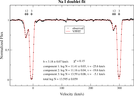
Figure 8: Na I $\lambda\lambda$5890, 5896 absorption in the Galaxy as seen toward SN 2000cx. The velocity scale is heliocentric, and centered on the $\lambda$5890 component. The galactic absorption is dominated by a component at $\sim-5\rm~{}km~{}s^{-1}$. There is also weaker blueshifted absorption around $20-25\rm~{}km~{}s^{-1}$, and the absorption can be traced on the blue side to $\sim-40\rm~{}km~{}s^{-1}$. Our VPFIT models disentangle three components. Their velocities and corresponding Na I column densities are shown in the figure, as well as in Table 3.

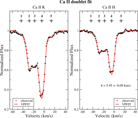
Figure 9: Ca II $\lambda\lambda$3933, 3968 absorption in the Galaxy as seen toward SN 2000cx. The velocity scale is heliocentric. Note that the galactic absorption is dominated by the same component around $-5\rm~{}km~{}s^{-1}$ as in Fig. 3, but that there are two more components than for Na I. For Ca II we identify the following components: $-43.4\pm 0.6$, $-28.1\pm 0.3$, $-18.0\pm 0.3$, $-4.6\pm 0.1$ and $13.4\pm 0.3\rm~{}km~{}s^{-1}$. The column densities for these components are given in Table 3. Components ‘2’, ‘3’ and ‘4’ (as marked in the figure) agree in velocity with the three Na I components in Fig. 8.

Figure 10: Weak Ca II H ($\lambda$3968, dashed) and K ($\lambda$3934, solid) absorption can also be seen from the host galaxy of SN 2000cx with maximum absorption at $2526.4\pm 0.3\rm~{}km~{}s^{-1}$, which is $147\rm~{}km~{}s^{-1}$ higher than the NED value for NGC 524. The Ca II column density in the host galaxy is $(5.5\pm 0.4)\times 10^{10}\rm~{}cm^{-2}$. No absorption due to Na I is seen from NGC 524. The velocity scale is heliocentric.

Table 3: Galactic interstellar absorption components toward SN 2000cx.

Line	velocitya	log(column density)
	(km s-1)	(cm-2)
Na I D	$-25.6\pm 0.3$	$11.41\pm 0.03$
	$-19.6\pm 0.3$	$11.16\pm 0.04$
	$-5.1\pm 0.1$	$13.59\pm 0.06$
Ca II H&K	$-43.4\pm 0.6$	$10.93\pm 0.04$
	$-28.1\pm 0.3$	$11.91\pm 0.01$
	$-18.0\pm 0.3$	$11.85\pm 0.01$
	$-4.6\pm 0.1$	$12.33\pm 0.01$
	$+13.4\pm 0.3$	$11.09\pm 0.03$

^aHeliocentric velocity.

3.1.3 Interstellar lines and reddening

The estimates in Table 2 did not take into account any reddening. The galactic reddening in the direction of NGC 524 is $E(B-V)=0.083$ (Schlegel et al. 1998). Burstein & Heiles (1982) found a lower value of $E(B-V)=0.03$ based on an H I/galaxy counts method. We have also estimated the amount of reddening from the Na I D absorption lines in our data. We have done this for epoch 2 when the supernova was brighter. The galactic Na I D lines at 5889.95 Å and 5895.92 Å have EWs of 0.36 Å and 0.29 Å, respectively, which is similar to what Patat et al. (2007a) find. As shown in Fig. 8, the lines seem to be made up of two major components, with the most redshifted being the strongest. No Na I D absorption at the velocity of NGC 524 could be detected. The pixel-to-pixel noise indicates an upper limit of an unresolved line of 4.2 mÅ, which shows that the extinction in the supernova host galaxy is indeed very low. Patat et al. (2007a) estimate an EW of $\!\!\!\phantom{\leq}\smash{\buildrel\over{\lower 2.67502pt\hbox{$\buildrel\lower 2.14001pt\hbox{$\displaystyle<$}\over{\sim}$}}}\,\,1$mÅ.

Also galactic absorptions in Ca II H and K are clearly present. The EW of Ca II K (3933 Å) is 0.23 Å and of Ca II H (3968 Å) 0.14 Å, again in perfect agreement with Patat et al. (2007a). The Ca II H absorption line profile (from our 25 July spectrum) is shown in Fig. 9. It is clear that the same red component at $-5\rm~{}km~{}s^{-1}$ as for Na I D also dominates Ca II, but that the bluer components ($-18\rm~{}km~{}s^{-1}$ and $-28\rm~{}km~{}s^{-1}$) are stronger and bracket the blue component of Na I D (cf. Fig. 8). However, if we allow the blue Na I component to be split up in two subfeatures using the program VPFIT (see Sollerman et al. 2005 for our use of VPFIT) as indicated in Fig. 8, their velocities coincide rather well with components of Ca II. Unlike Na I, Ca II has also absorption components at $\sim-43\rm~{}km~{}s^{-1}$ and $\sim+16\rm~{}km~{}s^{-1}$. The galactic components we identify using VPFIT, and their corresponding column densities are listed in Table 3 for both Na I and Ca II. The VPFIT models were made to fit both components of Na I simultaneously, and likewise the Ca II H & K components simultaneously. The different velocity components for each ion were assumed to have the same FWHM (the parameter $b$ in Figs. 8 and 9), which should be close to the instrumental resolution. Patat et al. (2007a) argue for a split of our $-4.6\pm 0.1\rm~{}km~{}s^{-1}$ component into two components, and an extra component at $-23.1\pm 0.1\rm~{}km~{}s^{-1}$, but do not identify our component at $-43.4\pm 0.6\rm~{}km~{}s^{-1}$.

Figure 11: VLT/FORS2 spectrum of SN 2000cx at 363 days after $B$ maximum. The overall spectrum is described in Sollerman et al. (2004). The inset shows a detailed view of the region marked by dashed lines, concentrating on wavelengths around H$\alpha$, i.e., $\sim 6615$ Å at the redshift of the supernova. The dashed and dotted spectra in the inset are models for the supernova, assuming 0.01 and 0.05$~{}{\rm M}_{\odot}$ of solar abundance material, respectively, concentrated to $\pm 10^{3}\rm~{}km~{}s^{-1}$ around the recession velocity of the supernova. This is to simulate H$\alpha$ emission from gas removed from a possible companion star according to the models of Marietta et al. (2000). Our models for the H$\alpha$ emission are described in the text. There is no sign of H$\alpha$ emission in SN 2000cx at these wavelengths, which places a limit on hydrogen-rich material at velocities below $10^{3}\rm~{}km~{}s^{-1}$ of $\sim 0.03~{}{\rm M}_{\odot}$.

Figure 12: VLT/FORS1 spectrum of SN 1998bu at 388 days after $B$-band maximum. The overall spectrum is described in Spyromilio et al. (2004). The inset is a blow-up of the region marked by dashed lines, concentrating on wavelengths around H$\alpha$. As in Fig. 11 we have plotted our model for H$\alpha$ emission from a possible ablated companion star, and the mass within the core (i.e., $\pm 10^{3}\rm~{}km~{}s^{-1}$) is the same as in Fig. 11. We have assumed a distance to SN 1998bu of 11.2 Mpc, an extinction of A${}_{V}=1.0$ and a redshift of $750\rm~{}km~{}s^{-1}$ (Munari et al. 1998; Centurion et al. 1998). There is no sign of H$\alpha$ emission in SN 1998bu at the expected wavelength.

Although much fainter, the Ca II H and K lines are also detected in NGC 524 (Fig. 10). The EW of the host galaxy lines are about 2.9 and 1.5mÅ, respectively, i.e., roughly 100 times weaker than the Galactic lines. The redshift of these lines correponds to a velocity of 2526 km s^-1, which is 147 (or 173) km s^-1 higher than the recession velocity of NGC 524 according to NED (or Emsellem et al. 2004). This may be due to the rotation of NGC 524 at the position of the absorbing gas. Using VPFIT, the Ca II column density in NGC 524 toward the supernova is a mere $(5.5\pm 0.4)\times 10^{10}\rm~{}cm^{-2}$. This low value is not surprising given the galaxy type of NGC 524 (S0). Patat et al. (2007a) find a column density of $(4.4\pm 0.5)\times 10^{10}\rm~{}cm^{-2}$, i.e., consistent with our value, as well as only $3\rm~{}km~{}s^{-1}$ difference in recession velocity.

We have used our EWs in combination with the expressions of Munari & Zwitter (1997) to estimate the amount of Galactic reddening in the direction of the supernova. According to their Table 2, an EW of 0.36 Å in Na I correponds to $E(B-V)\simeq 0.15$, i.e., higher than the NED value given by Schlegel at al. (1998). However, as illustrated in Figs. 8 and 9, and in Table 3, the interstellar absorption toward SN 2000cx is composed of at least three components which means that there is no simple relation between $E(B-V)$ and Na I column density. In particular, for a saturated line like the central component of the Na I D lines in our data, the EW scales roughly as $\propto$ lg($N_{\rm col}$), whereas adding unsaturated components outside the core of the saturated one makes the EW scale with the total column density as $\propto N_{\rm col}$. Added to this uncertainty due to the cloud distribution, the EW vs. $E(B-V)$ relation is also sensitive to the degree of ionization along the line of sight to the supernova, as well as to the gas-to-dust ratio. With these caveats in mind, Na I D absorption can therefore, at best, only provide a rough estimate of the extinction. We have discussed this further for SN 2001el in Sollerman et al. (2005).

A further constraint on the extinction of SN 2000cx comes from the supernova itself. In Li et al. (2001), the late time color of SN 2000cx is shown to be very blue. When corrected for a Galactic extinction of $E(B-V)=0.15$, it is indeed bluer than for most known unreddened SNe Ia. This argues that the extinction is low toward SN 2000cx, and that the Na I D absorption could give too high an estimate of $E(B-V)$ using the simple Munari & Zwitter approach. As mentioned in Sect. 3.1.1, the likely DIB feature at 6613.56 Å provides an estimate of $E(B-V)$, and we found $E(B-V)\sim 0.1$, which would support the Schlegel et al. galactic reddening estimator. It should be cautioned that the scatter on the EW/$E(B-V)$ relation for the DIB could easily be 50%, and possibly even a factor 2, in particular for very low reddening sightlines. However, as there seems to be no strong evidence against using the Schlegel et al. estimate of $E(B-V)=0.08$, we have in the following used this value. This yields a flux correction factor of 1.20 for H$\alpha$, 1.23 for He I $\lambda$5876, and 1.32 for He II $\lambda$4686 for the limits obtained for the circumstellar emission in Sect. 2.1.2.

3.1.4 FORS observations and data reductions

On 2001 July 24 we obtained a 2400 s exposure using FORS2 on UT4. We used the 300V grism together with order sorting filter GG375 and a $1\aas@@fstack{\prime\prime}3$ wide slit. Two nights later, on 2001 July 26, this spectrum was complemented with another 2400 s exposure with the 300I grism and the OG590 filter. Together these two spectra cover the wavelength region $\sim 3700-9200$ Å.

The spectra were reduced in a standard way, including bias subtraction, flat fielding and wavelength calibration using exposures of a Helium-Argon lamp. Flux calibration was done relative to the spectrophotometric standard star LTT377 in 300V and to G158-100 in 300I. The absolute flux calibration of the combined spectrum was also checked against broad band photometry of the SN.

3.1.5 Late emission

In Fig. 11 we show the combined optical spectrum (2001 July 24 and 26) of SN 2000cx. The average epoch corresponds to day 363 after maximum. The general features of the spectrum are discussed in Sollerman et al. (2004) along with the late photometry of the supernova. Here we use the spectrum for an inspection of possible signatures of gas from a tentative hydrogen-rich binary companion, as described in the models of Marietta et al. (2000). The inset shows a detailed view of the spectral region around H$\alpha$, along with our model calculations discussed in Sect. 2.2. We see no evidence of emission from gas originating from a companion.

3.2 SN 1998bu

3.2.1 FORS observations and data reductions

We have also made a similar test for our late spectra of SN 1998bu. The supernova was observed using FORS1 on VLT on 1999 June 11 corresponding to 388 days past maximum. These observations and data reductions are described in Spyromilio et al. (2004).

As shown by Cappellaro et al. (2001), SN 1998bu started to deviate from the normal SN Ia decay rate some time after $\sim 300$ days, and by $\sim 500$ days it was brighter by $\sim 2$ magnitudes than normal SNe Ia (e.g., SN 1996X). The reason for this is that SN 1998bu was strongly affected by a light echo. The magnitude we estimate on day 388 places SN 1998bu less than half a magnitude (in $V$-band) from the “light echo free” $V$-band light curve shown in Fig. 1 of Cappellaro et al. (2001). This means that the observation at 388 days is the latest phase available (see also Spyromilio et al. 2004) for SN 1998bu, while still rather unaffected by the light echo.

Figure 13: Infrared spectra of SN 1998bu in the nebular phase taken at 251 days (ESO/NTT/SOFI) and 346 days (ESO/VLT/ISAAC) after $B$ maximum. The overall spectra are modeled and discussed in Spyromilio et al. (2004). The day 251 spectrum has been shifted upwards by $10^{-17}$ erg s^-1 cm^-2Å^-1 for clarity, and its zero-level is marked by a dashed line. The arrows mark the rest wavelenghts of Pa$\alpha$ and Pa$\beta$ for SN 1998bu. The insets show blow-ups of the spectral region around Pa$\alpha$. The dashed line shows a model discussed in Sect. 2.2 and displayed in Fig. 13 assuming $0.5~{}{\rm M}_{\odot}$ of hydrogen-rich material within the innermost $\pm 10^{3}\rm~{}km~{}s^{-1}$ of the ejecta. This is to simulate the emission from the companion star in the models of Marietta et al. (2000). However, there is no sign of such Pa$\alpha$ emission in SN 1998bu. Note that Pa$\alpha$ sits in a region of very poor atmospheric transmission, and that Pa$\beta$ is a less efficient emitter and sits in the wing of a strong ejecta line (see Spyromilio et al. 2004). The modeled emission in the inset of the lower spectrum was shifted upwards by $5\times 10^{-18}$ erg s^-1 cm^-2Å^-1 to overlap with the observed spectrum. Same reddening, redshift and distance were assumed as in Fig. 12.

The resulting spectrum is shown in Fig. 12 (see also Fig. 4 of Spyromilio et al. 2004), and it is indeed very similar to the nebular spectrum at 330 days published by Cappellaro et al. (2001). A more careful inspection shows that the emission blueward of $\sim 4500$Å is relatively stronger in our day 388 spectrum, which is likely to be a sign of the light echo, as also highlighted in Fig. 4 of Spyromilio et al. (2004). Of more importance to the current analysis is the region around H$\alpha$ at the expected redshift of SN 1998bu. We have also included the results from the model calculations discussed in Sect. 2.2 for the H$\alpha$ emission expected in the models of Marietta et al. (2000) if hydrogen is evaporated off a companion star. We find no sign of H$\alpha$ emission within this interval.

3.2.2 NTT/SOFI and VLT/ISAAC observations

We have also observed SN 1998bu in the infrared 251 days and 346 days after $B$ maximum with NTT/SOFI and VLT/ISAAC, respectively. Both these spectra (shown in Fig. 13) are safely within the nebular phase, and should be unaffected by the light echo. While Spyromilio et al. (2004) describe details of the observations, and also model the supernova emission, we concentrate here on the $\pm 10^{3}\rm~{}km~{}s^{-1}$ velocity intervals around the expected wavelengths of Pa$\alpha$ and Pa$\beta$ for the same reason as we did for H$\alpha$ in Sect. 3.2.1.

To obtain a better signal-to-noise we have binned the spectrum in 20Å bins, corresponding to $\sim 320\rm~{}km~{}s^{-1}$ at Pa$\alpha$. As for H$\alpha$ in Sect. 3.2.1, we see no evidence of material from a companion star. The test in the infrared is, however, more complicated since Pa$\alpha$ sits in a region of very poor atmospheric transmission, and Pa$\beta$ is expected to be a less efficient emitter and sits in the wing of a strong ejecta line (see Spyromilio et al. 2004) which may have intrinsic structures that could confuse the search for $\!\!\!\phantom{\leq}\smash{\buildrel\over{\lower 2.67502pt\hbox{$\buildrel\lower 2.14001pt\hbox{$\displaystyle<$}\over{\sim}$}}}\,\,10^{3}\rm~{}km~{}s^{-1}$ Pa$\beta$ emission.

3.3 Early Ca II absorption

As discussed in Sect. 1 several SN Ia show high-velocity (HV) absorption features in the Ca II IR and H&K lines. For the particular case of SN 2000cx, Thomas et al. (2004) identified in the +2 day spectrum of Li et al. (2001) HV features in both the IR and H&K lines. While the IR triplet have several subfeatures, the H&K feature is wide and flat. The velocity of the absorptions reaches out to $\sim 2.4\times 10^{4}\rm~{}km~{}s^{-1}$ and $\sim 2.2\times 10^{4}\rm~{}km~{}s^{-1}$, if we refer to the bluest components of the multiplets, i.e., to $\lambda 3934$ and $\lambda 8498$Å, respectively, and adopt a recession velocity of $v_{rec}$ = 2379 km s^-1 for the supernova. Any changes in these velocities with time (up to +7 days) are difficult to disentangle from the data presented in Thomas et al. (2004), although there may be a hint that at least the IR feature may recede marginally.

Thomas et al. (2004) modelled the HV features assuming both spherical and nonspherical distributions of the absorbing material. Their best fit was obtained assuming both spherical symmetry and an elongated feature along the line of sight with a maximum optical depth at $2.24\times 10^{4}\rm~{}km~{}s^{-1}$ (cf. their Fig. 9). Interestingly enough, Leonard et al. (2000) reported continuum polarization of $\sim 0.5\%$ for this supernova at +2 days, which could in fact signal an aspherical scattering surface.

We have used our data to extend the study of HV Ca II absorption in SN 2000cx to $-6$ days. As for our data of SN 2001el presented in M05 we decided to normalize the continuum by a first order polynomial fit around the profile of interest to better trace the line wings. The normalized spectra are shown in Fig. 14 where the solid line is for the IR triplet, and the dashed line for the H&K lines. The velocities are with respect to the bluest components of the multiplets as discussed for the data of Thomas et al. (2004) above.

Figure 14: Comparison between the Ca II IR triplet (solid line) and the Ca II H$\&$K lines (dashed line) at $-6$ days. The flux calibrated ($f_{\lambda}$) spectral features have been normalized and converted to velocity space w.r.t. to the rest wavelengths assuming $v_{rec}$ = 2379 km s^-1 for SN 2000cx. For this we used the rest wavelengths of the bluest components of the Ca II triplet/doublet lines viz. 3934 Å and 8498 Å.

For the H&K lines we find that the Ca II absorption reaches out to $\sim 2.4\times 10^{4}\rm~{}km~{}s^{-1}$, and for IR lines at least out to $\sim 2.2\times 10^{4}\rm~{}km~{}s^{-1}$. There is also an absorption feature in the IR lines reaching $\sim 2.8\times 10^{4}\rm~{}km~{}s^{-1}$ which, however, does not appear to be present in the H&K lines. Furthermore, it can be expected that the H&K lines have a higher optical depth (e.g., Mihalas 1978) and are present at a higher velocity than the IR lines as they originate from a lower level of the Ca II ion and have larger oscillator strengths. In fact, the HV H&K lines have been observed to show wings extending to much higher velocities than the IR lines at least in SNe 1990N and 2001el (for details see M05). However, this behavior could also be due to the H&K profile blending with other lines (e.g., Kasen et al. 2003), and therefore a full NLTE analysis would be needed to be conclusive for SN 2000cx. Also, the Ca II line absorption shown by SN 2000cx is much weaker than the one seen in SNe 1990N and 2001el, making an estimate of the maximum velocity less accurate.

In contrast to the behavior shown by, e.g., SN 2001el (M05), it appears that in SN 2000cx the maximum Ca II velocities at $-6$ days are similar to the maximum velocites at $+2$ days. In general, a decreasing maximum velocity of the Ca II absorption would be expected simply because the column density of the ejecta decreases with time as $\propto t^{-2}$, and disregarding abundance and ionization effects, the most dilute gas will become optically thin faster. For the outer ejecta, the density falls off quickly with radius (cf. Sect. 3.1) so a receding blue edge of the IR triplet could fit into a picture where the outermost ejecta become progressively optically thinner in Ca II. The constant maximum Ca II velocity of SN 2000cx could indicate that the structure of the absorbing gas is more shell-like than in SN 2001el, although we reiterate that conclusions from the weaker absorption in SN 2000cx must be drawn with caution.

4 Discussion and Summary

4.1 Limit on wind density from absence of circumstellar line emission

In Section 3.1.2 we derived upper limits for the H$\alpha$ line fluxes (see Table 2). Adopting an extinction of $E(B-V)$=0.08 and a distance of 33 Mpc for SN2000cx, these flux limits correspond to line luminosities of $L_{\rm H\alpha}$ = 1.3, 2.1, 2.4, and 3.7 $\times$ 10³⁷ erg s^-1 for the first epoch observation and wind speed of 10, 50, 100, and 200 $\rm~{}km~{}s^{-1}$, respectively. For the second and third epoch observations, respectively, the upper limits for a 10 $\rm~{}km~{}s^{-1}$ wind are 1.4 and 0.50 $\times$ 10³⁷ erg s^-1, and for a 50 $\rm~{}km~{}s^{-1}$ wind they are 2.2 and 0.77 $\times$ 10³⁷ erg s^-1. For the fourth epoch observations our upper limits correspond to $L_{\rm H\alpha}$ = 2.1, 2.7, 3.2, and 4.8 $\times$ 10³⁶ erg s^-1 for the wind speeds of 10, 50, 100, and 200 $\rm~{}km~{}s^{-1}$, respectively. In these estimates we have assumed a luminosity-weighted temperature of H$\alpha$ emitting gas of $2.8\times 10^{4}$ K. From Fig. 2 one can see that this is a reasonable assumption since the temperature remains within $2.2\times 10^{4}-3.4\times 10^{4}$ K for all our $T_{e}=T_{i}$ models after $\sim 6$ days. The difference is small for models with $T_{e}=T_{rev}/2$. Table 2 also gives upper limits for He I $\lambda 5876$ and He II $\lambda 4686$ for the first two epochs using the same luminosity-weighted temperature. For the He II line, this temperature is an underestimate, but as discussed below, this does not affect our conclusions.

Figure 3 shows that for the earliest epoch, the limit on $\dot{M}/v_{w}$ from H$\alpha$ for a normal He/H abundance of the CSM and $v_{w10}=1$ is $\sim 1.5\times 10^{-5}~{}{\rm M}_{\odot}~{}{\rm yr}^{-1}$. Should the wind be more helium-rich or faster, we cannot place any limit on $\dot{M}$, neither from H$\alpha$ nor He I $\lambda 5876$ and He II $\lambda 4686$, although the latter line comes close to the detection limit for $\dot{M}\sim 2\times 10^{-5}v_{w10}^{-1}~{}{\rm M}_{\odot}~{}{\rm yr}^{-1}$ for $\rm{He/H}=1$ and $v_{w10}=1$. An even more promising helium-line to look for seems to be He I $\lambda 10\,830$. This line could, however, not be covered by the UVES observations.

Turning to the later epochs, we note no improvement in terms of the limit on $\dot{M}$ from H$\alpha$, except for 85 days post explosion, for which we find the limit $\sim 1.3\times 10^{-5}~{}{\rm M}_{\odot}~{}{\rm yr}^{-1}$ in case of $\rm{He/H}=0.085$ and $v_{w10}=1$. For $v_{w10}=5$ (and $\rm{He/H}=0.085$), the limit goes up $\dot{M}\sim 7.5\times 10^{-5}~{}{\rm M}_{\odot}~{}{\rm yr}^{-1}$, and for still higher $\dot{M}$ the limit goes beyond $10^{-4}~{}{\rm M}_{\odot}~{}{\rm yr}^{-1}$. For $\rm{He/H}=0.3$ and $v_{w10}=1$ the limit is $\dot{M}\sim 1.8\times 10^{-5}~{}{\rm M}_{\odot}~{}{\rm yr}^{-1}$. In the most favorable case of our models, the limit on $\dot{M}$ is thus $\sim 1.3\times 10^{-5}~{}{\rm M}_{\odot}~{}{\rm yr}^{-1}$ (for a normal He/H-ratio as well as slow wind ($v_{w10}=1$). A more helium-rich wind degrades the limit somewhat, whereas a faster wind moves the limit on $\dot{M}$ upwards quickly. The limit is also prone to systematic uncertainties, in particular the assumptions for the ionizing spectrum, as well as the assumption of a smooth, spherically distribution of the CSM. How these effects affect the limit of $\dot{M}$ was discussed in some detail in C96.

4.2 Comparing our circumstellar limits for SN 2000cx to other supernovae

We have looked for narrow hydrogen and helium lines in our early high-resolution optical spectra of the Type Ia supernova SN 2000cx. No such lines were detected. We have made detailed time dependent photoionization models for the possible circumstellar matter to interpret these non-detections. The best limit was obtained from H$\alpha$, and we put a limit on the mass loss rate from the progenitor system of $\sim 1.3\times 10^{-5}~{}{\rm M}_{\odot}~{}{\rm yr}^{-1}$ in case of $\rm{He/H}=0.085$ and $v_{w10}=1$, where $v_{w10}$ is the wind speed in $10\rm~{}km~{}s^{-1}$. These limits are sensitive to gas outside a few $\times 10^{15}$ cm from the supernova. Possible circumstellar matter closer to the supernova would have been swept up before our observations. The limit is slightly higher than that we found for SN 2001el (M05) for which we derived $\sim 9\times 10^{-6}~{}{\rm M}_{\odot}~{}{\rm yr}^{-1}$, but similar to what C96 found for SN 1994D. However, the model for SN 1994D assumed a much slower circumstellar shock and applying the model used in this paper to the Cumming et al. study of SN 1994D would increase their limit substantially.

The H$\alpha$ based upper limits on circumstellar matter around SNe Ia described in M05 for SN 2001el and here for SN 2000cx are the most sensitive so far. These results, together with the previous observational work on SN 1994D (C96) disfavour a symbiotic star in the upper mass loss rate regime (so called Mira type systems) from being the likely progenitor scenario for these SNe. This is in accordance with the models of Hachisu et al. (1999a, 1999b), which do not indicate a mass loss rate of the binary companion in the symbiotic scenario higher than $\sim$10^-6 $~{}{\rm M}_{\odot}~{}{\rm yr}^{-1}$. Stronger mass loss would initiate a powerful (although dilute) wind from the white dwarf that would clear the surroundings of the white dwarf, and that may even strip off some of the envelope of the companion. The white dwarf wind with its possible stripping effect, in combination with the orbital motion of the stars, is likely to create an asymmetric CSM. Effects of a more disk-like structure of the denser parts of the CSM, and how this connects to our spherically symmetric models, are discussed by C96 In general, lower values of $\dot{M}/V_{\rm wind}$ should be possible to trace in an asymmetric scenario, although uncertainties due the inclination angle and the flatness of the dense part of the CSM would also be introduced. However, to push the upper limits down to the $\sim$ 10^-6 $~{}{\rm M}_{\odot}~{}{\rm yr}^{-1}$ level a much more nearby ($D\sim 5$ Mpc) SN Ia needs to be observed even earlier ($\sim 15$ days before the maximum light) than our first epoch observation of SN 2001el (M05).

Similar, or even lower limits on $\dot{M}/V_{\rm wind}$ can be obtained from X-ray, and especially radio observations (e.g., Eck et al. 2002), but such observations cannot disentangle the elemental composition of the gas in the same direct way as optical observations can do. The most constraining radio limit so far is that of $\sim$ 10^-9 $~{}{\rm M}_{\odot}~{}{\rm yr}^{-1}$ for the nearby SN 2011fe (Chomiuk et al. 2012) which essentially rules out all likely single degenerate progenitor systems. One should, however, keep in mind that also SN 2006X was radio silent, which was used by Chugai (2008) to argue for a mass loss rate below $\sim$ 10^-8 $~{}{\rm M}_{\odot}~{}{\rm yr}^{-1}$ for the progenitor system for that supernova, despite it possibly having circumstellar gas (Patat et al. 2007b). The main problem with X-rays and radio limits, as well as the method used in this paper, is that they probe circumstellar gas through ongoing shock interaction. Circumstellar gas in shell-like structures far away from the explosion site are better probed by the absorption-line method (e.g., Patat et al. 2007b), though a disk-like CSM may be missed if the line-of-sight is not in the disk plane. For nearby SNe Ia it seems imperative that both high-resolution spectroscopy as early as possible and up to the first $\sim 100$ days should be performed, as well as continued radio monitoring for several years. SN 2011fe may provide a good testbed for such investigations. Somewhat discouraging for the latter is that no SNe Ia has been detected in radio, despite many of them having been nearby, as well as observed over a range of times since explosion (Eck et al. 2002). For example, SN 1937C and SN 1972A did not show any radio emission at ages 48.7 and $9.0-13.7$ years, respectively. It could be that circumstellar shells in some cases are so far out that one has to wait until the remnant phase to see increased shock interaction (Chiotellis et al. 2012). The obvious exceptions are members of the SN 2002ic like supernovae. A particularly interesting case is PTF 11kx (Dilday et al. 2012) with its circumstellar interaction turning on after maximum light. For this case, inverse Compton scattering in the shocked gas should be less important than if interaction would have started immediately after the explosion. Our models should therefore be applicable to this supernova after the circumstellar shock had formed.

4.3 Limit on hydrogen-rich gas from a companion

In the insets of Figs. 11 and 12, models with $0.01~{}{\rm M}_{\odot}$ and $0.05~{}{\rm M}_{\odot}$ were compared with late time spectra of SNe 2000cx and 1998bu, respectively. From these insets it is obvious that $0.05~{}{\rm M}_{\odot}$ of solar abundance material with a velocity of $\!\!\!\phantom{\leq}\smash{\buildrel\over{\lower 2.67502pt\hbox{$\buildrel\lower 2.14001pt\hbox{$\displaystyle<$}\over{\sim}$}}}\,\,10^{3}\rm~{}km~{}s^{-1}$ should have been seen in both SN 1998bu and SN 2000cx. Our calculations give a lower limit on the amount of solar abundance material of $\sim 0.03~{}{\rm M}_{\odot}$ that would not escape detection in late H$\alpha$ spectra of the two supernovae. A similar limit was obtained by M05 for the late emission of SN 2001el, and Leonard (2007) finds $\sim 0.01~{}{\rm M}_{\odot}$ for SNe 2005am and 2005cf using our models. As discussed in M05, the limits we obtain for the $\!\!\!\phantom{\leq}\smash{\buildrel\over{\lower 2.67502pt\hbox{$\buildrel\lower 2.14001pt\hbox{$\displaystyle<$}\over{\sim}$}}}\,\,10^{3}\rm~{}km~{}s^{-1}$ solar abundance material in all those five supernovae should be conservative limits. The limit on SN 2011fe by Shappee et al. (2013b) is even lower, $0.001~{}{\rm M}_{\odot}$, and rests on an extrapolation of our model simulations to masses below $0.01~{}{\rm M}_{\odot}$.

Figure 13 shows that the infrared spectrum of SN 1998bu would not reveal even $0.50~{}{\rm M}_{\odot}$ of hydrogen-rich gas at those wavelengths. Pa$\alpha$ (or Pa$\beta$) based limits on hydrogen-rich gas are therefore substantially higher than for H$\alpha$ (cf. Fig. 12), even with the most powerful instruments presently available. However, future space missions such as the James Webb Space Telescope (JWST) could provide a powerful tool to detect Pa$\alpha$.

Comparing a $\sim$0.01-0.03 M_⊙ limit to the numerical simulations of Marietta et al. (2000) indicates that symbiotic systems with a subgiant, red giant or a main-sequence secondary star at a small binary separation are not likely progenitor scenarios for these SNe. More recent modeling by Pakmor et al. (2008) shows that the material stripped by the companion could be significantly lower than that estimated by Marietta et al. (2000). In one of the six models for main-sequence donors tested by Pakmor et al. (2008), the mass of stripped envelope was even lower than the $\!\!\!\phantom{\leq}\smash{\buildrel\over{\lower 2.67502pt\hbox{$\buildrel\lower 2.14001pt\hbox{$\displaystyle<$}\over{\sim}$}}}\,\,$0.01_⊙ limit of Leonard (2007). On the other hand, the most recent models (Pan et al. 2012) have again pushed the evaporated mass for hydrogen-rich donors up to levels surpassing our limits.

A solution to any conflict between the ablated mass in impact models and our limits on hydrogen in the nebular phase could be twofold: either the separation between the companions is large, or the donor star is a helium-rich star. (See Fig. 12 of Pan et al. 2012, which summarizes the yield of unbound masses in models made so far.) It is, however, not only the ablated mass that is important, but also the velocity distribution of this material. In our models we have distributed the material evenly within a $1000\rm~{}km~{}s^{-1}$ sphere. A velocity much below $1000\rm~{}km~{}s^{-1}$ would push our limits down to below $\sim$0.01 M_⊙. Pan et al. (2012) shows that most of the mass lost has indeed velocities below $1000\rm~{}km~{}s^{-1}$, peaking at $\sim 500-600\rm~{}km~{}s^{-1}$ in the case of a hydrogen-rich donor. Helium-rich companions, on the other hand, have velocities which peak in velocity around $1000\rm~{}km~{}s^{-1}$. In the helium-rich case, the ablated mass is in most models below 0.01 M_⊙, and the observational signature would obviously in this case not be hydrogen lines, but lines from other elements. Figure 5 shows that lines from O I and Ca II are promising probes. There is also the possibility that all the five SNe Ia with a maximum of $\sim$0.01-0.03 M_⊙ hydrogen-rich gas, like very likely SN 2011fe (Shappee et al. 2013b), stem from double degenerate systems. One issue that is not a matter of concern in our models is radiative transfer effects of any H$\alpha$ emission produced in the center of our SN Ia models. In all cases, the H$\alpha$ emission emerges unattenuated, i.e., electron scattering and line transfer are unimportant. To make even more accurate predictions of possible hydrogen/helium line emission we should use nebular emission models with a larger line list to test this, in conjunction with hydro simulations like those of Pan et al. (2012). At the same time, further deep spectra of SNe Ia in the nebular phase are needed to get better supernova statistics. Comparing with Fig. 12 of Pan et al. (2012), it seems hydrogen-rich donors with a separation of $\!\!\!\phantom{\leq}\smash{\buildrel\over{\lower 2.67502pt\hbox{$\buildrel\lower 2.14001pt\hbox{$\displaystyle<$}\over{\sim}$}}}\,\,$5 times the radius of the donor may be ruled out for the in total five SNe discussed here, by M05 and by Leonard (2007). For SN 2011fe one has very likely to resort to a double degenerate scenario.

We thank Sergei Blinnikov and Elena Sorokina for discussions, and for making the models w7jz.ph and w7jzl155.ph available to us. This work was supported by the Swedish Research Council, the Swedish Space Board, and the Royal Swedish Academy of Sciences. We also thank the staff at Paranal for carrying out the service observations of SN 2000cx. PL acknowledges support the Wallenberg Foundation and the Kavli Institute of Theoretical Astrophysics where part of this work was done. SM acknowledges support from the EC Programme ‘The Physics of Type Ia SNe’ (HPRN-CT-2002-00303; PI: W. Hillebrandt) and from the Participating Organisations of EURYI and the EC Sixth Framework Programe. JS acknowledges a Reserach Fellowship at the Royal Swedish Academy supported by a grant from the Wallenberg Foundation. EB was supported in part by grants from DOE, NASA and the NSF.

References

- [Aldering (2006)] Aldering, G. 2006, ApJ, 650, 510
- [Benetti et al.(2006)] Benetti, S., Cappellaro, E., Turatto, M., Taubenberger, S., Harutyunyan, A., & Valenti, S. 2006, ApJL, 653, L129
- [Benz et al. 1990] Benz, W., Cameron, A. G. W., Press, W. H., & Bowers, R. L. 1990, ApJ, 348, 647
- [Blinnikov & Sorokina 2000] Blinnikov, S. I., & Sorokina, E. 2000, A&A, 356, L30
- [Blinnikov & Sorokina 2001] Blinnikov, S. I., & Sorokina, E. I. 2001, in Scientific prospects of the space ultraviolet observatory SPECTRUM-UV, ed. B. M. Shustov & D. S. Wiebe (Moscow: GEOS) (in Russian), 84
- [Branch 1998] Branch, D. 1998, ARA&A, 36, 17
- [Branch et al. 1985] Branch, D., Doggett, J. B., Nomoto, K., & Thielemann, F.-K. 1985, ApJ, 294, 619
- [Branch et al. 1995] Branch, D., Livio, M., Yungelson, L. R., Boffi, F. R., & Baron, E. 1995, PASP, 107, 1019
- [Branch et al.(2004)] Branch, D. et al. 2004, ApJ, 606, 413
- [Burstein & Heiles 1982] Burstein, D., & Heiles, C. 1982, AJ, 87, 1165
- [Cappellaro et al. 2001] Cappellaro, E. et al., 2001, ApJ, 549, 215
- [Centurion et al. 1998] Centurion, M., Walton, N., & King, D. 1998, IAU Circ., 6918
- [Chandra et al. 2008] Chandra, P., Chevalier, R., & Patat, F. 2008, ATel, 1391, 1
- [Chevalier 1982a] Chevalier, R. A. 1982a, ApJ, 258, 790
- [Chevalier 1982b] Chevalier, R. A. 1982b, ApJ, 259, 302
- [Chiotellis 2012] Chiotellis, A., Schure, K. M., & Vink J. 2012, A&A, 537, 139
- [Chomiuk et al.(2012)] Chomiuk, L., Soderberg, A. M., Moe, M., et al. 2012, ApJ, 750, 164
- [Chornock et al. 2000] Chornock, R. et al. 2000, IAU Circ., 7463
- [Chugai (2008)] Chugai, N. 2008, Astronomy Letters, 34, 389
- [Chugai et al. 2004] Chugai, N. N., Chevalier, R. A., & Lundqvist, P. 2004, MNRAS, 355, 627
- [Chugai & Yungelson (2004)] Chugai, N. N., & Yungelson, L. R. 2004, Astr. Letters, 30, 65
- [Crotts & Yourdon(2008)] Crotts, A. P. S., & Yourdon, D. 2008, ApJ, 689, 1186
- [Cumming et al. 1996] Cumming, R. J., Lundqvist, P., Smith, L. J., Pettini, M., & King, D. L. 1996, MNRAS, 283, 1355 (C96)
- [Deng et al. (2004)] Deng, J., Kawabata, K. S., Ohyama, Y., Nomoto, K., Mazzali, P. A., Wang, L., Jeffery, D. J., Iye, M., Tomita, H., & Yoshii, Y. 2004, ApJ, 605, 37
- [Dilday et al.(2012)] Dilday, B., Howell, D. A., Cenko, S. B., et al. 2012, Science, 337, 942
- [Di Stefano et al. (2011)] Di Stefano, R., Voss, R., & Clayes, J. S. W. 2011, ApJ, 738, L1
- [D’Odorico & Kaper 2000] D’Odorico, S., & Kaper, L. 2000, UVES Users Manual
- [Dwarkadas & Chevalier 1998] Dwarkadas, V. V., & Chevalier, R. A. 1998, ApJ, 497, 807
- [Eck et al.(2002)] Eck, C. R., Cowan, J. J., & Branch, D. 2002, ApJ, 573, 306
- [Emsellem et al. 2004] Emsellem, E., Cappellari, M., Peletier, R. F. et al. 2004, MNRAS, 352, 721
- [Fransson 1984] Fransson, C. 1984, A&A, 133, 264
- [Fransson & Björnsson 1998] Fransson, C., & Björnsson, C.-I. 1998, ApJ, 509, 861
- [Fransson et al. 1996] Fransson, C., Lundqvist, P., & Chevalier R. A. 1996, ApJ, 461, 993
- [Gerardy et al. 2003] Gerardy, C. L. et al. 2003, ApJ, 607, 391
- [Hachisu et al.(1999a)] Hachisu, I., Kato, M., & Nomoto, K. 1999a, ApJ, 522, 487
- [Hachisu et al.(1999b)] Hachisu, I., Kato, M., Nomoto, K, & Umeda, H. 1999b, 519, 314
- [Hachisu et al.(2008)] Hachisu, I., Kato, M., & Nomoto, K. 2008, ApJ, 679, 1390
- [Hamuy et al.(2003)] Hamuy, M. et al., 2003, Nature, 424, 651
- [Han & Podsiadlowski (2003)] Han, Z., & Podsiadlowski, Ph. 2006, MNRAS, 368, 1095
- [Hillebrandt & Niemeyer 2000] Hillebrandt, W., & Niemeyer, J. 2000, ARA&A, 38, 191
- [Hoyle & Fowler 1960] Hoyle, F., & Fowler, W. A. 1960, ApJ, 132, 565
- [Hughes et al.(2007)] Hughes, J. P., Chugai, N., Chevalier, R., Lundqvist, P., & Schlegel, E. 2007, ApJ, 670, 1260
- [Iben & Renzini 1983] Iben, I. Jr., & Renzini, A. 1983, ARA&A, 21, 271
- [Iben & Tutukov] Iben, I. Jr. & Tutukov, A. V. 1984, ApJS, 54, 335
- [Justham (2011)] Justham, S. 2011, ApJ, 730, L34
- [Kasen(2010)] Kasen, D. 2010, ApJ, 708, 1025
- [Kasen et al.(2003)] Kasen, D. et al. 2003, ApJ, 593, 788
- [Kotak et al. 2004] Kotak, R., Meikle, W. P. S., Adamson, A., & Leggett, S. K. 2004, MNRAS, 354, L13
- [Kozma & Fransson 1998] Kozma, C., & Fransson, C.. 1998, ApJ, 496, 946
- [Kozma et al. 2005] Kozma, C., et. al. 2005, A&A, 437, 983
- [Leonard et al. 2000] Leonard, D. C., Filippenko, A. V., Chornock, R., & Li, W. D. 2000, IAU Circ., 7471
- [Leonard(2007)] Leonard, D. C. 2007, ApJ, 670, 1275
- [Li et al. 2001] Li, W. D. et al., 2001, PASP, 113, 1178
- [Li et al.(2001)] Li, W. et al. 2001, ApJ, 546, 734
- [Li et al.(2011)] Li, W., et al. 2011, Nature, 480, 348
- [Liu et al.(2012)] Liu, Z. W., Pakmor, R., Röpke, F. K., et al. 2012, A&A, 548, A2
- [Livio & Riess (2003)] Livio, M., & Riess, A. G. 2003, ApJ, 594, L93
- [Luna 2008] Luna, R., Cox, N. L. J., Satorre, M. A., Garcia Hernandez, D. A., Suarez, O. & Garcia Lario, P. 2008, A&A, 480, 133
- [Lundqvist & Cumming 1997] Lundqvist, P., & Cumming, R. J. 1997, in Advances in Stellar Evolution, ed. R. T. Rood & A. Renzini (CUP: Cambridge), 293 (LC97)
- [Lundqvist & Fransson (1996)] Lundqvist, P., & Fransson, C. 1996, ApJ, 464, 924
- [Lundqvist et al.(2005)] Lundqvist, P. et al. 2004, in Proceedings “Supernovae”, IAU Coll. 192, eds. J.M. Marcaide & K.W. Weiler (astro-ph/0309006), CDROM p. 81
- [Lundqvist et al.(2003)] Lundqvist, P. et al., 2003, in From Twilight to Highlight: The Physics of Supernovae, eds. W. Hillebrandt & B. Leibundgut, p. 309
- [Marietta et al. 2000] Marietta, E., Burrows, A., & Fryxell, B. 2000, ApJS, 128, 615
- [Mattila et al. (2005)] Mattila, S. et al., 2005, A&A, 443, 649 (M05)
- [Mattila et al. (2008)] Mattila S., Meikle W. P. S., Lundqvist P., et al. 2008, MNRAS, 389, 141
- [Mazzali et al.(2005)] Mazzali, P. A., et al. 2005, ApJl, 623, L37
- [Mihalas (1978)] Mihalas, D. 1978, Stellar Atmospheres (2nd edition), San Francisco, W. H. Freeman and Co.
- [Munari et al. 1998] Munari, U., Barbon, R., Tomasella, L., & Rejkuba, M. 1998, IAU Circ., 6902
- [Munari & Zwitter 1997] Munari, U., & Zwitter, T. 1997, A&A, 318, 269
- [Nomoto et al. 1999] Nomoto, K., Nakamura, T., & Kobayashi, C. 1999, AP&SS, 265, 37
- [Nomoto et al. 1984] Nomoto, K., Thielemann, F.-K., & Yokoi, K. 1984, ApJ, 286, 644
- [Paczyński 1985] Paczyński, B. 1985, in Cataclysmic Variables and Low-Mass X-Ray Binaries, ed. D. Q. Lamb & J. Patterson (Dordrecht: Reidel), p. 1
- [Pakmor et al.(2008)] Pakmor, R., Röpke, F. K., Weiss, A., & Hillebrandt, W. 2008, A&A, 489, 943
- [Pan et al.(2012)] Pan, K.-C., Ricker, P. M., & Taam, R. E. 2012, ApJ, 750, 151
- [Patat et al.(2006)] Patat, F., Benetti, S., Cappellaro, E., & Turatto, M. 2006, MNRAS, 369, 1949
- [Patat et al.(2007a)] Patat, F. et al. 2007, A&A, 474, 931
- [Patat et al.(2007b)] Patat, F. et al. 2007a, Science, 317, 924
- [Patat etal.(2011)] Patat, F., Chugai, N. N., Podsiadlowski, P., et al. 2011, A&A, 530, A63
- [Perlmutter et al. 1999] Perlmutter, S. et al. 1999, ApJ, 517, 565
- [Prieto et al. (2005)] Prieto, J., et al. 2005, IAU Circ. 8633
- [Riess et al.(1999)] Riess, A. G. et al. 1999, AJ, 118, 2675
- [Ruiz-Lapuente et al. 2004] Ruiz-Lapuente, P. et al. 2004, Nature, 431, 1069
- [Schaefer & Pagnotta 2012] Schaefer, B. E., & Pagnotta, A. 2012, Nature 481, 164
- [Schlegel et al. 1998] Schlegel, D. J., Finkbeiner, D. P., Davis, M. 1998, ApJ, 500, 525
- [Schlegel & Petre 1993] Schlegel, E. M., & Petre, R. 1993, ApJ, 418, L53
- [Schmidt et al. 1998] Schmidt, B. P. et al. 1998 ApJ, 507, 46
- [Shappee et al. (2013a)] Shappee, B. J., Kochanek, C. S., & Stanek, K. Z. 2013a, ApJ, 765, 150
- [Shappee et al.(2013b)] Shappee, B. J., Stanek, K. Z., Pogge, R. W., & Garnavich, P. M. 2013b, ApJ, 762, L5
- [Silverman et al.(2013)] Silverman, J. M., Nugent, P. E., Gal-Yam, A., et al. 2013, arXiv:1304.0763
- [Simien & Prugniel 2000] Simien & Prugniel, 2000, A&AS, 145, 263
- [Soker et al. (2013)] Soker, N., Kashi, A., Garcia-Berro, E., Torres, S., & Camacho, J., MNRAS, 431, 1541
- [Sollerman et al. (2004)] Sollerman, J. et al. 2004, A&A, 428, 555
- [Sollerman et al. (2005)] Sollerman, J. et al. 2005, A&A, 429, 559
- [Sorokina et al. (2004)] Sorokina E. I., Blinnikov S. I., Kosenko D. I., Lundqvist P. 2004, Astron. Lett., 30, 737
- [Spyromilio et al. (2004)] Spyromilio, J. 2004 A&A, 426, 547
- [Stanishev et al.(2007)] Stanishev, V., et al. 2007, A&A, 469, 645
- [Sternberg et al. (2011)] Sternberg, A., et al. 2011, Science, 333, 856
- [Taam 1980] Taam, R. 1980 ApJ, 237, 142
- [Thielemann et al. 1986] Thielemann, F.-K., Nomoto, K., & Yokoi, K. 1986, A&A, 158, 17
- [Tanaka et al.(2008)] Tanaka, M., et al. 2008, ApJ, 677, 448
- [Thomas et al.(2004)] Thomas, R. C. et al. 2004, ApJ, 601, 1019
- [Trundle et al. (2008)] Trundle, C., Kotak, R., Vink, J. S, & Meikle, W. P. S. 2008, A&A, 483, L47
- [Wang et al.(2008)] Wang, X., Li, W., Filippenko, A. V., Foley, R. J., Smith, N., & Wang, L. 2008, ApJ, 677, 1060 395, 847
- [Webbink 1984] Webbink, R. F. 1984, ApJ, 277, 355
- [Whelan & Iben(1973)] Whelan, J. & Iben, I., Jr. 1973, ApJ, 186, 1007