Relevance of various Dirac covariants in hadronic Bethe-Salpeter wave functions in electromagnetic decays of ground state vector mesons

Abstract

In this work we have employed Bethe-Salpeter equation (BSE) under covariant instantaneous ansatz (CIA) to study electromagnetic decays of ground state equal mass vector mesons: $\rho$, $\omega$, $\phi$, $\psi$ and $Y$ through the process $V\rightarrow\gamma*\rightarrow e^{+}+e^{-}$. We employ the generalized structure of hadron-quark vertex function $\Gamma$ which incorporates various Dirac structures from their complete set order-by-order in powers of inverse of meson mass. The electromagnetic decay constants for the above mesons are calculated using the leading order (LO) and the next-to-leading order (NLO) Dirac structures. The relevance of various Dirac structures in this calculation is studied.

¹ Corresponding author. shashank_-bhatnagar@yahoo.com
² mahecha@fisica.udea.edu.co

I Introduction

Meson decays provide an important tool for exploring the structures of these simplest bound states in QCD, and for studies on non-perturbative behavior of strong interactions. These studies has become a hot topic in recent years. Flavourless vector mesons play an important role in hadron physics due to their direct coupling to photons and thus provide an invaluable insight into the phenomenology of electromagnetic couplings to hadrons. Thus, a realistic description of vector mesons at the quark level of compositeness would be an important element in our understanding of hadron dynamics and reaction processes at scales where QCD degrees of freedom are relevant. There have been a number of studiesalkofer02 ; ivanov99 ; close02 ; li08 ; cvetic04 ; hwang97 ; alkofer01 ; wang08 on processes involving strong, radiative and leptonic decays of vector mesons. Such studies offer a direct probe of hadron structure and help in revealing some aspects of the underlying quark-gluon dynamics.

In this work we study electromagnetic decays of ground state equal mass vector mesons: $\rho,\omega,\phi,\psi$ and $Y$ (each comprising of equal mass quarks) through the process $V\rightarrow\gamma*\rightarrow e+e-$ which proceeds through the coupling of quark-anti quark loop to the electromagnetic current in the framework of Bethe-Salpeter Equation (BSE), which is a conventional non-perturbative approach in dealing with relativistic bound state problems in QCD and is firmly established in the framework of Field Theory. From the solutions, we obtain useful information about the inner structure of hadrons which is also crucial in high energy hadronic scattering and production processes. Despite its drawback of having to input model dependent kernel, these studies have become an interesting topic in recent years since calculations have satisfactory results as more and more data is being accumulated. We get useful insight about the treatment of various processes using BSE due to the unambiguous definition of the 4D BS wave function which provides exact effective coupling vertex (Hadron-quark vertex) of the hadron with all its constituents (quarks).

We have employed QCD motivated Bethe-Salpeter Equation (BSE) under Covariant Instantaneous Ansatz (CIA)mitra01 ; mitra99 ; bhatnagar91 ; mitra92 ; bhatnagar06 ; bhatnagar11 to calculate this process. CIA is a Lorentz-invariant generalization of Instantaneous Ansatz (IA). What distinguishes CIA from other 3D reductions of BSE is its capacity for a two-way interconnection: an exact 3D BSE reduction for a $q\overline{q}$ system (for calculation of mass spectrum), and an equally exact reconstruction of original 4D BSE (for calculation of transition amplitudes as 4D quark loop integrals). In these studies, the main ingredient is the 4D hadron-quark vertex function $\Gamma$ which plays the role of an exact effective coupling vertex of the hadron with all its constituents (quarks). The complete 4D BS wave function $\Psi(P,q)$ for a hadron of momentum $P$ and internal momentum $q$ comprises of the two quark propagators (corresponding to two constituent quarks) bounding the hadron-quark vertex $\Gamma$. This 4D BS wave function is considered to sum up all the non-perturbative QCD effects in the hadron. Now one of the main ingredients in 4D BS wave function (BSW) is its Dirac structure. The copius Dirac structure of BSW was already studied by C.H.L. Smithsmith69 much earlier. Recent studiesalkofer02 ; li08 ; cvetic04 have revealed that various mesons have many different Dirac structures in their BS wave functions, whose inclusion is necessary to obtain quantitatively accurate observables. It was further noticed that all structures do not contribute equally for calculation of various meson observablesalkofer02 ; alkofer01 . Further, it was amply noted in hawes98 that many hadronic processes are particularly sensitive to higher order Dirac structures in BS amplitudes. It was further noted in hawes98 that inclusion of higher order Dirac structures is also important to obtain simultaneous agreement with experimental decay widths for a range of processes such as: $V\rightarrow e^{+}e^{-}$, $V\rightarrow\gamma P$, $V\rightarrow PP$, etc. for a given choice of parameters.

Towards this end, to ensure a systematic procedure of incorporating various Dirac covariants from their complete set in the BSWs of various hadrons (pseudoscalar, vector etc.), we developed a naive power counting rule in ref.bhatnagar06 , by which we incorporate various Dirac structures in BSW, order-by-order in powers of inverse of meson mass. Using this power counting rule we calculated electromagnetic decay constants of vector mesons ($\rho,\omega,\phi$) using only the leading order (LO) Dirac structures [$i\gamma\cdot\varepsilon$ and $(\gamma\cdot\varepsilon)(\gamma\cdot P)/M$]. However in Ref.bhatnagar11 , we rigorously studied leptonic decays of unequal mass pseudoscalar mesons $\pi,K,D,D_{s},B$ and calculated the leptonic decay constants $f_{P}$ for these mesons employing both the leading order (LO) and the next-to-leading order (NLO) Dirac structures. The contributions of both LO and NLO Dirac structures to $f_{P}$ was worked out. We further studied the relevance of both the LO and the NLO Dirac structures to this calculation. In the present paper, we extended these studies to vector mesons and have employed both LO and NLO Dirac structures identified according to our power counting rule, to calculate $f_{V}$ for ground state vector mesons, $\rho,\omega,\phi,\psi,Y$ and in the process we studied the relevance of various Dirac structures to calculation of decay constants $f_{V}$ for vector mesons in the process $V\rightarrow e^{+}e^{-}$. We found that contributions from NLO Dirac structures are smaller than those of LO Dirac structures for all vector mesons. In what follows, we give a detailed discussion of the fit and calculation up to NLO level after a brief review of our framework.

The paper is organized as follows: In section 2 we discuss the structure of BSW for vector mesons under CIA using the power counting rule we proposed earlier. In section 3 we give the calculation of $f_{V}$ for vector mesons. A detailed presentation of results and the numerical calculation is given in section 4. Section 5 is relegated to Discussion.

II BSE under CIA

We briefly outline the BSE framework under CIA. For simplicity, lets consider a $\mathrm{q}\overline{\mathrm{q}}$ system comprising of scalar quarks with an effective kernel $K$, 4D wave function $\Phi(P,q)$, and with the 4D BSE,

$$i(2\pi)^{4}\Delta_{1}\Delta_{2}\Phi(P,q)=\int d^{4}qK(q,q^{\prime})\Phi(P,q^{\prime}),$$ (1)

where $\Delta_{1,2}=m_{1,2}^{2}+p_{1,2}^{2}$are the inverse propagators, and $m_{1,2}$ are (effective) constituent masses of quarks. The 4-momenta of the quark and anti-quark, $p_{1,2}$, are related to the internal 4-momentum $q_{\mu}$ and total momentum $P_{\mu}$ of hadron of mass $M$ as $p_{1,2}{}_{\mu}=\widehat{m}_{1,2}P_{\mu}\pm q_{\mu},$ where $\widehat{m}_{1,2}=[1\pm(m_{1}^{2}-m_{2}^{2})/M^{2}]/2$ are the Wightman-Garding (WG) definitions of masses of individual quarks. Now it is convenient to express the internal momentum of the hadron $q$ as the sum of two parts, the transverse component, $\hat{q}_{\mu}=q_{\mu}-(q\cdot P)/P^{2}$ which is orthogonal to total hadron momentum $P$ (ie. $\widehat{q}\cdot P=0$ regardless of whether the individual quarks are on-shell or off-shell), and the longitudinal component, $\sigma P_{\mu}=P_{\mu}(q\cdot P)/P^{2}$, which is parallel to P. Thus we can decompose $q_{\mu}$ as, $q_{\mu}=(\widehat{q},Md\sigma)$, where the transverse component, $\widehat{q}$ is an effective 3D vector, while the longitudinal component, $Md\sigma$ plays the role of the fourth component and is like the time component. To obtain the 3D BSE and the Hadron-quark vertex, use an Ansatz on the BS kernel $K$ in Eq. (1) which is assumed to depend on the 3D variables $\hat{q}_{\mu}$, $\hat{q}_{\mu}^{\prime}$ mitra92 i.e.

$$K(q,q^{\prime})=K(\hat{q},\hat{q}^{\prime}).$$ (2)

Hence, the longitudinal component, $\sigma P_{\mu}$ of $q_{\mu}$, does not appear in the form $K(\hat{q},\hat{q}^{\prime})$ of the kernel. Defining $\phi(\hat{q})$ as the 3D wave function,

$$\ \phi(\hat{q})=\int\limits_{-\infty}^{+\infty}{Md\sigma\Phi(P,q)},$$ (3)

Integrating Eq.(1), and making use of Eqs.(2-3), we obtain the 3D Salpeter equation,

$$\ (2\pi)^{3}D(\widehat{q})\phi(\widehat{q})=\int d^{3}\widehat{q}^{\prime}K(\widehat{q},\widehat{q}^{\prime})\phi(\widehat{q}^{\prime}),$$ (4)

where $D(\hat{q})$ is the 3D denominator function defined as bhatnagar06 ; bhatnagar11 ; elias11 ,

$$\frac{1}{D(\widehat{q})} = \frac{1}{2\pi i}\int\limits_{-\infty}^{+\infty}\frac{Md\sigma}{\Delta_{1}\Delta_{2}}=\displaystyle\frac{\displaystyle\frac{1}{2\omega_{1}}+\frac{1}{2\omega_{2}}}{(\omega_{1}+\omega_{2})^{2}-M^{2}},$$

$$\omega_{1,2}^{2} = m_{1,2}^{2}+\hat{q}^{2},$$ (5)

whose value given above is obtained by evaluating the contour integration over inverse quark propagators in the complex $\sigma$-plane by noting their corresponding pole positions (for details seebhatnagar06 ; bhatnagar11 ). which is used for making contact with mass spectra of $q\overline{q}$ mesons.

Further, making use of Eq.(2) and (3) on RHS of Eq.(1), we get,

$$\ i(2\pi)^{4}\Delta_{1}\Delta_{2}\Phi(P,q)=\int d^{3}\widehat{q}^{\prime}K(\widehat{q},\widehat{q}^{\prime})\phi(\widehat{q}^{\prime}).$$ (6)

From equality of RHS of Eq.(4) and (6), we see that an exact interconnection between 3D and 4D BS wave functions is thus brought out. The 4D Hadron-quark vertex function for scalar quarks under CIA can be identified as:

$$\Delta_{1}\Delta_{2}\Phi(P,q)=\frac{D(\hat{q})\phi(\hat{q})}{2\pi i}\equiv\Gamma.$$ (7)

Now for fermionic quarks, the 4D BSE under gluonic which is akin to vector type interaction kernel with a 3D support can be written as:

$$\ i(2\pi)^{4}\Psi(P,q) = S_{F1}(p_{1})S_{F2}(-p_{2})\int d^{4}q^{\prime}K(\widehat{q},\widehat{q}^{\prime})\Psi(P,q^{\prime});$$

$$K(\widehat{q},\widehat{q}^{\prime}) = F_{12}i\gamma_{\mu}^{(1)}\gamma_{\mu}^{(2)}V(\widehat{q},\widehat{q}^{\prime})$$ (8)

Here, $F_{12}$ is the color factor, $(\bm{\lambda}_{1}/2)\cdot(\bm{\lambda}_{2}/2)$ and the potential $V$ involves the scalar structure of the gluon propagator in the perturbative (o.g.e.) as well as the non-perturbative (confinement) regimes. The full structure of $V$ is mitra01 :

$$K(q,q^{\prime}) = K(\hat{q},\hat{q}^{\prime})$$

$$K(\widehat{q},\widehat{q^{\prime}}) = \left(\frac{1}{2}\bm{\lambda}_{1}\cdot\frac{1}{2}\bm{\lambda}_{2}\right)\gamma^{(1)}_{\mu}\gamma^{(2)}_{\mu}V(\widehat{q}-\widehat{q^{\prime}})$$

$$V(\hat{q}-\hat{q^{\prime}}) = V_{OGE}+V_{C}$$

$$V_{OGE} = \frac{4\pi\alpha_{s}(Q^{2})}{(\widehat{q}-\widehat{q}^{\prime})^{2}}$$

$$V_{C} = \frac{3\omega_{q\bar{q}}^{2}}{4}\int d^{3}\bm{r}f(r)e^{i(\hat{q}-\hat{q^{\prime}})\cdot\bm{r}}$$

$$f(r) = \frac{r^{2}}{(1+4a_{0}\hat{m_{1}}\hat{m_{2}}M^{2}r^{2})^{1/2}}-\frac{C_{0}}{\omega_{0}^{2}},$$ (9)

which is taken as one-gluon-exchange like as regards color [$(\bm{\lambda}^{(1)}/2)\cdot(\bm{\lambda}^{(2)}/2)$] and spin ($\gamma_{\mu}^{(1)}\gamma_{\mu}^{(2)}$) dependence. The scalar function $V(q-q^{\prime})$ is a sum of one-gluon exchange $V_{OGE}$ and a confining term $V_{C}$. This confining term simulates an effect of an almost linear confinement ($\sim r$) for heavy quark ($c,b$) sector, while retaining harmonic form ($\sim r^{2}$) for light quark ($u,d$) sector as is believed to be true for QCD.

$$\ \omega_{q\overline{q}}^{2} = 4\widehat{m}_{1}\widehat{m}_{2}M_{>}\omega_{0}^{2}\alpha_{S}(M_{>}^{2}),$$

$$M_{>} = \mbox{Max}(M,m_{1}+m_{2}).$$ (10)

The values of basic constants are: $C_{0}=0.29,\omega_{0}=0.158$ GeV, $\Lambda=0.200$ GeV, $m_{u,d}=0.265$ GeV, $m_{s}=0.415$ GeV, $m_{c}=1.530$ GeV and $m_{b}=4.900$ GeV mitra01 ; mitra99 ; bhatnagar11 . However the form of BSE in Eq.(8) is not convenient to use in practice since Dirac matrices lead to several coupled integral equations. However a considerable simplification is effected by expressing them in Gordon-reduced form which is permissible on the mass shells of quarks (ie. on the surface $P\cdot q=0$). The Gordon reduced BSE form of the fermionic BSE can be written as mitra01 :

$$\ \Delta_{1}\Delta_{2}\Phi(P,q) = -i(2\pi)^{4}\int d^{4}q^{\prime}\widetilde{K}_{12}(\widehat{q},\widehat{q}^{\prime})\Phi(P,q^{\prime}),$$

$$\widetilde{K}_{12}(\widehat{q},\widehat{q}^{\prime}) = F_{12}V_{\mu}^{(1)}V_{\mu}^{(2)}V(\widehat{q},\widehat{q}^{\prime})$$ (11)

where the connection between $\Psi$ and $\Phi$ (whose structure is identical as $\Phi$ in case of scalar quarks in Eq.(1)) is,

$$\Psi(P,q) = (m_{1}-i\gamma^{(1)}\cdot p_{1})(m_{2}+i\gamma^{(2)}\cdot p_{2})\Phi(P,q),$$

$$V_{\mu}^{(1,2)} = \pm 2m_{1,2}\gamma_{\mu}^{1,2},$$

$$V_{\mu}^{(1,2)} = (p_{1,2}+p^{\prime}_{1,2})_{\mu}+i\sigma_{\mu\nu}^{(1,2)}(p_{1,2}+p^{\prime}_{1,2})_{\nu}.$$ (12)

Now to reduce the above BSE to the 3D form, all time-like components $\sigma,\sigma^{\prime}$ of momenta in $V_{\mu}^{(1)}V_{\mu}^{(2)}$ on RHS of Eq.(9) are replaced by their on-shell values giving us the 3D form, $\bm{V}_{1}\cdot\bm{V}_{2}$. Thus

$$\ V_{\mu}^{(1)}V_{\mu}^{(2)}\Rightarrow\bm{V}_{1}\cdot\bm{V}_{2}=-4\widehat{m}_{1}\widehat{m}_{2}M^{2}-(\widehat{q}-\widehat{q}^{\prime})^{2}-2(\widehat{m}_{1}-\widehat{m}_{2})P\cdot(\widehat{q}+\widehat{q}^{\prime})$$

$$\ -i(2\widehat{m}_{1}P+\widehat{q}+\widehat{q}^{\prime})_{i}\sigma_{ij}^{(2)}(\widehat{q}-\widehat{q}^{\prime})+i(2\widehat{m}_{2}P-\widehat{q}-\widehat{q}^{\prime})_{i}\sigma_{ij}^{(1)}(\widehat{q}-\widehat{q}^{\prime})_{j}+\sigma_{ij}^{(1)}\sigma_{ij}^{(2)}.$$

The 3D form of BSE then works out as mitra99 :

$$D(\widehat{q})\phi(\widehat{q}) = \omega_{q\overline{q}}^{2}\widetilde{D}(\widehat{q})\phi(\widehat{q}),$$

$$\widetilde{D}(\widehat{q}) = 4\widehat{m}_{1}\widehat{m}_{2}M^{2}(\bm{\nabla}^{2}+C_{0}/\omega_{0}^{2})+4\widehat{q}^{2}\bm{\nabla}^{2}+8\widehat{q}\cdot\bm{\nabla}$$ (13)

$$+18-8\bm{J}\cdot\bm{S}+\frac{4C_{0}}{\omega_{0}^{2}}\widehat{q}^{2}.$$

This is reducible to the equation for a 3D harmonic oscillator with coefficients depending on the mass $M$ and total quantum number $N$. The ground state wave functions mitra01 ; mitra99 ; bhatnagar06 deducible from this equation have gaussian structure and are expressed as:

$$\ \phi(\widehat{q})=e^{-\widehat{q}^{2}/2\beta^{2}}.$$ (14)

and is appropriate for making contact with O(3)-like mass spectrum (for details see mitra01 ). It is to be noted that this 3D BSE (in Eq.(14)) which is responsible for determination of mass spectra of mesons in CIA is formally equivalent (see mitra01 ; mitra99 ; bhatnagar05 ) to the corresponding mass spectral equation deduced earlier using Null-Plane Approximation (NPA)mitra90 . Thus the mass spectral predications for $q\bar{q}$ systems in BSE under CIA are identical to the corresponding mass spectral predictions for these systems in BSE under NPA mitra90 (see mitra01 ; mitra99 for details).

We further wish to mention that a similar form for ground state wave function in harmonic oscillator basis using variational arguments has been used in arndt99 . In ground state wave function $\phi(\widehat{q})$ in Eq.(15), $\beta$ is the inverse range parameter which incorporates the content of BS dynamics and is dependent on the input kernel $K(q,q^{\prime})$ (for details see mitra01 ; bhatnagar06 ; bhatnagar11 ) The structure of inverse range parameter $\beta$ in wave functions $\phi(\widehat{q})$ is given as mitra01 ; bhatnagar06 ; bhatnagar11 ; elias11 :

$$\beta^{2} = \left(\frac{2}{\gamma^{2}}\widehat{m}_{1}\widehat{m}_{2}M\omega_{q\bar{q}}^{2}\right)^{1/2},$$

$$\gamma^{2} = 1-\frac{2\omega_{q\bar{q}}^{2}C_{0}}{M_{>}\omega_{0}^{2}},$$

$$\omega_{q\overline{q}}^{2} = 4\widehat{m}_{1}\widehat{m}_{2}M_{>}\omega_{0}^{2}\alpha_{S}(M_{>}^{2}),$$

$$\ M_{>} = \mbox{Max}(M,m_{1}+m_{2}).$$ (15)

II.1 Dirac structure of Hadron-quark vertex function for P-mesons in BSE with power counting scheme

Thus, for fermionic quarks, the full 4D BS wave function can be written as

$$\Psi(P,q)=S_{F}(p_{1})\Gamma S_{F}(-p_{2}),$$ (16)

where the 4D hadron-quark vertex function is mitra01 ; bhatnagar06 ; bhatnagar06 ; bhatnagar11 i.e.

$$\Gamma=\frac{1}{2\pi i}(\Omega\cdot\varepsilon)N_{V}D(\widehat{q})\phi(\widehat{q}).$$ (17)

The 4D hadron-quark vertex $\Gamma$ in the above equation, satisfies a 4D BSE with a natural off-shell extension over the entire 4D space (due to the positive definiteness of the quantity $\hat{q}^{2}=q^{2}-(q\cdot P)^{2}/P^{2}$ throughout the entire 4D space) and thus provides a fully Lorentz-invariant basis for evaluation of various transition amplitudes through various quark loop diagrams. $N_{V}$ in the above equation is the 4D BS normalizer.

In the hadron-quark vertex function, $\Gamma$ above, ($\Omega\cdot\varepsilon$) contains the relevant Dirac structures smith69 which makes $\Gamma$ a $4\times 4$ matrix in the spinor space. In our model, the relevant Dirac structures in $\Gamma$ are incorporated in accordance with our recently proposed power counting rule bhatnagar06 ; shi07 which identifies the leading order (LO) Dirac structures from the next-to-leading order (NLO) Dirac structures and for a vector meson is expressed as:

$$(\Omega\cdot\varepsilon) = i(\gamma\cdot\varepsilon)A_{0}+(\gamma\cdot\varepsilon)(\gamma\cdot P)\frac{A_{1}}{M}+[q\cdot\varepsilon-(\gamma\cdot\varepsilon)(\gamma\cdot q)]\frac{A_{2}}{M}$$ (18)

$$+i\frac{A_{3}}{M^{2}}[(\gamma\cdot\varepsilon)(\gamma\cdot P)(\gamma\cdot q)-(\gamma\cdot\varepsilon)(\gamma\cdot q)(\gamma\cdot P)+2i(q\cdot\varepsilon)(\gamma\cdot P)]$$

$$+(q\cdot\varepsilon)\frac{A_{4}}{M}+i(q\cdot\varepsilon)(\gamma\cdot P)\frac{A_{5}}{M^{2}}-i(q\cdot\varepsilon)(\gamma\cdot q)\frac{A_{6}}{M^{2}}+(q\cdot\varepsilon)[(\gamma\cdot P)(\gamma\cdot q)-(\gamma\cdot q)(\gamma\cdot P)]\frac{A_{7}}{M^{3}},$$

where $A_{i}(i=0,...,7)$ are taken as the eight dimensionless constant coefficients to be determined. But since we take constituent quark masses, where the quark mass, $M$ is approximately half the hadron mass, $M$, we can use the ansatz,

$$\ q\ll P\sim M$$ (19)

in the rest frame of the hadron. Then each of the eight terms in the above equation receives suppression by different powers of $1/M$. Thus we can arrange these terms as an expansion in powers of $O(1/M)$. We can then see that in the expansion of $\Gamma\cdot\varepsilon$ that the structures associated with the coefficients, $A_{0},A_{1}$ have magnitudes, $O(1/M^{0})$ and are of leading order (LO). Those with $A_{2},A_{3},A_{4},A_{5}$ are $O(1/M^{1})$ and are next-to-leading order (NLO), while those with $A_{6},A_{7}$ are $O(1/M^{2})$ and are NNLO. This naive power counting rule suggests that the maximum contribution to calculation of any vector meson observable should come from Dirac structures $\gamma\cdot\varepsilon$ and $(\gamma\cdot\varepsilon)(\gamma\cdot P)/M$ associated with coefficients, $A_{0}$ and $A_{1}$ respectively, followed by the higher order Dirac structures associated with the other four coefficients, $A_{2},A_{3},A_{4},A_{5}$ and then by Dirac structures associated with coefficients, $A_{6},A_{7}$.

In this work we try to calculate the decay constants using LO and NLO Dirac structures since we wish to calculate the decay constants up to next-to-leading orders. Thus we take the form of the hadron-quark vertex function as,

$$\ \Gamma = \left\{i(\gamma\cdot\varepsilon)A_{0}+(\gamma\cdot\varepsilon)(\gamma\cdot P)\frac{A_{1}}{M}\right.+\left[q\cdot\varepsilon-(\gamma\cdot\varepsilon)(\gamma\cdot q)\right]\frac{A_{2}}{M}$$ (20)

$$+i\left[(\gamma\cdot\varepsilon)(\gamma\cdot P)(\gamma\cdot q)-(\gamma\cdot\varepsilon)(\gamma\cdot q)(\gamma\cdot P)+2i(q\cdot\varepsilon)(\gamma\cdot P)\right]\frac{A_{3}}{M^{2}}$$

$$\left.+(q\cdot\varepsilon)\frac{A_{4}}{M}+i(q\cdot\varepsilon)(\gamma\cdot P)\frac{A_{5}}{M^{2}}\right\}\frac{1}{2\pi i}N_{V}D(\widehat{q})\phi(\widehat{q}).$$

In the above equation, $N_{V}$ is the 4D BS normalizer for ground state vector meson with internal momenta $q$, and is worked out in the framework of Covariant Instantaneous Ansatz (CIA) to give explicit covariance to the full fledged 4D BS wave functions, $\Psi(P,q)$ and hence to the Hadron-quark vertex function, $\Gamma$, employed for calculation of decay constants. In the structure of $\Gamma$ above, $\phi(\widehat{q})$ is the ground state 3D BS wave function for vector meson with internal momenta $q$ and is given in Eq.(15).

III Electromagnetic decays of vector mesons through the process $\bf V\rightarrow\gamma*\rightarrow e^{+}+e^{-}$

III.1 Transition amplitude

The vector meson decay proceeds through the quark-loop diagram shown below (See Fig.1).

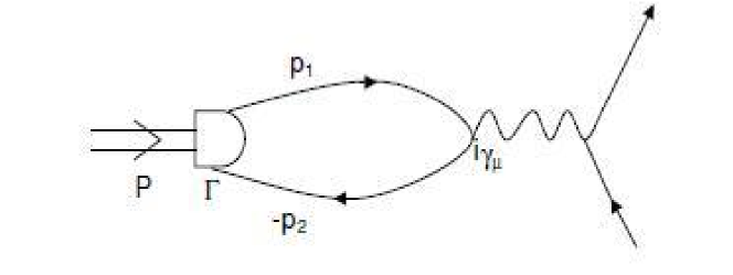
Figure 1: Quark loop diagram for $V\rightarrow\gamma^{*}\rightarrow e^{+}+e^{-}$ showing the coupling of electromagnetic current to the quark loop.

The coupling of a vector meson of momentum $P$ and polarization $\varepsilon_{\mu}$ to the photon is expressed via dimensionless coupling constant $g_{V}$ which can be described by the matrix element,

$$\ \frac{M^{2}}{g_{V}}\varepsilon_{\mu}(P)=\langle 0|\overline{Q}\widehat{\Theta}\gamma_{\mu}Q|V(P)\rangle$$ (21)

(where $Q$ is the flavour multiplet of quark field and $\widehat{\Theta}$ is the quark electromagnetic charge operator) which can in turn be expressed as a loop integral,

$$\ \frac{M^{2}}{g_{V}}\varepsilon_{\mu}(P)=\sqrt{3}e_{Q}\int d^{4}qTr[\Psi_{V}(P,q)i\gamma_{\mu}].$$ (22)

Here $e_{Q}$ arises from the flavour configuration of individual vector mesons and has values: $e_{Q}=1/\sqrt{2},1/3,1/\sqrt{18},2/3$ and $1/3$ for $\rho,\phi,\omega,\psi$ and $Y$ respectively, and the polarization vector $\varepsilon_{\mu}$ of V-meson satisfies, $\varepsilon\cdot P=0$. Defining leptonic decay constant,$f_{V}$ as, $f_{V}=M/(e_{Q}g_{V})$ bhatnagar06 , we can express

$$\ f_{V}\varepsilon_{\mu}(P)=\frac{\sqrt{3}}{M}\int d^{4}qTr\left[\Psi_{V}(P,q)i\gamma_{\mu}\right]$$ (23)

Plugging $\Psi_{V}(P,q)$, which involves the structure of hadron-quark vertex function in Eq. (2.8) flanked by the Dirac propagators of the two quarks as in Eq. (2.3), into the above equation, evaluating trace over the gamma matrices and noting that only the components of terms on the right hand side in the direction of $\varepsilon_{\mu}$ will contribute to the integral, we multiply both sides of the above integral by $P_{\mu}/M^{2}$, we can then express the leptonic decay constant $f_{V}$ as,

$$\ f_{V}=f_{V}^{0}+f_{V}^{1}+f_{V}^{2}+f_{V}^{3}+f_{V}^{4}+f_{V}^{5}$$ (24)

where $f_{V}^{0},f_{V}^{1},...,f_{V}^{5}$ are contributions to $f_{V}$ from the six Dirac structures associated with $A_{0},A_{1},...,A_{5}$ in the expression for hadron-quark vertex function $\Gamma(\widehat{q})$ and are expressed analytically in terms of $d\sigma$ integrations over the poles $\Delta_{1,2}$ of the quark propagators as:

$$\ f_{V}^{0} = \sqrt{3}N_{V}\frac{A_{0}}{M}\int d^{3}\widehat{q}D(\widehat{q})\phi(\widehat{q})\int\frac{Md\sigma}{2\pi i\Delta_{1}\Delta_{2}}4\left[\left(\frac{M^{2}}{6}+\frac{2}{3}m^{2}\right)+\frac{\Delta_{1}+\Delta_{2}}{6}\right]$$

$$\ f_{V}^{1} = \sqrt{3}N_{V}\frac{A_{1}}{M}\int d^{3}\widehat{q}D(\widehat{q})\phi(\widehat{q})\int\frac{Md\sigma}{2\pi i\Delta_{1}\Delta_{2}}(-4mM)$$

$$\ f_{V}^{2} = \sqrt{3}N_{V}\frac{A_{2}}{M}\int d^{3}\widehat{q}D(\widehat{q})\phi(\widehat{q})\int\frac{Md\sigma}{2\pi i\Delta_{1}\Delta_{2}}\left[-\frac{4}{3}m(\Delta_{1}-\Delta_{2})\right]$$

$$\ f_{V}^{3} = \sqrt{3}N_{V}\frac{A_{3}}{M}\int d^{3}\widehat{q}D(\widehat{q})\phi(\widehat{q})\int\frac{Md\sigma}{2\pi i\Delta_{1}\Delta_{2}}\left[-\frac{8}{3}(\Delta_{1}+\Delta_{2})+\left(\frac{16}{3}m^{2}-\frac{4}{3}M^{2}\right)\right]$$

$$\ f_{V}^{4} = \sqrt{3}N_{V}\frac{A_{4}}{M}\int d^{3}\widehat{q}D(\widehat{q)}\phi(\widehat{q})\int\frac{Md\sigma}{2\pi i\Delta_{1}\Delta_{2}}\left[-\frac{2m}{3M}(\Delta_{1}+\Delta_{2})+\left(\frac{4m^{3}}{3M}-\frac{1}{3}mM\right)\right]$$

$$\ f_{V}^{5} = \sqrt{3}N_{V}\frac{A_{5}}{M}\int d^{3}\widehat{q}D(\widehat{q)}\phi(\widehat{q})\int\frac{Md\sigma}{2\pi i\Delta_{1}\Delta_{2}}\left[\left(\frac{4}{3}m^{2}-\frac{2}{3}M^{2}\right)(\Delta_{1}-\Delta_{2})\right].$$ (25)

In deriving the above expressions, we have made use of the following relation showing the normalization over the polarization vector, $\varepsilon(P)$ for $V$- meson of 4-momentum, $P$ as,

$$\ \varepsilon_{\mu}\varepsilon_{\nu}=\frac{1}{3}\left(\delta_{\mu\nu}+\frac{P_{\mu}P_{\nu}}{M^{2}}\right),$$ (26)

We made use of the above relation to express the quantities involving dot products of $\varepsilon$ with various momenta like, $(p_{1}\cdot\varepsilon)(p_{2}\cdot\varepsilon)$, $(p_{1}\cdot\varepsilon)(q\cdot\varepsilon)$ and $(p_{2}\cdot\varepsilon)(q\cdot\varepsilon)$ in terms of dot products of momenta as,

$$\ (p_{1}\cdot\varepsilon)(p_{2}\cdot\varepsilon)=\frac{1}{3}p_{1}\cdot p_{2}-\frac{(p_{1}\cdot P)(p_{2}\cdot P)}{3M^{2}}$$

$$\ (p_{1}\cdot\varepsilon)(q\cdot\varepsilon)=\frac{1}{6}(p_{1}^{2}-p_{1}\cdot p_{2})-\frac{(p_{1}\cdot P)(p_{1}\cdot P-p_{2}\cdot P)}{6M^{2}}$$

$$\ (p_{2}\cdot\varepsilon)(q\cdot\varepsilon)=\frac{1}{6}(p_{1}\cdot p_{2}-p_{2}^{2})-\frac{(p_{2}\cdot P)(p_{1}\cdot P-p_{2}\cdot P)}{6M^{2}}$$ (27)

These dot products of momenta were in turn expressible in terms of the inverse propagators, $\Delta_{1,2}$ as:

$$p_{1}\cdot P = \frac{1}{2}(\Delta_{1}-\Delta_{2}-M^{2})$$

$$p_{2}\cdot P = \frac{1}{2}(-\Delta_{1}+\Delta_{2}-M^{2})$$

$$p_{1}\cdot p_{2} = m^{2}-\frac{1}{2}(\Delta_{1}+\Delta_{2}+M^{2})$$

$$p_{1,2}^{2} = \Delta_{1,2}-m^{2}$$

$$p_{1}\cdot q = \frac{3}{4}\Delta_{1}+\frac{1}{4}(\Delta_{2}+M^{2})-m^{2}$$

$$p_{2}\cdot q = -\frac{3}{4}\Delta_{2}-\frac{1}{4}(\Delta_{1}+M^{2})+m^{2}$$

$$P\cdot q = \frac{1}{2}(\Delta_{1}-\Delta_{2})$$ (28)

Thus all expressions for $f_{V}^{i}$ above were expressible in terms of $\Delta_{1,2}$. Then carrying out integrations over the off-shell variable, $d\sigma$ by the method of contour integrations by noting the pole positions in the complex $\sigma-$ plane:

$$\Delta_{1} = 0\Rightarrow\sigma_{1}^{\pm}=\pm\frac{\omega_{1}}{M}-\widehat{m}_{1}\mp i\epsilon,$$

$$\Delta_{2} = 0\Rightarrow\sigma_{2}^{\mp}=\mp\frac{\omega_{2}}{M}-\widehat{m}_{2}\pm i\epsilon,$$

$$\omega_{1}^{2} = \omega_{2}^{2}=m^{2}+\widehat{q}^{2}$$

$$\widehat{m}_{1} = \widehat{m}_{2}=\frac{1}{2}$$ (29)

we get, the following integrals:

$$\int\frac{Md\sigma}{\Delta_{1}\Delta_{2}}(\Delta_{1}+\Delta_{2}) = D_{0}(\widehat{q});$$

$$\int\frac{Md\sigma}{\Delta_{1}\Delta_{2}} = \frac{1}{D(\widehat{q})},$$ (30)

where,

$$D(\widehat{q}) = \omega D_{0}(\widehat{q}),$$

$$D_{0}(\widehat{q}) = 4\omega^{2}-M^{2}.$$ (31)

Thus we can express the various components $f_{V}^{i}$ $(i=0,...,5)$ of $f_{V}$ in Eq. (3.5) as,

$$\ f_{V}^{0}=\sqrt{3}N_{V}\frac{A_{0}}{M}\int d^{3}\widehat{q}\phi(\widehat{q})4\left[\frac{M^{2}}{6}+\frac{2}{3}m^{2}+\frac{D_{0}(\widehat{q})}{6}\right]$$

$$\ f_{V}^{1}=\sqrt{3}N_{V}\frac{A_{1}}{M}\int d^{3}\widehat{q}\phi(\widehat{q})(-4mM)$$

$$\ f_{V}^{2}=0$$

$$\ f_{V}^{3}=\sqrt{3}N_{V}\frac{A_{3}}{M}\int d^{3}\widehat{q}\phi(\widehat{q})\left[-\frac{8}{3}D_{0}(\widehat{q})+\frac{16}{3}m^{2}-\frac{4}{3}M^{2}\right]$$

$$\ f_{V}^{4}=\sqrt{3}N_{V}\frac{A_{4}}{M}\int d^{3}\widehat{q}\phi(\widehat{q})\left[-\frac{2m}{3M}D_{0}(\widehat{q})+\frac{4m^{3}}{3M}-\frac{1}{3}mM\right]$$

$$\ f_{V}^{5}=0$$ (32)

Note that the components, $f_{V}^{2}$ and $f_{V}^{5}$ are $0$ on account of equal mass kinematics.

Note that each of the $f_{V}^{i}$ involves the BS normalizer $N_{V}$. This is evaluated using the current conservation condition:bhatnagar06 ; bhatnagar11 ; elias11 ,

$$2iP_{\mu}=(2\pi)^{4}\int d^{4}q\mbox{Tr}\left\{\overline{\Psi}(P,q)\left[\frac{\partial}{\partial P_{\mu}}S_{F}^{-1}(p_{1})\right]\Psi(P,q)S_{F}^{-1}(-p_{2})\right\}+(1\rightleftharpoons 2)$$ (33)

Putting BS wave function $\Psi(P,q)$ for a vector meson in Eqs. (2.3) and (2.8) in the above equation, carrying out derivatives of inverse quark propagators of constituent quarks with respect to total hadron momentum $P_{\mu}$, evaluating trace over products of gamma matrices, following usual steps, and multiplying both sides of the equation by $P_{\mu}/(-M^{2})$ to extract out the normalizer $N_{V}$ from the above equation, we then express the above equation in terms of the integration variables $\widehat{q}$ and $\sigma$. Noting that the 4D volume element $d^{4}q=d^{3}\widehat{q}Md\sigma$, we then perform the contour integration in the complex $\sigma$- plane by making use of the corresponding pole positions. For details of these mathematical steps involved in the calculations of BS normalizers for vector and pseudoscalar mesons see bhatnagar06 ; bhatnagar11 , where in the present calculation, we take both, the leading order (LO) as well as the next-to-leading order (NLO) Dirac structures for vector mesons in their respective 4D BS wave functions $\Psi(P,q)$. Then integration over the variable $\widehat{q}$ is finally performed to extract out the numerical results for $N_{V}$ for different vector mesons. The calculation of $N_{V}$ is quite complex due to the $6$ Dirac structures involved in the calculation. The structure of the normalizer is of the form,

$$N_{V}^{-2}=i(2\pi)^{2}\int d^{3}\widehat{q}D^{2}(\widehat{q})\phi^{2}(\widehat{q})\displaystyle\sum\limits_{ij}A_{i}A_{j}I_{ij}(m,M,\widehat{q},S).$$ (34)

Here, $A=(A_{0},A_{1},A_{2},A_{3},A_{4},A_{5})$ are functions of parameters $A_{i}$, $S=(R,D_{1},D_{2},D_{11},$ $D_{12},D_{22})$, where the $S_{i}$ are the results of integrations over off-shell parameter $\sigma$ whose results are given in Eq. (36). The $I_{ij}(m,M,\widehat{q},R)$ are involved functions of $m,M,\widehat{q}$ and $R$. Explicit expressions are listed below in Eq. (III.1):

$$I_{00} = \frac{1}{3}\left[\frac{1}{M^{2}}\left(1-12\frac{m^{2}}{M^{2}}\right)D_{11}+\frac{3}{M^{2}}\left(-1+\frac{m^{2}}{M^{2}}\right)D_{12}+\frac{1}{M^{2}}(7m^{4}-3m^{2}M^{2})R\right.$$

$$\left.+\frac{1}{M^{2}}\left(M^{2}+\frac{13m^{4}}{M^{2}}-5m^{2}\right)D_{1}-\frac{13m^{4}D_{2}}{M^{4}}+\frac{9m^{2}D_{22}}{M^{4}}\right]$$

$$I_{11} = \frac{2}{3}\left[-\frac{4D_{11}}{M^{2}}+\frac{3D_{12}}{M^{2}}-\frac{4D_{22}}{M^{2}}-\frac{8M^{2}D_{1}}{M^{2}}+\frac{(8m^{2}+M^{2})D_{2}}{M^{2}}+2(4m^{2}+M^{2})R\right]$$

$$I_{22} = \frac{2}{3}\left[\frac{D_{11}}{M^{2}}+\frac{3D_{12}}{M^{2}}-\frac{4D_{22}}{M^{2}}-\frac{8m^{2}D_{1}}{M^{2}}+\frac{(8m^{2}+M^{2})D_{2}}{M^{2}}+2(4m^{2}+M^{2})R\right]$$

$$I_{33} = \frac{1}{3}\left[\frac{D_{11}}{M^{2}}\left(\frac{-6m^{4}}{M^{4}}+\frac{9m^{2}}{M^{2}}-\frac{22m^{3}}{M^{3}}-\frac{55m^{2}}{2M^{2}}+13\right)\right.$$

$$+\frac{D_{12}}{M^{2}}\left(\frac{18m^{4}}{M^{4}}-\frac{7m^{2}}{M^{2}}+\frac{70m^{2}}{M^{2}}+\frac{12m^{3}}{M^{3}}-4\right)$$

$$+\frac{D_{22}}{M^{2}}\left(\frac{9m^{4}}{M^{4}}-\frac{67m^{2}}{M^{2}}+\frac{10m^{3}}{M^{3}}+35-\frac{9m^{2}}{M^{2}}\right)$$

$$+\frac{D_{1}}{M^{2}}\left(\frac{29}{2}M^{2}-13m^{2}+\frac{12m^{4}}{M^{2}}-\frac{3m^{3}}{M}-\frac{48m^{4}}{M^{2}}+\frac{16m^{6}}{M^{4}}-\frac{36m^{5}}{M^{3}}\right)$$

$$+\frac{D_{2}}{M^{2}}\left(22M^{2}-7m^{2}-\frac{12m^{4}}{M^{2}}+\frac{3m^{3}}{M}+\frac{48m^{4}}{M^{2}}-\frac{16m^{6}}{M^{4}}+\frac{4m^{5}}{M^{3}}\right)$$

$$\left.+\frac{R}{M^{2}}\left(-m^{2}M^{2}-14m^{3}M+76m^{4}+16mM^{3}+6M^{4}+\frac{5}{2}m^{4}\right)\right]$$

$$I_{44} = \frac{1}{3}\left[\frac{D_{11}}{M^{2}}\left(\frac{4m^{2}}{M^{2}}+1\right)+\frac{7D_{12}}{2M^{2}}+\frac{D_{22}}{M^{2}}\left(\frac{1}{6}-\frac{4m^{2}}{M^{2}}\right)\right.$$

$$+\left(2-\frac{6m^{4}}{M^{4}}-\frac{m^{5}}{M^{5}}-\frac{6m^{2}}{M^{2}}-\frac{m^{3}}{M^{3}}\right)D_{1}+\left(\frac{1}{6}+\frac{m^{5}}{M^{5}}+\frac{6m^{4}}{M^{4}}-\frac{8m^{2}}{M^{2}}\right)D_{2}$$

$$\left.+\left(-4m^{2}+\frac{8m^{4}}{M^{2}}+\frac{m^{5}}{M^{3}}+\frac{M^{2}}{3}\right)R\right]$$

$$I_{55} = \frac{1}{3}\left[-\frac{3}{2M^{2}}\left(\frac{m^{4}}{3M^{4}}+\frac{11m^{2}}{3M^{2}}+\frac{3}{2}\right)D_{12}+\frac{D_{1}}{M^{2}}\left(-M^{2}+\frac{3m^{4}}{2M^{2}}+\frac{7m^{5}}{2M^{3}}+\frac{17m^{2}}{4}\right)\right.$$

$$\left.+\frac{D_{2}}{M^{2}}\left(-\frac{M^{2}}{4}-\frac{3m^{5}}{2M^{3}}-\frac{7m^{4}}{2M^{2}}+\frac{15m^{2}}{4}\right)+\frac{R}{M^{2}}\left(-\frac{3M^{4}}{2}+\frac{9m^{2}M^{2}}{4}+\frac{7m^{4}}{2}\right)R\right]$$

$$I_{01} = \left[-\frac{4mD_{11}}{M^{3}}-\frac{8mD_{22}}{M^{3}}+\frac{4mD_{12}}{M^{3}}-\frac{4D_{1}}{3M}\left(\frac{4m^{3}}{M^{2}}+m\right)\right.$$

$$\left.+\frac{4D_{2}}{M}\left(\frac{4m^{3}}{3M^{2}}-m\right)+\left(\frac{16m^{3}}{3M}-\frac{4mM}{3}R\right)\right]$$

$$I_{02} = \left[\frac{8m}{M}(D_{1}-D_{2})-8mMR\right];$$

$$I_{03} = \left[-\frac{2m}{M^{3}}D_{11}+\frac{4m}{3M^{3}}D_{12}+\frac{2m}{M^{3}}D_{22}+\frac{8D_{1}}{3M}(\frac{m^{3}}{M^{2}}-m)+\frac{3m^{3}}{3M^{3}}D_{2}\right.$$

$$\left.+(\frac{8m^{3}}{3M}-\frac{2mM}{3})R\right]$$

$$I_{04} = \left[-\frac{7m^{2}D_{11}}{3M^{4}}+\frac{D_{22}}{3M^{2}}\left(-\frac{2m^{4}}{M^{4}}-\frac{7m^{2}}{M^{2}}+8\right)+\frac{D_{12}}{3M^{2}}\left(\frac{2m^{2}}{M^{2}}-8\right)\right.$$

$$\left.+\frac{D_{1}}{M^{2}}\left(-M^{2}-\frac{2m^{4}}{3M^{2}}+\frac{8m^{2}}{3}\right)+\frac{D_{2}}{M^{2}}\left(\frac{4M^{2}}{3}+\frac{2m^{4}}{3M^{2}}-\frac{8m^{2}}{3})+\frac{R}{M^{2}}(-m^{2}M^{2}-2m^{4}\right)\right]$$

$$I_{05} = \left[\frac{D_{11}}{M^{2}}\left(\frac{6m^{2}}{M^{2}}-\frac{34}{3}\right)+\frac{D_{22}}{3M^{2}}\left(\frac{26m^{2}}{M^{2}}-14\right)-\frac{D_{12}}{3M^{2}}\left(\frac{44m^{2}}{M^{2}}+20\right)\right.$$

$$+\frac{D_{1}}{M^{2}}\left(-6M^{2}+\frac{8m^{4}}{3M^{2}}-12m^{2}\right)D_{1}+\frac{D_{2}}{M^{2}}\left(-\frac{22M^{2}}{3}-\frac{8m^{4}}{M^{2}}+\frac{44m^{2}}{3}\right)$$

$$+\frac{R}{M^{2}}\left(14m^{2}M^{2}-\frac{8m^{4}}{3}-\frac{10M^{4}}{3}\right)\}$$

$$I_{12} = \left[\frac{D_{11}}{M^{2}}\left(\frac{m^{2}}{M^{2}}+\frac{2}{3}\right)+\frac{D_{22}}{M^{2}}\left(\frac{m^{2}}{M^{2}}-4\right)+\frac{D_{12}}{M^{2}}\left(-\frac{2m^{2}}{M^{2}}+\frac{10}{3}\right)\right.$$

$$\left.+\frac{D_{1}}{M^{2}}\left(\frac{8M^{2}}{3}-\frac{2m^{2}}{3}\right)+\frac{D_{2}}{M^{2}}\left(-2M^{2}+\frac{2m^{2}}{3}\right)+\frac{5m^{2}R}{3}\right]$$

$$I_{13} = \left[\frac{D_{11}}{3M^{3}}\left(-\frac{4m^{3}}{M^{2}}-34m\right)+\frac{D_{22}}{3M^{3}}\left(-\frac{4m^{3}}{M^{2}}-26m\right)+\left(\frac{8m^{2}}{M^{4}}+\frac{20}{M^{2}}\right)D_{12}\right.$$

$$+\frac{D_{22}}{M^{3}}\left(-\frac{16m^{5}}{3M^{4}}+\frac{8m^{3}}{3M^{2}}+28m\right)+\frac{D_{2}}{M}\left(\frac{16m^{5}}{3M^{4}}-\frac{8m^{3}}{3M^{2}}-\frac{46m}{3}\right)$$

$$\left.+\left(-\frac{28m^{4}}{3M^{2}}-\frac{8m^{3}}{3M}-2mM\right)R\right]$$

$$I_{14} = \left[\frac{D_{11}}{M^{2}}\left(-\frac{m^{4}}{M^{4}}+\frac{4}{3}\right)+\frac{D_{22}}{M^{2}}\left(-\frac{m^{2}}{M^{2}}+2\right)+\frac{D_{12}}{M^{2}}\left(\frac{2m^{2}}{M^{2}}-\frac{10}{3}\right)\right.$$

$$\left.+\frac{D_{1}}{M^{2}}\frac{13m^{2}}{3}-\frac{D_{2}}{M^{2}}\frac{5m^{2}}{3}+\left(-\frac{8m^{2}}{3}+\frac{2M^{2}}{3}\right)R\right]$$

$$I_{15} = \left[\frac{5m}{3M^{3}}D_{11}-\frac{m}{3M^{3}}D_{22}-\frac{4m}{3M^{3}}D_{12}+\frac{D_{2}}{M}\left(-\frac{2m^{3}}{M^{2}}+\frac{2m}{3}\right)D_{2}+\left(-\frac{2m^{3}}{M}+mM\right)R\right]$$

$$I_{23} = \left[\left(\frac{7m^{3}}{3M^{5}}+\frac{3m^{2}}{4M^{4}}+\frac{5m}{12M^{3}}\right)D_{11}+\left(\frac{7m^{3}}{3M^{5}}-\frac{3m^{2}}{6M^{4}}\right)D_{22}\right.$$

$$+\left(-\frac{14m^{3}}{3M^{5}}+\frac{m}{3M^{3}}-\frac{3m^{2}}{4M^{4}}\right)D_{12}$$

$$+\left(-\frac{7m^{3}}{6M^{3}}+\frac{m}{6M}-\frac{3m^{4}}{8M^{4}}+\frac{3m^{2}}{8M^{2}}\right)D_{1}+D_{2}\left(\frac{7m^{3}}{6M^{3}}-\frac{m}{M}+\frac{3m^{4}}{8M^{4}}\right)$$

$$\left.+\left(\frac{5m^{3}}{6M}-\frac{mM}{4}+\frac{3m^{4}}{16M^{2}}\right)R\right];$$

$$I_{24} = \left[\frac{13m^{3}}{M}R+\frac{D_{11}}{M^{3}}\left(-\frac{3m^{3}}{2M^{2}}+\frac{7m}{3}\right)-\frac{D_{22}}{M^{3}}\left(\frac{m^{3}}{3M^{2}}+6m\right)+\frac{D_{12}}{M^{3}}\left(\frac{3m^{3}}{M^{2}}+\frac{11m}{3}\right)\right.$$

$$\left.+\frac{D_{1}}{3M}\left(-\frac{25m^{3}}{M^{2}}-5m\right)+\frac{D_{2}}{3M}\left(\frac{25m^{3}}{M^{2}}-19m\right)\right]$$

$$I_{25} = \left[\frac{D_{11}}{M^{2}}\left(-\frac{3m^{2}}{2M^{2}}+\frac{4m^{4}}{M^{4}}+1\right)+\frac{D_{22}}{M^{2}}\left(-\frac{7m^{2}}{2M^{2}}-\frac{4m^{4}}{3M^{4}}+\frac{10}{3}\right)\right.$$

$$+\frac{D_{1}}{M^{2}}\left(\frac{7M^{2}}{6}+\frac{m^{4}}{M^{2}}-10\frac{4m^{2}}{3}-\frac{8m^{6}}{3M^{4}}\right)+\frac{D_{2}}{M^{2}}\left(\frac{8M^{2}}{3}-\frac{m^{4}}{3M^{2}}+\frac{8m^{6}}{3M^{4}}-8m^{2}\right)$$

$$\left.+\frac{D_{1}D_{2}}{M^{2}}\left(\frac{5m^{2}}{M^{2}}-\frac{8m^{4}}{3M^{4}}+2\right)+\left(-\frac{23m^{2}}{6}+\frac{19m^{4}}{3M^{2}}+\frac{8m^{6}}{3M^{4}}+\frac{2M^{2}}{3}\right)R\right]$$

$$I_{34} = \left[-\frac{m^{3}}{M^{5}}\left(D_{11}+D_{22}\right)+\frac{4m^{3}}{M^{5}}D_{12}\right]$$

$$I_{35} = \left[\frac{D_{11}}{M^{2}}\left(\frac{m^{4}}{M^{4}}+\frac{28m^{2}}{M^{2}}-\frac{16m^{4}}{M^{4}}-\frac{14}{3}\right)+\frac{D_{22}}{M^{2}}\left(\frac{m^{2}}{M^{2}}-\frac{8m^{4}}{3M^{4}}+\frac{16m^{3}}{M^{3}}-\frac{2}{3}\right)\right.$$

$$+\frac{D_{1}}{M^{2}}\left(\frac{2M^{2}}{3}-\frac{10m^{3}}{M}-\frac{2m^{4}}{3M^{2}}+\frac{16m^{6}}{3M^{4}}+\frac{22m^{2}}{3}\right)+\frac{D_{2}}{M^{2}}\left(2M^{2}-\frac{12m^{2}}{3}+\frac{26m^{4}}{3M^{2}}-\frac{2m^{4}}{3M^{2}}-\frac{16m^{6}}{3M^{4}}\right)$$

$$\left.+\frac{D_{12}}{M^{2}}\left(-\frac{2m^{4}}{3M^{4}}+\frac{50m^{2}}{3M^{2}}+\frac{4}{3}\right)+\frac{R}{M^{2}}\left(-2m^{4}-\frac{8M^{4}}{3}-\frac{14m^{6}}{3M^{2}}-\frac{10m^{2}M^{2}}{3}\right)\right]$$

$$I_{45} = \left[\frac{D_{11}}{M^{3}}\left(-\frac{8m^{3}}{M^{2}}-\frac{8m}{3}\right)+\frac{D_{22}}{M^{3}}\left(-\frac{8m^{3}}{M^{2}}+\frac{16m}{3}\right)+\frac{D_{12}}{M^{3}}\left(\frac{16m^{3}}{M^{2}}-\frac{8m}{3}\right)\right.$$

$$\left.\frac{D_{1}}{M^{2}}\left(\frac{8m^{3}}{M^{2}}-\frac{4m}{3}\right)+\frac{D_{2}}{M}\left(-\frac{8m^{3}}{M^{2}}+\frac{4m}{3}\right)\right]$$

       (35)

Here $R,D_{1},D_{2},D_{11},D_{12},D_{22}$ are the analytic results of contour integrations over the off-shell parameter $d\sigma$ in the complex $\sigma$-plane. The results of these integrals are given as:

$$D_{1} = \int\frac{Md\sigma}{\Delta_{1}^{2}\Delta_{2}}\Delta_{1}=2\pi i\;\frac{1}{D(\widehat{q})}$$

$$D_{2} = \int\frac{Md\sigma}{\Delta_{1}^{2}\Delta_{2}}\Delta_{2}=2\pi i\;\frac{2}{(2\omega)^{3}}$$

$$D_{12} = \int\frac{Md\sigma}{\Delta_{1}^{2}\Delta_{2}}\Delta_{1}\Delta_{2}=2\pi i\;\frac{1}{2\omega}$$

$$D_{11} = \int\frac{Md\sigma}{\Delta_{1}^{2}\Delta_{2}}\Delta_{1}^{2}=2\pi i\;\frac{1}{2\omega}$$

$$D_{22} = \int\frac{Md\sigma}{\Delta_{1}^{2}\Delta_{2}}\Delta_{2}^{2}=2\pi i\;\frac{\displaystyle\omega^{2}-\frac{M^{2}}{2}}{\omega^{3}}$$

$$R = \int\frac{Md\sigma}{\Delta_{1}^{2}\Delta_{2}}=2\pi i\;\frac{M^{2}-12\omega^{2}}{4\omega^{3}(M^{2}-4\omega^{2})^{2}}$$ (36)

Final result for the BS normalizer has the form,

$$N_{V}^{-2} = \frac{\pi^{5/2}}{72M^{7}\beta^{3}}e^{m^{2}/(2\beta^{2})}\left\{[G_{13}(m,M,A)+G_{11}(m,M,A)\beta^{2}+G_{9}(m,M,A)\beta^{4}]K_{0}\left(\frac{m^{2}}{2\beta^{2}}\right)\right.$$ (37)

$$+[G_{13}(m,M,A)+G_{11}(m,M,A)\beta^{2}+G_{9}(m,M,A)\beta^{4}+G_{7}(m,M,A)\beta^{6}]K_{1}\left(\frac{m^{2}}{2\beta^{2}}\right)$$

$$+\left[H_{5}(m,M)\beta^{6}U\left(\frac{1}{2},-3,\frac{m^{2}}{\beta^{2}}\right)\right.$$

$$+H_{7}(m,M)\beta^{4}U\left(\frac{1}{2},-2,\frac{m^{2}}{\beta^{2}}\right)$$

$$\left.\left.+H_{11}(m,M)U\left(\frac{1}{2},0,\frac{m^{2}}{\beta^{2}}\right)\right]\beta^{2}A_{3}A_{5}\right\}.$$

Here, $K_{n}(x)$ is the second class modified Bessel function, $U(a,b,x)$ is the confluent hypergeometric function, $G_{n}$ and $H_{n}$ are polynomials of $n$-th degree in $m$ and $M$, and the $G_{n}$ are quadratic functions of the $A_{i}$ coefficients.

In these expressions, $\phi(\hat{q})$ is a decaying function of $\hat{q}^{2}$. Thus despite the fact that the integrands contain growing factors like $\hat{q}^{2}$, the overall integrals converge, and can be analytically integrated. Then, the $f_{V}^{i}$ $(i=0,...,5)$ can be expressed in the following analytic form,

$$f_{V}^{0} = \frac{A_{0}}{M}N_{V}16\sqrt{\frac{2}{3}}\pi^{3/4}\beta^{3/2}(2m^{2}+3\beta^{2})$$

$$f_{V}^{1} = -A_{1}N_{V}8\sqrt{6}\pi^{3/4}\beta^{3/2}m$$

$$f_{V}^{2} = 0$$

$$f_{V}^{3} = \frac{A_{3}}{M^{2}}N_{V}\frac{2\pi^{1/4}}{\sqrt{3}}\sqrt{\beta}\left\{3M\sqrt{2\pi}\beta(-4m^{2}+M^{2}-28\beta^{2})\phantom{\frac{2}{4}}\right.$$

$$\left.+2e^{m^{2}/(4\beta^{2})}m^{2}\left[2m^{2}K_{0}\left(\frac{m^{2}}{4\beta^{2}}\right)\ +(2m^{2}-M^{2}+16\beta^{2})K_{1}\left(\frac{m^{2}}{4\beta^{2}}\right)\right]\right\}$$

$$f_{V}^{4} = -\frac{A_{4}}{M^{3}}N_{V}\frac{4\pi^{1/4}}{\sqrt{3}}\sqrt{\beta}\left\{m^{2}M^{2}e^{m^{2}/(4\beta^{2})}K_{1}\left(\frac{m^{2}}{4\beta^{2}}\right)+2\sqrt{\pi}\beta^{3}\left[3\sqrt{2}M-8\beta U\left(-\frac{3}{2},-2,\frac{m^{2}}{2\beta^{2}}\right)\right]\right\}$$

$$f_{V}^{5} = 0$$ (38)

with $N_{V}$ given in the previous equation.

IV Results

IV.1 Numerical Calculation

Eq. (3.18) which expresses decay constants $f_{V}$ of vector mesons in terms of the parameters $A\equiv($$A_{0}$, $A_{1}$, $A_{2}$, $A_{3}$, $A_{4}$, $A_{5})$ is a non linear function of the $A_{i}$’s. Then numerical methods must be applied to solve the problem of determining the best values of the $A_{i}$’s.

We used a simple ‘Mathematica’ procedure for searching for accurate values of the $A_{i}$ ($i=0,...5$). We defined the following auxiliary function $W(A)$, which is positive definite, as,

$$W(A)=\sum\limits_{V}\left[f_{V}(A)-f_{V}^{EXP}\right]^{2}.$$ (39)

The summation in the above equation runs over the five ground state vector mesons $\rho$, $\omega$, $\phi$, $\psi$ and $Y$ studied in this work. $f_{V}^{EXP}$ are the central values of experimental data on decay constants used (indicated in Table 2) which are calculable from the data on the partial widths, $\Gamma(e^{+}+e^{-})$ for the five studied mesons in  beringen12 . Their results are the following: $\rho$(770): 7.04$\pm$0.06 keV, $\omega$(782): 0.60$\pm$0.02 keV, $\phi$(1020): 1.27$\pm$0.04 keV, $\psi$(1S): 5.5$\pm$0.1 keV, $Y$(1S): 1.34$\pm$0.02 keV. They are related to our decay constants $f_{V}$ by formula,

$$\Gamma=\frac{4\pi\alpha^{2}e_{Q}^{2}|f_{V}|^{2}}{3M}.$$ (40)

Here, $M$ is the meson mass, $\alpha$ is the QED coupling constant (i.e. the fine structure constant), $e_{Q}$ plays the role of effective electric charge of the meson and has values as listed after Eq.(3.2)for different vector mesons.

From formula (40) were obtained the data cited in Table 1. We see that the error bars of experimental data on decay widths given by PDG tables for the $\rho$, $\omega$, $\phi$, $\psi$ and $Y$ mesons represent, 0.8%, 3.3%, 3.1%, 1.8%, 1.5%, respectively. We can say that average error bars are 2.1% or 0.05 keV. The average error in decay constants derived from experimental data of the five mesons studied is 1%. As a general rule, while we are averaging data coming from different measurements, we should give larger weight to more precise data and lesser weight to less precise data. For instance, $\rho$’s experimental error bar of $f_{V}$ is 0.4%, while for $\omega$ meson error bar of $f_{V}$ is 1.6%; i.e. $\rho$ has a higher precision than $\omega$ meson. However, by using the $W(A)$ function, we have fit the data for all mesons from $\rho$ to $Y$ at the same level. This means that we can not expect a fitting with an average error significantly less than $\sim 1.6$%.

From the numerical point of view, the problem reduces to finding values of $A_{i}$’s such that $W(A)$ has a minimum, and that at such a minimum it takes the value zero. We used the Mathematica package which has some useful functions for minimizing. It is clear that the 6-dimensional hypersurface $W(A)$ has many minima, but the only acceptable minima are those minima for which $W(A)$ is very close to zero. The experimental values of the $f_{V}$’s are 0.220, 0.195, 0.228, 0.410 and 0.708 GeV. Then, we adopt as criterium of “sufficient closeness” to zero the value of $W(A)$ which is less than $0.02^{2}=0.0004$ GeV².

Besides, it is important to ensure a degree of robustness of the solution. It means, that if we change each of the experimental values $f_{V}^{EXP}$ according to their error bars, then the values of the $A_{i}$ which minimize $W(A)$ remain near the corresponding values which minimize at the central values $f_{V}^{EXP}$. This is the main criterion of stability which must be satisfied for the model to be physically acceptable. In other words, when point $(A)$ is within a box determined by the averages and the error bars of the $A_{i}$, the function $W(A)$ has a minimum very near to zero for $f_{V}$ in a box determined by the experimental data of the $f_{V}$ and their error bars.

An additional check is done by evaluating the percent average of the absolute values of the differences between the predicted $f_{V}$ values from the experimental value $f_{V}^{EXP}$.

Using this method, we found that the values of coefficients should respectively be: $A_{0}=1$, $A_{1}=0.006773$, $A_{2}=1.24011$, $A_{3}=-0.414747$, $A_{4}=0.013611$, $A_{5}=-1.84191$ to predict the decay constant values, $f_{\rho}=0.207440$ GeV, $f_{\omega}=0.206914$ GeV, $f_{\phi}=0.230219$ GeV, $f_{\psi}=0.415707$ GeV, and $f_{Y}=0.758994$ GeV. These decay constant values have an average error with respect to the experimental data of 4%.

The robustness of the model can be quantified in the following way. The set of $A_{i}$ which, when replaced in $f_{V}(A)$ give a value “near” the experimental value of the decay constant for each of the studied vector mesons. We found that point $(A)$ is located within certain “box” of sides $2\Delta A_{i}=0.008$. The center of the box is at the values given in the last paragraph. All those results were obtained by randomly choosing 22 sets of the $f_{V}$ within their experimental error bars and finding in each case the point $A$ where $W(A)$ has a minimum near to zero. Fig. 2 represents the $f_{V}$ amplitudes for all five studied mesons, sets of dots were obtained by varying the $A_{i}$ coefficients around their average values, procedure was done to show stability of results.

The normalization factors $N_{V}$ were found to be: $N_{\rho}=0.18707795$ GeV^-3, $N_{\omega}=0.18624605$ GeV^-3, $N_{\phi}=0.13413963$ GeV^-3, $N_{\psi}=0.03270152$ GeV^-3, and $N_{Y}=0.00495780$ GeV^-3. Values of $f_{V}$ along with the contributions from various covariants and experimental results are listed in Table 2. Comparison of our results with those of other models and data is presented in Table 3.

IV.2 The results

Formulas found in section II express decay constants $f_{V}$ of vector mesons in terms of the constant parameters $A_{0}$, $A_{1}$, $A_{2}$, $A_{3}$, $A_{4}$, $A_{5}$. Our model should be capable of predicting the values of those parameters if one uses the known experimental values of the decay constants for the $\rho$, $\omega$, $\phi$, $\psi$, $\psi^{\prime}$ and $Y$ mesons. Expression for $f_{V}$ in Eq. (3.12) and Eq. (3.18) is a linear function of the $A_{i}$’s (for i=0,1,2,3,4,5). However $f_{V}$ involves the BS normalizer $N_{V}$, which is evaluated by integrating with respect to $\hat{q}$, is a highly non-linear function of the $A_{i}$’s. Analytical expressions for the $A_{i}$’s as functions of quark masses and other parameters corresponding to each of the vector mesons can not be obtained. However, numerical methods give acceptable solutions of the problem.

Expression for normalizer (37) has the form,

$$\frac{1}{N_{V}^{2}}=\sum\limits_{i=0}^{5}\sum\limits_{j=i}^{5}I_{ij}A_{i}A_{j},$$ (41)

where matrix elements $I_{ij}$ were given in Eq. (III.1).

Contributions $f_{V}^{i}$ to the decay constants, given by Eq. (38), by definition are proportional to $A_{i}$,

$$f_{V}=\sum\limits_{i=0}^{5}f_{V}^{i}\equiv\sum\limits_{i=0}^{5}\frac{f_{V_{i}}}{N_{V}}A_{i}.$$ (42)

Our idea is that the $A_{i}$ can be obtained by fitting formulas to experimental results,

$$\frac{\sum\limits_{i=0}^{5}f_{V_{i}}A_{i}}{\sqrt{\sum\limits_{i=0}^{5}\sum\limits_{j=i}^{5}I_{ij}A_{i}A_{j}}}=f_{V}^{EXP}.$$ (43)

(see Eq. (34) and Eq. (III.1)). We must notice that 43 is a homogenous function of the $A_{i}$, fact that precludes finding solutions for the $A_{0},...A_{5}$ by using available data of the five considered mesons. However, a nonhomogenous system of equations can be constructed by putting $A_{0}=1$ and leaving as unknowns $A_{1},...A_{5}$. With this procedure it is sufficient to consider the five mesons $\rho$, $\omega$, $\phi$, $\psi$, and $Y$. System of five equations is obtained by introducing in Eq. (43) the appropriate parameters of the five mesons.

For the $f_{V}^{EXP}$ we used the results from PDG tables beringen12 . We see that the “error bars” on data for $f_{V}$ for $\rho,\omega,\phi,\psi$ and $Y$ mesons are 0.4%, 1.7%, 1.6%, 0.9% and 0.8% respectively, whose average is about 1.1%.

System of five equations has many solutions, several of them complex. Complex solutions appear in conjugate pairs. Available algorithms allow finding all solutions with very high precision. In this way the percent average of the absolute values of the difference between the calculated $f_{V}$ and the $f_{V}^{EXP.}$ experimentally found, is much lower than the error bars of experiments. However the values of the $A_{i}$ found were complex, which lead to complex $f_{V}$’s. We made different checks and selected the parameter set giving the results shown in Table 2 which predicts the experimental values of all the $f_{V}$’s with less precision. The $f_{V}$’s predicted for the considered mesons match approximately with the experimental values. Regarding meson $\psi^{\prime}$, our theoretical value is 0.1798 GeV, while value calculated from experiments is 0.2200 GeV, with error 18%.

Table 1: Some parameters of vector mesons. $M$ is meson mass, $m$ is mass of quark constituent, $\beta$ is the inverse range parameter appearing in BS wave function, $\Gamma^{EXP.}$ is the experimental value of width beringen12 and $f_{V}^{EXP.}$ is the decay constant deduced from $\Gamma^{EXP.}$ by using formula Eq. (40). $e_{Q}$ arises from the flavor configuration of individual vector mesons.

Meson	$m$ (GeV)	$M$ (GeV)	$e_{Q}$	$\beta$	$\Gamma^{EXP.}$ (keV)	$f_{V}^{EXP.}$ (GeV)
$\rho(770)$	0.265	0.7755$\pm$0.0003	$1/\sqrt{2}$	0.265294	7.04$\pm$0.06	0.2201$\pm 0.0009$
$\omega(782)$	0.265	0.7827$\pm$0.0001	$1/\sqrt{18}$	0.2661	0.60$\pm$0.02	0.195$\pm 0.003$
$\phi(1020)$	0.415	1.01946$\pm$0.00002	$1/3$	0.293347	1.27$\pm$0.04	0.228$\pm 0.003$
$J/\psi(1S)$	1.532	3.09692$\pm$0.00001	$2/3$	0.444214	5.5$\pm$0.1	0.410$\pm 0.003$
$Y(1S)$	4.9	9.4603$\pm$0.0003	$1/3$	0.721345	1.34$\pm$0.02	0.708$\pm 0.005$

Table 2: Decay constant $f_{V}^{TH.}$ values (in GeV) for $\rho$, $\omega$, $\phi$, $\psi$ and $Y$ mesons in BSE-CIA with the individual contributions $f_{V}^{0}$, $f_{V}^{1}$, $f_{V}^{2}$, $f_{V}^{3}$, $f_{V}^{4}$, $f_{V}^{5}$ from various Dirac covariants along with the contributions from LO and NLO covariants and also their % contributions for parameter set: $A_{0}=1$, $A_{1}=0.00677$, $A_{2}=1.24011$, $A_{3}=-0.41474$, $A_{4}=0.01361$, $A_{5}=-1.84191$ (with average error with respect to the experimental data of 4%)

	$f_{V}^{0}$	$f_{V}^{1}$	$f_{V}^{3}$	$f_{V}^{4}$	$f_{V}^{LO}$	$f_{V}^{NLO}$	$f_{V}^{LO}$(%)	$f_{V}^{NLO}$(%)	$\bm{f_{V}^{TH.}}$	$\bm{f_{V}^{EXP}}$
$\rho$	0.1156	-0.00068	0.09336	-0.00026	0.1149	0.0931	55%	45%	0.2080	0.2200
$\omega$	0.1155	-0.000689	0.093	-0.000258	0.1148	0.0927	56%	44%	0.2075	0.1952
$\phi$	0.1461	-0.00104	0.086	-0.000288	0.1450	0.0859	63%	37%	0.2302	0.2285
$\psi$	0.352	-0.00321	0.06257	-0.000254	0.3487	0.06232	84.8%	15.2%	0.411	0.4104
$Y$	0.6617	-0.00628	0.05268	-0.000224	0.6555	0.0525	92.6%	7.4%	0.7079	0.7080

Table 3: Calculated decay widths $\Gamma^{TH.}$ for the process, $V\rightarrow\gamma*\rightarrow e^{+}+e^{-})$ (in keV) for $\rho$, $\omega$, $\phi$, $\psi$ and $Y$ mesons in BSE-CIA along with their experimental values beringen12

	$\Gamma^{TH.}$ (keV)	$\Gamma^{EXP.}$ (keV)
$\rho(770)$	8.952	7.04$\pm$0.06
$\omega(782)$	0.642	0.60$\pm$0.02
$\phi(1020)$	1.294	1.27$\pm$0.04
$\psi(1S)(3096)$	5.414	5.5$\pm$0.1
$Y(1S)(9460)$	1.345	1.34$\pm$0.02

Table 4: Decay constant $f_{V}$ values (in GeV) for $\rho$, $\omega$, $\phi$, $\psi$ and $Y$ mesons in BSE-CIA and their comparison with other models and data)

	$f_{\rho}$	$f_{\omega}$	$f_{\phi}$	$f_{\psi}$	$f_{Y}$
$BSE-CIA$	0.208	0.207	0.230	0.411	0.7079
$BSE[4]$	0.215		0.224
$SDE[2]$	0.163
$SDE[7]$	0.207		0.259
$BSE[8]$				0.459	0.498
$Exp.[22]$	0.2201$\pm$0.0009	0.195$\pm$0.003	0.228$\pm$0.003	0.410$\pm$0.003	0.708$\pm$0.005

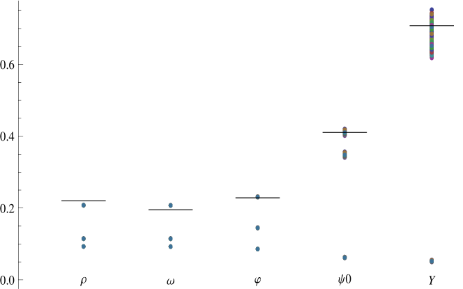
Figure 2: Amplitudes $f_{V}$ for all studied mesons are represented. Vertical scale is in units of Gev. Short horizontal lines are values obtained from experimental data. Lower sets of points are the NLO contributions obtained from our model. Intermediate sets of points are our LO results. Upper sets of points are our theoretical values of $f_{V}=f_{V}^{LO}+f_{V}^{NLO}$. It is concluded that same set of $A_{i}$ coefficients predicts simultaneously the $f_{V}$ for all five studied mesons and that uncertainties in the $A_{i}$ are strongly “amplified” for $Y$ and $\psi_{0}$.

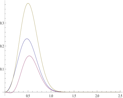
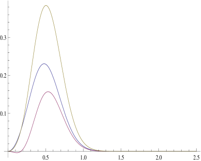
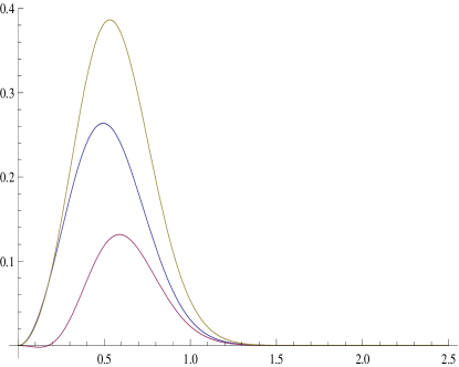
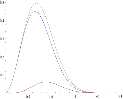
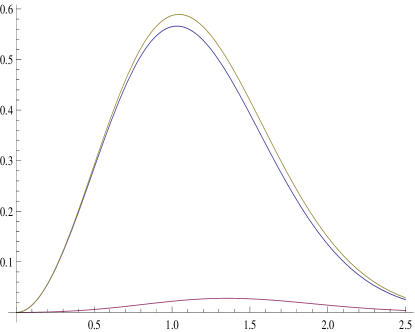
Figure 3: Plots of integrand functions which give rise to $f_{V}^{LO}$, $f_{V}^{NLO}$, and $f_{V}$, as functions of $\widehat{q}$, for the five vector mesons studied, respectively.

V Discussion

In this paper we have calculated the decay constants $f_{V}$ of vector mesons $\rho$, $\omega$, $\phi$, $\psi$ and $Y$ in BSE under Covariant Instantaneous Ansatz (CIA) using Hadron-quark vertex function which incorporates various Dirac covariants order-by-order in powers of inverse of meson mass within its structure in accordance with a recently proposed power counting rule from their complete set. This power counting rule suggests that the maximum contribution to any meson observable should come from Dirac structures associated with Leading Order (LO) terms alone, followed by Dirac structures associated with Next-to-Leading Order (NLO) terms in the vertex function. Incorporation of all these covariants is found to bring calculated $f_{V}$ values much closer to results of experimental data beringen12 and some recent calculations alkofer02 ; ivanov99 ; close02 ; li08 ; cvetic04 ; hwang97 ; alkofer01 ; wang08 for $\rho$, $\omega$, $\phi$, $\psi$ and $Y$ mesons. The $f_{V}$ predicted are within the error bars of experimental data for each one of these five mesons.

The results for $\rho$, $\omega$, $\phi$, $\psi$ and $Y$ mesons with parameter set: $A_{0}=1$, $A_{1}=0.007\pm 0.001$, $A_{2}=1.240\pm 0.001$, $A_{3}=-0.415\pm 0.001$, $A_{4}=0.014\pm 0.001$, $A_{5}=-1.842\pm 0.001$ (giving $f_{V}$ values with average error with respect to experimental data of 4%) are presented in Table 2. Comparison with experimental data and other models is shown in Table 2.

In Fig. 3 we are plotting vs $\hat{q}$ the integrands of $f^{LO}_{V}$, $f^{NLO}_{V}$ and $f_{V}$ for each of studied mesons. Those plots show that the contribution to $f_{V}$ from NLO covariants is smaller than the contribution from LO covariants for $\rho$, $\omega$, $\phi$, $\psi$ and $Y$ mesons. And for $\psi$ and $Y$ mesons, NLO contribution is negligible in comparison to LO contribution. Then, it is concluded from Table 2 that as far as the various contributions to decay constants $f_{V}$ are concerned, for $\rho$ and $\omega$ mesons, the LO terms contribute only  55%, while NLO terms  45%. However as one goes to $\phi$ meson, the LO contribution increases to  62.8%, while NLO contribution is 37.2%. But as one goes to heavy ($c\overline{c}$ and $b\overline{b}$) mesons, for $\psi$ meson, LO contribution is 84.8%, while NLO contribution is 15.2%, and for $Y$ meson the LO contribution is 92.6%, while NLO contribution reduces to just 7.4%. Thus the drop in contribution to decay constants from NLO covariants vis-a-vis LO covariants is more pronounced for heavy mesons $\psi$ and $Y$. And among the two LO covariants, it can be seen that the most leading covariant $i\gamma_{\mu}$ contributes the maximum for all vector mesons from $\rho$ to $Y$. These results on decay constants $f_{V}$ for vector mesons are completely in conformity with the corresponding results on decay constants $f_{P}$ for pseudoscalar mesons, $K,D,D_{S}$ and $B$ done recentlybhatnagar11 where it was also noticed that the NLO contribution is much smaller than the LO contribution for hevier mesons like $D,D_{S}$ and $B$, where the contribution drops from 10% to 4%, and the most leading covariant was found to be $\gamma_{5}$.

This is in conformity with the power counting rule according to which the leading order covariants, $\gamma_{5}$ and $i\gamma_{5}(\gamma\cdot P)(1/M)$ (associated with coefficients $A_{0}$ and $A_{1}$) should contribute maximum to decay constants followed by the next-to-leading order covariants, $-i\gamma_{5}(\gamma\cdot q)(1/M)$ and $-\gamma_{5}[(\gamma\cdot P)(\gamma\cdot q)-(\gamma\cdot q)(\gamma\cdot P)](1/M^{2})$ (associated with coefficients $A_{2}$ and $A_{3}$) in the BS wave function.

We observe in Fig. 2 that though LO and NLO Dirac covariants are sufficient to correctly predict amplitudes for $\phi$ and $\psi_{0}$ vector mesons, but only LO covariants are sufficient for $Y$ meson. But for $\rho$ and $\omega$ mesons, the LO and NLO Dirac covariants are not sufficient to predict accurately their amplitudes and is thus necessary to include even higher order NNLO Dirac covariants in their hadron-quark vertex functions. This can also be seen from Fig. 3.

However, the numerical results for $f_{V}$ for equal mass vector mesons, obtained in our framework with use of leading order Dirac covariants along with the next to leading order Dirac covariants, along with a similar calculation for $f_{P}$ done recently bhatnagar11 for pseudoscalar mesons demonstrates the validity of our power counting rule, which also provides a practical means of incorporating various Dirac covariants in the BS wave function of a hadron. By this rule, we also get to understand the relative importance of various covariants to calculation of meson observables. This would in turn help in obtaining a better understanding of the hadron structure.

References

• (1) R.Alkofer, P.Watson, H.Weigel, Phys. Rev. D65, 094026 (2002).
• (2) M.A.Ivanov, Yu A. Kalinovski, C.D. Roberts, Phys. Rev. D60, 034018 (1999).
• (3) F.E.Close, A.Donnachi, Yu S. Kalashnikova, Phys. Rev. D65, 092003 (2002).
• (4) H-M.Li, S-L.Wan, Chin. Phys. Lett. 25, 1239 (2008).
• (5) G.Cvetic et al., Phys. Lett. B596, 84 (2004).
• (6) D.S.Hwang, G.H.Kim, Phys. Rev. D55, 6944 (1997).
• (7) R.Alkofer, L.W.Smekel, Phys. Rep. 353, 281 (2001).
• (8) G.L.Wang, Intl. J. Mod. Phys. A23, 3263 (2008).
• (9) A. N. Mitra, B. M. Sodermark, Nucl. Phys. A695, 328 (2001) and references therein.
• (10) A.N.Mitra, PINSA 65, 527 (1999).
• (11) S. Bhatnagar, D. S. Kulshreshtha, A. N. Mitra, Phys. Lett. B263, 485 (1991).
• (12) A. N. Mitra, S. Bhatnagar, Intl. J. Mod. Phys. A7, 121 (1992).
• (13) S.Bhatnagar, S-Y. Li, J. Phys. G32, 949 (2006)
• (14) S. Bhatnagar, S-Y.Li, J. Mahecha, Intl. J. Mod. Phys. E20,1437 (2011).
• (15) C.H.L.Smith, Ann. Phys. 53, 521 (1969).
• (16) F.T.Hawes, M.A.Pichowsky, arxiv:nucl-th/9806025, 1998.
• (17) E.Mengesha, S.Bhatnagar, Intl. J. Mod. Phys. E20, 2521 (2011).
• (18) S.Bhatnagar, Intl. J. Mod. Phys. E14, 909 (2005).
• (19) K.K.Gupta et al., Phys. Rev. D42, 1604 (1990).
• (20) S.Bhatnagar and S.Y.Li, In the Proceedings of 9th Workshop on Non-Perturbative Quantum Chromodynamics, Paris, France, 4-8 Jun 2007, pp 12.
• (21) D.Arndt, C-R.Ji, Light-Cone Quark Model Analysis of Radially Excited Pseudoscalar and Vector Mesons. arXiv:hep-ph/9905360v1, 1999.
• (22) J.Beringen et al., (Particle Data Group), Phys. Rev. D86, 010001 (2012).