Integrable Boundary for Quad-Graph Systems

Integrable Boundary for Quad-Graph Systems:
Three-Dimensional Boundary Consistency

Vincent CAUDRELIER ^†, Nicolas CRAMPÉ ^‡ and Qi Cheng ZHANG ^†

V. Caudrelier, N. Crampé and Q.C. Zhang

^† Department of Mathematical Science, City University London,
^† Northampton Square, London EC1V 0HB, UK v.caudrelier@city.ac.uk, c.zhang@leeds.ac.uk

^‡ CNRS, Laboratoire Charles Coulomb, UMR 5221,
^‡ Place Eugène Bataillon – CC070, F-34095 Montpellier, France nicolas.crampe@um2.fr

Received July 19, 2013, in final form February 05, 2014; Published online February 12, 2014

We propose the notion of integrable boundary in the context of discrete integrable systems on quad-graphs. The equation characterizing the boundary must satisfy a compatibility equation with the one characterizing the bulk that we called the three-dimensional (3D) boundary consistency. In comparison to the usual 3D consistency condition which is linked to a cube, our 3D boundary consistency condition lives on a half of a rhombic dodecahedron. The We provide a list of integrable boundaries associated to each quad-graph equation of the classification obtained by Adler, Bobenko and Suris. Then, the use of the term “integrable boundary” is justified by the facts that there are Bäcklund transformations and a zero curvature representation for systems with boundary satisfying our condition. We discuss the three-leg form of boundary equations, obtain associated discrete Toda-type models with boundary and recover previous results as particular cases. Finally, the connection between the 3D boundary consistency and the set-theoretical reflection equation is established.

discrete integrable systems; quad-graph equations; 3D-consistency; Bäcklund transformations; zero curvature representation; Toda-type systems; set-theoretical reflection equation

05C10; 37K10; 39A12; 57M15

1 Introduction

Discrete integrable systems arise from various motivations in applied or pure mathematics like the need to preserve integrability of certains continuous equations when performing numerical (and hence discrete) simulations or the theory of discrete differential geometry. In previous work concerning an important class of such systems known as integrable quad-graph equations [11], one of the original motivations was to study discrete differential geometry of surfaces. In this context, a general construction allows one to always obtain a discretization of the surface in terms of quadrilaterals [11], at least as long as one is only concerned with the bulk of the surface and does not worry about its boundary (if it has one). The vertices of the graph thus obtained can be seen as discrete space-time points where the field is attached. The dynamics of the field is then specified by an equation of motion involving the values of the field at the four vertices forming an elementary quadrilateral. Typically, this is of the form

$$Q(u_{00},u_{10},u_{01},u_{11};a,b)=0,$$ (1)

where $u_{00}$, $u_{10}$, $u_{01}$, $u_{11}$ are the values of the field at the vertices of the quadrilateral and $a$, $b$ are parameters (see l.h.s. of the Fig. 3).

There exist several integrability criteria that different authors use to characterize the notion of discrete integrability. Let us mention for instance algebraic entropy [10], singularity confinement [19] or the 3D consistency/consistency around the cube condition [11, 26]. The latter is deeply related to the notion of discrete Lax pair, discrete Bäcklund transformations and other classical notions of integrability and, combined with a few other assumptions, led to the important ABS classification of quad-graph equations [2]. This fact and the similarity of the above structures with those existing in the case of continuous integrable systems make it a popular criterion.

In this paper, we want to propose a way of defining an integrable discrete system on a quad-graph with boundary as arising from the discretization of a surface while taking into account its boundary. From the geometric point of view, this is a natural generalization of the discrete differential geometry motivation to the case of a surface with boundary. From the point of view of discrete integrable quad-graph equations, this then allows us to tackle the problem of formulating the analog of the 3D consistency condition together with its consequences, i.e. Bäcklund transformations and zero curvature formulation. We also introduce Toda-type systems with boundary through the three-leg form of integrable equations on quad-graphs and we recover the previous approach to boundary conditions for discrete integrable systems presented in [20].

We give a precise definition of the discretization procedure and of a quad-graph with boundary in Section 2.1. Then we show how to define a discrete system on it. In addition to the elementary quadrilateral and the corresponding equation of motion (1), the new crucial ingredient is an elementary triangle together with the corresponding boundary equation of the form

$$q(x,y,z;a)=0,$$

where $x$, $y$, $z$ are the values of the field at the vertices of the triangle, and a function $\sigma$ determining the effect of the boundary on the labelling (see r.h.s. of the Fig. 3). We provide our definition of integrability in this context by defining the 3D boundary consistency condition involving $Q$, $q$ and $\sigma$ in Section 2.3 and then go on to present a method that allows us to find solutions for $q$ and $\sigma$ for a given $Q$ in Section 3. In Section 4, we justify further our introduction of the 3D boundary consistency condition by discussing Bäcklund transformations and the zero curvature representation in the presence of a boundary. Section 5 introduces the three-leg form for boundary equations and we use this to define systems of Toda-type with boundary. As an example, we recover as particular case the approach to boundary conditions of [20] in (fully) discrete integrable systems. Finally, in Section 6 we establish the connection between the 3D boundary consistency condition introduced in this paper and the set-theoretical reflection equation [14, 15] in the same spirit [28] as the 3D consistency condition is related to the set-theoretical Yang–Baxter equation [17]. Conclusions and outlooks are collected in the last section.

2 Integrable quad-graph systems with boundary

In this section, we first define the notion of quad-graph with boundary and then use it to define the elementary blocks needed to study integrable equations on quad-graphs with boundary.

2.1 Quad-graph with boundary

Our starting point is the definition of a quad-graph from a cellular decomposition of an oriented surface ${\cal S}$ containing only quadrilateral faces. As explained in [11], a quad-graph can always be obtained from an arbitrary cellular decomposition ${\cal G}$ by forming the double ${\cal D}$ (in the sense of [11], otherwise called a diamond in [25]) of ${\cal G}$ and its dual cellular decomposition ${\cal G}^{*}$. So far, these notions apply to surfaces without a boundary. For the case of a surface with boundary, the notion of dual cellular decomposition does not exist in general. In [25], Definition 1 gives the definition of an object $\Gamma^{*}$ associated to a cellular decomposition $\Gamma$ of a compact surface with boundary and it is noted that $\Gamma^{*}$ is not a cellular decomposition of the surface. Nevertheless, in Section C.3 of [24], a notion of double is given for a surface with boundary (and not necessarily compact, like a half-plane) and we adapt it here for our purposes. In particular, we will see that the generic structure that arises is what we call a quad-graph with boundary with its faces being either quadrilaterals or “half quadrilaterals”, i.e. triangles.

So let us consider a cellular decomposition ${\cal G}$ of our surface ${\cal S}$ with a boundary. We denote, respectively, by $F$, $E$ and $V$ the set of faces, edges and vertices of this cellular decomposition. Following [24] and adapting slightly, we define ${\cal G}^{*}$ as the following collection of cells with $F^{*}$, $E^{*}$ and $V^{*}$ respectively the sets of faces, edges and vertices.

• To each face in $F$, we associate a vertex $v^{*}$ in $V^{*}$ (called white), placed inside the face.

• To each edge $e\in E$ not on the boundary, we associate the dual edge $e^{*}\in E^{*}$ which cuts it tranversally and forms a path between the two white vertices contained in the two adjacents faces in $F$ separated by $e$.

• To each vertex $v\in V$ (called black) not on the boundary, we associate the face in $F^{*}$ that contains it, i.e. the face whose boundary is made of the edges in $E^{*}$ that cross the edges in $E$ having the vertex $v$ under consideration as one of their ends.

Compared to Definition 6 of [24], in our definition of ${\cal G}^{*}$, we include neither the dual edge corresponding to an edge on the boundary nor the additional white vertex in the middle of an edge in $E$ belonging to the boundary. A typical configuration of ${\cal G}$ and ${\cal G}^{*}$ is shown in Fig. 1.

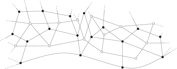
Figure 1: Example of a cellular decomposition ${\cal G}$ and of the associated ${\cal G}^{*}$. The “horizontal” curved line is the boundary of the underlying surface ${\cal S}$. The black dots and the straight lines connecting them are the vertices and edges of the initial cellular decomposition ${\cal G}$. The white dots and the straight lines connecting them are the vertices and edges of ${\cal G}^{*}$. Edges of ${\cal G}$ on the boundary and the boundary itself are identified in this picture.

We now form the structure that we will call a quad-graph with boundary below. Let us denote it ${\cal D}$. The vertices of ${\cal D}$ are all the black and white vertices, i.e. $V_{\cal D}=V\cup V^{*}$. The edges of ${\cal D}$ are all the edges in $E$ that lie on the boundary of ${\cal S}$ together with those edges $(w,b)$ obtained by connecting a white vertex to each of the black vertices sitting on the face that contains the white vertex. The faces are then taken to be the interiors of the “polygons” thus obtained. The result of this procedure for ${\cal G}$ and ${\cal G}^{*}$ as in Fig. 1 is shown in Fig. 2. The faces are therefore of two types:

• Quadrilaterals, with two black and two white vertices, in the bulk.

• Triangles, with two black vertices (on the boundary) and one white vertex (inside ${\cal S}$), alongside the boundary.

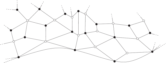
Figure 2: Example of a quad-graph with boundary ${\cal D}$. Black and white dots are the vertices of the double and the straight lines are edges. Edges of ${\cal G}$ on the boundary and the boundary itself are identified in this picture and form the rest of the edges of ${\cal D}$. Faces are therefore either quadrilaterals (with two black and two white alternating vertices) or triangles lying along the boundary (with two black vertices and one white vertex).

Definition 2.1.

A quad-graph with boundary is the collection of vertices and edges of ${\cal D}$ obtained as described above from a cellular decomposition of a surface with boundary.

As an important by-product, this procedure to get a quad-graph with boundary allows one to obtain a bipartite graph. In addition, all the vertices on the boundary are of the same type. This property will be important in the construction of the Toda models in Section 5.

2.2 Discrete equations on quad-graph with boundary

We are now ready to define discrete equations on a quad-graph with boundary. As usual, we associate a field to this quad-graph (i.e. a function from $V\cup V^{*}$, the set of vertices, to ${\mathbb{C}}$) and a constraint between the values of the field around a face. This constraint can be seen as the equation of motion for the field. For each quadrilateral face, the constraint is, as usual, defined by

$$Q(u_{00},u_{10},u_{01},u_{11};a,b)=0,$$ (2)

where $u_{00},u_{10},u_{01},u_{11}\in{\mathbb{C}}$ are the values of the field at each vertex around the face and $a,b\in{\mathbb{C}}$ are parameters associated to opposite edges. One usually represents this equation as on the l.h.s. of Fig. 3.

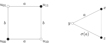
Figure 3: Elementary blocks to construct a discrete system with boundary.

We will refer to equation (2) as describing the bulk dynamics. Sometimes, one demands additional properties [11] for the function $Q(u_{00},u_{10},u_{01},u_{11};a,b)$ such as linearity on each variable $u_{00}$, $u_{10}$, $u_{01}$, $u_{11}$ (affine-linearity), symmetry by exchange of these variables ($D_{4}$-symmetry), the tetrahedron property or the existence of the three-leg form (see Section 5).

The new elementary building block needed to define a discrete system on a quad-graph with boundary is an equation of the following type defined on each triangular face

$$q(x,y,z;a)=0,$$ (3)

where $x$, $z$ are values of the field on the boundary, $y$ a value inside the surface and $a$ is a parameter associated to one edge (the other edge is associated to a function $\sigma(a)$ of the parameter $a$). We represent this equation as on the r.h.s. of Fig. 3 where the dashed line represents the edge on the boundary of the surface. We will refer to this equation as describing the boundary dynamics. In general, there is no special requirement on $q$ or $\sigma$ but we will see that our methods to construct expressions for $q$ result in $q$ having certain properties:

• Linearity: the function $q(x,y,z;a)$ is linear in the variables $x$ and $z$. Let us emphasize that it may not be linear in $y$.

• Symmetry: one has $\sigma(\sigma(a))=a$ and

  $$q(x,y,z;a)=0\quad\Leftrightarrow\quad q(z,y,x;\sigma(a))=0.$$

• In some cases, a three-leg form for $q$ inherited from the three-leg form of the corresponding bulk equation $Q=0$. We go back to this point in Section 5.

Let us remark that for a given quad-graph with boundary (and for $\sigma$ being not the identity), it is not always possible to label the edges with parameters as prescribed above. We show on the l.h.s. of Fig. 4 a quad-graph with boundary for which we cannot find a suitable labelling. On the r.h.s., we show a case where this is possible. In the following, we consider only those quad-graph with boundary that can be labelled. It would be very interesting to study this combinatorial problem in general but this goes beyond the scope of this paper.

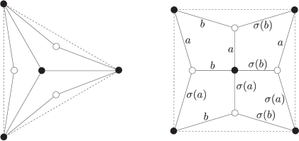
Figure 4: Two examples of quad-graphs with boundary (represented by a dashed line here). Only the one of the right-hand side can be labelled according to our rules for quadrilaterals and triangles.

2.3 Integrability: the 3D boundary consistency condition

As explained in the introduction, we adopt the 3D consistency approach to integrable quad-graph equations. Let us first recall what it means in the bulk case [11, 26] before we introduce its boundary analog. The usual setup is depicted in l.h.s. of Fig. 5 where the bulk equation of motion $Q=0$ is attached to each face of the cube. Given values of the field in the three independent directions of the cube, say $u_{000}$, $u_{100}$, $u_{010}$, $u_{001}$, there are three different ways of computing $u_{111}$ by repeated use of $Q=0$. The 3D consistency condition requires that these three possibilities give the same result for $u_{111}$.

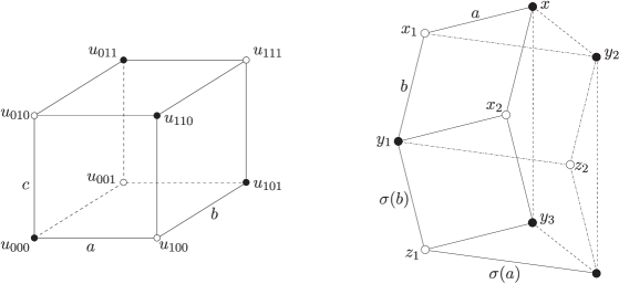
Figure 5: 3D consistency and 3D boundary consistency. We recall that parallel edges carry the same parameter.

We propose, in the following, the main new equation of this article which is a similar consistency condition for the function $q$ (and $\sigma$) that we call the 3D boundary consistency condition. This condition is in fact a compatibility condition between the bulk equation $Q=0$ and the boundary equation $q=0$. Instead of the cube for the 3D consistency, the 3D boundary consistency lies on a half of a rhombic dodecahedron as displayed in r.h.s. of Fig. 5. Let us remark that this half of a rhombic dodecahedron has the same combinatorial structure than the r.h.s. of the Fig. 4. On each face (resp. 4 quadrilaterals and 4 triangles), we attach its corresponding equation of motion (resp. $Q=0$ and $q=0$). Then, the 3D boundary consistency is the statement that, given the values $x$, $x_{1}$ and $x_{2}$ of the field, the different schemes to compute $w$ (see Fig. 5) lead to the same results. More precisely, following the notations in Fig. 5, we get that, given $x$, $x_{1}$ and $x_{2}$:

• the three equations

  $$Q(y_{1},x_{2},x_{1},x;a,b)=0,\qquad q(x,x_{1},y_{2};a)=0,\qquad q(x,x_{2},y_{3};b)=0,$$ (4)

  gives respectively the values of $y_{1}$, $y_{2}$ and $y_{3}$.

• Then, both equations

  $$Q(y_{1},z_{1},x_{2},y_{3};\sigma(b),a)=0,\qquad Q(y_{1},z_{2},x_{1},y_{2};\sigma(a),b)=0,$$ (5)

  gives respectively the values of $z_{1}$ and $z_{2}$.

• Finally, the three equations

  $$q(y_{2},z_{2},w;b)=0,\qquad q(y_{3},z_{1},w;a)=0,\qquad Q(y_{1},z_{1},z_{2},w;\sigma(b),\sigma(a))=0,$$ (6)

  provides three ways to compute $w$ which must give the same answer.

Definition 2.2.

We say that we solve the 3D boundary consistency for $q$ if, given a 3D consistent $Q$, we find a function $q$ of $x$, $y$, $z$, $a$ and a function $\sigma$ of $a$ such that the scheme (4)–(6) gives a unique value for $w$ given values for $x$, $x_{1}$ and $x_{2}$. In this case, $q$ is called a solution of the 3D boundary consistency condition (we omit explicit reference to $\sigma$ which is taken as part of the solution). We also say that $q$ is compatible with $Q$.

Note that this should not be confused with the notion of a solution of the actual dynamics described by $Q$ and $q$. Such a solution would consists in finding an expression for the field $u$ at each vertex of the quad-graph that satisfies the bulk and boundary dynamics. This is an exciting open question which deserves separate attention and is beyond the scope of the present paper.

In the bulk case, when one finds a $Q$ which satisfies the 3D consistency (see Fig. 5), the associated system is called an integrable equation on quad-graph [2, 11, 26]. To introduce a boundary which preserves the integrability, for a given $Q$, we must solve the 3D boundary consistency condition, i.e. find compatible functions $q$ and $\sigma$.

Definition 2.3.

We call integrable equation on a quad-graph with boundary the data of a quad-graph with boundary with compatible labelling as well as functions $Q$, $q$ and $\sigma$ which satisfy the 3D consistency and the 3D boundary consistency conditions.

We justify the adjective “integrable” in Sections 4.1 and 4.2 by showing the presence of Bäcklund transformations and a zero curvature representation.

Let us emphasize that similar approaches have already appeared in the literature to introduce integrable boundaries in different contexts. Indeed similar figures to those in Fig. 5 appeared in [4, 9, 18] as the face representation of the reflection equation [16, 30]. The right-hand-side of Fig. 5 is also half of the figure representing the tetrahedron equation [7, 8]. There exists also a close connection between the set-theoretical equation introduced recently in [14, 15] and the 3D boundary consistency (see Section 6 for more details). Similar connections have been studied previously in the bulk case where the set-theoretical Yang–Baxter equation is linked to the 3D consistency condition [2, 28].

3 Solutions of the 3D boundary consistency

In this section, we provide a list of solutions of the 3D boundary consistency condition associated to the bulk equations $Q$ classified in [2]. In other words, given $Q$, we want to find solutions $q$ and $\sigma$ which satisfy the 3D boundary consistency conditions. The underlying idea is that this should provide integrable boundary conditions for integrable discrete equations characterized by $Q$.

3.1 The ABS classification

For completeness, we list the solutions of the 3D consistency equations (2) obtained in [2]

$${\rm(Q1)}:\quad a(u_{00}-u_{01})(u_{10}-u_{11})-b(u_{00}-u_{10})(u_{01}-u_{11})+\delta^{2}ab(a-b)=0,$$

$${\rm(Q2)}:\quad a(u_{00}-u_{01})(u_{10}-u_{11})-b(u_{00}-u_{10})(u_{01}-u_{11})$$

$${}+ab(a-b)(u_{00}+u_{10}+u_{01}+u_{11})-ab(a-b)\big{(}a^{2}-ab+b^{2}\big{)}=0,$$

$${\rm(Q3)}:\quad \big{(}b^{2}-a^{2}\big{)}(u_{00}u_{11}+u_{10}u_{01})+b\big{(}a^{2}-1\big{)}(u_{00}u_{10}+u_{01}u_{11})$$

$${}-a\big{(}b^{2}-1\big{)}(u_{00}u_{01}+u_{10}u_{11})-\delta^{2}\big{(}a^{2}-b^{2}\big{)}\big{(}a^{2}-1\big{)}\big{(}b^{2}-1\big{)}/(4ab)=0,$$

$${\rm(Q4)}:\quad \operatorname{sn}(a)(u_{00}u_{10}+u_{01}u_{11})-\operatorname{sn}(b)(u_{00}u_{01}+u_{10}u_{11})-\operatorname{sn}(a-b)(u_{00}u_{11}+u_{10}u_{01})$$

$${}+\operatorname{sn}(a-b)\operatorname{sn}(a)\operatorname{sn}(b)(1+K^{2}u_{00}u_{10}u_{01}u_{11})=0,$$

$${\rm(H1)}:\quad (u_{00}-u_{11})(u_{10}-u_{01})+b-a=0,$$

$${\rm(H2)}:\quad (u_{00}-u_{11})(u_{10}-u_{01})+(b-a)(u_{00}+u_{10}+u_{01}+u_{11})+b^{2}-a^{2}=0,$$

$${\rm(H3)}:\quad a(u_{00}u_{10}+u_{01}u_{11})-b(u_{00}u_{01}+u_{10}u_{11})+\delta^{2}\big{(}a^{2}-b^{2}\big{)}=0,$$

$${\rm(A1)}:\quad a(u_{00}+u_{01})(u_{10}+u_{11})-b(u_{00}+u_{10})(u_{01}+u_{11})-\delta^{2}ab(a-b)=0,$$

$${\rm(A2)}:\quad b\big{(}a^{2}-1\big{)}(u_{00}u_{01}+u_{10}u_{11})-a\big{(}b^{2}-1\big{)}(u_{00}u_{10}+u_{01}u_{11})$$

$${}+\big{(}b^{2}-a^{2}\big{)}(u_{00}u_{10}u_{01}u_{11}+1)=0.$$

We use the same labels (Q, H, A families) and forms that were used in [2], except for equation (Q4) which is in an equivalent form introduced in [5, 21] where $\operatorname{sn}(a)=\operatorname{sn}(a;K)$ is the Jacobi elliptic function with modulus $K$. It is worth noting that the 3D consistency condition as well as the affine-linearity, $D_{4}$-symmetry and tetrahedron properties are preserved for each of the equations up to common Möbius transformations on the variables $u_{00}$, $u_{10}$, $u_{01}$, $u_{11}$ and point transformations on the parameters $a$, $b$.

3.2 Method and solutions

Instead of performing brute force calculations where one could make assumption on the form of $q$ (like multilinearity in the variables) and insert in the 3D boundary consistency condition for a given $Q$, below we describe a simple method that amounts to “fold”, in a certain sense, $Q$ to obtain compatible $q$’s. Although it may seem ad hoc and arbitrary, this method has several motivations. First, it gives a simple way to obtain three-leg forms for $q$ knowing the ones for $Q$ and hence a way to introduce discrete Toda-type systems with boundary. This is explained in Section 5. Second, the method is a simple adaptation of the folding method that was used in [14] to obtain reflection maps, i.e. solutions of the set-theoretical reflection equation. This last point is discussed in more detail in Section 6. There, we present an alternative method to find admissible $q$’s starting from reflection maps. This alternative method produces some of the solutions that are also obtained with the method that we explain here. But more importantly, this alternative method establishes a deep connection between solutions of the 3D boundary consistency condition and reflection maps. This is reminiscent of the deep connection between solutions $Q$ of the 3D consistency condition (in particular the ones of the ABS classification) and quadrirational Yang–Baxter maps [3].

Now, given $Q$ satisfying the 3D consistency condition, we look for $q(u_{00},u_{10},u_{11};a)$ of the form

$$q(u_{00},u_{10},u_{11};a)=Q(u_{00},u_{10},k(u_{00},u_{10};a),u_{11};a,\sigma(a)),$$ (7)

satisfying the 3D boundary consistency condition, where $k$ and $\sigma$ are the functions to be determined. Equation (7) may be seen as the folding along the diagonal $(u_{00},u_{11})$ of the quadrilateral in Fig. 3 to get the triangle $(u_{00},u_{10},u_{11})$. Obviously, one may fold along the other diagonal but, due to the $D_{4}$-symmetry of $Q$, we get the same results.

To find $k$ and $\sigma$ (and hence $q$), for each given $Q$, we insert our ansatz (7) in the scheme (4)–(6) and try to find functions $k$ and $\sigma$ that fulfill the resulting constraints. We note that the following “trivial” choice

$$\sigma(a)=a,\qquad k(u_{00},u_{10};a)=-u_{10},$$ (8)

is always a solution of the problem for any $Q$. It yields $q(u_{00},u_{10},u_{11};a)=au_{10}(u_{00}-u_{11})$. We report in Tables 1 and 2 the nontrivial functions $k$, $\sigma$ and $q$ we found for the different $Q$’s of the Q, H and A families of the ABS classification. Note that we make no claim of completeness. A method for a systematic classification is in fact an interesting open problem.

Table 1: Results for boundary equations (Q family). $\mu$ is a free parameter. The asterisk denotes solutions that are also obtained with the method of Section 6.

2pt2pt ABS	$\sigma(a)$	$q(x,y,z;a)$	$k(x,u;a)$
Q1δ=0	$\frac{\mu^{2}}{a}^{*}$	$a(y-z)+\mu(x-y)$	$x+\frac{\mu}{a}(x-u)$4pt2pt
	$\frac{\mu^{2}}{a}^{*}$	$ax(y-z)+\mu z(y-x)$	$\frac{axu}{au+\mu(x-u)}$2pt
	$-a+2\mu^{*}$	$y(x+z)$	$\frac{\mu xu+(a-\mu)x^{2}}{(a-\mu)u+\mu x}$2pt
	$-a+2\mu^{*}$	$a\left(y^{2}-xz\right)+(x-y)(y+z)\mu$	$-u$2pt
Q1δ=1	$\frac{\mu^{2}}{a}^{*}$	$a(y-z-\mu)\pm\mu(y-x-\mu)$	$x+\mu\pm\frac{\mu}{a}(u-x-\mu)$4pt2pt
	$-a+2\mu^{*}$	$y(x-z)$	$x+\frac{a(a-2\mu)}{x-u}$2pt
	$-a+2\mu^{*}$	$(y-x)(y-z)+a(a-2\mu)$	$u$2pt
	$-a+2\mu$	$y(x+z)$	$\frac{x(ax-\mu(x-u))-a(a-\mu)(a-2\mu)}{au+\mu(x-u)}$2pt
	$-a+2\mu$	$(y^{2}-xz)+\frac{\mu}{a}(x-y)(y+z)$	$-u$2pt
		$\quad{}-(a-\mu)(a-2\mu)$	2pt
Q3δ=0	$\pm\frac{\mu}{a}^{*}$	$y(x\pm z)$	$\pm\frac{((a^{2}-\mu)x-a(1-\mu)u)x}{(a^{2}-\mu)u-a(1-\mu)x}$4pt2pt
	$\pm\frac{\mu}{a}^{*}$	$(a^{2}+\mu)\left(y^{2}\pm xz\right)$	$\pm u$2pt
		$\quad{}-a(1+\mu)y(x\pm z)$	2pt
	$-a$	$y(x+z)$	$-u$2pt
Q3δ=1	$\frac{\mu}{a}$	$y(x\pm z)$	$\frac{a(\mu\mp 1)xu-(\mu\mp a^{2})x^{2}+\frac{1}{4}(a^{2}-1)(a^{2}-\mu^{2})\left(\frac{1}{\mu}\mp\frac{1}{a^{2}}\right)}{(a^{2}\mp\mu)u-a(1\mp\mu)x}$6pt2pt
	$\frac{\mu}{a}$	$a(\mu\pm 1)y(x\pm z)$	$\pm u$2pt
		$\quad{}-(\mu\pm a^{2})(y^{2}\pm xz)$	2pt
		$\quad{}+\frac{1}{4}(\frac{1}{\mu}\pm\frac{1}{a^{2}})(a^{2}-1)(a^{2}-\mu^{2})$	2pt
	$-a$	$y(x+z)$	$-u$2pt
Q4	$-a$	$y(x+z)$	$\frac{x^{2}-\operatorname{sn}^{2}(a)}{u(1-K^{2}\operatorname{sn}^{2}(a)x^{2})}$4pt2pt
	$-a$	$\operatorname{sn}^{2}(a)(K^{2}y^{2}xz-1)+y^{2}-xz$	$-u$2pt

Table 2: Results for boundary equations (H and A families). $\mu$ is a free parameter. The asterisk denotes solutions that are also obtained with the method of Section 6.

ABS	$\sigma(a)$	$q(x,y,z;a)$	$k(x,u;a)$2pt2pt
H1	$-a+2\mu^{*}$	$y(x+z)$	$u+\frac{\mu-a}{x}$2pt2pt
	$-a+2\mu^{*}$	$y(z-x)+a-\mu$	$-u$2pt
H2	$-a+\mu^{*}$	$x+2y+z+\mu$	$u$2pt2pt
	$-a+\mu^{*}$	$y(z-x)$	$-2x-u-\mu$2pt
	$-a+\mu$	$2y(x-z)+(\mu-2a)(x+z+\mu)$	$-u$2pt
	$-a+\mu$	$y(x+z)$	$\frac{2ux+(u+\mu)(\mu-2a)}{2x+2a-\mu}$2pt
H3δ=0	$-a$	$y(x+z)$	$-u$2pt2pt
	$\frac{\mu}{a}$	$y(x\pm z)$	$\pm u$2pt
H3δ=1	$\frac{\mu}{a}^{*}$	$y(x\pm z)$	$\pm u-\frac{\mu\mp a^{2}}{ax}$6pt2pt
	$\frac{\mu}{a}^{*}$	$a^{2}+ay(x\pm z)\pm\mu$	$\pm u$2pt
	$-a$	$y(x+z)$	$-u$2pt
A1δ=0	$\frac{\mu^{2}}{a}^{*}$	$\mu(x+y)+a(y+z)$	$-x+\frac{\mu}{a}(u+x)$6pt2pt
	$\frac{\mu^{2}}{a}^{*}$	$ax(y+z)+(x+y)z\mu$	$\frac{axu}{\mu(u+x)-au}$2pt
	$-a+2\mu^{*}$	$y(x+z)$	$\frac{(ax-\mu(u+x))x}{au-\mu(u+x)}$2pt
	$-a+2\mu^{*}$	$a\left(y^{2}-xz\right)-(x+y)(y-z)\mu$	$-u$2pt
A1δ=1	$\frac{\mu^{2}}{a}^{*}$	$a(y+z-\mu)\pm\mu(x+y-\mu)$	$-x+\mu\pm\frac{\mu}{a}(x+u-\mu)$2pt2pt
	$-a+2\mu^{*}$	$y(z-x)$	$-x-\frac{a(a-2\mu)}{x+u}$2pt
	$-a+2\mu^{*}$	$(x+y)(y+z)+a(a-2\mu)$	$u$2pt
	$-a+2\mu$	$y(x+z)$	$\frac{x(ax-\mu(x+u))-a(a-\mu)(a-2\mu)}{au-\mu(x+u)}$2pt
	$-a+2\mu$	$\frac{\mu}{a}(x+y)(y-z)-\left(y^{2}-xz\right)+(a-\mu)(a-2\mu)$	$-u$2pt
A2	$\pm\frac{\mu}{a}^{*}$	$y(z\pm x)$	$\pm\frac{a(\mu-1)ux+a^{2}-\mu}{(a^{2}-\mu)xu+a(\mu-1)}$6pt2pt
	$\pm\frac{\mu}{a}^{*}$	$a(1+\mu)y(x\pm z)-(a^{2}+\mu)\left(1\pm xy^{2}z\right)$	$\pm u$2pt
	$-a$	$y(z+x)$	$-u$2pt

4 Other aspects of integrable equations on quad-graphs
with boundary

In this section, we present results on important traditional aspects of integrability obtained from the 3D boundary consistency equation. They justify a posteriori our definition of integrability for quad-graphs with boundary.

4.1 Bäcklund transformations

In this subsection, we prove that the 3D boundary consistency condition proposed in the previous section leads naturally to Bäcklund transformations which are a basic tool in the context of classical integrability and soliton theory. This result is similar to the one without boundary [2] and is summarized in the following proposition:

Proposition 4.1.

Let us suppose that we have an integrable equation on a quad-graph with boundary $($with the set of all its vertices denoted as $V)$ as well as a solution, $g:V\rightarrow{\mathbb{C}}$. There exist a two-parameter solution $g^{+}$ of the same integrable quad-graph equation and a function $f$ from $V$ to ${\mathbb{C}}$ satisfying

$$Q(g(v),g(v_{1}),f(v),f(v_{1});a,\lambda)=0,\qquad Q\big{(}f(v),f(v_{1}),g^{+}(v),g^{+}(v_{1});a,\sigma(\lambda)\big{)}=0,$$

for all edges $(v,v_{1})$ of the quad-graph not on the boundary of the surface $(a$ is the parameter associated to this edge$)$, and

$$q\big{(}g(v_{2}),f(v_{2}),g^{+}(v_{2});\lambda\big{)}=0,$$

for all vertices $v_{2}$ on the boundary of the quad-graph. We call the solution $g^{+}$ the Bäcklund transform of $g$.

Proof 4.2.

The proof follows the same lines as in the case without boundary. We start with the quad-graph with boundary, called in this proof the ground floor. We consider also two other copies of the surface, called first and second floor, of the ground floor. Then, we construct a 3D graph by the following procedure (see also Fig. 6):

• There is a one-to-one correspondence between the vertices of the ground floor and the ones of the first floor but one moved the vertices of the first floor such that no vertex of the first floor lies on the boundary of the surface (see l.h.s. of the Fig. 6). The vertices on the second floor is an exact copy of the ones on the ground floor.

• We copy the edges in the bulk of the ground floor on the first and second floor. The copies carry the same label. We copy the edges on the boundary of the ground floor only on the second floor.

• We add the edges (thin lines on the Fig. 6) linking all the vertices of the ground floor with the corresponding vertices of the first floor and similarly from the first to the second floor. The edges between the ground and first floor carry the label $\lambda$ whereas the edges between the first and second floor carry $\sigma(\lambda)$. We add also the edges between the vertices on the boundary of the ground floor to the corresponding ones on the second floor.

• the set of faces is the union of the following sets: (i) the triangular and quadrilateral faces of the ground and second floor; (ii) the quadrilateral faces of the first floor; (iii) the “vertical” quadrilateral faces made from the edges of the ground floor, the corresponding ones of the first floor and the vertical edges linking the vertices of these edges, and similarly between the first and second floors; (iv) the “vertical” triangular faces made of the edges linking the vertices on the boundary of the ground and second floors and the corresponding vertex of the first floor (which is not on the boundary).

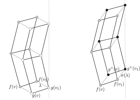
Figure 6: The figure on the left shows the ground floor (white vertices and thick lines connecting them) and the first floor (gray vertices and thick lines connecting them) corresponding to a typical configuration near the boundary. The first floor and the second one (black vertices and thick lines connecting them) is shown on the figure on the right. The thin lines correspond to the edges linking the different floors: they carry $\lambda$ on the left and $\sigma(\lambda)$ on the right.

We impose now that the values of the field living on this 3D graph be constrained by $Q=0$ on each quadrilateral face and by $q=0$ on each triangular faces.

As in the case without boundary, due to the 3D consistency condition, given a function $g$ satisfying the constraints on the ground floor, one can get a function $f$ satisfying the constraint on the first floor depending on $\lambda$ and on the value of $f$ at one vertex of the first floor. This function $f$ satisfies, in particular, $Q(g(v),g(v_{1}),f(v),f(v_{1});a,\lambda)=0$.

Knowing the value of the field at one vertex on the boundary of the ground floor (say $g(v_{1})$ on the figure) and the corresponding value on the first floor ($f(v_{1})$), we get the value $g^{+}(v_{1})$ of the field $g^{+}$ at the corresponding vertex of the second floor using the equation $q(g(v_{1}),f(v_{1}),g^{+}(v_{1})$, $\lambda)=0$ which connects the white, grey and black copies of the vertex $v_{1}$.

We obtain a function $g^{+}$ satisfying the constraints of the second floor using $Q$ on the “vertical” quadrilateral faces between the first and second floors. The important point is to remark that due to the 3D consistency and the 3D boundary consistency conditions, all the different ways to obtain the values of $g^{+}$ give the same result. We may see this geometrically since the only “elementary blocks” of the 3D graph are cubes or half of rhombic dodecahedron and since the functions $Q$ and $q$ are chosen such that they satisfy the 3D consistency and the 3D boundary consistency conditions, the different ways to compute the values of the field $g^{+}$ are consistent.

Finally, using the fact that the second floor is an exact copy of the ground floor, $g^{+}$ satisfies the constraints of the original quad-graph equations.

Let us remark that the main difference between the cases with and without boundary lies in the necessity of an additional, intermediate floor in the case with boundary. This feature appeared previously in the context of asymmetric quad-graph equations [13]. Let us emphasize that the function $f$ defined on the intermediate floor is not in general a solution of the same equations on a quad-graph with boundary since the values of the field on the vertices of the “would-be” boundary of the first floor do not necessarily satisfy an equation of the type (3).

4.2 Zero curvature representation

It is well established that a 3D consistent system $Q(u_{00},u_{10},u_{01},u_{11};a,b)$ admits a zero curvature representation [11, 12, 26], i.e. there exists a matrix $L$ depending on values of the field on the same edge, the parameter associated to this edge and a spectral parameter $\lambda$ such that the following equation holds

$$L(u_{11},u_{10},b;\lambda)~{}L(u_{10},u_{00},a;\lambda)~{}=~{}L(u_{11},u_{01},a;\lambda)~{}L(u_{01},u_{00},b;\lambda).$$ (9)

There exists a constructive way to get $L$ from $Q$ [11, 26]: due to the linearity of the function $Q$, we can rewrite equivalently equation (2) as follows

$$u_{11}=L(u_{10},u_{00},a;b)[u_{01}],$$ (10)

where $L$ is a 2 by 2 matrix describing, with usual notations, a Möbius transformation

$$L[z]=\frac{\alpha z+\beta}{\gamma z+\delta}\qquad\text{where}\qquad L=\left(\begin{matrix}\alpha&\beta\\ \gamma&\delta\end{matrix}\right).$$

Geometrically, using Fig. 5, it is easy to show that the matrix (10) satisfies the zero curvature equation (9) if $Q$ satisfies the 3D consistency [11, 12, 26].

Similarly, we want to show that the 3D boundary consistent system admits a zero curvature representation. For the boundary equation $q(x,y,z;a)=0$, we propose the following zero curvature representation

$$K(z;c)L(z,y,\sigma(a);c)L(y,x,a;c)=L(z,y,\sigma(a);\sigma(c))L(y,x,a;\sigma(c))K(x;c),$$ (11)

where $K$ is also a 2 by 2 matrix. We can now state the following results justifying the previous definition:

Proposition 4.3.

All the examples of boundary equations $q(x,y,z;a)=0$ displayed in Tables 1 and 2 as well as the trivial solution (8) can be represented by equation (11) where $K(x;a)[u]$ is the $2$ by $2$ matrix describing the function $k(x,u;a)$, understood as a Möbius transformation w.r.t. $u$ with polynomial coefficients in $x$ and $a$.

Proof 4.4.

We give the details of the proof for the case given in the first row of the Table 1, i.e. we deal with the bulk equation ${\rm Q1}_{\delta=0}$ given by

$$Q(u_{00},u_{10},u_{01},u_{11};a,b)=a(u_{00}-u_{01})(u_{10}-u_{11})-b(u_{00}-u_{10})(u_{01}-u_{11}),$$

and the boundary equation characterized by

$$q(x,y,z;a)=a(y-z)+\mu(x-y)\qquad\text{with}\quad\sigma(a)=\frac{\mu^{2}}{a},$$

$$k(x,u;a)=\frac{-\mu u+x(\mu+a)}{a}.$$ (12)

The matrix $L$ associated to this $Q$ is given by

$$L(y,x,a;b)=\frac{1}{\sqrt{b}\sqrt{b-a}(x-y)}\left(\begin{matrix}ay+b(x-y)&-axy\\ a&-ax+b(x-y)\end{matrix}\right).$$

It is a known result that equation (9) with this choice for $L$ is satisfied if $Q(u_{00},u_{10},u_{01},u_{11};a,b)$ $=0$ but it is easily verified. Let us mention that the parameters entering in the square roots of the normalisation of $L$ may be negative. Therefore, one must choose a branch cut for the square root appearing in the normalisation: we choose the half-line $\{ix\,|\,x<0\}$.

The matrix $K$ associated to the function $k$ given by (12) is

$$K(x;a)=\left(\begin{matrix}-1&\big{(}\frac{a}{\mu}+1\big{)}x\\ 0&\frac{a}{\mu}\end{matrix}\right).$$

By algebraic computation, one gets

$$K(z;c)~{}L(z,y,\sigma(a);c)~{}L(y,x,a;c)-L(z,y,\sigma(a);\sigma(c))~{}L(y,x,a;\sigma(c))~{}K(x;c)$$

$$\qquad\propto q(x,y,z;a)\left(\begin{matrix}a(y-z)&-ax(y-z)+cz(y-x)\\ 0&c(y-x)\end{matrix}\right).$$

Therefore, if $q(x,y,z;a)=0$, relation (11) holds. That proves the proposition for this case. All the other cases are treated similarly which finishes the proof of the proposition.

Note that equation (11) provides a rather general framework for the representation of an integrable boundary in quad-graph models. In the next section, we show how it contains as a particular case a previous approach to boundary conditions in fully discrete systems.

5 Toda-type models

5.1 Three-leg form

It is known that any quad-graph equation $Q(x,u,v,y;a,b)=0$ of the ABS classification can be written equivalently in the so-called three-leg form [11], either in an additive form,

$$\psi(x,u;a)-\psi(x,v;b)=\phi(x,y;a,b),$$ (13)

or a multiplicative form,

$$\psi(x,u;a)/\psi(x,v;b)=\phi(x,y;a,b).$$ (14)

As demonstrated in [11, 12], the existence of a three-leg form leads to discrete systems of Toda-type [1]. Indeed, let $x$ be a common vertex of the $n$ faces $(x,y_{k},x_{k},y_{k+1})$ (with $k=1,2,\dots,n$ and $y_{n+1}=y_{1}$) with the parameters $a_{k}$ assigned to the edge $(x,y_{k})$. On each face, there is the equation $Q(x,y_{k},y_{k+1},x_{k};a_{k},a_{k+1})=0$ written in the presentation (13) or (14). Then, summing the corresponding $n$ equations of type (13), one gets

$$\sum_{k=1}^{n}\phi(x,x_{k};a_{k},a_{k+1})=0,$$

where $a_{n+1}=a_{1}$. Similarly, multiplying $n$ equations of the type (14) leads to

$$\prod_{k=1}^{n}\phi(x,x_{k};a_{k},a_{k+1})=1,$$

where $a_{n+1}=a_{1}$. When the graph is bi-partite (for example with black and white vertices), we can reproduce this procedure by taking as common vertices all the black vertices to get a Toda-type model on the black subgraph.

Now assume that the boundary equation $q(x,y,z;a)=0$ can be written as

$$\psi(y,x;a)-\psi(y,z;\sigma(a))=\varphi(y;a)\qquad\text{or}\qquad\psi(y,x;a)/\psi(y,z;\sigma(a))=\varphi(y;a),$$ (15)

where the function $\psi$ is the same as in the bulk case and the new function $\varphi$ depends only on the central vertex of the triangle representing the boundary and on the parameter $a$. In this case, one can obtain systems of Toda-type with boundary. Indeed, let $x$ be a vertex close to the boundary (i.e. belonging to a triangle but not sitting on the boundary) and common to $n-1$ quadrilateral faces $(x,y_{k},x_{k},y_{k+1})$ (with $k=1,2,\dots,n-1$). As in the bulk case, on each quadrilateral face, there is the equation $Q(x,y_{k},y_{k+1},x_{k};a_{k},a_{k+1})=0$ written in the presentation (13) or (14). On the triangular face, it holds that $q(y_{n},x,y_{1};a_{n})=0$ (with $a_{1}=\sigma(a_{n})$). Then, summing (or multiplying) the corresponding $n$ equations, we get in the additive case

$$\varphi(x;a_{n})+\sum_{k=1}^{n-1}\phi(x,x_{k};a_{k},a_{k+1})=0,$$

and in the multiplicative case

$$\varphi(x;a_{n})\prod_{k=1}^{n-1}\phi(x,x_{k};a_{k},a_{k+1})=1.$$

We illustrate this procedure schematically in Fig. 7 for $n=4$.

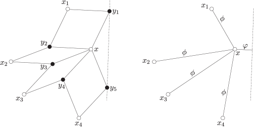
Figure 7: Faces adjacent to the vertex $x$ near a boundary (left). Star graph from the white subgraph where the edges carry the functions associated appearing in the Toda-type equation (right).

As in the bulk case, if the graph is bi-partite (see footnote 2) and moreover if the vertices on the boundary are of the same type, one can reproduce the above procedure on the whole graph to get a Toda-type model on a subgraph and with a boundary determined by $\varphi$. The conditions on the graph seem, at first glance, very restricting. Nevertheless, the procedure explained in Section 2.1 provides, starting from any graph, examples satisfying such constraints.

5.2 Boundary conditions for Toda-type systems

In general, it seems that not all the solutions for $q$ found previously can be written as in (15). However, it turns out that for each solution $q(x,y,z;a)$ for which the corresponding function $k(x,y;a)$ depends only on $y$ or the function $q(x,y,z;a)$ factorizes as $f(y,a)g(x,z,a)$, there is a way to obtain $\varphi$ from $\phi$. This is reminiscent, at the three-leg form level, of the simple folding procedure (7) used to obtain $q$ from $Q$. In these cases, the function $k(x,y;a)$ plays the role of the cut-off constraint (or boundary condition) for the Toda-type model in the sense of [20] (see Example 5.3 below for a precise connection).

For the first case where the function $k(x,u;a)=k(u;a)$ does not depend on $x$, using equation (7) in (13) or (14) together with the $D_{4}$-symmetry property for $Q$, one can see that equation (15) with the following function $\varphi$

$$\varphi(y;a)=\phi(y,k(y;a);a,\sigma(a)),$$ (16)

is equivalent to the corresponding boundary equation $q(x,y,z;a)=0$. Therefore, by using the explicit forms of $\phi$ given in [2] associated to each $Q$ of the ABS classification and the results of Tables 1 and 2, we can derive $\varphi$ and hence three-leg forms of the boundary equation in the form (15). In turn, this allows us to define Toda-type systems with a boundary.

Example 5.1.

The trivial solution (8) always corresponds to $\varphi(y;a)=0$ for the additive case or $\varphi(y;a)=1$ for the multiplicative case. This boundary condition may be interpreted as a free boundary for the corresponding Toda-type system.

Example 5.2.

We recall that $\psi(x,u;a)=\frac{a}{x-u}$ and $\phi(x,y;a,b)=\psi(x,y;a-b)$ for ${\rm Q1}_{\delta=0}$. Looking at the fourth solution for ${\rm Q1}_{\delta=0}$ of Table 1, i.e. $\sigma(a)=-a+2\mu$ and $k(x,y;a)=-y$, we obtain $\varphi$ using (16) and the following discrete Toda-type system with a boundary term:

$$\frac{a_{n}-\mu}{x}+\sum_{k=1}^{n-1}\frac{a_{k}-a_{k+1}}{x-x_{k}}=0.$$

For the second case where the function $q(x,y,z;a)$ factorises, the construction is a bit more involved. The equation $q(x,y,z;a)=0$ constrains $x$ and $z$ independently of the values of $y$. Therefore, we get equations involving only the values of the field on the boundary. Let us suppose we solve these constraints on the boundary and denote by $\bar{x}$ the corresponding solution for the field $x$. These values on the boundary play the role of parameters in the function $k(\bar{x},y;a)$ appearing in the boundary conditions. Also, one can see that equation (15) involves the following function $\varphi_{\bar{x}}$

$$\varphi_{\bar{x}}(y;a)=\phi\big{(}y,k(\bar{x},y;a);a,\sigma(a)\big{)},$$

and is equivalent to the corresponding boundary equation $q(\bar{x},y,\bar{z};a)=0$. It also appears in the corresponding Toda-type system with boundary. We now illustrate this case.

Example 5.3.

Let us restrict our general framework to a ${\mathbb{Z}}^{2}$ lattice system: we consider the quad-graph with boundary represented on Fig. 9 with the bulk equations given by ${\rm Q1}_{\delta=0}$ with the label $a$ on the lines $m-n={\rm const}$ and the label $b\neq a$ on the lines $m+n={\rm const}$. The corresponding Toda-type model reads, for $n\geq 2$,

$$\frac{1}{q_{m,n+1}-q_{m,n}}-\frac{1}{q_{m,n}-q_{m,n-1}}=\frac{1}{q_{m+1,n}-q_{m,n}}-\frac{1}{q_{m,n}-q_{m-1,n}},$$ (17)

We use the third solution for $q$ for ${\rm Q1}_{\delta=0}$ in Table 1 to generate the boundary condition on the Toda-type system from the following boundary equation

$$q(\bar{x}_{m},q_{m,1},\bar{x}_{m+1};a)=0\qquad\Leftrightarrow\qquad\bar{x}_{m}+\bar{x}_{m+1}=0,$$

on the quad-graph with boundary. It is obvious that the general solution for the boundary values of the field is $\bar{x}_{m}=(-1)^{m}\bar{x}_{0}$ (for any $\bar{x}_{0}$). Then, following the procedure of folding explained in Section 3.2, we obtain

$$q_{m,0}=k(\bar{x}_{m},q_{m,1};a),$$ (18)

where

$$k(\bar{x}_{m},q_{m,1};a)=\frac{\mu(-1)^{m}\bar{x}_{0}q_{m,1}+(a-\mu)\bar{x}_{0}^{2}}{(a-\mu)q_{m,1}+\mu(-1)^{m}\bar{x}_{0}}.$$

In particular, we recover exactly the results of [20] (equations (13) and (17)) for the model (17) (equation (3) of [20]) with the identifications

$$\bar{x}_{0}\rightarrow\sqrt{\frac{a}{b}},\qquad a\rightarrow b+c\sqrt{\frac{b}{a}}\qquad\text{and}\qquad\mu\rightarrow c\sqrt{\frac{b}{a}},$$ (19)

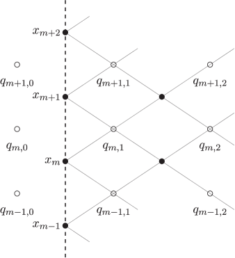
Figure 8: A quad-graph with boundary with an underlying ${\mathbb{Z}}^{2}$ lattice structure. The additional white vertices will play the role of boundary vertices for the Toda-type system with boundary living on the white sublattice.

Figure 9: The (white) ${\mathbb{Z}}^{2}$ (sub)lattice supporting the Toda-type system with a boundary. Our boundary is inserted between the boundary for the Toda-type system at site $n=0$ and the first site of the bulk system at $n=1$.

5.3 Lax presentation of boundary conditions for a Toda-type model

In the previous Example 5.3, we showed that we can recover the boundary conditions introduced in [20]. In this subsection, we show that the correspondence goes beyond this and is in fact also valid at the level of the zero curvature representation. Indeed, our zero curvature representation (11) allows us to recover as a particular case the main equation of [20], which we reproduced as (20) below, and which encodes the symmetry approach to integrable boundary conditions applied to integrable discrete chains. For clarity, we restrict our discussion of this connection to the case treated already in Example 5.3 above. But we believe that the argument is easily generalizable to most Toda-type models.

Let us first recall that the boundary condition (18) was obtained in [20] by analysing the matrix equation

$$H(m+1,\lambda)A(m,0,\lambda)=A(m,0,h(\lambda))H(m,\lambda),$$ (20)

where $A(m,n,\lambda)$ is the “discrete time” part of the discrete Lax pair (evaluated at the site $n=0$ of the boundary), $h$ is some function acting on the parameter $\lambda$ and $H(m,\lambda)$ is a matrix encoding an extra linear symmetry at the site of the boundary (see equations (14) and (15) in [20]) and effectively producing allowed integrable boundary conditions.

The main result here is that our zero curvature representation boils down to (20) thanks to a remarkable “fusion” property of the two matrices $L$ which then become $A$ and the fact that our matrix $K$ becomes the matrix $H$. This goes as follows. The zero curvature representation based on Fig. 9 reads

$$K(x_{m+1};c)L(x_{m+1},q_{m,1},\sigma(a);c)L(q_{m,1},x_{m},a;c)$$

$$\qquad=L(x_{m+1},q_{m,1},\sigma(a);\sigma(c))L(q_{m,1},x_{m},a;\sigma(c))K(x_{m};c),$$

where

$$L(y,x,a;b)=\frac{1}{(x-y)}\left(\begin{matrix}ay+b(x-y)&-axy\\ a&-ax+b(x-y)\end{matrix}\right),$$

and

$$K(x;c)=\left(\begin{matrix}\mu x&(c-\mu)x^{2}\\ (c-\mu)&\mu x\end{matrix}\right).$$

Now, using the three-leg form

$$\psi(q_{m,1},x_{m+1};\sigma(a))-\psi(q_{m,1},x_{m};a)=\phi(q_{m,1},q_{m,0};\sigma(a),a),$$

and performing calculations similar to those in [11, Proposition 11], one finds

$$L(x_{m+1},q_{m,1},\sigma(a);c)L(q_{m,1},x_{m},a;c)=cL(q_{m,0},q_{m,1},\sigma(a)-a;c-a).$$

It remains to perform the changes of parameters as in (19), together with

$$c\rightarrow(2\lambda+1)b+c\sqrt{\frac{b}{a}},$$ (21)

to obtain

$$L(x_{m+1},q_{m,1},\sigma(a);c)L(q_{m,1},x_{m},a;c)=2b\left((2\lambda+1)b+c\sqrt{\frac{b}{a}}\right)\sigma_{3}A(m,n,\lambda)\sigma_{3},$$

where $\sigma_{3}$ is the usual $2\times 2$ Pauli matrix. This also yields

$$K(x_{m};c)=\left(\begin{matrix}(-1)^{m}c&(2\lambda+1)a\\ (2\lambda+1)b&(-1)^{m}c\end{matrix}\right)=(-1)^{m}H(m,\lambda).$$

This is completely equivalent to the results obtained in [20] up to an irrelevant $c\to 1/c$ substitution in $H$. Note that the map $\lambda\mapsto h(\lambda)=-\lambda-1$ is also correctly reproduced with our choice $\sigma(c)=-c+2\mu$ and under the identifications (19) and (21).

6 Connection between 3D boundary consistency
and the set-theoretical reflection equation

6.1 General approach

In [28], a nice approach was described to obtain a relation between a 3D consistent quad-graph equation and a Yang–Baxter map thus yielding a connection between 3D consistency and the set-theoretical Yang–Baxter equation [17]. It is based on the use of symmetries of the equation $Q=0$ and the identification of invariants under these symmetries. Our idea is to extend this connection at the level of reflection maps and integrable boundary equations thus yielding a connection between the 3D boundary consistency introduced here and the set-theoretical reflection equation introduced in [14, 15]. First, let us recall the method of [28]. Given a quad-graph equation

$$Q(u_{00},u_{10},u_{01},u_{11};a,b)=0,$$ (22)

let $G$ be a connected one-parameter group of transformations acting on the variables $u_{ij}$

$$G_{\epsilon}:\ (u_{00},u_{10},u_{01},u_{11})\mapsto(\hat{u}_{00},\hat{u}_{10},\hat{u}_{01},\hat{u}_{11}).$$

This transformation is said to be a symmetry of (22), if

$$Q(\hat{u}_{00},\hat{u}_{10},\hat{u}_{01},\hat{u}_{11};a,b)=0,$$

whenever (22) holds. The corresponding infinitesimal action reads

$$\mathbf{v}Q=0,$$

where

$$\mathbf{v}=\eta_{00}\frac{\partial}{\partial u_{00}}+\eta_{10}\frac{\partial}{\partial u_{10}}+\eta_{01}\frac{\partial}{\partial u_{01}}+\eta_{11}\frac{\partial}{\partial u_{11}},$$

with $\eta$ being the characteristic of $G$ specified by

$$\eta_{ij}=\frac{d}{d\epsilon}G_{\epsilon}(u_{ij}).$$

Methods to obtain the characteristic $\eta$ can be seen, e.g. in [22, 23]. Knowing $\mathbf{v}$, the idea is then to define a lattice invariant $I$ of the transformation group $G$ which satisfies

$$\mathbf{v}I=0,$$

and to use it to define the Yang–Baxter (or edge) variables $(X,Y,U,V)$ from the vertex variables $(u_{00},u_{10},u_{01},u_{11})$ by

$$X=I(u_{00},u_{10}),\qquad Y=I(u_{10},u_{11}),\qquad U=I(u_{01},u_{11}),\qquad V=I(u_{00},u_{01}),$$

and assign them to the edges of an elementary quadrilateral as shown in Fig. 10.

Figure 10: Link between quad-graph equation and Yang–Baxter map.

Once the infinitesimal generator $\mathbf{v}$ is known, one can solve for $I$.

An important result of [28] is that the variables $X$, $Y$, $U$, $V$ are related by a map $(U,V)=R(X,Y)$ which is a Yang–Baxter map, provided the quad-graph equation determined by $Q$ satisfies the 3D-consistency property. To construct boundary equations that satisfy the 3D-boundary consistency property, we propose to use this method “backwards” in connection with our classification of reflection maps associated to quadrirational Yang–Baxter maps. Choosing the invariant properly, the Yang–Baxter map $R$ can be recognized as one canonical form belonging to the classification of quadrirational Yang–Baxter maps [3, 27]. Then we can use the corresponding reflection maps $h_{a}$ and $\sigma$ to construct $q$ according to the following prescription

$$q(u_{10},u_{00},u_{01};a)=I(u_{00},u_{01})-h_{a}(I(u_{00},u_{10})).$$ (23)

The origin of this prescription comes from the folding method explained and used in [14] to construct reflection maps. When translated in terms of vertex variables $u_{00}$, $u_{10}$, $u_{01}$, it gives (23). Indeed, the folding method produces reflection maps $B$ acting on the Yang–Baxter variables and the parameters, of the form $(V,b)=B(X,a)=(h_{a}(X),\sigma(a))$. Hence, $V=h_{a}(X)$ and recalling that $V=I(u_{00},u_{01})$ and $X=I(u_{00},u_{10})$, this becomes equivalent to $q(u_{10},u_{00},u_{01};a)=0$ with $q$ as defined in (23). In particular, our construction ensures that $q$ and $Q$ satisfy the 3D-boundary consistency property since the corresponding Yang–Baxter and reflection maps satisfy the set-theoretical reflection equation. We see that to carry out this programme, the knowledge of the invariants and hence $\mathbf{v}$ is crucial. We use the classification for $\mathbf{v}$ obtained in [29] of the so-called five-point symmetries, a subset of which is the set of one-point symmetries which are the ones involved in the above method. Note that although the results of [29] were obtained in the context of ${\mathbb{Z}}^{2}$ lattices, we can easily adapt them to the present more general context of quad-graphs. For each $\mathbf{v}$ of each quad-graph equation, we provide a solution $I_{0}$ for the invariant $I$ which is of the simplest form, the latter meaning that other solutions are obtained from our $I_{0}$ in the form $f(I_{0})$ with $f$ being a differentiable bijection depending possibly on the parameters $a$ or $b$. To the best of our knowledge, only sparse examples of invariants and corresponding YB maps have been given in the literature so far. In Table 3 below, we give a list of invariants satisfying the above criteria and the corresponding family of YB maps. Then, one only has to use formula (23) to find $q$. In Tables 1 and 2, the solutions for $q$ (and $\sigma$) that we have found using this method (on top of the folding method) are shown with an asterisk.

6.2 Example for $\boldsymbol{{\rm A1}_{\delta=0}}$

We now carry out the example of the quad-graph equation $A1_{\delta=0}$ explicitly to show how the method works and illustrate some of the technical subtleties. Let

$$Q(u_{00},u_{10},u_{01},u_{11},a,b)=a(u_{00}+u_{01})(u_{10}+u_{11})-b(u_{00}+u_{10})(u_{01}+u_{11}).$$

For this family, the classification in [29] gives three one-point symmetry generators

$$\eta_{1}=(-1)^{k+l},\qquad\eta_{2}=u_{00},\qquad\eta_{3}=(-1)^{k+l}u^{2}_{00}.$$

The corresponding simplest invariants $I_{1}$, $I_{2}$ and $I_{3}$ read

$$I_{1}(s,t)=s+t,\qquad I_{2}(s,t)=\frac{s}{t},\qquad I_{3}(s,t)=\frac{1}{s}+\frac{1}{t}.$$

So, for the first invariant, the Yang–Baxter variables read

$$X=u_{00}+u_{10},\qquad Y=u_{10}+u_{11},\qquad U=u_{01}+u_{11},\qquad V=u_{00}+u_{01},$$

which satisfy

$$X-Y=V-U,\qquad aVY-bXU=0.$$ (24)

This yields the relations

$$U=aY\frac{X-Y}{bX-aY},\qquad V=bX\frac{X-Y}{bX-aY}.$$

To recognize the family to which this map belongs, we perform the following transformation on the variables

$$X\to aX,\qquad Y\to bY,\qquad U\to aU,\qquad V\to bV.$$ (25)

We then obtain the $F_{\rm III}$ quadrirational Yang–Baxter map

$$U=\frac{Y}{a}P,\qquad V=\frac{X}{b}P,\qquad P=\frac{aX-bY}{X-Y}.$$

For this family, we have the following reflections maps

$$\sigma(a)=\frac{\mu^{2}}{a}\qquad\text{and}\qquad h_{a}(X)=\frac{aX}{\mu}\qquad\text{or}\qquad h_{a}(X)=-\frac{aX}{\mu},$$

where $\mu$ is a free parameter. Performing the inverse transformation of (25), we obtain the reflection maps that we can use in formula (23) to obtain $q$. They read

$$h_{a}(X)=\frac{\mu X}{a}\qquad\text{or}\qquad h_{a}(X)=-\frac{\mu X}{a},$$

and we obtain

$$q(x,y,z;a)=\mu(x+y)-a(y+z)\qquad\text{or}\qquad q(x,y,z;a)=\mu(x+y)+a(y+z),$$

both valid with $\sigma(a)=\frac{\mu^{2}}{a}$. Note that in this case, the two possibilities for the boundary equations $q(u_{10},u_{00},u_{01};a)=0$ are related by the transformation $\mu\to-\mu$ which leaves $\sigma(a)$ invariant so that, in fact, we only have one boundary equation here.

Let us perform the same analysis for $I_{2}$. The Yang–Baxter variables are

$$X=u_{00}/u_{10},\qquad Y=u_{10}/u_{11},\qquad U=u_{01}/u_{11},\qquad V=u_{00}/u_{01},$$

and they satisfy

$$XY=UV,\qquad a(XY+U)(Y+1)-bY(X+1)(U+1)=0,$$

which yields

$$U=\frac{bY-aXY+bXY-aXY^{2}}{a+aY-bY-bXY},\qquad V=\frac{aX+aXY-bXY-bX^{2}Y}{b-aX+bX-aXY}.$$

Performing the following transformation

$$X\to-X,\qquad Y\to-Y,\qquad U\to-U,\qquad V\to-V,$$ (26)

we obtain the $H_{\rm II}$ quadrirational Yang–Baxter map

$$U=Y\frac{(b+(a-b)X-aXY)}{(a+(b-a)Y-bXY)},\qquad V=X\frac{(a+(b-a)Y-bXY)}{(b+(a-b)X-aXY)}.$$

For this family, we have the following reflections maps

$$\sigma(a)=\frac{\mu^{2}}{a}\qquad\text{and}\qquad h_{a}(X)=\frac{a+\mu-X\mu}{a}\qquad\text{or}\qquad h_{a}(X)=\frac{aX}{aX+\mu-X\mu},$$

or,

$$\sigma(a)=-a+2\mu\qquad\text{and}\qquad h_{a}(X)=-X\qquad\text{or}\qquad h_{a}(X)=\frac{a+(X-1)\mu}{aX+\mu-X\mu}.$$

where $\mu$ is a free parameter. Performing the inverse transformation of (26) and using (23) we find

$$q(x,y,z;a)=ax(y+z)+(x+y)z\mu\qquad\text{or}\qquad q(x,y,z;a)=y(a(y+z)-(x+y)\mu),$$

both valid with $\sigma(a)=\frac{\mu^{2}}{a}$, and,

$$q(x,y,z;a)=y(x+z)\qquad\text{or}\qquad q(x,y,z;a)=a\left(y^{2}-xz\right)-(x+y)(y-z)\mu,$$

both valid for $\sigma(a)=-a+2\mu$.

Finally, using $I_{3}$ yields the relations (24) so that we obtain the $F_{\rm III}$ quadrirational Yang–Baxter map again. Therefore, we can use the same reflection maps but because the invariant is different we may obtain different expressions for $q$. A direct calculation gives

$$q(x,y,z;a)=ax(y+z)+(x+y)z\mu\qquad\text{or}\qquad q(x,y,z;a)=ax(y+z)-(x+y)z\mu,$$

both valid with $\sigma(a)=\frac{\mu^{2}}{a}$. These are in fact the same solution under the transformation $\mu\to-\mu$ and it coincides with the first solution already obtained from the $H_{\rm II}$ family. Let us remark that in some cases, point transformations on the parameters are needed on top of Möbius transformations to recognize the canonical Yang–Baxter map. This may affect the form of the map $\sigma$ to be used in the 3D boundary consistency condition. This happens for ${\rm Q3}_{\delta=0}$, $\rm H3$ and $\rm A2$. Finally, let us also mention that this method has some inherent limitations due to the fact that for families ${\rm Q2}$, ${\rm Q3}_{\delta=1}$ and $\rm Q4$, there are no one-point symmetry generators in the classification of [29]. Our other method described in Section 3 does also work for these families, as can be seen in the tables. Whether or not the corresponding solutions for $q$ for these “missing” families can be mapped back to reflection maps is an interesting open question.

Table 3: Some invariants and corresponding Yang–Baxter maps for the ABS quad-graph equations.

Quad-graph equation	Characteristic	Invariant	Yang–Baxter map2pt2pt
Q1δ=0	$\eta_{1}=1$	$I(s,t)=s-t$	$H_{{\rm III}a}$2pt2pt
	$\eta_{2}=u_{00}$	$I(s,t)=s/t$	$H_{\rm II}$2pt
	$\eta_{3}=u^{2}_{00}$	$I(s,t)=1/s-1/t$	$H_{{\rm III}a}$2pt
Q1δ=1	$\eta_{1}=1$	$I(s,t)=s-t$	$H_{\rm II}$2pt2pt
Q3δ=0	$\eta_{1}=u_{00}$	$I(s,t)=s/t$	$H_{\rm I}$2pt2pt
H1	$\eta_{1}=1$	$I(s,t)=s-t$	$H_{\rm V}$2pt2pt
	$\eta_{2}=(-1)^{k+l}$	$I(s,t)=s+t$	$F_{\rm V}$2pt
	$\eta_{3}=(-1)^{k+l}u_{00}$	$I(s,t)=st$	$F_{\rm IV}$2pt
H2	$\eta_{1}=(-1)^{k+l}$	$I(s,t)=s+t$	$F_{\rm IV}$2pt2pt
H3δ=0	$\eta_{1}=u_{00}$	$I(s,t)=s/t$	$H_{{\rm III}b}$2pt2pt
	$\eta_{2}=(-1)^{k+l}u_{00}$	$I(s,t)=st$	$F_{\rm III}$2pt
H3δ=1	$\eta_{1}=(-1)^{k+l}u_{00}$	$I(s,t)=st$	$F_{\rm II}$2pt2pt
A1δ=0	$\eta_{1}=(-1)^{k+l}$	$I(s,t)=s+t$	$F_{\rm III}$2pt2pt
	$\eta_{2}=u_{00}$	$I(s,t)=s/t$	$H_{\rm II}$2pt
	$\eta_{3}=(-1)^{k+l}u^{2}_{00}$	$I(s,t)=1/s+1/t$	$F_{\rm III}$2pt
A1δ=1	$\eta_{1}=(-1)^{k+l}$	$I(s,t)=s+t$	$F_{\rm II}$2pt2pt
A2	$\eta_{1}=(-1)^{k+l}u_{00}$	$I(s,t)=st$	$F_{\rm I}$2pt2pt

7 Conclusions and outlooks

We proposed a definition for integrable equations on a quad-graph with boundary and introduced the notion of 3D boundary consistency as a complement of the 3D consistency condition that is used as an integrability criterion for bulk quad-graph systems. Just like quadrilaterals are fundamental structures when one discretizes an arbitrary surface without boundary, we argued that triangles appear naturally when one considers surfaces with boundary. Therefore, it is natural to associate a $3$-point boundary equation to describe the boundary locally just like one associates a $4$-point bulk equation to describe the bulk locally. We presented two different methods to find solutions of the 3D boundary consistency condition given an integrable quad-graph equation of the ABS classification. The terminology “integrable boundary” is also backed up by the discussion of other traditional integrable structures like Bäcklund transformations and zero curvature representation for systems with boundary. This is also supported by the connection that we unraveled between 3D boundary consistency and set-theoretical reflection equation. As a by-product of our study, we were also able to introduce three-leg forms of boundary equations and hence to introduce Toda-type systems with boundary.

The present work lays some foundations for what we hope could be a new exciting area of research in discrete integrable systems. Among the many open questions one can think of, we would like to mention a few that we believe are important: finding a method of classification of boundary equations given a bulk quad-graph equation, tackling the problem of posing the initial-boundary value problem for quad-graph equations with a boundary, understanding the connection of our approach with the singular-boundary reduction approach of [6], implementing the discrete inverse scattering method with a boundary with the hope of finding soliton solutions, etc.

Acknowledgements

The final details of this paper were completed while two of the authors (V.C. and Q.C.Z) were at the “Discrete Integrable Systems” conference held at the Newton Institute for Mathematical Sciences. We wish to thank C. Viallet for pointing out useful references. We also thank M. Nieszporski and P. Kassotakis for useful discussions and the provision of unpublished material on their work on the connection between Yang–Baxter maps and quad-graph equations, some of which is related to our results shown in Table 3. Last, but not least, we express our sincere gratitude to the referees whose excellent comments and criticisms helped improve this paper tremendously.

References

- [1] Adler V.E., Discrete equations on planar graphs, J. Phys. A: Math. Gen. 34 (2001), 10453–10460.
- [2] Adler V.E., Bobenko A.I., Suris Yu.B., Classification of integrable equations on quad-graphs. The consistency approach, Comm. Math. Phys. 233 (2003), 513–543, nlin.SI/0202024.
- [3] Adler V.E., Bobenko A.I., Suris Yu.B., Geometry of Yang–Baxter maps: pencils of conics and quadrirational mappings, Comm. Anal. Geom. 12 (2004), 967–1007, math.QA/0307009.
- [4] Ahn C., Koo W.M., Boundary Yang–Baxter in the RSOS/SOS representation, in Statistical Models, Yang–Baxter Equation and Related Topics, and Symmetry, Statistical Mechanical Models and Applications (Tianjin, 1995), World Sci. Publ., River Edge, NJ, 1996, 3–12, hep-th/9508080.
- [5] Atkinson J., Hietarinta J., Nijhoff F., Seed and soliton solutions for Adler’s lattice equation, J. Phys. A: Math. Theor. 40 (2007), F1–F8, nlin.SI/0609044.
- [6] Atkinson J., Joshi N., Singular-boundary reductions of type-Q ABS equations, Int. Math. Res. Not. 2013 (2013), 1451–1481, arXiv:1108.4502.
- [7] Baxter R.J., The Yang–Baxter equations and the Zamolodchikov model, Phys. D 18 (1986), 321–347.
- [8] Bazhanov V.V., Mangazeev V.V., Sergeev S.M., Quantum geometry of three-dimensional lattices, J. Stat. Mech. Theory Exp. 2008 (2008), P07004, 27 pages, arXiv:0801.0129.
- [9] Behrend R.E., Pearce P.A., O’Brien D.L., Interaction-round-a-face models with fixed boundary conditions: the ABF fusion hierarchy, J. Statist. Phys. 84 (1996), 1–48, hep-th/9507118.
- [10] Bellon M.P., Viallet C.-M., Algebraic entropy, Comm. Math. Phys. 204 (1999), 425–437, chao-dyn/9805006.
- [11] Bobenko A.I., Suris Yu.B., Integrable systems on quad-graphs, Int. Math. Res. Not. 2002 (2002), 573–611, nlin.SI/0110004.
- [12] Bobenko A.I., Suris Yu.B., Discrete differential geometry. Integrable structure, Graduate Studies in Mathematics, Vol. 98, American Mathematical Society, Providence, RI, 2008, math.DG/0504358.
- [13] Boll R., Classification of 3D consistent quad-equations, J. Nonlinear Math. Phys. 18 (2011), 337–365, arXiv:1009.4007.
- [14] Caudrelier V., Crampé N., Zhang Q.C., Set-theoretical reflection equation: classification of reflection maps, J. Phys. A: Math. Theor. 46 (2013), 095203, 12 pages, arXiv:1210.5107.
- [15] Caudrelier V., Zhang Q.C., Yang–Baxter and reflection maps from vector solitons with a boundary, arXiv:1205.1133.
- [16] Cherednik I.V., Factorizing particles on a half-line and root systems, Theoret. and Math. Phys. 61 (1984), 977–983.
- [17] Drinfeld V.G., On some unsolved problems in quantum group theory, in Quantum Groups (Leningrad, 1990), Lecture Notes in Math., Vol. 1510, Springer, Berlin, 1992, 1–8.
- [18] Fan H., Hou B.Y., Shi K.J., General solution of reflection equation for eight-vertex SOS model, J. Phys. A: Math. Gen. 28 (1995), 4743–4749.
- [19] Grammaticos B., Ramani A., Papageorgiou V., Do integrable mappings have the Painlevé property?, Phys. Rev. Lett. 67 (1991), 1825–1828.
- [20] Habibullin I.T., Kazakova T.G., Boundary conditions for integrable discrete chains, J. Phys. A: Math. Gen. 34 (2001), 10369–10376.
- [21] Hietarinta J., Searching for CAC-maps, J. Nonlinear Math. Phys. 12 (2005), suppl. 2, 223–230.
- [22] Levi D., Petrera M., Scimiterna C., The lattice Schwarzian KdV equation and its symmetries, J. Phys. A: Math. Theor. 40 (2007), 12753–12761, math-ph/0701044.
- [23] Levi D., Winternitz P., Continuous symmetries of difference equations, J. Phys. A: Math. Gen. 39 (2006), R1–R63, nlin.SI/0502004.
- [24] Mercat C., Holomorphie discrète et modèle d’Ising, Ph.D. Thesis, Université Louis Pasteur, Strasbourg, France, 1998, available at http://tel.archives-ouvertes.fr/tel-00001851/.
- [25] Mercat C., Discrete Riemann surfaces and the Ising model, Comm. Math. Phys. 218 (2001), 177–216.
- [26] Nijhoff F.W., Lax pair for the Adler (lattice Krichever–Novikov) system, Phys. Lett. A 297 (2002), 49–58, nlin.SI/0110027.
- [27] Papageorgiou V.G., Suris Yu.B., Tongas A.G., Veselov A.P., On quadrirational Yang–Baxter maps, SIGMA 6 (2010), 033, 9 pages, arXiv:0911.2895.
- [28] Papageorgiou V.G., Tongas A.G., Veselov A.P., Yang–Baxter maps and symmetries of integrable equations on quad-graphs, J. Math. Phys. 47 (2006), 083502, 16 pages, math.QA/0605206.
- [29] Rasin O.G., Hydon P.E., Symmetries of integrable difference equations on the quad-graph, Stud. Appl. Math. 119 (2007), 253–269.
- [30] Sklyanin E.K., Boundary conditions for integrable quantum systems, J. Phys. A: Math. Gen. 21 (1988), 2375–2389.