Exact and approximate expansions with pure Gaussian wavepackets

Abstract.

We construct frames of wavepackets produced by parabolic dilation, rotation and translation of (a finite sum of) Gaussians and give asymptotics on the analogue of Daubechies frame criterion. We show that the coefficients in the corresponding approximate expansion decay fast away from the wavefront set of the original data.

1. Introduction

Wavepackets are a powerful tool for the microlocal analysis of (Fourier integral) operators and their wave front sets [13, 38, 39]. A “second dyadic decomposition” [40] with parabolic scaling and rotations endows them with the necessary directional sensitivity to resolve singularities. Related objects, such as curvelets and shearlets, incorporate similar features, in particular the parabolic dilations. Frames of these also facilitate methods to sparsify Fourier integral operators and resolve the wavefront set; the emphasis is often on the applications to image processing and numerical aspects. See [10, 11, 23, 32, 6] for representative references.

We consider wavepackets produced by parabolic dilation, rotation and translation of a function $\varphi:{\mathbb{R}^{2}}\to{\mathbb{C}}$, given by

(1) $$\varphi_{j,k,\lambda}(x):=8^{j/2}\varphi(A_{j,k}x-\lambda),\qquad(j\geq 1,0\leq k\leq 2^{j}-1,\lambda\in\Lambda),$$

where

$$A_{j,k}:=\begin{bmatrix}4^{j}&0\\ 0&2^{j}\end{bmatrix}\begin{bmatrix}\cos(\frac{2k\pi}{2^{j}})&-\sin(\frac{2k\pi}{2^{j}})\\ \sin(\frac{2k\pi}{2^{j}})&\cos(\frac{2k\pi}{2^{j}})\end{bmatrix},$$

and $\Lambda\subseteq{\mathbb{R}^{2}}$ is a lattice. If $\varphi$ is rapidly decaying, the packet $\varphi_{j,k,\lambda}$ is localized near $A_{j,k}^{-1}\lambda$ and aligned to an angle of $\frac{-2\pi k}{2^{j}}$ radians. For the coarse scales we use translates of a second window ${\varphi_{0,\lambda}}:={\varphi_{0}}(\cdot-\lambda)$, which typically is a symmetric Gaussian centered at 0. The complete collection of such wavepackets is then the set

(2) $$\mathcal{C}_{\Lambda}:=\big{\{}\,{\varphi_{0,\lambda}}\,\big{|}\,\lambda\in\Lambda\,\big{\}}\cup\big{\{}\,\varphi_{j,k,\lambda}\,\big{|}\,\lambda\in\Lambda,j\geq 1,0\leq k\leq 2^{j}-1\,\big{\}}.$$

Our contribution is twofold: First we consider exact expansions and approximate expansions of $L^{2}(\mathbb{R}^{2})$ functions in terms of these packets using Gaussian windows. Second we study the wavefront set with respect to a frame of wavepackets.

The motivation for using purely Gaussian windows comes from highly efficient numerical algorithms [4], with applications in reflection and global seismology. The Gaussian is the window of choice, because it has the best localization in phase-space and yields the best resolution. The use of wavepackets that consist of pure Gaussians has several technical advantages because a number of computations can be done explicitly.

Applications include data compression, denoising, and wavefield recovery from finite data [2, 3, 41], and wave propagation and inverse scattering described by Fourier integral operators associated with canonical graphs. For the latter application, see [17]. Purely Gaussian wave packets are effective in the parametrix construction of the wave equation. Here the the initial data are decomposed with respect to a frame of such wave packets, because a Gaussian wave packet naturally matches the initial conditions for a multi-scale Gaussian-beam-like solution [35]. Gaussian beams are designed to account for the formation of caustics. The frame property facilitates the derivation of error estimates for the parametrix which decay under scale refinement. One can also generate multi-scale Gaussian-beam-like solutions from the decomposition of boundary values, which play a role in the development of inverse scattering algorithms via wavefield cross correlation that are based on efficient reverse-time continuation [33].

We refer the reader to [4] for a comparison of curvelets and Gaussian wavepackets and  [7] for the use of Gaussians as wavelets for the continuous wavelet transform. Whereas the recent results on curvelets and shearlets emphasize the construction of tight frames with compactly supported windows or bandlimited windows [1, 12, 23, 14, 36, 30, 28], we understand much less about the spanning properties and the frame properties of wavepackets with Gaussian windows. For instance, Andersson, Carlsson, and Tenorio  [4] treat the effective approximation of bounded compactly-supported functions by this kind of packets, but they left open the question whether a full expansion by a set $\mathcal{C}_{\Lambda}$ of Gaussian wavepackets represents every function in $L^{2}(\mathbb{R}^{2})$. Likewise, most of the work on Gaussian beams [3, 34, 35, 37] emphasizes the algorithmic aspects and contents itself with good numerical approximations. The question of exact representations by a wavepacket expansion is omitted.

Our work complements the numerical results in [4, 35]. We will show in Theorem 3.3 that the wavepacket system $\mathcal{C}_{\Lambda}$ constitutes a frame for a large class of Gaussian-like windows and suitable lattices $\Lambda$.

Using a Gaussian window adds numerous (technical) difficulties to the rigorous analysis of wavepacket expansions. On the one hand, the Gaussian does not have vanishing moments, which is an absolute must in this analysis. On the other hand, the Gaussian is neither compactly supported nor bandlimited; this requires delicate estimates to control the overlap of dilates and rotations of the Gaussian (see Proposition 2.3).

The problems due to the lack of vanishing moments can be circumvented, as with Morlet’s wavelets, by considering linear combinations of modulated Gaussians. As a fundamental example we consider windows of the form,

(3) $$\widehat{\varphi}(\xi_{1},\xi_{2}):=\sum_{k=1}^{N}a_{k}e^{-\left(\delta_{0}\left|\xi_{1}-t_{k}\right|^{2}+\delta_{k}\left|\xi_{2}\right|^{2}\right)},\qquad\xi=(\xi_{1},\xi_{2})\in{\mathbb{R}^{2}},$$

where the points $t_{1},\ldots,t_{N}$, the dilation parameters $\delta_{0},\ldots,\delta_{N}$ and the coefficients $a_{1},\ldots,a_{N}$ are chosen so that

(4) $$\widehat{\varphi}(0)=\partial_{\xi_{1}}\widehat{\varphi}(0)=\ldots=\partial^{N}_{\xi_{1}}\widehat{\varphi}(0)=0.$$

For such a choice of $\varphi$, the wavepackets in (1) are finite linear combinations of Gaussians with different eccentricities, scales and centers. It should be noted that this is different from other Gaussian wavepackets that enforce the vanishing moments through a scale-dependent frequency cut-off (see for example [5]).

The formula in (3) allows for a number of rather different windows. One possibility is to let $\widehat{\varphi(\xi)}$ be essentially a translated Gaussian $e^{-\left|\xi-(0,t_{1})\right|^{2}}$, where $t_{1}>>0$. This window is then corrected with other Gaussians centered near the origin, so as to obtain several vanishing moments. If $t_{1}>>0$, the coefficients corresponding to these correcting terms can be numerically neglected. The case where $t_{1}$ is not large enough to make the correcting terms negligible is also of practical interest. In this case the window $\varphi$ does not look like a pure Gaussian (see Figure 1). Nevertheless, an expansion in terms of the packets in (3) leads to an expansion in terms of Gaussians.

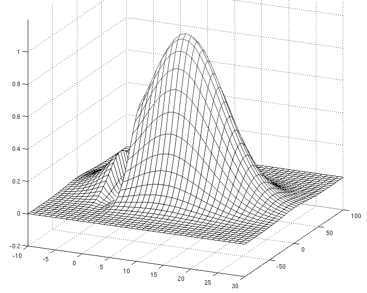
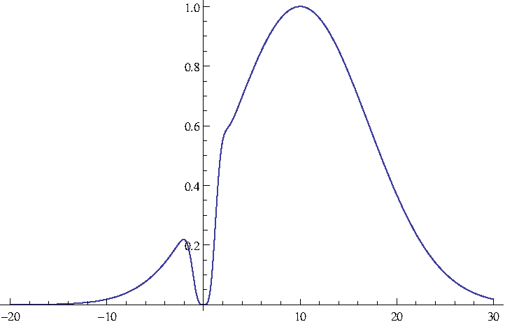
Figure 1. A possible choice of $\widehat{\varphi}$ with vanishing moments of order 3. On the left, a plot of $\widehat{\varphi}$, and on the right a plot of its restriction to the $\xi_{1}$ axis.

$$\widehat{\varphi(\xi)}=g_{1}(\xi_{1})g_{2}(\xi_{2})$$

$$g_{1}(t)\approx e^{-\frac{(t-10)^{2}}{100}}+0.578e^{-(t-1)^{2}}-3.45205e^{-(t-0.5)^{2}}+4.66167e^{-(t-0.25)^{2}}-2.27129e^{-t^{2}}$$

$$g_{2}(t)=e^{-\frac{t^{2}}{1100}}.$$

Throughout the article we make the following assumptions on the windows ${\varphi_{0}},\varphi\in L^{2}({\mathbb{R}^{2}})$.

(5) $$0<A\leq\left|\widehat{{\varphi_{0}}}(\xi)\right|^{2}+\sum_{j\geq 1}\sum_{k=0}^{2^{j}-1}\left|\widehat{\varphi}(B_{j,k}\xi)\right|^{2}\leq B<+\infty,\mbox{ where }B_{j,k}:=(A^{*}_{j,k})^{-1},$$

(6) $$\left|\widehat{{\varphi_{0}}}(\xi)\right|\lesssim e^{-\delta\left|\xi\right|^{2}},$$

(7) $$\left|\widehat{\varphi}(\xi)\right|\lesssim\min(1,\left|\xi_{1}\right|^{{\varsigma}})e^{-\delta\left|\xi\right|^{2}},\mbox{ for some }\delta>0\mbox{ and }{\varsigma}>2.$$

The assumption in (5) means that the windows are wide enough so as to cover the whole frequency plane (see figure 2). The Gaussian wavepackets in (3) clearly satisfy the decay conditions in (6) and (7) while the vanishing moments in the direction $\xi_{1}$ are granted by (4).

Our main result shows that $\mathcal{C}_{\Lambda}$ is a frame for $L^{2}(\mathbb{R}^{2})$ for sufficiently fine lattices $\Lambda$. In Theorem 3.6 we give asymptotics on the lattice parameters required for these packets to generate a frame. The proof uses the method that was developed by Daubechies for wavelets [15]. We will examine the quantities that appear in (the analogue of) Daubechies’ criterion for wavelets, and then bound the correlation between rotations and dilations of the window. A similar approach (involving fewer technicalities) was recently carried out in [28] for the so-called cone-adapted shearlets, in order to obtain compactly supported atoms. The fact that Daubechies’ criterion can be satisfied at all proves that every $L^{2}(\mathbb{R}^{2})$ function can be expanded in terms of pure Gaussian packets. Thus our main result provides theoretical support for the accuracy of numerical wavepacket methods in [4].

As a by-product of using Daubechies’ criterion, we obtain a simple approximate dual frame of the wavepacket system $\mathcal{C}_{\Lambda}$. The main term of the associated frame operator can be written as a Fourier multiplier. Applying the inverse of this Fourier multiplier to the wavepackets we obtain an approximate dual frame that can be easily computed with a simple frequency filter. The error estimate given in Theorem 3.12 may be used to justify when to use the simple approximate expansion (without knowledge of a precise dual frame). In the applications to geophysics that motivated us, the data are noisy and possess a limited numerical accuracy [18]. Therefore, the explicit, simple, but only approximate expansion of the wavefield will be sufficient for many purposes in this context.

Our second contribution is the investigation of the wavefront set with Gaussian wavepackets. We will study the behavior of the coefficients $\left<f,\varphi_{j,k,\lambda}\right>$ as $j\rightarrow+\infty$. Since $\mathcal{C}_{\Lambda}$ is parametrized by a discrete set and is not invariant under translations and rotations, we need to select the parameters $k=k_{j},\lambda=\lambda_{j}$ as a function of the scale in order to track a given phase-space point. Thus the discrete description is more subtle than the descriptions with a continuous transform in [19, 11, 21, 29, 25]. In Theorem 4.1 we will show that if a point does not belong to the wavefront set of $f$ with respect to a Sobolev space $H^{s}$, then the corresponding coefficients decay like $4^{-js}$. We also consider the approximate wavepacket expansion of Section 3.4 and show that the coefficients decay fast in the scale parameter $j$, away from the wavefront set of the original data. It is worth pointing out that wavefront sets can be characterized with other types of anisotropies besides the parabolic one, see for example [19, Theorem 3.29]. The parabolic scaling, however, is essential for the efficient representation of functions with singularities along smooth curves.

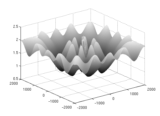
Figure 2. A plot of the quantity in (5) for the function $\varphi$ from Fig. 1 and ${\varphi_{0}}(\xi)=e^{-\frac{\left|\xi\right|^{2}}{10000}}$, showing $A\approx 0.9503$ and $B\approx 2.2483$.

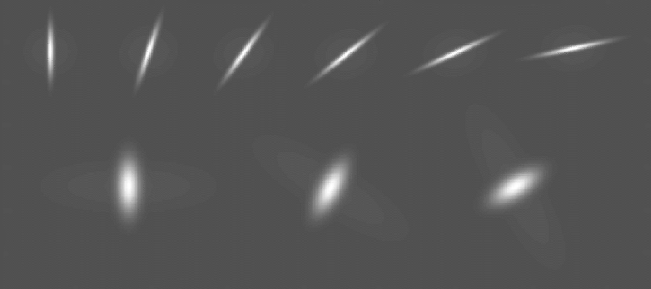
Figure 3. A time-domain display of the wavepackets associated with the window depicted in Figure 1 (absolute value).

1.1. Related work

The Gaussian wavepackets that we treat in this article share the geometric features of other parabolic wavepackets including curvelets and shearlets. Specifically, the atoms are concentrated on elongated regions obeying the relation: width $\approx$ length² and oscillate across their ridge. The packets in (1) are produced exactly by applying a parabolic dilation, rotation and translation to a single window function. In constrast, the classic Gaussian wavepackets from [13, 39, 5] use an additional frequency cut-off to enforce vanishing moments. The curvelets from [10] are produced by parabolic dilation and rotation of a slightly different window at each scale. In the case of shearlets, rotations are replaced by the shear maps $S_{s}(x,y)=(x+sy,y)$. Wave packets based on tilings of frequency space are discussed in  [1, 30, 8, 31].

While the differences between the various parabolic wavepackets are very relevant in practice, their asymptotic properties are similar. The Gaussian wavepackets in (1) are an example of curvelet molecules from [9] and therefore they provide the same sparse approximation properties as curvelets for functions with discontinuities along smooth edges [10]. The notion of curvelet molecules and the related notion of shearlet molecules in [24] are in turn particular cases of the notion of parabolic molecules, as recently introduced in [22]. In that article it is shown that all expansions with adequate systems of parabolic molecules share similar asymptotic properties. As a consequence, our results on the decay of frame coefficients away from the wavefront set can be transferred to other parabolic systems.

Closest to our work is the construction of curvelet-type expansions in [36]. Whereas we construct frames by using an analogue of Daubechies criterion for wavelets, the curvelet-type frames for $L^{2}(\mathbb{R}^{2})$ in [36] are obtained by using a perturbation argument. The main focus of that work is the production of compactly-supported atoms, but the results also apply to sums of modulated Gaussians. As mentioned in [36, Section 6], the perturbation argument yields a frame where each element is a linear combination of dilated, rotated and translated Gaussians. However, the coefficients in that linear combination depend on the indices of the particular frame element, but the number of terms is proved to be uniformly bounded. By contrast, the packets in (1) consist exactly of parabolic dilations, rotations and translations of a single function, which may be taken to be a fixed linear combination of Gaussians.

The Gaussian wavepackets with parabolic scaling in (1) provide an optimal representation of functions with singularities along smooth curves [10], sparsify Fourier wave propagators [9], and are particularly useful in geophysics [18]. For other kinds of applications, other geometries are more adequate. For example, in [16] it is shown that a dictionary of wave-atoms with the scaling “wavelength $\approx$ diameter²” is optimal for the representation of oscillatory patterns (texture).

1.2. Organization

The paper is organized as follows. In Section 2 we derive certain estimates on rotation-dilation overlaps. This is perhaps the main technical contribution when working with Gaussian wavepackets. In Section 3 we develop a Daubechies-like frame criterion and derive conditions for when the wavepacket system $\mathcal{C}_{\Lambda}$ is a frame. We also study the approximate expansions. In Section 4 we study the complement of the wavefront set and describe it by the decay of the coefficients $\left<f,\varphi_{j,k,\lambda}\right>$ as $j\rightarrow+\infty$. Finally we show that similar estimates hold for the coefficients in the approximate expansion related to Daubechies’ criterion.

Notation: In the sequel we use the following notation. We let $1_{E}$ denote the characteristic function of a set $E\subseteq{\mathbb{R}^{2}}$ and $\left|x\right|$ denote the Euclidean norm of a vector $x\in{\mathbb{R}^{2}}$. The Fourier transform is normalized as $\mathcal{F}f(\xi)=\hat{f}(\xi):=\int_{\mathbb{R}^{2}}f(x)e^{-2\pi i\xi x}\,dx$. Translations and dilations of function $f:{\mathbb{R}^{2}}\to{\mathbb{C}}$ are defined as

$$\mathrm{Dil}_{A}f(x):=\left|\det(A)\right|^{1/2}f(Ax),\quad A\in{\mathbb{R}}^{2\times 2},$$

$$T_{y}f(x):=f(x-y).$$

With this notation, $\varphi_{j,k,\lambda}=\mathrm{Dil}_{A_{j,k}}T_{\lambda}\varphi$. Note also that with this notation $\mathrm{Dil}_{A\cdot B}f=\mathrm{Dil}_{B}\mathrm{Dil}_{A}f$.

Let us further denote the parabolic dilations and the rotations by

$$D_{j}=\begin{bmatrix}4^{j}&0\\ 0&2^{j}\end{bmatrix},\qquad R_{\theta}=\begin{bmatrix}\cos(\theta)&-\sin(\theta)\\ \sin(\theta)&\cos(\theta)\end{bmatrix}.$$

Hence $A_{j,k}=D_{j}R_{\frac{2k\pi}{2^{j}}}$ and $B_{j,k}:=(A^{*}_{j,k})^{-1}=D_{j}^{-1}R_{\frac{2k\pi}{2^{j}}}$.

If the lattice $\Lambda$ is given by $\Lambda=P{\mathbb{Z}^{2}}$, with $P\in{\mathbb{R}}^{2\times 2}$ invertible, then we denote its volume by $\left|\Lambda\right|=\left|\det{P}\right|$ and its dual lattice by $\Gamma=(P^{-1})^{*}{\mathbb{Z}^{2}}$.

2. Estimates for rotation-dilation overlaps

We now prove certain technical estimates on rotation-dilation overlaps that will be needed throughout the article. For $f:{\mathbb{R}^{2}}\to{\mathbb{C}}$ let the star-norm of $f$ be defined by

(8) $$\lVert f\rVert_{*}:=\mathop{\operatorname{esssup}}_{\xi\in{\mathbb{R}^{2}}}\sum_{j\geq 1}\sum_{k=0}^{2^{j}-1}\left|f(B_{j,k}\xi)\right|.$$

Let us define the circular sectors,

(11) $$V_{s,t}:=\left\{(r\cos(\theta),r\sin(\theta)):\begin{array}[]{l}2^{s}\leq r\leq 2^{s+1},0\leq\theta\leq\pi/2,\\ 2^{-(t+1)}\leq\cos(\theta)\leq 2^{-t}\end{array}\right\},\quad(s\in{\mathbb{Z}},t\geq 0).$$

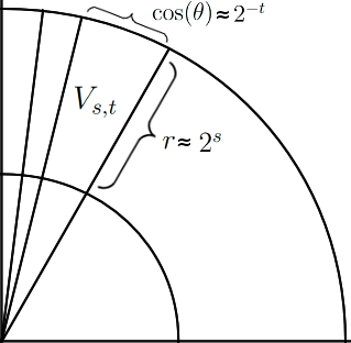
Figure 4. The set $V_{s,t}$ defined in (11).

The next lemma estimates the overlaps of the orbit of each of these sets under parabolic dilations and rotations.

Lemma 2.1.

Let $V_{s,t}$ be defined by (11). Then $\lVert 1_{V_{s,t}}\rVert_{*}\lesssim 4^{t}$.

Proof.

The effect of the parabolic dilation $D_{j}$ can be described (on the first quadrant) in the following way.

(12) $$D_{j}(r\cos(\theta),r\sin(\theta))=(r^{\prime}\cos(\theta^{\prime}),r\sin(\theta^{\prime})),$$

(13) $$r^{\prime}=\rho(\cos(\theta),j)r,$$

(14) $$\tan(\theta^{\prime})=2^{-j}\tan(\theta),$$

where $0\leq\theta\leq\pi/2$, $r>0$, and $\rho(\alpha,j)\geq 0$ is given by

(15) $$\rho(\alpha,j)^{2}=\alpha^{2}4^{2j}+(1-\alpha^{2})2^{2j},\qquad(\alpha\in[0,1],j\in{\mathbb{N}}).$$

We note that $\rho(\alpha,j)$ satisfies the growth estimates,

(16) $$\rho(\alpha,j+1)\geq 2\rho(\alpha,j),$$

(17) $$\rho(\alpha/2,j+2)\geq 2\rho(\alpha,j),\qquad(\alpha\in[0,1],j\in{\mathbb{N}}).$$

Note also that for fixed $j\in{\mathbb{N}}$, $\rho(\alpha,j)$ is increasing in $\alpha$.

With this description, we estimate the image of $V_{s,t}$ under the parabolic dilation $D_{j}$. For $s\in{\mathbb{Z}}$, $t\geq 0$ and $j\in{\mathbb{N}}$, let us define

$$W_{j,s,t}:=\left\{(r\cos(\theta),r\sin(\theta)):\begin{array}[]{c}2^{s}\rho(2^{-(t+1)},j)\leq r\leq 2^{s+1}\rho(2^{-t},j)\\ 0\leq\theta\leq\pi/2\min\{1,2^{-j}4^{t+1}\}\end{array}\right\}.$$

We note that

(18) $$D_{j}V_{s,t}\subseteq W_{j,s,t}.$$

Indeed, if $\xi=(r\cos(\theta),r\sin(\theta))\in V_{s,t}$ and $D_{j}\xi=(r^{\prime}\cos(\theta^{\prime}),r^{\prime}\sin(\theta^{\prime}))$, then by (12),

$$r^{\prime}=\rho(\cos(\theta),j)r\in r[\rho(2^{-(t+1)},j),\rho(2^{-t},j)]\subseteq[2^{s}\rho(2^{-(t+1)},j),2^{s+1}\rho(2^{-t},j)].$$

Since $\xi$ belongs to the first quadrant, so does $D_{j}\xi$. Hence, $\theta^{\prime}\in[0,\pi/2)$. In addition, using (14) and the mean value theorem we estimate,

$$\theta^{\prime}\leq\tan(\theta^{\prime})=2^{-j}\tan(\theta)=2^{-j}\theta(\cos(\tau))^{-2},$$

for some $0\leq\tau\leq\theta$. Hence, $\cos^{2}(\tau)\geq\cos^{2}(\theta)\geq 4^{-t-1}$ and, $\theta^{\prime}\leq 2^{-j}4^{t+1}\pi/2$. This shows that (18) holds true.

Hence, $D_{j}$ maps $V_{s,t}$ into $W_{j,s,t}$, a circular sector of angle $\approx 2^{-j}4^{t}$. The $2^{j}$ rotations $R_{\frac{2k\pi}{2^{j}}}W_{j,s,t}$, $k=0,\ldots,2^{j}-1$ have $\lesssim 4^{t}$ overlaps. Therefore, (18) allows us to estimate for every $j\in{\mathbb{N}}$ and $\xi\in{\mathbb{R}^{2}}$,

$$\sum_{k=0}^{2^{j}-1}1_{V_{s,t}}(B_{j,k}\xi)=\sum_{k=0}^{2^{j}-1}1_{R_{-\frac{2k\pi}{2^{j}}}D_{j}V_{s,t}}(\xi)=\sum_{k=0}^{2^{j}-1}1_{R_{\frac{2k\pi}{2^{j}}}D_{j}V_{s,t}}(\xi)$$

$$\quad\leq\sum_{k=0}^{2^{j}-1}1_{R_{\frac{2k\pi}{2^{j}}}W_{j,s,t}}(\xi)\lesssim 4^{t}1_{C_{j,s,t}}(\xi),$$

where the set $C_{j,s,t}$ is the annulus

(19) $$C_{j,s,t}:=\big{\{}\,\xi\in{\mathbb{R}^{2}}\,\big{|}\,2^{s}\rho(2^{-(t+1)},j)\leq\left|\xi\right|\leq 2^{s+1}\rho(2^{-t},j)\,\big{\}}.$$

Finally we note that these sets do not overlap too much as $j$ varies. Indeed, if $C_{j,s,t}\cap C_{j^{\prime},s,t}\not=\emptyset$ for $j\leq j^{\prime}$, then $2^{s}\rho(2^{-(t+1)},j^{\prime})\leq 2^{s+1}\rho(2^{-t},j)$. Hence, setting $\alpha:=2^{-t}$, we have that $\rho(\alpha/2,j^{\prime})\leq 2\rho(\alpha,j)$. By (17) this implies that $j^{\prime}\leq j+2$. Hence,

$$\lVert 1_{V_{s,t}}\rVert_{*}\lesssim 4^{t}\sup_{\xi\in{\mathbb{R}^{2}}}\sum_{j\geq 1}1_{C_{j,s,t}}(\xi)\lesssim 4^{t}.$$

∎

We now notice the following invariance property of the star-norm.

Lemma 2.2.

Let $f:{\mathbb{R}^{2}}\to{\mathbb{C}}$ and let $S:{\mathbb{R}^{2}}\to{\mathbb{R}^{2}}$ be one of the four symmetries $(\xi_{1},\xi_{2})\mapsto(\pm\xi_{1},\pm\xi_{2})$. Then $\lVert f\circ S\rVert_{*}=\lVert f\rVert_{*}$.

Proof.

If $S(\xi_{1},\xi_{2})=(\xi_{1},\xi_{2})$ or $S(\xi_{1},\xi_{2})=(-\xi_{1},-\xi_{2})$, then $S$ commutes with $B_{j,k}$ and the conclusion is trivial. If $S(\xi_{1},\xi_{2})=(-\xi_{1},\xi_{2})$ or $S(\xi_{1},\xi_{2})=(\xi_{1},-\xi_{2})$, then $S$ commutes with $D_{j}$ and is related to the rotation of angle $\theta$ by: $SR_{\theta}=R_{-\theta}S$. Hence,

$$\lVert f\circ S\rVert_{*} =\mathop{\operatorname{esssup}}_{\xi\in{\mathbb{R}^{2}}}\sum_{j\geq 1}\sum_{k=0}^{2^{j}-1}\left|f(SD_{j}^{-1}R_{\frac{2k\pi}{2^{j}}}^{-1}\xi)\right|=\mathop{\operatorname{esssup}}_{\xi\in{\mathbb{R}^{2}}}\sum_{j\geq 1}\sum_{k=0}^{2^{j}-1}\left|f(D_{j}^{-1}R_{-\frac{2k\pi}{2^{j}}}^{-1}S\xi)\right|$$

$$=\mathop{\operatorname{esssup}}_{\xi\in{\mathbb{R}^{2}}}\sum_{j\geq 1}\sum_{k=0}^{2^{j}-1}\left|f(D_{j}^{-1}R_{-\frac{2k\pi}{2^{j}}}^{-1}\xi)\right|=\lVert f\rVert_{*},$$

where the last equality follows from the fact that $(R_{\frac{2k\pi}{2^{j}}})^{2^{j}}=I$. ∎

Finally we derive the main technical time-scale correlation estimate.

Proposition 2.3.

Assume that $f:{\mathbb{R}^{2}}\to{\mathbb{C}}$ satisfies

(20) $$\left|f(\xi)\right|\leq\left|\xi_{1}\right|^{2+\varepsilon}e^{-\tau\left|\xi\right|}$$

for some $\varepsilon,\tau>0$. Then

$$\lVert f\rVert_{*}=\mathop{\operatorname{esssup}}_{\xi\in{\mathbb{R}^{2}}}\sum_{j\geq 1}\sum_{k=0}^{2^{j}-1}\left|f(B_{j,k}\xi)\right|\lesssim 1.$$

Here, the implicit constant depends on $\tau$ and $\varepsilon$.

Remark 2.4.

Since the window $\varphi$ generating the wavepackets satisfies (7), it follows that $\lVert\widehat{\varphi}\rVert_{*}<+\infty$.

Proof of Proposition 2.3.

Recall the definition of the sets $V_{s,t}$ in (11) and further define $V_{s,t}^{i}:=S^{i}V_{s,t}$, $i=0,1,2,3$, where $S^{i}$ are the four symmetries $(\xi_{1},\xi_{2})\mapsto(\pm\xi_{1},\pm\xi_{2})$. From Lemma 2.2, $\lVert 1_{V_{s,t}^{i}}\rVert_{*}=\lVert 1_{V_{s,t}}\rVert_{*}$ and hence, by Lemma 2.1, $\lVert 1_{V_{s,t}^{i}}\rVert_{*}\lesssim 4^{t}$. Since the sets $\left\{V_{s,t}^{i}:s\in{\mathbb{Z}},t\in{\mathbb{N}},i=0,1,2,3\right\}$ cover ${\mathbb{R}^{2}}\setminus\left\{(\xi_{1},\xi_{2}):\xi_{1}=0\right\}$ and $f(\xi)=0$ if $\xi_{1}=0$, we have the pointwise estimate

$$\left|f(\zeta)\right|\leq\sum_{i=0}^{3}\sum_{s\in{\mathbb{Z}}}\sum_{t\geq 0}\sup_{\xi\in V_{s,t}^{i}}\left|f(\xi)\right|1_{V_{s,t}^{i}}(\zeta),\qquad\zeta\in{\mathbb{R}^{2}},$$

and therefore,

$$\lVert f\rVert_{*}\lesssim\sum_{i=0}^{3}\sum_{s\in{\mathbb{Z}}}\sum_{t\geq 0}4^{t}\sup_{\xi\in V_{s,t}^{i}}\left|f(\xi)\right|.$$

Using (20) and writing $r:=2^{2+\varepsilon}$ we see that

(21) $$\sup_{\xi\in V_{s,t}^{i}}\left|f(\xi)\right|=\sup_{\xi\in V_{s,t}}\left|f(\xi)\right|\lesssim(2^{s-t+1})^{2+\varepsilon}e^{-\tau 2^{s}}=(1/r)^{t}r^{s+1}e^{-\tau 2^{s}}.$$

Since $r>4$,

$$\lVert f\rVert_{*}\lesssim\sum_{t\geq 0}(4/r)^{t}\cdot\sum_{s\in{\mathbb{Z}}}r^{s+1}e^{-\tau 2^{s}}<+\infty.$$

∎

3. Frame expansions

3.1. Representation of the frame operator

Let $S_{\Lambda}$ be the frame operator associated with the set of wavepackets $\mathcal{C}_{\Lambda}$, given by (2)

$$S_{\Lambda}f:=\sum_{\lambda\in\Lambda}\left<f,T_{\lambda}{\varphi_{0}}\right>T_{\lambda}{\varphi_{0}}+\sum_{\lambda\in\Lambda}\sum_{j=1}^{+\infty}\sum_{k=0}^{2^{j}-1}\left<f,\mathrm{Dil}_{A_{j,k}}T_{\lambda}\varphi\right>\mathrm{Dil}_{A_{j,k}}T_{\lambda}\varphi.$$

Recall that $\varphi$ and $\varphi_{0}$ satisfy the hypotheses (5) – (7) and that $\Gamma$ denotes the dual lattice of $\Lambda$, precisely, if $\Lambda=P{\mathbb{Z}^{2}}$, with $P\in{\mathbb{R}}^{2\times 2}$ invertible, then $\Gamma=(P^{-1})^{*}{\mathbb{Z}^{2}}$. Using Poisson’s summation formula

(22) $${\left|\Lambda\right|}^{-1}\sum_{\gamma\in\Gamma}f(x-\gamma)=\sum_{\lambda\in\Lambda}\widehat{f}(\lambda)e^{2\pi ix\lambda},\quad(f\in\mathcal{S}({\mathbb{R}^{2}})),$$

we derive a simple description of the action of $S_{\Lambda}$ in the frequency domain that leads to an analogue of Daubechies’ criterion. We now describe this explicitly.

Let us denote $\widehat{S_{\Lambda}}:=\mathcal{F}S_{\Lambda}\mathcal{F}^{-1}$; i.e., $\widehat{S_{\Lambda}}\widehat{f}:=\widehat{(S_{\Lambda}f)}$. Using Poisson’s summation formula, $\widehat{S_{\Lambda}}$ can be decomposed in the following way.

Lemma 3.1.

For $\gamma\in\Gamma$, consider the operator $\widehat{S_{\Lambda,\gamma}}:L^{2}(\mathbb{R}^{2})\to L^{2}(\mathbb{R}^{2})$ defined by

(23) $$\widehat{S_{\Lambda,\gamma}}f(\xi)=f(\xi-\gamma)\widehat{{\varphi_{0}}}(\xi)\overline{\widehat{{\varphi_{0}}}(\xi-\gamma)}+\sum_{j=1}^{+\infty}\sum_{k=0}^{2^{j}-1}f(\xi-A_{j,k}^{*}\gamma)\widehat{\varphi}(B_{j,k}\xi)\overline{\widehat{\varphi}(B_{j,k}\xi-\gamma)}.$$

Then the operator $\widehat{S_{\Lambda}}$ can be written as

$$\widehat{S_{\Lambda}}f={\left|\Lambda\right|}^{-1}\sum_{\gamma\in\Gamma}\widehat{S_{\Lambda,\gamma}}f.$$

Proof.

Let us consider the operators,

$$S_{0}f :=\sum_{\lambda\in\Lambda}\left<f,T_{\lambda}{\varphi_{0}}\right>T_{\lambda}{\varphi_{0}},$$

$$S_{*}f :=\sum_{\lambda\in\Lambda}\left<f,T_{\lambda}\varphi\right>T_{\lambda}\varphi,$$

$$S_{j,k}f :=\sum_{\lambda\in\Lambda}\left<f,\mathrm{Dil}_{A_{j,k}}T_{\lambda}\varphi\right>\mathrm{Dil}_{A_{j,k}}T_{\lambda}\varphi,\quad(j\geq 1,k=0,\ldots,2^{j}-1).$$

Hence, $S_{\Lambda}=S_{0}+\sum_{j,k}S_{j,k}$ and $S_{j,k}=\mathrm{Dil}_{A_{j,k}}S_{*}\mathrm{Dil}_{A_{j,k}}^{-1}$.

Let us compute

$$\mathcal{F}S_{0}\mathcal{F}^{-1}f(\xi)=\sum_{\lambda\in\Lambda}\left<\mathcal{F}^{-1}f,T_{\lambda}{\varphi_{0}}\right>e^{-2\pi i\lambda\xi}\widehat{{\varphi_{0}}}(\xi)$$

$$\qquad=\sum_{\lambda\in\Lambda}\left<f,\widehat{{\varphi_{0}}}e^{-2\pi i\lambda\cdot}\right>e^{-2\pi i\lambda\xi}\widehat{{\varphi_{0}}}(\xi)=\sum_{\lambda\in\Lambda}\mathcal{F}(f\overline{\widehat{{\varphi_{0}}}})(\lambda)e^{2\pi i\lambda\xi}\widehat{{\varphi_{0}}}(\xi).$$

Using (22), this implies that

(24) $$\mathcal{F}S_{0}\mathcal{F}^{-1}f(\xi)=\left|\Lambda\right|^{-1}\sum_{\gamma\in\Gamma}f(\xi-\gamma)\overline{\widehat{{\varphi_{0}}}(\xi-\gamma)}\widehat{{\varphi_{0}}}(\xi).$$

Similarly,

$$\mathcal{F}S_{*}\mathcal{F}^{-1}f(\xi)=\left|\Lambda\right|^{-1}\sum_{\gamma\in\Gamma}f(\xi-\gamma)\overline{\widehat{\varphi}(\xi-\gamma)}\widehat{\varphi}(\xi).$$

Noting that $\mathcal{F}S_{j,k}\mathcal{F}^{-1}=\mathrm{Dil}_{A_{j,k}^{*}}^{-1}\mathcal{F}S_{*}\mathcal{F}^{-1}\mathrm{Dil}_{A_{j,k}^{*}}$, this yields

(25) $$\mathcal{F}S_{j,k}\mathcal{F}^{-1}f(\xi)=\left|\Lambda\right|^{-1}\sum_{\gamma\in\Gamma}f(\xi-A_{j,k}^{*}\gamma)\overline{\widehat{\varphi}(B_{j,k}\xi-\gamma)}\widehat{\varphi}(B_{j,k}\xi).$$

Since $S_{\Lambda}=S_{0}+\sum_{j,k}S_{j,k}$, the conclusion follows from (24) and (25). ∎

Following the representation in Lemma 3.1, we define the time-scale correlation function,

(26) $$\Theta(\zeta):=\mathop{\operatorname{esssup}}_{\xi\in{\mathbb{R}^{2}}}\left(\left|\widehat{{\varphi_{0}}}(\xi)\right|\left|\widehat{{\varphi_{0}}}(\xi-\zeta)\right|+\sum_{j=1}^{+\infty}\sum_{k=0}^{2^{j}-1}\left|\widehat{\varphi}(B_{j,k}\xi)\right|\left|\widehat{\varphi}(B_{j,k}\xi-\zeta)\right|\right),\quad(\zeta\in{\mathbb{R}^{2}}).$$

We now note that this function bounds the operators appearing in Lemma 3.1.

Lemma 3.2.

The operators in (23) satisfy the bound,

$$\lVert\widehat{S_{\Lambda,\gamma}}f\rVert_{2}\leq\max\{\Theta(\gamma),\Theta(-\gamma)\}\lVert f\rVert_{2},\quad(f\in L^{2}(\mathbb{R}^{2}),\gamma\in\Gamma).$$

Proof.

It is straightforward to see that $\lVert\widehat{S_{\Lambda,\gamma}}f\rVert_{1}\leq\Theta(-\gamma)\lVert f\rVert_{1}$ and $\lVert\widehat{S_{\Lambda,\gamma}}f\rVert_{\infty}\leq\Theta(\gamma)\lVert f\rVert_{\infty}$. Hence the conclusion follows by interpolation. ∎

3.2. A Daubechies-like frame criterion

We now get the following analogue of Daubechies’ criterion for wavelets.

Theorem 3.3.

Let

(27) $$\Delta(\Lambda):=\sum_{\gamma\in\Gamma\setminus\left\{0\right\}}\max\{\Theta(\gamma),\Theta(-\gamma)\}.$$

If $\Delta(\Lambda)<A$, then the set of wavepackets

$$\mathcal{C}_{\Lambda}=\big{\{}\,{\varphi_{0,\lambda}}\,\big{|}\,\lambda\in\Lambda\,\big{\}}\cup\big{\{}\,\varphi_{j,k,\lambda}\,\big{|}\,\lambda\in\Lambda,j\geq 1,0\leq k\leq 2^{j}-1\,\big{\}}$$

is a frame of $L^{2}(\mathbb{R}^{2})$ with bounds $\left|\Lambda\right|^{-1}(A-\Delta(\Lambda))$ and $\left|\Lambda\right|^{-1}(B+\Delta(\Lambda))$.

Proof.

Recall the decomposition $\widehat{S_{\Lambda}}f=\left|\Lambda\right|^{-1}\sum_{\gamma\in\Gamma}\widehat{S_{\Lambda,\gamma}}f$ in Lemma 3.1 and note that

$$\widehat{S_{\Lambda,0}}f(\xi)=f(\xi)\left(\left|\widehat{{\varphi_{0}}}(\xi)\right|^{2}+\sum_{j=1}^{+\infty}\sum_{k=0}^{2^{j}-1}\left|\widehat{\varphi}(B_{j,k}\xi)\right|^{2}\right).$$

The covering condition in (5) implies that

$$A\left|f(\xi)\right|\leq\left|\widehat{S_{\Lambda,0}}f(\xi)\right|\leq B\left|f(\xi)\right|,\qquad(f\in L^{2}(\mathbb{R}^{2}))$$

and therefore

(28) $$A\lVert f\rVert_{2}\leq\lVert\widehat{S_{\Lambda,0}}f\rVert_{2}\leq B\lVert f\rVert_{2},\qquad(f\in L^{2}(\mathbb{R}^{2})).$$

Using Lemma 3.2 we get

$$\lVert\left|\Lambda\right|\widehat{S_{\Lambda}}f-\widehat{S_{\Lambda,0}}f\rVert_{2}\leq\sum_{\gamma\in\Gamma\setminus\left\{0\right\}}\lVert\widehat{S_{\Lambda,\gamma}}f\rVert_{2}$$

$$\qquad\leq\sum_{\gamma\in\Gamma\setminus\left\{0\right\}}\max\{\Theta(\gamma),\Theta(-\gamma)\}\lVert f\rVert_{2}=\Delta(\Lambda)\lVert f\rVert_{2}.$$

This together with (28) this implies that for all $f\in L^{2}(\mathbb{R}^{2})$

$$\left|\Lambda\right|^{-1}(A-\Delta(\Lambda))\lVert f\rVert_{2}\leq\lVert\widehat{S_{\Lambda}}f\rVert_{2}\leq\left|\Lambda\right|^{-1}(B+\Delta(\Lambda))\lVert f\rVert_{2}.$$

Applying the last estimate to $\hat{f}$ and using Plancherel’s theorem we conclude that for all $f\in L^{2}(\mathbb{R}^{2})$

$$\left|\Lambda\right|^{-1}(A-\Delta(\Lambda))\lVert f\rVert_{2}\leq\lVert S_{\Lambda}f\rVert_{2}\leq\left|\Lambda\right|^{-1}(B+\Delta(\Lambda))\lVert f\rVert_{2},$$

as desired. ∎

Remark 3.4.

The criterion remains true if $\Delta(\Lambda)$ is replaced by the following smaller quantity, cf. Lemma 3.2,

$$\sum_{\gamma\not=0}\Theta(\gamma)^{1/2}\Theta(-\gamma)^{1/2}.$$

3.3. Asymptotics for the sampling density and the error

Using the rotation-dilation estimates from Section 2 we can give asymptotics for the frame criterion of Theorem 3.3. Let the lattice $\Lambda$ be given by $\Lambda=P{\mathbb{Z}^{2}}$, with $P$ having singular values $a,b\geq 0$. This means that $\Lambda$ is a unitary image of the rectangular lattice $a{\mathbb{Z}}\times b{\mathbb{Z}}$. Motivated by this, we call $a,b$ the lattice parameters of $\Lambda$. We now estimate the sampling density and reconstruction error in terms of $a$ and $b$.

Lemma 3.5.

Under assumptions (5), (6), (7), the quantity $\Delta(\Lambda)$ in (27) satisfies the estimate

$$\Delta(\Lambda)\lesssim e^{-\tau/a^{2}}+e^{-\tau/b^{2}},$$

for some $0<\tau<\delta$ and $0<a,b\leq 1$.

Proof.

Let $\xi,\zeta\in{\mathbb{R}^{2}}$. We use repeatedly the quasi triangle inequality: $\left|\xi+\zeta\right|^{2}\leq 2(\left|\xi\right|^{2}+\left|\zeta\right|^{2})$ and use $\tau$ to denote new (smaller) decay parameters that can vary from line to line. By (6),

$$\left|\widehat{{\varphi_{0}}}(\xi)\right|\left|\widehat{{\varphi_{0}}}(\xi-\zeta)\right|\lesssim e^{-\delta(\left|\xi\right|^{2}+\left|\xi-\zeta\right|^{2})}\leq e^{-\tau\left|\zeta\right|^{2}}.$$

Likewise, by (7),

$$\left|\widehat{\varphi}(\xi)\right|\left|\widehat{\varphi}(\xi-\zeta)\right|\lesssim\left|\xi_{1}\right|^{{\varsigma}}e^{-\delta(\left|\xi\right|^{2}+\left|\xi-\zeta\right|^{2})}.$$

Since $\left|\xi\right|^{2}+\left|\xi-\zeta\right|^{2}\gtrsim\max\{\left|\xi\right|^{2},\left|\zeta\right|^{2}\}$, we have that $\left|\xi\right|^{2}+\left|\xi-\zeta\right|^{2}\gtrsim\left|\xi\right|^{2}+\left|\zeta\right|^{2}$. Hence,

$$\left|\widehat{\varphi}(\xi)\right|\left|\widehat{\varphi}(\xi-\zeta)\right|\lesssim\left|\xi_{1}\right|^{{\varsigma}}e^{-\tau\left|\xi\right|^{2}}e^{-\tau\left|\zeta\right|^{2}}=\Phi(\xi)e^{-\tau\left|\zeta\right|^{2}},$$

if we let $\Phi(\xi):=\left|\xi_{1}\right|^{{\varsigma}}e^{-\tau\left|\xi\right|^{2}}$. This implies that the time-scale correlation function in (26) satisfies

$$\Theta(\zeta) \lesssim e^{-\delta\left|\zeta\right|^{2}}+\mathop{\operatorname{esssup}}_{\xi\in{\mathbb{R}^{2}}}\sum_{j=1}^{+\infty}\sum_{k=0}^{2^{j}-1}\left|\widehat{\varphi}(B_{j,k}\xi)\right|\left|\widehat{\varphi}(B_{j,k}\xi-\zeta)\right|$$

$$\leq e^{-\tau\left|\zeta\right|^{2}}+e^{-\tau\left|\zeta\right|^{2}}\mathop{\operatorname{esssup}}_{\xi\in{\mathbb{R}^{2}}}\sum_{j=1}^{+\infty}\sum_{k=0}^{2^{j}-1}\Phi(B_{j,k}\xi)$$

$$=e^{-\tau\left|\zeta\right|^{2}}(1+\lVert\Phi\rVert_{*}).$$

Using Proposition 2.3 we conclude that

(29) $$\Theta(\zeta)\lesssim e^{-\tau\left|\zeta\right|^{2}}.$$

Recall that $\Lambda=P{\mathbb{Z}^{2}}$ and let us write $P=UD$ with $D=diag(a,b)$, $U$ unitary and $a,b\geq 0$. Then $\Gamma=UD^{-1}{\mathbb{Z}^{2}}$ and we can estimate

$$\Delta(\Lambda) \lesssim\sum_{(k,j)\in{\mathbb{Z}^{2}}\setminus\left\{0\right\}}e^{-\tau\left|UD^{-1}(k,j)\right|^{2}}\quad=\sum_{(k,j)\in{\mathbb{Z}^{2}}\setminus\left\{0\right\}}e^{-\tau\left|D^{-1}(k,j)\right|^{2}}$$

$$\quad\leq\sum_{(k,j)\in{\mathbb{Z}^{2}}\setminus\left\{0\right\}}e^{-\tau k^{2}/a^{2}}e^{-\tau j^{2}/b^{2}}\lesssim\sum_{(k,j)\in{\mathbb{N}}^{2}\setminus\left\{0\right\}}e^{-\tau k/a^{2}}e^{-\tau j/b^{2}}.$$

Summing the geometric series gives

$$\Delta(\Lambda) \lesssim(1-e^{-\tau/a^{2}})^{-1}(1-e^{-\tau/b^{2}})^{-1}-1=\frac{1-(1-e^{-\tau/a^{2}})(1-e^{-\tau/b^{2}})}{(1-e^{-\tau/a^{2}})(1-e^{-\tau/b^{2}})}$$

$$\lesssim 1-(1-e^{-\tau/a^{2}})(1-e^{-\tau/b^{2}})$$

$$=e^{-\tau/a^{2}}+e^{-\tau/b^{2}}-e^{-\tau/a^{2}}e^{-\tau/b^{2}}$$

$$\leq e^{-\tau/a^{2}}+e^{-\tau/b^{2}}.$$

∎

As an immediate consequence of Theorem 3.3 and Lemma 3.5 we have the following result.

Theorem 3.6.

Assume that (5), (6), (7) hold. Then there are constants $C,\tau>0$ depending on $\delta$, ${\varsigma}$ and $\varepsilon$ such that $\mathcal{C}_{\Lambda}$ is a frame whenever

(30) $$\kappa:=e^{-\tau/a^{2}}+e^{-\tau/b^{2}}\leq CA.$$

Moreover, in this case, $\left|\Lambda\right|^{-1}(A-C^{-1}\kappa)$ and $\left|\Lambda\right|^{-1}(B+C^{-1}\kappa)$ are frame bounds for $\mathcal{C}_{\Lambda}$.

In particular, for every lattice $\Lambda$ with sufficiently large density (i.e. $a,b\ll 1$), the system $\mathcal{C}_{\Lambda}$ is a frame of $L^{2}(\mathbb{R}^{2})$ and yields the following expansions

(31) $$f =\sum_{\lambda\in\Lambda}\left<f,S_{\Lambda}^{-1}{\varphi_{0,\lambda}}\right>{\varphi_{0,\lambda}}+\sum_{\lambda\in\Lambda}\sum_{j=1}^{+\infty}\sum_{k=0}^{2^{j}-1}\left<f,S_{\Lambda}^{-1}\varphi_{j,k,\lambda}\right>\varphi_{j,k,\lambda}$$

(32) $$=\sum_{\lambda\in\Lambda}\left<f,{\varphi_{0,\lambda}}\right>S_{\Lambda}^{-1}{\varphi_{0,\lambda}}+\sum_{\lambda\in\Lambda}\sum_{j=1}^{+\infty}\sum_{k=0}^{2^{j}-1}\left<f,\varphi_{j,k,\lambda}\right>S_{\Lambda}^{-1}\varphi_{j,k,\lambda}.$$

As the lattice parameters $a,b\longrightarrow 0^{+}$, the ratio of the frame bounds tends to $B/A$.

Remark 3.7.

If the window $\varphi$ is given by (3), then (31) provides a formal argument for the representability of $L^{2}$ functions in terms of the Gaussian wavepackets discussed in [4], which can be then computed with the algorithms discussed there.

Remark 3.8.

The system $\mathcal{C}_{\Lambda}$ is a family of curvelet molecules in the sense of [9] and hence the expansion in (32) possesses the same asymptotic sparse approximation as curvelets [10].

Remark 3.9.

As the proof of Proposition 2.3 shows, its conclusion holds under much weaker conditions than those in (6), (7), for example polynomial decay.

Remark 3.10.

Theorem 3.6 is analogous to a recent result for shearlets [28]. The factor $\left|\xi_{1}\right|^{2+\varepsilon}$ in (7) should be compared with the factor $\left|\xi_{1}\right|^{3+\varepsilon}$ in [28].

3.4. Approximate reconstruction

Since the frame criterion in Theorem 3.3 consists in showing that the frame operator $S_{\Lambda}$ is close to $S_{\Lambda,0}$, in practice one often uses $S_{\Lambda,0}$ to construct an approximate dual frame. This approximation is particularly convenient because $S_{\Lambda,0}$ is simply the Fourier multiplier with symbol

$$m(\xi):=\left|\widehat{{\varphi_{0}}}(\xi)\right|^{2}+\sum_{j\geq 1}\sum_{k=0}^{2^{j}-1}\left|\widehat{\varphi}(B_{j,k}\xi)\right|^{2},\qquad(\xi\in{\mathbb{R}^{2}}),$$

(cf. Lemma 3.1). (Recall that the Fourier multiplier with symbol $m\in L^{\infty}({\mathbb{R}^{2}})$ is the operator $M_{m}:L^{2}({\mathbb{R}^{2}})\to L^{2}({\mathbb{R}^{2}})$ given by $\widehat{(M_{m}f)}(\xi)=m(\xi)\widehat{f}(\xi)$.)

Hence, the approximate dual system is just the image of $\mathcal{C}_{\Lambda}$ by the Fourier multiplier with symbol $1/m$. It then readily follows from the proof of Theorem 4.1 and the estimates of Section 3.3 that this gives a reconstruction error of at most $\Delta(\Lambda)/A\lesssim e^{-\tau/a^{2}}+e^{-\tau/b^{2}}$, with $a,b$ the lattice parameters.

By slightly relaxing this bound one can gain certain liberty in the design of the approximate dual system, which can be exploited to improve the function properties. If one considers a second window $\psi\in L^{2}(\mathbb{R}^{2})$, then the frame-type operator $\widetilde{S}_{\Lambda}:L^{2}(\mathbb{R}^{2})\to L^{2}(\mathbb{R}^{2})$,

$$\widetilde{S}_{\Lambda}f:=\sum_{\lambda\in\Lambda}\left<f,T_{\lambda}{\varphi_{0}}\right>T_{\lambda}{\varphi_{0}}+\sum_{\lambda\in\Lambda}\sum_{j=1}^{+\infty}\sum_{k=0}^{2^{j}-1}\left<f,\mathrm{Dil}_{A_{j,k}}T_{\lambda}\psi\right>\mathrm{Dil}_{A_{j,k}}T_{\lambda}\varphi$$

can be decomposed in a way completely analogous to the one in Lemma 3.1. (This can be seen from the proof of Lemma 3.1, or obtained a posteriori by polarization). The Daubechies-like criterion in this case is expressed in terms of lower and upper bounds for

(33) $$\widetilde{m}(\xi):=\left|\widehat{{\varphi_{0}}}(\xi)\right|^{2}+\sum_{j\geq 1}\sum_{k=0}^{2^{j}-1}\widehat{\varphi}(B_{j,k}\xi)\overline{\widehat{\psi}(B_{j,k}\xi)},$$

and upper bounds for

$$\widetilde{\Delta}(\Lambda):=\sum_{\gamma\in\Gamma\setminus\left\{0\right\}}\max\{\widetilde{\Theta}_{1}(\gamma),\widetilde{\Theta}_{2}(\gamma)\},$$

where

$$\widetilde{\Theta}_{1}(\zeta) :=\mathop{\operatorname{esssup}}_{\xi\in{\mathbb{R}^{2}}}\left(\left|\widehat{{\varphi_{0}}}(\xi)\right|\left|\widehat{{\varphi_{0}}}(\xi-\zeta)\right|+\sum_{j=1}^{+\infty}\sum_{k=0}^{2^{j}-1}\left|\widehat{\varphi}(B_{j,k}\xi)\right||\hat{\psi}(B_{j,k}\xi-\zeta)|\right),$$

$$\widetilde{\Theta}_{2}(\zeta) :=\mathop{\operatorname{esssup}}_{\xi\in{\mathbb{R}^{2}}}\left(\left|\widehat{{\varphi_{0}}}(\xi)\right|\left|\widehat{{\varphi_{0}}}(\xi+\zeta)\right|+\sum_{j=1}^{+\infty}\sum_{k=0}^{2^{j}-1}\left|\widehat{\varphi}(B_{j,k}\xi+\zeta)\right||\hat{\psi}(B_{j,k}\xi)|\right).$$

In our case it makes sense to choose $\psi$ as a small modification of $\varphi$ that enforces some extra frequency cancellation. Let $\varepsilon>0$. According to our assumptions, the set $E_{\varepsilon}:=\big{\{}\,\xi\in{\mathbb{R}^{2}}\,\big{|}\,\left|\widehat{\varphi}(\xi)\right|>\varepsilon\,\big{\}}$ is an open bounded set at positive distance from the origin. Let $\eta:{\mathbb{R}^{2}}\to[0,1]$ be a smooth function with compact support not containing the origin such that $\eta\equiv 1$ on $E_{\varepsilon}$. Let $\psi\in L^{2}(\mathbb{R}^{2})$ be given by

$$\widehat{\psi}:=\eta\widehat{\varphi}.$$

The following lemma shows that this approximation is compatible with the quantities in Daubechies’ criterion.

Lemma 3.11.

The following estimates hold.

$$\left|m(\xi)-\widetilde{m}(\xi)\right|\leq\lVert\widehat{\varphi}\rVert_{*}\varepsilon\approx\varepsilon,$$

$$0\leq\widetilde{\Delta}(\Lambda)\leq\Delta(\Lambda).$$

Proof.

Recall that by Remark 2.4 $\lVert\widehat{\varphi}\rVert_{*}<+\infty$ and note that, by definition, $(1-\eta(\xi))\left|\widehat{\varphi}(\xi)\right|\leq\varepsilon$. Hence, we simply estimate

$$\left|m(\xi)-\widetilde{m}(\xi)\right| =\left|\sum_{j\geq 1}\sum_{k=0}^{2^{j}-1}\widehat{\varphi}(B_{j,k}\xi)(1-\eta(B_{j,k}\xi))\overline{\widehat{\varphi}(B_{j,k}\xi)}\right|$$

$$\leq\varepsilon\sum_{j\geq 1}\sum_{k=0}^{2^{j}-1}\left|\widehat{\varphi}(B_{j,k}\xi)\right|=\varepsilon\lVert\widehat{\varphi}\rVert_{*}.$$

The bound for $\widetilde{\Delta}(\Lambda)$ follows from the fact that $|\widehat{\psi}|=\left|\widehat{\varphi}\right|\eta\leq\left|\widehat{\varphi}\right|$ and consequently $\widetilde{\Theta}_{1}(\zeta)\leq\Theta(\zeta)$ and $\widetilde{\Theta}_{2}(\zeta)\leq\Theta(-\zeta)$. ∎

As a consequence of these estimates, if $\varepsilon\lVert\widehat{\varphi}\rVert_{*}<A$, then

(34) $$0<\widetilde{A}:=A-\varepsilon\lVert\widehat{\varphi}\rVert_{*}\leq\widetilde{m}(\xi)\leq\widetilde{B}:=B+\varepsilon\lVert\widehat{\varphi}\rVert_{*}<+\infty,$$

and the Fourier multiplier with symbol $\widetilde{m}$ is invertible on $L^{2}(\mathbb{R}^{2})$. We can then consider the following system

$$\widetilde{\mathcal{C}}_{\Lambda}:=\big{\{}\,\widetilde{{\varphi_{0,\lambda}}}\,\big{|}\,\lambda\in\Lambda\,\big{\}}\cup\big{\{}\,\widetilde{\varphi}_{j,k,\lambda}\,\big{|}\,j\geq 1,1\leq k\leq 2^{j}-1,\lambda\in\Lambda\,\big{\}},$$

$$\widehat{\widetilde{{\varphi_{0,\lambda}}}}(\xi):=\frac{1}{\widetilde{m}(\xi)}\widehat{T_{\lambda}{\varphi_{0}}}(\xi),$$

$$\widehat{\widetilde{\varphi}_{j,k,\lambda}}(\xi):=\frac{1}{\widetilde{m}(\xi)}\widehat{\mathrm{Dil}_{A_{j,k}}T_{\lambda}\psi}(\xi).$$

This provides the following approximate reconstruction.

Theorem 3.12.

Let $\varepsilon\lVert\widehat{\varphi}\rVert_{*}<A$ and $\Delta(\Lambda)<A-\varepsilon\lVert\widehat{\varphi}\rVert_{*}$. Then every $f\in L^{2}(\mathbb{R}^{2})$ admits the following approximate expansion.

(35) $$\widetilde{f} :=\left|\Lambda\right|\left(\sum_{\lambda\in\Lambda}\left<f,\widetilde{{\varphi_{0,\lambda}}}\right>{\varphi_{0,\lambda}}+\sum_{j\geq 1}\sum_{k=0}^{2^{j}-1}\sum_{\lambda\in\Lambda}\left<f,\widetilde{\varphi}_{j,k,\lambda}\right>\varphi_{j,k,\lambda}\right),$$

with $\lVert f-\widetilde{f}\rVert_{2}\leq\frac{\Delta(\Lambda)}{A-\varepsilon\lVert\widehat{\varphi}\rVert_{*}}\lVert f\rVert_{2}\lesssim(e^{-\tau/a^{2}}+e^{-\tau/b^{2}})\lVert f\rVert_{2}$.

Remark 3.13.

Note that the coefficients in (35) are given by

$$\left<f,\widetilde{\varphi}_{j,k,\lambda}\right>=\left<M_{1/\widetilde{m}}f,\psi_{j,k,\lambda}\right>,$$

where $M_{1/\widetilde{m}}$ is the Fourier multiplier with symbol $1/\widetilde{m}$, i.e., $\widehat{(M_{1/\widetilde{m}}f)}(\xi)=1/\widetilde{m}(\xi)\widehat{f}(\xi)$, and the packets $\psi_{j,k,\lambda}=\mathrm{Dil}_{A_{j,k}}T_{\lambda}\psi$ have rotation-dilation structure. That is why in practice we prefer the expansion in (35) to the “abstract” expansion in (31).

Proof of Theorem 3.12.

Let us denote by $M_{\widetilde{m}}$ the Fourier multiplier with symbol $\widetilde{m}$. As in the proof of Theorem 3.3, for every $f\in L^{2}(\mathbb{R}^{2})$

$$\lVert\left|\Lambda\right|\widetilde{S}_{\Lambda}f-M_{\widetilde{m}}f\rVert_{2}\leq\widetilde{\Delta}(\Lambda)\lVert f\rVert_{2}.$$

Applying this to $M_{\widetilde{m}}^{-1}f$ and using Lemma 3.11 and (34) we obtain

$$\lVert\left|\Lambda\right|\widetilde{S}_{\Lambda}M_{\widetilde{m}}^{-1}f-f\rVert_{2}\leq\Delta(\Lambda)\lVert M_{\widetilde{m}}^{-1}f\rVert_{2}\leq\frac{\Delta(\Lambda)}{A-\varepsilon\lVert\widehat{\varphi}\rVert_{*}}\lVert f\rVert_{2}.$$

Finally note that $\widetilde{f}=\left|\Lambda\right|\widetilde{S}_{\Lambda}M_{1/\widetilde{m}}f=\left|\Lambda\right|\widetilde{S}_{\Lambda}M_{\widetilde{m}}^{-1}f$. ∎

4. Decay estimates away from the wavefront set

It is well-know that the continuous transform associated with parabolic representations detects the wavefront set of a distribution, provided that the generating window has sufficiently many vanishing moments [11, 29, 21] (see also [20]). In the case of wavepacket coefficients, the situation is more technical since one needs to approximate a given phase-space point by discrete parameters (see [27] for a similar problem related to Gabor expansions).

4.1. Wavefront sets with wavepackets

Let $(x_{0},\theta_{0})\in{\mathbb{R}^{2}}\times[0,2\pi)$. For each scale $j\geq 1$, we select a wavepacket of scale $j$ that is localized near $x_{0}$ and is approximately aligned to $\theta_{0}$. Recall that the wavepacket $\varphi_{j,k,\lambda}$ is localized near $A_{j,k}^{-1}\lambda$ and aligned to an angle of $\frac{-2\pi k}{2^{j}}$ radians. We choose the parameters $k_{j}=k_{j}(x_{0},\theta_{0})\in\left\{0,\ldots,2^{j}-1\right\}$ and $\lambda_{j}=\lambda_{j}(x_{0},\theta_{0})\in\Lambda$ that give the best approximation of $\theta_{0}$ and $x_{0}$ respectively. More precisely, for every $j\geq 1$ we choose $(k_{j},\lambda_{j})$ such that

(36) $$\frac{2\pi k_{j}}{2^{j}}\leq 2\pi-\theta_{0}\leq\frac{2\pi(k_{j}+1)}{2^{j}},$$

(37) $$\left|A_{j,k_{j}}x_{0}-\lambda_{j}\right|\leq L_{\Lambda},$$

where $L_{\Lambda}$ is a constant that depends on the lattice $\Lambda$ (namely the diameter of its fundamental domain). For certain $(x_{0},\theta_{0})$ there is more than one possible choice of $(k_{j},\lambda_{j})$. Any of these will be adequate. The resulting sequence $\left\{(k_{j},\lambda_{j}):j\geq 1\right\}$ will be called the grid parameters related to $(x_{0},\theta_{0})$.

The objective of this section is to show that when $(x_{0},\theta_{0})$ does not belong to the wavefront set of $f$, then the numbers $\left<f,\varphi_{j,k_{j},\lambda_{j}}\right>$ decay fast as $j\rightarrow+\infty$.

We denote by $V_{\varepsilon}$ the cone of width $\varepsilon$ aligned along the $\xi_{1}$-axis

(38) $$V_{\varepsilon}:=\big{\{}\,\xi\in{\mathbb{R}^{2}}\,\big{|}\,\left|\xi_{2}\right|\leq\varepsilon\left|\xi_{1}\right|\,\big{\}}.$$

We say that a distribution $f\in\mathcal{S}^{\prime}({\mathbb{R}^{2}})$ belongs to the microlocal Sobolev space $H^{s}(x_{0},\theta_{0})$ if there exist $\varepsilon>0$ and a smooth compactly-supported function $\eta$ with $\eta\equiv 1$ near $x_{0}$ and such that

(39) $$\int_{R_{\theta_{0}}V_{\varepsilon}}\left|\widehat{\eta f}(\xi)\right|^{2}\left|\xi\right|^{2s}\,d\xi<+\infty.$$

Since we work with windows with a limited number of vanishing moments, we further consider the space $H_{M}^{s}(x_{0},\theta_{0})$ consisting of distributions in $H^{s}(x_{0},\theta_{0})$ that satisfy, in addition to (39),

(40) $$\int_{{\mathbb{R}^{2}}}\left|\widehat{\eta f}(\xi)\right|^{2}(1+\left|\xi\right|)^{-2M}\,d\xi<+\infty.$$

Note that $H^{s}(x_{0},\theta_{0})=\bigcup_{M>0}H_{M}^{s}(x_{0},\theta_{0})$.

We now state the main microlocal estimate. Although we are mainly interested in the case of $L^{2}$-functions (i.e. $M=0$), the estimate is valid for distributions provided that the window $\varphi$ belongs to the Schwartz class.

Theorem 4.1.

Let $s,M\geq 0$. Assume that $\varphi\in\mathcal{S}({\mathbb{R}^{2}})$ and that ${\varsigma}>2s+2M-1/2$.

Let $(x_{0},\theta_{0})\in{\mathbb{R}^{2}}\times[0,2\pi)$, and let $\left\{(k_{j},\lambda_{j}):j\geq 1\right\}$ be the corresponding grid parameters given by (36) and (37). Let $f\in H_{M}^{s}(x_{0},\theta_{0})$, then

$$\sum_{j\geq 1}\left|\left<f,\varphi_{j,k_{j},\lambda_{j}}\right>\right|^{2}4^{2js}<+\infty.$$

Since the parameters $(k_{j},\lambda_{j})$ do not exactly capture the pair $(x_{0},\theta_{0})$ but only provide the best approximation at scale $j$, the proof of Theorem 4.1 requires us to control a certain scale-dependent approximation. For this reason we need a microlocal version of Lemma 2.1, as formulated by the following technical statement.

Lemma 4.2.

For $r,t\in{\mathbb{Z}}$ consider the intervals,

(41) $$W_{r,t}:=\big{\{}\,\xi\in{\mathbb{R}^{2}}\,\big{|}\,4^{r-1}\leq\left|\xi_{1}\right|\leq 4^{r},2^{t-1}\leq\left|\xi_{2}\right|\leq 2^{t}\,\big{\}}.$$

For each $j\geq 1$, let $\theta_{j}\in[-2^{-j}2\pi,2^{-j}2\pi]$ be arbitrary. Then

$$\sup_{r,t\in{\mathbb{Z}}}\sup_{\xi\in{\mathbb{R}^{2}}}\sum_{j\geq 1}1_{R_{\theta_{j}}D_{j}W_{r,t}}(\xi)<+\infty.$$

That is, each of the families of sets $\left\{R_{\theta_{j}}D_{j}W_{r,t}:j\geq 1\right\}$ has a number of overlaps that is bounded independently of $r,t$.

Proof.

Let $r,t\in{\mathbb{Z}}$ and suppose that $(R_{\theta_{j}}D_{j}W_{r,t})\cap(R_{\theta_{j^{\prime}}}D_{j^{\prime}}W_{r,t})\not=\emptyset$ for some $1\leq j\leq j^{\prime}$. Let $h:=j^{\prime}-j$. We want to find an absolute bound on $h$.

It follows that there exists some $\xi\in(R_{\theta_{j}-\theta_{j^{\prime}}}D_{j}W_{r,t})\cap(D_{h}D_{j}W_{r,t})$. Since $\xi\in D_{h}D_{j}W_{r,t}$, we have

(42) $$\left|\xi_{1}\right|\approx 4^{h+j+r}=2^{2h+2j+2r},$$

(43) $$\left|\xi_{2}\right|\approx 2^{h+j+t}.$$

Similarly, since $\xi\in R_{\theta_{j}-\theta_{j^{\prime}}}D_{j}W_{r,t}$

$$\xi_{1}=\cos(\theta_{j}-\theta_{j^{\prime}})\zeta_{1}+\sin(\theta_{j}-\theta_{j^{\prime}})\zeta_{2},$$

$$\xi_{2}=-\sin(\theta_{j}-\theta_{j^{\prime}})\zeta_{1}+\cos(\theta_{j}-\theta_{j^{\prime}})\zeta_{2},$$

for some $\zeta=(\zeta_{1},\zeta_{2})$ such that $\left|\zeta_{1}\right|\approx 4^{j+r}=2^{2j+2r}$ and $\left|\zeta_{2}\right|\approx 2^{j+t}$. Since $\left|\theta_{j}-\theta_{j^{\prime}}\right|\lesssim 2^{-j}+2^{-j^{\prime}}\approx 2^{-j}$, we have that $\left|\sin(\theta_{j}-\theta_{j^{\prime}})\right|\lesssim 2^{-j}$. Using this and that $\left|\cos(\theta_{j}-\theta_{j^{\prime}})\right|\leq 1$ we estimate

(44) $$\left|\xi_{1}\right|\lesssim 2^{2j+2r}+2^{-j}2^{j+t}=2^{2j+2r}+2^{t},$$

(45) $$\left|\xi_{2}\right|\lesssim 2^{-j}2^{2j+2r}+2^{j+t}=2^{j+2r}+2^{j+t}.$$

Comparing these equations with (42) and (43) we get

$$2^{2h+2j+2r}\lesssim 2^{2j+2r}+2^{t},$$

$$2^{h+j+t}\lesssim 2^{j+2r}+2^{j+t}.$$

Hence, there exists an absolute constant $C>0$ such that

$$2h+2j+2r\leq\max\{2j+2r+C,t+C\},$$

$$h+j+t\leq\max\{j+2r+C,j+t+C\}.$$

If $h=j^{\prime}-j\leq C$, we are done. If on the contrary $h>C$, then the previous estimates reduce to

(46) $$2h+2j+2r\leq t+C,$$

(47) $$h+t\leq 2r+C.$$

Since $h,j\geq 0$ we get from (46) that $2r\leq 2h+2j+2r\leq t+C$. Plugging this into (47) gives $h+t\leq t+2C$. Hence $h\leq 2C$. This completes the proof. ∎

Proof of Theorem 4.1.

For convenience, let us define $\theta_{j}:=\frac{2\pi k_{j}}{2^{j}}$ and $\varphi_{j}(x):=\mathrm{Dil}_{D_{j}}\varphi(x)=8^{j/2}\varphi(4^{j}x_{1},2^{j}x_{2})$. Hence $\varphi_{j,k_{j},\lambda_{j}}=\mathrm{Dil}_{R_{\theta_{j}}}\mathrm{Dil}_{D_{j}}T_{\lambda_{j}}\varphi=\mathrm{Dil}_{R_{\theta_{j}}}T_{D_{j}^{-1}\lambda_{j}}\varphi_{j}$. We now further define

$$g_{j}:=T_{-D_{j}^{-1}\lambda_{j}}\mathrm{Dil}_{R_{-\theta_{j}}}f,\quad(j\geq 1).$$

Consequently,

$$\left<f,\varphi_{j,k_{j},\lambda_{j}}\right>=\left<g_{j},\varphi_{j}\right>.$$

Since $f\in H_{M}^{s}(x_{0},\theta_{0})$ there exist a smooth compactly-supported function $\eta$ and $\gamma>0$ such that $\eta\equiv 1$ on the Euclidean ball $B_{\gamma}(x_{0})$ and (39) and (40) hold. Let us consider the functions,

$$g^{1}_{j} :=T_{-D_{j}^{-1}\lambda_{j}}\mathrm{Dil}_{R_{-\theta_{j}}}(\eta f),\quad(j\geq 1),$$

$$g^{2}_{j} :=T_{-D_{j}^{-1}\lambda_{j}}\mathrm{Dil}_{R_{-\theta_{j}}}((1-\eta)f),\quad(j\geq 1).$$

Hence,

$$\left<f,\varphi_{j,k_{j},\lambda_{j}}\right>=\left<g^{1}_{j},\varphi_{j}\right>+\left<g^{2}_{j},\varphi_{j}\right>.$$

The proof consists in showing that the last two terms have the desired decay as $j\rightarrow+\infty$.

Step 1. We show that $\sum_{j\geq 1}\left|\left<g^{2}_{j},\varphi_{j}\right>\right|^{2}4^{2js}<+\infty$.

Since $\eta\equiv 1$ on $B_{\gamma}(x_{0})$,

$$g^{2}_{j}=T_{-D_{j}^{-1}\lambda_{j}}\mathrm{Dil}_{R_{-\theta_{j}}}((1-\eta)f)\equiv 0\mbox{ on }R_{\theta_{j}}B_{\gamma}(x_{0})-D^{-1}_{j}\lambda_{j}=B_{\gamma}(R_{\theta_{j}}(x_{0}-A_{j,k_{j}}^{-1}\lambda_{j})).$$

Using (37) we estimate,

$$\lVert R_{\theta_{j}}(x_{0}-A_{j,k_{j}}^{-1}\lambda_{j})\rVert=\lVert x_{0}-A_{j,k_{j}}^{-1}\lambda_{j}\rVert=\lVert A_{j,k_{j}}^{-1}(A_{j,k_{j}}x_{0}-\lambda_{j})\rVert$$

$$\qquad\leq 2^{-j}\lVert A_{j,k_{j}}x_{0}-\lambda_{j}\rVert\leq 2^{-j}L_{\Lambda}.$$

For $j\gg 0$, $2^{-j}L_{\Lambda}\leq\gamma/2$ and therefore $B_{\gamma/2}(0)\subseteq B_{\gamma}(R_{\theta_{j}}(x_{0}-A_{j,k_{j}}^{-1}\lambda_{j}))$. Hence, for $j\gg 0$,

(48) $$g^{2}_{j}\equiv 0\mbox{ on }B_{\gamma/2}(0).$$

Since $(1-\eta)f\in\mathcal{S}^{\prime}$, there exist $N$ such that for all $h\in\mathcal{S}$,

$$\left|\left<(1-\eta)f,h\right>\right|\lesssim\sum_{\left|\alpha\right|\leq N}\lVert(1+\left|\cdot\right|)^{N}\partial^{\alpha}h\rVert_{\infty}.$$

Using this estimate we have that for all $j\geq 1$,

$$\left|\left<g^{2}_{j},h\right>\right|=\left|\left<T_{-D_{j}^{-1}\lambda_{j}}\mathrm{Dil}_{R_{-\theta_{j}}}(1-\eta)f,h\right>\right|$$

$$\qquad=\left|\left<(1-\eta)f,\mathrm{Dil}_{R_{\theta_{j}}}T_{D_{j}^{-1}\lambda_{j}}h\right>\right|\lesssim\sum_{\left|\alpha\right|\leq N}\lVert(1+\left|\cdot\right|)^{N}\partial^{\alpha}(\mathrm{Dil}_{R_{\theta_{j}}}T_{D_{j}^{-1}\lambda_{j}}h)\rVert_{\infty}.$$

$$\qquad\lesssim\sum_{\left|\alpha\right|\leq N}\lVert(1+\left|\cdot\right|)^{N}\partial^{\alpha}T_{D_{j}^{-1}\lambda_{j}}h\rVert_{\infty}$$

$$\qquad\lesssim\sum_{\left|\alpha\right|\leq N}\lVert(1+\left|\cdot\right|)^{N}\partial^{\alpha}h\rVert_{\infty},$$

where the last two bounds follow from the fact that $\left|R_{\theta_{j}}x\right|=\left|x\right|$ and that, according to (37),

$$\lVert D_{j}^{-1}\lambda_{j}\rVert=\lVert D_{j}^{-1}(\lambda_{j}-A_{j,k_{j}}x_{0})+R_{\theta_{j}}x_{0}\rVert\leq 2^{-j}L_{\Lambda}+\lVert x_{0}\rVert\lesssim 1.$$

Taking into account the vanishing property in (48), the bound on $\left|\left<g^{2}_{j},h\right>\right|$ can be improved for $j\gg 0$ to

(49) $$\left|\left<g^{2}_{j},h\right>\right|\lesssim\sum_{\left|\alpha\right|\leq N}\lVert(1+\left|\cdot\right|)^{N}\partial^{\alpha}h\rVert_{L^{\infty}({\mathbb{R}^{2}}\setminus B_{\gamma^{\prime}}(0))},$$

where $\gamma^{\prime}:=\gamma/4$.

We finally use this to bound $\left<g^{2}_{j},\varphi_{j}\right>$. Since $\varphi\in\mathcal{S}$ we have that for all $L>2N+2$ there is a constant $C_{L}>0$ such that for all multi-indices with $\left|\alpha\right|\leq N$

$$\left|\partial^{\alpha}\varphi(x)\right|\leq C_{L}\left|x\right|^{-L}.$$

Hence, when $\left|x\right|\geq\gamma^{\prime}$,

$$(1+\left|x\right|)^{N}\left|\partial^{\alpha}\varphi_{j}(x)\right|\leq C_{\gamma^{\prime}}\left|x\right|^{N}\left|\partial^{\alpha}\varphi_{j}(x)\right|$$

$$\qquad\lesssim\left|x\right|^{N}8^{j/2}4^{jN}\sum_{\beta\leq\alpha}\left|\partial^{\beta}\varphi(4^{j}x_{1},2^{j}x_{2})\right|$$

$$\qquad\lesssim C_{L}\left|x\right|^{N}4^{j(N+1)}\left|(4^{j}x_{1},2^{j}x_{2})\right|^{-L}$$

$$\qquad\leq C_{L}4^{j(N+1)}2^{-jL}\left|x\right|^{N-L}\leq C_{L}{\gamma^{\prime}}^{(N-L)}2^{j(2N+2-L)}.$$

Plugging this into (49) shows that $\left|\left<g^{2}_{j},\varphi_{j}\right>\right|\lesssim 2^{-(2N+2-L)j}$, for all $L>2N+2$. This clearly implies the desired estimate.

Step 2. We show that $\sum_{j\geq 1}\left|\left<g^{1}_{j},\varphi_{j}\right>\right|^{2}4^{2js}<+\infty$.

Since $g^{1}_{j}=T_{-D_{j}^{-1}\lambda_{j}}\mathrm{Dil}_{R_{-\theta_{j}}}(\eta f)$, we have

$$\left|\widehat{g^{1}_{j}(\xi)}\right|=\left|\widehat{\eta f}(R_{-\theta_{j}}\xi)\right|,\quad(\xi\in{\mathbb{R}^{2}}).$$

So if we let $\alpha_{j}:=2\pi-\theta_{0}-\theta_{j}$ and $\Phi(\xi):=\widehat{\eta f}(R_{\theta_{0}}\xi)$, we see that

(50) $$\left|\widehat{g^{1}_{j}(\xi)}\right|=\Phi(R_{\alpha_{j}}\xi),\quad(\xi\in{\mathbb{R}^{2}}).$$

Note that from (36) we get

(51) $$0\leq\alpha_{j}\leq 2\pi 2^{-j},\qquad(j\geq 1).$$

Since $f$ satisfies (40), it follows that $\Phi$ satisfies,

(52) $$\int_{{\mathbb{R}^{2}}}\Phi(\xi)^{2}(1+\left|\xi\right|)^{-2M}\,d\xi<+\infty.$$

In addition, by (39), we have

(53) $$\int_{V_{\varepsilon}}\Phi(\xi)^{2}\left|\xi\right|^{2s}\,d\xi<+\infty,$$

where $\varepsilon>0$ and the cone $V_{\varepsilon}$ is defined in (38). Let $k\in{\mathbb{N}}$ be such that $2^{-k}<\varepsilon$. Since $\alpha_{j}\rightarrow 0$, there exist $j_{0}\geq 1$ such that for all $j\geq j_{0}$,

(54) $$R_{-\alpha_{j}}(V_{2^{-k}})\subseteq V_{\varepsilon}.$$

Consider the sets $\left\{W_{r,t}:r,t\in{\mathbb{Z}}\right\}$ from (41). Since these sets partition ${\mathbb{R}^{2}}$ up to sets of measure zero, we can decompose $\widehat{\varphi}$ as

$$\widehat{\varphi}=\sum_{r,t\in{\mathbb{Z}}}\widehat{\varphi^{r,t}},\mbox{ a.e.}$$

$$\widehat{\varphi^{r,t}}:=\widehat{\varphi}\cdot 1_{W_{r,t}}.$$

Let us define $K_{r,t}\geq 0$ by

(55) $$K_{r,t}^{2}:=\int_{{\mathbb{R}^{2}}}\left|\widehat{\varphi^{r,t}}(\xi)\right|^{2}\,d\xi=\int_{W_{r,t}}\left|\widehat{\varphi}(\xi)\right|^{2}\,d\xi.$$

Our main assumption (7) on the window $\varphi$ implies that

$$K_{r,t}^{2}\lesssim 4^{r(2{\varsigma}+1)}e^{-2\delta{16}^{r-1}}2^{t}e^{-2\delta 4^{t-1}}.$$

Hence if ${\rho_{1}},{\rho_{2}}\in{\mathbb{R}}$ are such that ${\rho_{1}}<(2{\varsigma}+1)$ and ${\rho_{2}}>-1$, then

(56) $$\sum_{r,t\in{\mathbb{Z}}}4^{-{\rho_{1}}r}2^{{\rho_{2}}t}K_{r,t}^{2}<+\infty.$$

We also use the notation $\widehat{\varphi^{r,t}_{j}}(\xi):=\mathrm{Dil}_{D_{-j}}\widehat{\varphi^{r,t}}(\xi)=8^{-j/2}\widehat{\varphi^{r,t}}(4^{-j}\xi_{1},2^{-j}\xi_{2})$, so for each $j\geq 1$

$$\widehat{\varphi_{j}}=\sum_{r,t\in{\mathbb{Z}}}\widehat{\varphi^{r,t}_{j}}.$$

Fix $r,t\in{\mathbb{Z}}$ and let us bound $\left<g^{1}_{j},\varphi^{r,t}_{j}\right>$.

Since $\widehat{\varphi^{r,t}}$ is supported on $W_{r,t}$, its dilation $\widehat{\varphi^{r,t}_{j}}$ is supported on $D_{j}W_{r,t}$. Recall the numbers $k,j_{0}$ from (54). The set $D_{j}W_{r,t}$ is contained in the cone $V_{2^{-k}}$, if $j\geq k+t-2r+2$. Let us denote $j_{1}=j_{1}(r,t):=\max\{j_{0},k+t-2r+2\}$. For $j\geq j_{1}(r,t)$ we bound,

$$\left|\left<g^{1}_{j},\varphi^{r,t}_{j}\right>\right|\leq 8^{-j/2}\int_{D_{j}W_{r,t}}\left|\widehat{g^{1}_{j}}(\xi)\right|\left|\widehat{\varphi^{r,t}}(4^{-j}\xi_{1},2^{-j}\xi_{2})\right|\,d\xi$$

$$\qquad\leq 8^{-j/2}4^{-js}\int_{D_{j}W_{r,t}}\left|\widehat{g^{1}_{j}}(\xi)\right|\left|\xi_{1}\right|^{s}\left|4^{-j}\xi_{1}\right|^{-s}\left|\widehat{\varphi^{r,t}}(4^{-j}\xi_{1},2^{-j}\xi_{2})\right|\,d\xi$$

$$\qquad\leq 4^{-js}\left(\int_{D_{j}W_{r,t}}\left|\widehat{g^{1}_{j}}(\xi)\right|^{2}\left|\xi_{1}\right|^{2s}\,d\xi\right)^{1/2}8^{-j/2}\left(\int_{D_{j}W_{r,t}}\left|4^{-j}\xi_{1}\right|^{-2s}\left|\widehat{\varphi^{r,t}}(4^{-j}\xi_{1},2^{-j}\xi_{2})\right|^{2}\,d\xi\right)^{1/2}$$

$$\qquad\leq 4^{-js}\left(\int_{D_{j}W_{r,t}}\left|\widehat{g^{1}_{j}}(\xi)\right|^{2}\left|\xi_{1}\right|^{2s}\,d\xi\right)^{1/2}\left(\int_{W_{r,t}}\left|\xi_{1}\right|^{-2s}\left|\widehat{\varphi^{r,t}}(\xi)\right|^{2}\,d\xi\right)^{1/2}$$

$$\qquad\lesssim 4^{-js}4^{-rs}\left(\int_{D_{j}W_{r,t}}\left|\widehat{g^{1}_{j}}(\xi)\right|^{2}\left|\xi_{1}\right|^{2s}\,d\xi\right)^{1/2}\left(\int_{W_{r,t}}\left|\widehat{\varphi^{r,t}}(\xi)\right|^{2}\,d\xi\right)^{1/2}.$$

Hence, since $\left|\xi_{1}\right|\leq\left|\xi\right|$,

$$\left|\left<g^{1}_{j},\varphi^{r,t}_{j}\right>\right|\leq 4^{-js}4^{-rs}K_{r,t}\left(\int_{D_{j}W_{r,t}}\left|\widehat{g^{1}_{j}}(\xi)\right|^{2}\left|\xi\right|^{2s}\,d\xi\right)^{1/2},\qquad(j\geq j_{1}(r,t)).$$

Using (50) we get

$$\left|\left<g^{1}_{j},\varphi^{r,t}_{j}\right>\right|\leq 4^{-js}4^{-rs}K_{r,t}\left(\int_{R_{-\alpha_{j}}(D_{j}W_{r,t})}\Phi(\xi)^{2}\left|\xi\right|^{2s}\,d\xi\right)^{1/2},\qquad(j\geq j_{1}(r,t)).$$

For $j\geq j_{1}(r,t)$, we have that $D_{j}W_{r,t}\subseteq V_{2^{-k}}$ so (54) implies that $R_{-\alpha_{j}}(D_{j}W_{r,t})\subseteq V_{\varepsilon}$. Combining this with (53) and the bound on the number of overlaps of the sets $\left\{R_{-\alpha_{j}}(D_{j}W_{r,t}):j\geq 1\right\}$ granted by Lemma 4.2, we obtain

(57) $$\sum_{j\geq j_{1}(r,t)}\left|\left<g^{1}_{j},\varphi^{r,t}_{j}\right>\right|^{2}4^{2sj}\lesssim 4^{-2rs}K_{r,t}^{2}.$$

Since by assumption $s<{\varsigma}+1/2$, we use (56) with ${\rho_{1}}=2s$ and ${\rho_{2}}=0$ and obtain

(58) $$\sum_{r,t\in{\mathbb{Z}}}\sum_{j\geq j_{1}(r,t)}\left|\left<g^{1}_{j},\varphi^{r,t}_{j}\right>\right|^{2}4^{2sj}<+\infty.$$

For $1\leq j<j_{1}(r,t)$ we use the bound

$$(1+\left|\xi\right|)\leq 1+4^{j}\left|D_{-j}\xi\right|\leq 4^{j}(1+\left|D_{-j}\xi\right|),$$

and carry out a similar estimate.

$$\left|\left<g^{1}_{j},\varphi^{r,t}_{j}\right>\right|\leq 8^{-j/2}\int_{D_{j}W_{r,t}}\left|\widehat{g^{1}_{j}}(\xi)\right|\left|\widehat{\varphi^{r,t}}(D_{-j}\xi)\right|\,d\xi$$

$$\qquad\leq 8^{-j/2}4^{jM}\int_{D_{j}W_{r,t}}\left|\widehat{g^{1}_{j}}(\xi)\right|(1+\left|\xi\right|)^{-M}(1+\left|D_{-j}\xi\right|)^{M}\left|\widehat{\varphi^{r,t}}(D_{-j}\xi)\right|\,d\xi$$

$$\qquad\leq 4^{jM}\left(\int_{D_{j}W_{r,t}}\left|\widehat{g^{1}_{j}}(\xi)\right|^{2}(1+\left|\xi\right|)^{-2M}\,d\xi\right)^{1/2}8^{-j/2}\left(\int_{D_{j}W_{r,t}}(1+\left|D_{-j}\xi\right|)^{2M}\left|\widehat{\varphi^{r,t}}(D_{-j}\xi)\right|^{2}\,d\xi\right)^{1/2}$$

$$\qquad\leq 4^{jM}\left(\int_{D_{j}W_{r,t}}\left|\widehat{g^{1}_{j}}(\xi)\right|^{2}(1+\left|\xi\right|)^{-2M}\,d\xi\right)^{1/2}\left(\int_{W_{r,t}}(1+\left|\xi\right|)^{2M}\left|\widehat{\varphi^{r,t}}(\xi)\right|^{2}\,d\xi\right)^{1/2}$$

$$\qquad\lesssim 4^{jM}(1+4^{r}+2^{t})^{M}\left(\int_{D_{j}W_{r,t}}\left|\widehat{g^{1}_{j}}(\xi)\right|^{2}(1+\left|\xi\right|)^{-2M}\,d\xi\right)^{1/2}\left(\int_{W_{r,t}}\left|\widehat{\varphi^{r,t}}(\xi)\right|^{2}\,d\xi\right)^{1/2}.$$

Therefore, for $1\leq j<j_{1}(r,t)$,

$$\left|\left<g^{1}_{j},\varphi^{r,t}_{j}\right>\right|\leq 4^{jM}(1+4^{r}+2^{t})^{M}K_{r,t}\left(\int_{R_{-\alpha_{j}}(D_{j}W_{r,t})}\Phi(\xi)^{2}(1+\left|\xi\right|)^{-2M}\,d\xi\right)^{1/2}.$$

Hence, for $1\leq j<j_{1}(r,t)$,

$$\left|\left<g^{1}_{j},\varphi^{r,t}_{j}\right>\right|4^{js}\leq 4^{j_{1}(r,t)(M+s)}(1+4^{r}+2^{t})^{M}K_{r,t}\left(\int_{R_{-\alpha_{j}}(D_{j}W_{r,t})}\Phi(\xi)^{2}(1+\left|\xi\right|)^{-2M}\,d\xi\right)^{1/2}.$$

Using again the bound on the number of overlaps of $\left\{R_{-\alpha_{j}}(D_{j}W_{r,t}):j\geq 1\right\}$ of Lemma 4.2, this time combined with (52), we get

$$\sum_{j=j_{0}}^{j_{1}(r,t)-1}\left|\left<g^{1}_{j},\varphi^{r,t}_{j}\right>\right|^{2}4^{2sj}\lesssim 4^{2j_{1}(r,t)(M+s)}(1+4^{r}+2^{t})^{2M}K^{2}_{r,t}.$$

To bound this quantity we may assume that $j_{1}(r,t)=k+t-2r+2>j_{0}$, since otherwise $j_{1}(r,t)=j_{0}$ and the sum is empty. Hence,

$$\sum_{j=j_{0}}^{j_{1}(r,t)-1}\left|\left<g^{1}_{j},\varphi^{r,t}_{j}\right>\right|^{2}4^{2sj}\lesssim 4^{2(t-2r)(M+s)}(1+4^{r}+2^{t})^{2M}K^{2}_{r,t}$$

$$\qquad\lesssim 2^{4(M+s)t}4^{-4(M+s)r}(1+4^{2Mr}+2^{2Mt})K^{2}_{r,t}$$

$$\qquad=\left(4^{-(4M+4s)r}2^{(4M+4s)t}+4^{-(2M+4s)r}2^{(4M+4s)t}+4^{-(4M+4s)r}2^{(6M+4s)t}\right)K^{2}_{r,t}.$$

To bound the sum over $r,t\in{\mathbb{Z}}$ of the last expression, we use (56) with ${\rho_{1}}=4M+4s,{\rho_{2}}=4M+4s$; ${\rho_{1}}=2M+4s,{\rho_{2}}=4M+4s$; ${\rho_{1}}=4M+4s,{\rho_{2}}=6M+4s$. Note that in each case ${\rho_{1}}\leq 4M+4s<2{\varsigma}+1$ by assumption and ${\rho_{2}}\geq 0>-1$. Hence the use of (56) is justified and we conclude that

(59) $$\sum_{r,t\in{\mathbb{Z}}}\sum_{j=j_{0}}^{j_{1}(r,t)-1}\left|\left<g^{1}_{j},\varphi^{r,t}_{j}\right>\right|^{2}4^{2sj}<+\infty.$$

Finally, since $\varphi_{j}=\sum_{r,t}\varphi_{j}^{r,t}$,

$$\sum_{j\geq j_{0}}\left|\left<g^{1}_{j},\varphi_{j}\right>\right|^{2}4^{2js}\leq\sum_{r,t\in{\mathbb{Z}}}\sum_{j\geq j_{1}(r,t)}\left|\left<g^{1}_{j},\varphi^{r,t}_{j}\right>\right|^{2}4^{2js}+\sum_{r,t\in{\mathbb{Z}}}\sum_{j=j_{0}}^{j_{1}(r,t)-1}\left|\left<g^{1}_{j},\varphi^{r,t}_{j}\right>\right|^{2}4^{2js}<+\infty.$$

∎

4.2. Estimates for the approximate reconstruction

Theorem 4.1 shows that the coefficients of the wavepacket expansion in (32) decay fast away from the wavefront set of $f$. We now show that the same is true for the coefficients in the approximate wavepacket expansion in (35). To avoid immaterial technicalities, let us assume that ${\varphi_{0}},\varphi\in\mathcal{S}({\mathbb{R}^{2}})$.

Theorem 4.3.

In the setting of Theorem 3.12, let $(x_{0},\theta_{0})\in{\mathbb{R}^{2}}\times[0,2\pi)$ and let $\left\{(k_{j},\lambda_{j}):j\geq 1\right\}$ be the corresponding grid parameters given by (36) and (37). If $f\in L^{2}(\mathbb{R}^{2})$ belongs to $H^{s}$ microlocally at $(x_{0},\theta_{0})$, then

$$\sum_{j\geq 1}\left|\left<f,\widetilde{\varphi}_{j,k_{j},\lambda_{j}}\right>\right|^{2}4^{2js}<+\infty.$$

As mentioned in Remark 3.13, the approximate coefficients can be rewritten as

$$\left<f,\widetilde{\varphi}_{j,k,\lambda}\right>=\left<M_{1/\widetilde{m}}f,\psi_{j,k,\lambda}\right>,$$

where $\psi_{j,k,\lambda}=\mathrm{Dil}_{A_{j,k}}T_{\lambda}\psi$, $\widetilde{m}$ is given by (33) and $\widehat{M}_{1/\widetilde{m}}(f):=(1/\widetilde{m})\widehat{f}$. Since $\psi$ satisfies the same conditions that $\varphi$, it follows from Theorem 4.1 that the numbers $\left<f,\widetilde{\varphi}_{j,k,\lambda}\right>$ decay away from the $H_{s}$-wavefront set of $M_{1/\widetilde{m}}(f)$. Hence, it suffices to show that $f$ and $M_{1/\widetilde{m}}(f)$ share the same $H_{s}$-wavefront set. We do so in the next lemma.

Lemma 4.4.

Under the hypothesis of Theorem 3.12, let $s\geq 0$. Then a function $f\in L^{2}(\mathbb{R}^{2})$ belongs to the microlocal Sobolev space $H^{s}(x_{0},\theta_{0})$ if and only if $M_{1/\widetilde{m}}(f)$ does. Consequently, $f$ and $M_{1/\widetilde{m}}(f)$ have the same $H_{s}$-wavefront set.

Proof.

Let $g:=M_{1/\widetilde{m}}(f)$. We want to show that $g$ and $M_{\widetilde{m}}g$ have the same $H^{s}$-wavefront set. The Fourier multiplier $M_{\widetilde{m}}$ is a pseudo-differential operator with Weyl symbol $\sigma(x,\xi):=\widetilde{m}(\xi)$. Under the hypothesis of Theorem 3.12, by (34), $0<\widetilde{A}\leq\widetilde{m}(\xi)\leq\widetilde{B}<+\infty$. This implies that $M_{\widetilde{m}}$ is elliptic of order 0. We will show that $\sigma$ belongs to Hörmander’s symbol class $S^{0}_{\frac{1}{2},0}$, i.e.,

$$\left|\partial^{\alpha}_{\xi}\partial^{\beta}_{x}\sigma(x,\xi)\right|=\left|\partial^{\alpha}_{\xi}\widetilde{m}(\xi)\right|\leq C_{\alpha}(1+\left|\xi\right|)^{-\frac{\left|\alpha\right|}{2}}\mbox{, for every multi-index }\alpha.$$

Once this is established, it will follow that $M_{\widetilde{m}}$ preserves the $H_{s}$-wavefront set (see [26, Chapter 18] or [19, Chapter 2]). Let us write

$$\widetilde{m}(\xi):=\left|\widehat{{\varphi_{0}}}(\xi)\right|^{2}+\widetilde{m_{1}}(\xi),$$

where

$$\widetilde{m_{1}}(\xi):=\sum_{j\geq 1}\sum_{k=0}^{2^{j}-1}\Phi(B_{j,k}\xi),$$

$$\Phi(\xi):=\widehat{\varphi}(\xi)\overline{\widehat{\psi}(\xi)}.$$

Since $\left|\widehat{{\varphi_{0}}}(\xi)\right|^{2}$ is a Schwartz function and thus in $S^{0}_{\tfrac{1}{2},0}$ we focus on $\widetilde{m_{1}}$. Note that, by the construction of $\psi$, $\Phi$ is a compactly supported smooth function that vanishes in some neighborhood of the origin $(-\varepsilon,\varepsilon)^{2}$.

Let $\alpha$ be a multi-index, $N=\left|\alpha\right|$ and

$$\Phi_{N}(\xi):=\sum_{\left|\beta\right|\leq N}\left|\partial^{\beta}_{\xi}\Phi(\xi)\right|.$$

Therefore

(60) $$\left|\partial^{\alpha}_{\xi}\widetilde{m_{1}}(\xi)\right|\leq\sum_{j\geq 1}\sum_{k=0}^{2^{j}-1}2^{-jN}\Phi_{N}(B_{j,k}\xi).$$

For each $j,k$, $\left|B_{j,k}\xi\right|\geq 4^{-j}\left|\xi\right|$ and consequently $\left|\xi\right|^{N/2}\leq 2^{jN}\left|B_{j,k}\xi\right|^{N/2}$. Hence, setting $\Phi^{*}_{N}(\xi):=\left|\xi\right|^{N/2}\Phi_{N}(\xi)$ we have that

$$\left|\xi\right|^{N/2}\left|\partial^{\alpha}_{\xi}\widetilde{m_{1}}(\xi)\right|\leq\sum_{j\geq 1}\sum_{k=0}^{2^{j}-1}\Phi^{*}_{N}(B_{j,k}\xi)\leq\lVert\Phi^{*}_{N}\rVert_{*}.$$

Since the support of $\Phi^{*}_{N}$ is compact and does not contain $0$, Proposition 2.3 implies that $\lVert\Phi^{*}_{N}\rVert_{*}<+\infty$. Similarly,

$$\left|\partial^{\alpha}_{\xi}\widetilde{m_{1}}(\xi)\right|\leq\sum_{j\geq 1}\sum_{k=0}^{2^{j}-1}2^{-jN}\Phi_{N}(B_{j,k}\xi)\leq\sum_{j\geq 1}\sum_{k=0}^{2^{j}-1}\Phi_{N}(B_{j,k}\xi)\leq\lVert\Phi_{N}\rVert_{*}<+\infty.$$

The last two estimates imply that $\left|\partial^{\alpha}_{\xi}\widetilde{m_{1}}(\xi)\right|\lesssim(1+\left|\xi\right|)^{-\frac{N}{2}}=(1+\left|\xi\right|)^{-\frac{\left|\alpha\right|}{2}}$, as desired. ∎

References

- [1] A. Aldroubi, C. Cabrelli, and U. Molter. Wavelets on Irregular Grids with Arbitrary Dilation Matrices, and Frame Atoms for L2(Rd). Appl. Comput. Harmon. Anal., Special Issue on Frames II.:119–140, 2004.
- [2] F. Andersson, M. Carlsson, and M. V. de Hoop. Nonlinear approximation of functions in two dimensions by sums of exponential functions. Appl. Comput. Harmon. Anal., 29(2) 156-181, 2010.
- [3] F. Andersson, M. Carlsson, and M. V. de Hoop. Nonlinear approximation of functions in two dimensions by sums of wave packets. Appl. Comput. Harmon. Anal., 29(2):198–213, 2010.
- [4] F. Andersson, M. Carlsson, and L. Tenorio. On the Representation of Functions with Gaussian Wave Packets. J. Fourier Anal. Appl., 18:146–181, 2012.
- [5] F. Andersson, M. V. de Hoop, H. F. Smith, and G. Uhlmann. A multi-scale approach to hyperbolic evolution equations with limited smoothness. Comm. Partial Differential Equations, 33(4-6):988–1017, 2007.
- [6] F. Andersson, M. V. de Hoop, and H. Wendt. Multi-scale discrete approximation of Fourier Integral Operators., Multiscale Model. Simul., 10(1):111–145, 2012.
- [7] P. Brault and J.-P. Antoine. A spatio-temporal Gaussian-Conical wavelet with high aperture selectivity for motion and speed analysis. Appl. Comput. Harmon. Anal., 34(1):148–161, 2013.
- [8] C. Cabrelli, U. Molter, and J. L. Romero. Non-uniform painless decompositions for anisotropic Besov and Triebel-Lizorkin spaces. Adv. Math., 232(1):98–120, 2013.
- [9] E. J. Candès and L. Demanet. The curvelet representation of wave propagators is optimally sparse. Comm. Pure Appl. Math., 58(11):1472–1528, 2005.
- [10] E. J. Candès and D. L. Donoho. New tight frames of curvelets and optimal representations of objects with piecewise singularities. Comm. Pure Appl. Math., 57(2):219–266., 2004.
- [11] E. J. Candès and D. L. Donoho. Continuous curvelet transform. I: Resolution of the wavefront set. Appl. Comput. Harmon. Anal., 19(2):162–197, 2005.
- [12] E. J. Candès and D. L. Donoho. Continuous curvelet transform. II. Discretization and frames. Appl. Comput. Harmon. Anal., 19(2):198–222, 2005.
- [13] A. Cordoba and C. Fefferman. Wave packets and Fourier integral operators. Comm. Partial Differential Equations, 3:979–1005, 1978.
- [14] S. Dahlke, G. Steidl, and G. Teschke. Shearlet coorbit spaces: Compactly supported analyzing shearlets, traces and embeddings. J. Fourier Anal. Appl., 17(6):1232–1255, 2011.
- [15] I. Daubechies. The wavelet transform, time-frequency localization and signal analysis. IEEE Trans. Inform. Theory, 36(5):961–1005, 1990.
- [16] L. Demanet and L. Ying, Wave Atoms and Sparsity of Oscillatory Patterns. Appl. Comput. Harmon. Anal., 23(3): 368–387, 2007.
- [17] A.A. Duchkov and M. V. de Hoop, Extended isochron rays in prestack depth (map) migration. Geophysics., 75(4): S139-S150, 2010.
- [18] H. Douma and M. V. de Hoop, Leading-order seismic imaging using curvelets. Geophysics., 72(6):S231–S248, 2007.
- [19] G. B. Folland. Harmonic Analysis in Phase Space. Princeton Univ. Press, Princeton, NJ, 1989.
- [20] P. Gérard. Moyennisation et régularité deux-microlocale. Ann. Sci. École Norm. Sup. (4), 23(1):89–121, 1990.
- [21] P. Grohs. Continuous shearlet frames and resolution of the wavefront set. Monatsh. Math., 164(4):393–426, 2011.
- [22] P. Grohs and G. Kutyniok. Parabolic Molecules. Found. Comput. Math., 14(2):299-337, 2014.
- [23] K. Guo and D. Labate. Optimally sparse multidimensional representation using shearlets. SIAM J. Math. Anal., 39(1):298–318, 2007.
- [24] K. Guo and D. Labate. Representation of Fourier integral operators using shearlets. J. Fourier Anal. Appl., 14(3):327–371, 2008.
- [25] K. Guo and D. Labate. Characterization and analysis of edges using the continuous shearlet transform. SIAM J. Imaging Sci., 2(3):959–986, 2009.
- [26] L. Hörmander. The analysis of linear partial differential operators. III: Pseudo-differential operators. Grundlehren der Mathematischen Wissenschaften, 274. Springer, 1985.
- [27] K. Johansson, S. Pilipović, N. Teofanov, and J. Toft. Gabor pairs, and a discrete approach to wavefront sets. Monatsh. Math., 166(2):181–199, 2012.
- [28] P. Kittipoom, G. Kutyniok, and W.-Q. Lim. Construction of Compactly Supported Shearlet Frames. Constr. Approx., 35:21–72, 2012.
- [29] G. Kutyniok and D. Labate. Resolution of the wavefront set using continuous shearlets. Trans. Amer. Math. Soc., 361(5):2719–2754, 2009.
- [30] M. Nielsen and K. Rasmussen. Compactly Supported Frames for Decomposition Spaces. J. Fourier Anal. Appl., 18(1):87–117, 2012.
- [31] M. Nielsen. Frames for decomposition spaces generated by a single function. Collect. Math., 65(2):183–201, 2014.
- [32] G. Kutyniok and D. Labate, editors. Shearlets. Applied and Numerical Harmonic Analysis. Birkhäuser/Springer, New York, 2012. Multiscale analysis for multivariate data.
- [33] T.J.P.M. Op’t Root, C.C. Stolk and M.V. de Hoop, Linearized inverse scattering based on seismic Reverse-Time Migration. J. Math. Pures Appl., 98(2): 211–238, 2012.
- [34] J. Qian and L. Ying. Fast Gaussian wavepacket transforms and Gaussian beams for the Schrödinger equation. J. Comput. Phys., 229(20):7848–7873, 2010.
- [35] J. Qian and L. Ying. Fast multiscale Gaussian wavepacket transforms and multiscale Gaussian beams for the wave equation. Multiscale Model. Simul., 8(5):1803–1837, 2010.
- [36] K. N. Rasmussen and M. Nielsen. Compactly Supported Curvelet-Type Systems. J. Funct. Spaces Appl., 2012:1–18, Art. ID 876315, 2012. doi:10.1155/2012/876315.
- [37] A. Shlivinski and E. Heyman. Windowed Radon transform frames. Appl. Comput. Harmon. Anal., 26(3):322–343, 2009.
- [38] H. F. Smith. A Hardy space for Fourier integral operators. J. Geom. Anal., 8(4):629–653, 1998.
- [39] H. F. Smith. A parametrix construction for wave equations with coefficients. Ann. Inst. Fourier (Grenoble), 48(3):797–835, 1998.
- [40] E. M. Stein. Harmonic analysis: real-variable methods, orthogonality, and oscillatory integrals. Princeton Univ. Press, Princeton, NJ, 1993. With the assistance of Timothy S. Murphy, Monographs in Harmonic Analysis, III.
- [41] L. Tenorio, F. Andersson, P. Ma and M. V. de Hoop, Data analysis tools for uncertainty quantification of inverse problems. Inverse Problems. 27, 2011. doi:10.1088/0266-5611/27/4/045001.