Lyapunov exponents for particles advected in compressible random velocity fields at small and large Kubo numbers

Abstract

We calculate the Lyapunov exponents describing spatial clustering of particles advected in one- and two-dimensional random velocity fields at finite Kubo numbers Ku (a dimensionless parameter characterising the correlation time of the velocity field). In one dimension we obtain accurate results up to $\mbox{Ku}\sim 1$ by resummation of a perturbation expansion in Ku. At large Kubo numbers we compute the Lyapunov exponent by taking into account the fact that the particles follow the minima of the potential function corresponding to the velocity field. The Lyapunov exponent is always negative. In two spatial dimensions the sign of the maximal Lyapunov exponent $\lambda_{1}$ may change, depending upon the degree of compressibility of the flow and the Kubo number. For small Kubo numbers we compute the first four non-vanishing terms in the small-Ku expansion of the Lyapunov exponents. By resumming these expansions we obtain a precise estimate of the location of the path-coalescence transition (where $\lambda_{1}$ changes sign) for Kubo numbers up to approximately ${\rm Ku}=0.5$. For large Kubo numbers we estimate the Lyapunov exponents for a partially compressible velocity field by assuming that the particles sample those stagnation points of the velocity field that have a negative real part of the maximal eigenvalue of the matrix of flow-velocity gradients.

Keywords: Advection, Compressible velocity fields, Clustering, Lyapunov exponents, Kubo number

1 Introduction

Consider many small tracer particles advected in a random or chaotic compressible flow. An initially uniform scatter of particles cannot remain uniform because particles advected in smooth compressible flows cluster together. An example of this effect is discussed by Sommerer and Ott Som93 who describe experiments following fluorescent tracers floating on the surface of an unsteady flow. Since the particles are constrained to the surface of the flow, they experience local up- and down-welling regions as sources and sinks, rendering the surface flow compressible. As a consequence the particles form fractal patterns. The authors of Som93 interpret these patterns in terms of random dynamical maps and estimate the Lyapunov fractal dimension. This dimension is computed from the Lyapunov exponents by means of the Kaplan-Yorke formula Kap79 . The Lyapunov exponents $\lambda_{1}>\ldots>\lambda_{d}$ (here $d$ is the spatial dimension) describe the long-term evolution of the patterns formed by the particles. The maximal Lyapunov exponent $\lambda_{1}$ describes the dynamics of an initially infinitesimal separation between two particles. When $\lambda_{1}<0$ separations between nearby particles must decrease on the long run, clustering is strong. This regime was referred to as ‘path-coalescence phase’ in Wil03 . The path-coalescence transition occurs at $\lambda_{1}=0$: when $\lambda_{1}>0$ separations typically grow, but clustering can nevertheless be substantial Wil12 . The sum $\lambda_{1}+\lambda_{2}$ describes the evolution of a small area element spanned by the separation vectors of three nearby particles, and so forth.

Refs. Bof04 ; Cre04 summarise results of direct numerical simulations of tracers floating on the surface of turbulent flows, and characterise the resulting fractal patterns in terms of their Lyapunov dimensions.

Another example is that of inertial particles in turbulent flows. Finite inertia allows particles to detach from the flow. This effect gives rise to fractal patterns of inertial particles suspended in incompressible flows Bec03b ; Wil07 . When the particle inertia is small it is commonly argued that the resulting fractal patterns can be understood in terms of a model that describes particles advected in a slightly compressible particle-velocity field Bal01 . The small correction term that renders the particle-velocity field compressible at small particle inertia was first derived by Maxey Max87 .

This approach is frequently used in the literature to explain spatial clustering (so-called ‘preferential concentration’) of inertial particles suspended in turbulent flows. We remark that this approach must fail when inertial effects become stronger. In this case the particle-velocity field develops singularities (so-called ‘caustics’) that preclude the existence of a smooth particle-velocity field (see e.g. Fal02 ; Wil05 ; Gus12 ; Gus13 ). The singularities give rise to large relative velocities between nearby particles Wil06 ; Gus11b ; Gus13b .

Many authors have studied the Lyapunov exponents of particles advected in turbulent, random, and chaotic velocity fields numerically. Analytical results could only be derived in certain limiting cases though. A limit that allows analytical progress in terms of diffusion approximations is $\mbox{Ku}\rightarrow 0$. The ‘Kubo number’ ${\rm Ku}=u_{0}\tau/\eta$ is a dimensionless measure of the correlation time $\tau$ of the fluctuations of the underlying velocity field, $u_{0}$ is the typical speed of the flow and $\eta$ its correlation length. In the limit of $\mbox{Ku}\rightarrow 0$ the problem of calculating the Lyapunov exponents simplifies considerably. In this limit the flow causes many weakly correlated small displacements of the particles and diffusion approximations can be used to compute the exponents for random Gaussian flows LeJ85 ; Wil07 and in the Kraichnan model Che98 ; Fal01 ; Bec04 . The exponents describe the fluctuations of small separations between particles (much smaller than the correlation length or the Kolmogorov length $\eta$), inertial-range fluctuations are not relevant in this limit, and thus the results for smooth random velocity fields and for the Kraichnan model are equivalent when $\mbox{Ku}\rightarrow 0$. Lyapunov exponents for inertial particles in the limit of $\mbox{Ku}\rightarrow 0$ were computed in Refs. Wil03 ; Meh04 ; Dun05 in one, two, and three spatial dimensions respectively.

Less is known about clustering at finite Kubo numbers where the particles have sufficient time to preferentially sample the sinks of the underlying velocity field. This effect is important in the examples mentioned above, but it is not captured by theories formulated in terms of diffusion approximations in the limit of $\mbox{Ku}\rightarrow 0$. At large Kubo numbers the spatial patterns formed by the particles must depend on the details of the fluctuations of the underlying flow, but it is not known how to analytically compute the Lyapunov exponents of particles advected in compressible velocity fields at finite Kubo numbers. We note however that an expression for the maximal Lyapunov exponent in incompressible two-dimensional flows at finite Kubo numbers was obtained by Chertkov et al. Che96 . Approximating the fluctuations of the flow-velocity gradient by telegraph noise with a finite correlation time, Falkovich et al. computed Lyapunov exponents in one-dimensional and incompressible two-dimensional models for advected and inertial particles Fal07a ; Fal07 . Also, Dhanagare et al. Mus13 recently investigated the spatial clustering of particles advected in compressible random renovating flows.

In this paper we compute the Lyapunov exponents for particles advected in one- and two-dimensional compressible Gaussian random velocity fields with finite Kubo numbers (the model is defined in Section 2). We use an approach recently developed to describe incompressible turbulent aerosols at finite Kubo numbers Gus11 , generalising a method used by Wilkinson Wil11 to compute the Lyapunov exponent for particles advected in a one-dimensional random velocity field to lowest order in Ku. This approach expresses the fluctuations of the flow-velocity gradient along the particle trajectories at finite Kubo numbers in terms of correlation functions of the flow velocity and its derivatives at fixed positions in space. A perturbation expansion in Ku is obtained by iteratively refining an approximation for the paths taken by the particles Gus11 .

In Section 3 we develop perturbation series to order $\mbox{Ku}^{12}$ in one spatial dimension. By comparison with computer simulations we show that a Padé-Borel resummation of the series yields accurate results up to $\mbox{Ku}\sim 1$. For $\mbox{Ku}\gg 1$ the resummation fails. In this case the particles are predominantly found near stagnation points of the flow (where the flow velocity vanishes) with negative velocity gradients, that is near the minima of the corresponding potential function. In this regime the Lyapunov exponent is determined by the flow-gradient fluctuations near these points, and we show how to compute the exponent using the Kac-Rice formula Kac43 ; Ric45 for counting singular points of random functions.

Section 4 summarises the corresponding results for two-dimensional velocity fields. For small Kubo numbers we compute the first four non-vanishing terms in a perturbation expansion (to order $\mbox{Ku}^{8}$). We compare the results of a Padé-Borel resummation of this series with results of numerical simulations. We find that resummation of the perturbation series provides an accurate estimate of the location of the path-coalescence transition (the degree of compressibility where the maximal Lyapunov exponent $\lambda_{1}$ changes sign) for Kubo numbers up to $\sim 0.5$.

For much larger Kubo numbers, particles in a purely compressible velocity field (that can be written as the gradient of a potential function) spend most of their time near the minima of the potential function, that is near stagnation points of the velocity field with negative real part of the maximal eigenvalue of the matrix of flow-velocity gradients. As in the one-dimensional case the Lyapunov exponents can be computed using the Kac-Rice formula. Our results agree well with those of numerical simulations of particles in velocity fields with a compressible component, at large but finite Kubo numbers.

Section 5 summarises our conclusions.

2 Model

	$\beta^{2}$	$\Gamma$	$\Delta_{C}$	$\wp$
$\beta^{2}$	-	$\frac{d+1+\Gamma(1-d)}{3\Gamma-1}$	$\frac{(d-1)\Delta_{C}}{4+2d-3\Delta_{C}}$	$\frac{\wp(1-d)}{\wp-1}$
$\Gamma$	$\frac{d+1+\beta^{2}}{d-1+3\beta^{2}}$	-	$\frac{d+1-\Delta_{C}}{d-1}$	$\frac{d+1-2\wp}{(d-1)(1+2\wp)}$
$\Delta_{C}$	$\frac{2(d+2)\beta^{2}}{d-1+3\beta^{2}}$	$d+1+(1-d)\Gamma$	-	$\frac{2(d+2)\wp}{1+2\wp}$
$\wp$	$\frac{\beta^{2}}{d-1+\beta^{2}}$	$\frac{d+1+\Gamma(1-d)}{2(1+\Gamma(d-1))}$	$\frac{\Delta_{C}}{2(d+2-\Delta_{C})}$	-

Table 1: Conversion table comparing different parametrisations of compressibility in $d$-dimensional random velocity fields. The parameters $\beta$ and $\Gamma$ were introduced in Ref. Meh04 in two and in Ref. Meh05 in three spatial dimensions. The parameter $\Delta_{C}$ in Eq. (6.21) in Ref. Gus09lic , and $\wp$ in Eq. (57) in Ref. Fal01 (see also Ref. Bec04 ).

We study particles advected in one- and two-dimensional Gaussian random velocity fields. In one dimension the equation of motion is

$$\dot{x}_{t}=u(x_{t},t)\,.$$ (1)

Here $x_{t}$ denotes the position of the particle at time $t$, the dot denotes a time derivative, and $u(x,t)$ is a Gaussian random velocity field. We write $u=u_{0}\partial\psi/\partial x$ where $u_{0}$ is the typical speed of the flow, and $\psi(x,t)$ is a Gaussian random function with zero mean values and correlation function

$$\langle\psi(0,0)\psi(x,t)\rangle=e^{-x^{2}/(2\eta^{2})-|t|/\tau}\,.$$ (2)

The correlation length is denoted by $\eta$, and the correlation time is denoted by $\tau$. In two spatial dimensions we write

$$\dot{\mbox{\boldmath$x$}}_{t} =\mbox{\boldmath$u$}(\mbox{\boldmath$x$}_{t},t)$$ (3)

with $\mbox{\boldmath$x$}=(x,y)^{\mathrm{T}}$. The velocity field is defined as Meh04 :

$$\mbox{\boldmath$u$}=\frac{u_{0}}{\sqrt{2(1+\beta^{2})}}[\mbox{\boldmath$\nabla$}\phi\wedge\hat{\mbox{\boldmath$e$}}_{z}+\beta\mbox{\boldmath$\nabla$}\psi]\,,$$ (4)

where $\hat{\mbox{\boldmath$e$}}_{z}$ is the unit vector in the $z$-direction and where $\psi$ and $\phi$ are independent Gaussian random functions with zero means and correlation functions

$$\langle\psi(\mbox{\boldmath$x$},t)\psi(\mbox{\boldmath$0$},0)\rangle=\langle\phi(\mbox{\boldmath$x$},t)\phi(\mbox{\boldmath$0$},0)\rangle={\rm e}^{-|\mbox{\footnotesize\boldmath$x$}|^{2}/(2\eta^{2})-|t|/\tau}\,.$$ (5)

The first term in Eq. (4) is an incompressible (or ‘solenoidal’) contribution. The second term is a compressible (or ‘potential’) contribution.

As in one dimension the speed-, length-, and time scales of the flow are denoted by $u_{0}$, $\eta$ and $\tau$. The Kubo number is given by $\mbox{Ku}=u_{0}\tau/\eta$. In the following we adopt dimensionless units $t=\tau t^{\prime}$, $x=\eta x^{\prime}$, $u=u_{0}u^{\prime}$ and we drop the primes. A second dimensionless parameter of the problem is the degree of compressibility. Ref. Meh04 introduced the parameter

$$\Gamma=\frac{3+\beta^{2}}{3\beta^{2}+1}\,.$$ (6)

It ranges from $1/3$ ($\beta\rightarrow\infty$, compressible) to $\Gamma=3$ ($\beta=0$, incompressible). In the limit of $\mbox{Ku}\rightarrow 0$, the maximal Lyapunov exponent is negative for $\Gamma\leq 1$ ($\beta\geq 1$) and positive otherwise. Other authors parametrise the degree of compressibility in other ways. Table 1 compares different definitions.

3 One spatial dimension

The Lyapunov exponent

$$\lambda = \lim_{t\rightarrow\infty}\frac{1}{t}\log\Big{|}\frac{\delta x_{t}}{\delta x_{0}}\Big{|}$$ (7)

describes the long-term growth (or decline) of the separation $\delta x_{t}$ between two initially infinitesimally close particles. It is computed by linearising the equation of motion (1) to find the dynamics of a small separation $\delta x_{t}$ between two neighbouring particles. Using the dimensionless variables introduced in Section 2 we have:

$$\frac{{\rm d}\delta x_{t}}{{\rm d}t}={\rm Ku}\,\frac{\partial u}{\partial x}(x_{t},t)\,\delta x_{t}\equiv\mbox{Ku}\,A(x_{t},t)\,\delta x_{t}\,.$$ (8)

Here the flow-velocity gradient at position $x$ at time $t$ is denoted by $A(x,t)$. It follows that the Lyapunov exponent is given by by the average flow-velocity gradient evaluated at the particle position $x_{t}$:

$$\lambda=\mbox{Ku}\,\lim_{t\rightarrow\infty}\langle A(x_{t},t)\rangle\,,$$ (9)

where $\langle\cdots\rangle$ denotes an average over flow realisations.

The Lyapunov exponent is computed by expanding the implicit solution of (1). In dimensionless units it is given by:

$$x_{t}-x_{0}=\mbox{Ku}\int_{0}^{t}{\rm d}t^{\prime}u(x_{t^{\prime}},t^{\prime})\equiv\xi_{t}\,.$$ (10)

Here $x_{0}$ is the initial particle position, and $\xi_{t}=x_{t}-x_{0}$ is the difference between the trajectory of a particle and its initial position (to be distinguished from the separation $\delta x_{t}$ between two neighbouring particles at time $t$). Since $\xi_{t}$ is proportional to Ku it can be considered small provided that Ku is sufficiently small. In this case we expand $u(x_{t},t)$ in powers of $\xi_{t}$:

$$u(x_{t},t)=\sum_{n=0}^{\infty}\frac{1}{n!}\frac{\partial^{n}u}{\partial x^{n}}(x_{0},t)\,\xi_{t}^{n}\,.$$ (11)

Inserting $\xi_{t}=x_{t}-x_{0}$ from Eq. (10) into Eq. (11) and iterating Eq. (11) yields a perturbation series of $u(x_{t},t)$ in terms of powers of Ku. In the same way an expansion of $A(x_{t},t)$ is found. To third order in Ku we obtain for example:

$$A(x_{t},t) =A(t)+\mbox{Ku}\,\partial_{x}^{2}u(t)\int_{0}^{t}{\rm d}t_{1}u(t_{1})$$

$$+\mbox{Ku}^{2}\Big{[}\frac{1}{2}\partial_{x}^{3}u(t)\int_{0}^{t}{\rm d}t_{1}\int_{0}^{t}{\rm d}t_{2}u(t_{1})u(t_{2})$$

$$\hskip 28.45274pt+\partial_{x}^{2}u(t)\int_{0}^{t}{\rm d}t_{1}\int_{0}^{t_{1}}{\rm d}t_{2}A(t_{1})u(t_{2})\Big{]}$$

$$+\mbox{Ku}^{3}\bigg{[}\frac{1}{2}\partial_{x}^{2}u(t)\int_{0}^{t}{\rm d}t_{1}\int_{0}^{t_{1}}{\rm d}t_{2}\int_{0}^{t_{1}}{\rm d}t_{3}u(t_{2})u(t_{3})\partial_{x}^{2}u(t_{1})$$

$$\hskip 28.45274pt+\frac{1}{2}\partial_{x}^{3}u(t)\int_{0}^{t}{\rm d}t_{1}\int_{0}^{t}{\rm d}t_{2}\int_{0}^{t_{1}}{\rm d}t_{3}A(t_{1})u(t_{2})u(t_{3})$$

$$\hskip 28.45274pt+\frac{1}{2}\partial_{x}^{3}u(t)\int_{0}^{t}{\rm d}t_{1}\int_{0}^{t}{\rm d}t_{2}\int_{0}^{t_{2}}{\rm d}t_{3}A(t_{2})u(t_{1})u(t_{3})$$

$$\hskip 28.45274pt+\partial_{x}^{2}u(t)\int_{0}^{t}{\rm d}t_{1}\int_{0}^{t_{1}}{\rm d}t_{2}\int_{0}^{t_{2}}{\rm d}t_{3}u(t_{3})A(t_{1})A(t_{2})$$

$$\hskip 28.45274pt+\frac{1}{6}\partial_{x}^{4}u(t)\int_{0}^{t}{\rm d}t_{1}\int_{0}^{t}{\rm d}t_{2}\int_{0}^{t}{\rm d}t_{3}u(t_{1})u(t_{2})u(t_{3})\bigg{]}\,,$$ (12)

where $u(t)\equiv u(x_{0},t)$, $A(t)\equiv A(x_{0},t)$, and so forth. Averaging yields an expression for the Lyapunov exponent in terms of time integrals of Eulerian correlation functions of the velocity field and its derivatives. Evaluating these correlation functions requires computing averages of products of $u(t)$ and its spatial derivatives $\partial_{x}^{k}u(t)\equiv\partial_{x}^{k}u(x,t)|_{x=x_{0}}$ (for $k=1,2,\ldots$) evaluated at different times. For a Gaussian random velocity field we use Wick’s theorem which states that the average of a product of $n$ Gaussian variables $z_{1},\dots z_{n}$ is equal to the sum of all ways of decomposing the product into a products of covariances. The averaged product $\langle z_{1},\dots z_{n}\rangle$ is calculated using the known covariances $\langle z_{i}z_{j}\rangle$. Averages of products of an odd number of factors vanish when $\langle z_{i}\rangle=0$. In one spatial dimension, the covariances of the velocity and its spatial derivatives are determined by Eq. (2):

$$\left\langle\frac{\partial^{m}u}{\partial x^{m}}(x_{0},t_{1})\frac{\partial^{n}u}{\partial x^{n}}(x_{0},t_{2})\right\rangle$$

$$\hskip 28.45274pt=\left\{\begin{array}[]{ll}(-1)^{(n-m)/2}(m+n+1)!!e^{-|t_{1}-t_{2}|}&\mbox{if }m+n\mbox{ even}\cr 0&\mbox{otherwise}\end{array}\right.$$ (15)

with $m,n=0,1,2,\dots$. In this way we obtain an expansion of the Lyapunov exponent in powers of Ku. The final result to order $\mbox{Ku}^{12}$ is:

$$\lambda=-3\mbox{Ku}^{2}+12\mbox{Ku}^{4}-\frac{269}{2}\mbox{Ku}^{6}+2324\mbox{Ku}^{8}$$

$$\hskip 28.45274pt-\frac{1759529}{20}\mbox{Ku}^{10}+\frac{1072147807}{720}\mbox{Ku}^{12}+\cdots\,.$$ (16)

This series expansion is asymptotically divergent: it diverges for any fixed value of Ku but every partial sum of the series approaches $\lambda$ as $\mbox{Ku}\rightarrow 0$. At large orders $k$ the coefficients $c_{k}$ in the series (16) are of the form boyd

$$c_{k}\sim aS^{-k}(k-1)!(1+b/k+\cdots)$$ (17)

with $S$ close to $1/6$, $a\approx 0.23$, and $b\approx 1$. The series (16) can be resummed by Padé-Borel resummation boyd . The result is expressed as the Laplace transform of the so-called ‘Borel sum’ (assumed to have a finite radius of convergence due to the extra factor of $1/k!$):

$$B(\mbox{Ku}^{2})=\sum_{k=1}^{\infty}\frac{c_{k}}{k!}\mbox{Ku}^{2k}\,.$$ (18)

The Lyapunov exponent is estimated by

$$\lambda=\operatorname{\mathfrak{Re}}\int_{C}{\rm d}s\,{\rm e}^{-s}B(\mbox{Ku}^{2}s)\,.$$ (19)

The integration path $C$ is taken to be a ray in the upper right quadrant of the complex plane. In order to compute the integral the Borel sum must be analytically continued outside its radius of convergence. This can be achieved by ‘Padé approximants’ Ben78 . We know $6$ non-zero coefficients in the sum, this allows us to compute the Padé approximant of third orders in $\mbox{Ku}^{2}$ in numerator and denominator:

$$B_{[3,3]}({\rm Ku}^{2}) =-\frac{\frac{14440189013\,{\rm Ku}^{6}}{957721800}+\frac{985684759\,{\rm Ku}^{4}}{63848120}+3\,{\rm Ku}^{2}}{\frac{88699515137\,{\rm Ku}^{6}}{34477984800}+\frac{11344821011\,{\rm Ku}^{4}}{957721800}+\frac{1368773479\,{\rm Ku}^{2}}{191544360}+1}\,.$$ (20)

Eqs. (19) and (20) together determine an approximation for the Lyapunov exponent. The corresponding result is shown in Fig. 1, compared with results of numerical simulations of the model. We observe good agreement for Kubo numbers up to order unity. If more coefficients in the perturbation series were known, higher-order Padé approximants could be computed to improve the accuracy of the Padé-Borel resummation.

For large values of Ku the resummation fails. We now show how to approximate the Lyapunov exponent at large but finite values of Ku (the limit $t\rightarrow\infty$ in Eq. (7) is taken at a finite value of Ku). At large Kubo numbers the particles spend most of their time in the vicinity of the minima of the ‘potential’ $V(x,t)=-\psi(x,t)$. An approximate expression for the Lyapunov exponent can be obtained by averaging the gradient $A$ at the minima, that is at the stagnation points of the flow velocity $u$ with $A<0$. The distribution of $A$ at $u=0$ can be estimated using the Kac-Rice formula Kac43 ; Ric45 :

$$p(A)=\int{\rm d}A^{\prime}|A^{\prime}|\delta(A-A^{\prime})P[0,A^{\prime}]\,.$$ (21)

Here $P[u,A]$ is the joint distribution of the velocity field $u$ and its gradient $A$. It is determined by the correlation function of $\psi$ given in Section 2. We find:

$$p(A)=\frac{1}{6}|A|e^{-A^{2}/6}\,.$$ (22)

Since $p$ is symmetric in $A$, the distribution of negative values of $A$ at $u=0$ is given by $2\,p(A)$. The Lyapunov exponent is thus given by

$$\lambda=2\,\mbox{Ku}\int_{-\infty}^{0}\!\!\!{\rm d}A\,A\,p(A)=-\sqrt{\frac{3\pi}{2}}\mbox{Ku}\,.$$ (23)

The limiting behaviour (23) is shown in Fig. 1. It is in good agreement with the results of numerical simulations.

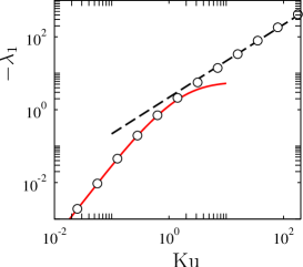
Figure 1: (Online color). Lyapunov exponent in one spatial dimension from direct numerical simulations of the model described in Section 2 (symbols), theory for large Ku (23), dashed line, and Padé-Borel resummation (19) of the perturbation series for small Ku (solid red line).

4 Two spatial dimensions

4.1 Small-Ku limit

Consider first the case of small Kubo numbers. Now there are two Lyapunov exponents to compute, describing the time evolution of the distance $|\delta\mbox{\boldmath$x$}_{t}|$ between two neighbouring particles and of the infinitesimal area element $\delta{\cal A}_{t}$ spanned by the separation vectors between three neighbouring particles:

$$\lambda_{1} = \lim_{t\rightarrow\infty}\frac{1}{t}\log\Big{|}\frac{\delta\mbox{\boldmath$x$}_{t}}{\delta\mbox{\boldmath$x$}_{0}}\Big{|}\,,$$ (24)

$$\lambda_{1}+\lambda_{2} = \lim_{t\rightarrow\infty}\frac{1}{t}\log\Big{|}\frac{\delta{\cal A}_{t}}{\delta{\cal A}_{0}}\Big{|}\,.$$ (25)

As in the one-dimensional case, these Lyapunov exponents are computed by linearising the equation of motion, Eq. (3) in this case. The dynamics at small separations $\delta\mbox{\boldmath$x$}$ between two neighbouring particles is

$$\frac{{\rm d}}{{\rm d}t}{\delta\mbox{\boldmath$x$}}_{t}=\mbox{Ku}\,\mathbb{A}(\mbox{\boldmath$x$}_{t},t)\,\delta\mbox{\boldmath$x$}_{t}\,.$$ (26)

Here $\mathbb{A}$ is the flow-gradient matrix with elements $A_{ij}\equiv\partial u_{i}/\partial x_{j}$. The Lyapunov exponents (25) are calculated from

$$\lambda_{1} =\mbox{Ku}\,\lim_{t\rightarrow\infty}\langle{\mbox{\boldmath$n$}}_{t}^{\mathrm{T}}\,\mathbb{A}(\mbox{\boldmath$x$}_{t},t)\,{\mbox{\boldmath$n$}}_{t}\rangle\,,$$ (27)

$$\lambda_{1}+\lambda_{2} =\mbox{Ku}\,\lim_{t\rightarrow\infty}\langle\mbox{Tr}\,\mathbb{A}(\mbox{\boldmath$x$}_{t},t)\rangle\,.$$ (28)

These relations are analogous to the one-dimensional Eq. (9). In Eq. (27), the vector ${\mbox{\boldmath$n$}}_{t}\equiv\delta\mbox{\boldmath$x$}_{t}/|\delta\mbox{\boldmath$x$}_{t}|$ is a time-dependent unit vector aligned with the separation vector between the two particles. Its dynamics follows from Eq. (26):

$$\dot{{\mbox{\boldmath$n$}}}_{t} =\mbox{Ku}\,\left[\mathbb{A}(\mbox{\boldmath$x$}_{t},t)\,{\mbox{\boldmath$n$}}_{t}-({\mbox{\boldmath$n$}}_{t}^{\mathrm{T}}\,\mathbb{A}(\mbox{\boldmath$x$}_{t},t)\,{\mbox{\boldmath$n$}}_{t})\,{\mbox{\boldmath$n$}}_{t}\right]\,.$$ (29)

The expressions (26) – (29) can be expanded analogously to the one-dimensional case described in the previous section. For the model flow given by Eqs. (4) and (5) we find to order $\mbox{Ku}^{8}$:

$$\lambda_{1} =\mbox{Ku}^{2}\frac{1-\beta^{2}}{1+\beta^{2}}-\mbox{Ku}^{4}\frac{6+7\beta^{2}-\beta^{4}}{(1+\beta^{2})^{2}}+\mbox{Ku}^{6}\frac{423+972\beta^{2}+597\beta^{4}+20\beta^{6}}{6(1+\beta^{2})^{3}}$$

$$-\mbox{Ku}^{8}\frac{164136+521517\beta^{2}+591081\beta^{4}+255803\beta^{6}+19927\beta^{8}}{144(1+\beta^{2})^{4}}$$ (30)

and

$$\lambda_{1}+\lambda_{2} =-\mbox{Ku}^{2}\frac{4\beta^{2}}{1+\beta^{2}}+2\mbox{Ku}^{4}\beta^{2}\frac{3+5\beta^{2}}{(1+\beta^{2})^{2}}-2\mbox{Ku}^{6}\beta^{2}\frac{33+123\beta^{2}+104\beta^{4}}{3(1+\beta^{2})^{3}}$$

$$+\mbox{Ku}^{8}\beta^{2}\frac{8718+51303\beta^{2}+92196\beta^{4}+51787\beta^{6}}{72(1+\beta^{2})^{4}}\,.$$ (31)

The lowest order, $\mbox{Ku}^{2}$, is consistent with the results quoted in LeJ85 ; Che98 ; Fal01 ; Bec04 ; Wil07 : the maximal Lyapunov exponent changes sign at $\beta_{\rm c}=1$. For $\beta=0$, Eqs. (30) and (31) yield the Lyapunov exponents for particles advected in a two-dimensional incompressible Gaussian random velocity field with finite Kubo number: $\lambda_{1}+\lambda_{2}=0$ (there cannot be clustering of particles advected in an incompressible flow), and Eq. (30) corresponds to the advective limit of Eq. (8) in Ref. Gus11 (the limit of zero Stokes number, $\mbox{St}\rightarrow 0$, must be taken in this equation describing the the maximal Lyapunov exponent of inertial particles). The series (30) and (31) are expected to be asymptotically divergent. Just as the one-dimensional result (16), Eqs. (30) and (31) are expected to fail at large Kubo numbers.

The series (30) and (31) can be resummed as in the one-dimensional case.

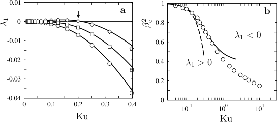
Figure 2: a Numerical results for maximal Lyapunov exponent for three different compressibilities (see Table 1): $\beta=0.91$ ($\Diamond$), $\beta=1$ ($\Box$), and $\beta=1.11$ ($\circ$). For $\beta=0.91$ the location of the path-coalescence transition is indicated by an arrow. Also shown are results of Padé-Borel resummations of the series (30) [solid lines]. b Shows location of the path-coalescence transition in the Ku-$\beta^{2}$ plane. Results of numerical simulations ($\circ$), resummation of the perturbation series (30) [solid line]. The dashed line corresponds to Eq. (32).

The results are seen in Fig. 2. Panel a shows results for the maximal Lyapunov exponent for $\beta$ close to $\beta_{\rm c}=1$ (the location of the path-coalescence transition in the limit of $\mbox{Ku}\rightarrow 0$). We see that at finite Kubo numbers the path-coalescence transition occurs at $\beta_{\rm c}(\mbox{Ku})<1$. Comparing the first two terms in Eq. (30) shows that to order $\mbox{Ku}^{2}$:

$$\beta_{\rm c}^{2}=1-6\mbox{Ku}^{2}\,.$$ (32)

For very small values of Ku this agrees with the numerical results in Fig. 2b. This panel shows the location of the path-coalescence transition in the Ku-$\beta^{2}$ plane. At large values of Ku, Padé-Borel resummations of the perturbation series (30) substantially improve the result. We observe good agreement between the numerical results and those of the resummation for values of Ku up to approximately $0.5$.

The results summarised in Fig. 2 show that at larger Kubo numbers less compressibility is needed to turn the maximal Lyapunov exponent negative. This is consistent with the behaviour observed at very large Kubo numbers: in the following section we show that the particles preferentially sample the attracting stagnation points of the velocity field in this limit. The contribution of these points increases as the Kubo number becomes larger. The observation that the effect of the compressible part of the velocity field is amplified at large Kubo numbers is consistent with numerical results in random renovating flows Mus13 . The dynamics of particles advected on the surface of a turbulent flow, by contrast, show a different behaviour Bof04 . In this case it is observed that the path-coalescence transition occurs at larger values of the compressibility for larger Kubo numbers. It would be of interest to determine which particular property of the turbulent flow gives rise to this effect.

4.2 Large-${\rm Ku}$ limit

The large-Ku limit in two-dimensional compressible flows is solved as in one spatial dimension. The required distribution $p(\mathbb{A})$ of the flow-gradient matrix $\mathbb{A}$ at $\mbox{\boldmath$u$}=0$ is found to be:

$$p(\mathbb{A})=\frac{\sqrt{(3+\beta^{2})(1+3\beta^{2})}}{\pi^{2}\beta}|\det\mathbb{A}|e^{-\mbox{\footnotesize\boldmath$a$}^{\mathrm{T}}\mathbb{C}^{-1}\mbox{\footnotesize\boldmath$a$}/2}\,,$$ (33)

where $\mbox{\boldmath$a$}=(A_{11},A_{12},A_{21},A_{22})$ and

$$\mathbb{C}=\frac{1}{2(1+\beta^{2})}\begin{pmatrix}1+3\beta^{2}&0&0&\beta^{2}-1\cr 0&3+\beta^{2}&\beta^{2}-1&0\cr 0&\beta^{2}-1&3+\beta^{2}&0\cr\beta^{2}-1&0&0&1+3\beta^{2}\end{pmatrix}\,.$$ (34)

The above expressions correspond to flows with both potential and solenoidal components because we expect that the expressions for the Lyapunov exponents derived below are not only valid for purely potential flows, but also yield good estimates for flows with a small solenoidal component.

We change coordinates $s_{\pm}=(A_{11}\pm A_{22})/2$ and $u_{\pm}=(A_{12}\pm A_{21})/2$ to obtain

$$p(s_{+},s_{-},u_{+},u_{-}) =\frac{\sqrt{(3+\beta^{2})(1+3\beta^{2})}}{4\pi^{2}\beta}|s_{+}^{2}+u_{-}^{2}-u_{+}^{2}-s_{-}^{2}|$$

$$\times\exp\left[-\frac{1+\beta^{2}}{2\beta^{2}}s_{+}^{2}-s_{-}^{2}-u_{+}^{2}-\frac{1+\beta^{2}}{2}u_{-}^{2}\right]\,.$$ (35)

The Lyapunov exponents are given by the eigenvalues of the strain matrix $\sigma_{\pm}=s_{+}\pm\sqrt{s_{-}^{2}+u_{+}^{2}-u_{-}^{2}}$ at the zeroes of $u$ subject to the constraint $\operatorname{\mathfrak{Re}}\,\sigma_{\pm}<0$. This condition is equivalent to the condition $\mbox{Tr}\mathbb{A}<0$ and $\det\mathbb{A}>0$ and can be expressed as

$$s_{+}<-\operatorname{\mathfrak{Re}}\sqrt{s_{-}^{2}+u_{+}^{2}-u_{-}^{2}}\,.$$ (36)

We have:

$$\lambda_{1,2} =4\mbox{Ku}\int_{-\infty}^{\infty}{\rm d}s_{+}{\rm d}s_{-}{\rm d}u_{+}{\rm d}u_{-}\,\Theta\Big{(}-\operatorname{\mathfrak{Re}}\sqrt{s_{-}^{2}+u_{+}^{2}-u_{-}^{2}}-s_{+}\Big{)}$$

$$\times\Big{(}s_{+}\pm\sqrt{s_{-}^{2}+u_{+}^{2}-u_{-}^{2}}\Big{)}p(s_{+},s_{-},u_{+},u_{-})\,.$$ (37)

The factor $4$ is a normalisation factor due to the fact that we only consider matrices $\mathbb{A}$ with $\operatorname{\mathfrak{Re}}\,\sigma_{\pm}<0$. Further $\Theta(z)$ takes the value $\Theta(z)=1$ when $z>0$, and zero otherwise. To evaluate the integral we change variables according to

$$\left\{\begin{array}[]{l}s_{-}=w\sqrt{1+\xi^{2}}\cos\varphi\cr u_{+}=w\sqrt{1+\xi^{2}}\sin\varphi\cr u_{-}=w\xi\end{array}\right.\,\mbox{ for }\Delta=s_{-}^{2}+u_{+}^{2}-u_{-}^{2}\geq 0$$ (41)

$$\left\{\begin{array}[]{l}s_{-}=w\xi\cos\varphi\cr u_{+}=w\xi\sin\varphi\cr u_{-}=w\sqrt{1+\xi^{2}}\end{array}\right.\,\mbox{\hskip 23.61583pt for }\Delta=s_{-}^{2}+u_{+}^{2}-u_{-}^{2}<0$$ (45)

with $0\leq w<\infty$, $-\infty<\xi<\infty$ and $0\leq\phi<2\pi$. Upon integrating over $\varphi$ and $\xi$ we obtain:

$$\lambda_{1,2} =2\mbox{Ku}\frac{\sqrt{1+3\beta^{2}}}{\sqrt{2\pi}\beta}\int_{-\infty}^{0}{\rm d}s_{+}\int_{0}^{\infty}\!\!\!{\rm d}w\,w\,\exp\Big{[}-\frac{\scriptstyle 1+\beta^{2}}{\scriptstyle 2\beta^{2}}s_{+}^{2}\Big{]}$$ (46)

$$\times\Big{\{}\Theta\Big{(}-\omega-s_{+}\Big{)}(s_{+}\mp\sqrt{w^{2}})|s_{+}^{2}-w^{2}|e^{-w^{2}}$$

$$+(s_{+}\mp\sqrt{-w^{2}})|s_{+}^{2}+w^{2}|{\rm erfc}\Big{[}\frac{\sqrt{\scriptstyle 3+\beta^{2}}w}{\scriptstyle\sqrt{2}}\Big{]}e^{w^{2}}\Big{\}}\,.$$

Performing the remaining integrals we find an approximation for the Lyapunov exponents:

$$\lambda_{1,2} =\frac{\mbox{Ku}}{2(1+\beta^{2})^{5/2}\sqrt{1+3\beta^{2}}\sqrt{\pi}}\Big{[}\sqrt{2}\beta(1+\beta^{2})^{3/2}(-2\mp 3+\beta^{2}(-2\mp 5))$$

$$\hskip 65.44142pt-2\sqrt{2}\beta^{3}\sqrt{3+\beta^{2}}(1+3\beta^{2})$$

$$\hskip 65.44142pt\mp(1+\beta^{2})(3+\beta^{2})(1+3\beta^{2})\arctan\Big{(}\sqrt{\frac{\scriptstyle 2\beta^{2}}{\scriptstyle 1+\beta^{2}}}\Big{)}\Big{]}\,.$$ (47)

The sum of the Lyapunov exponents is given by

$$\lambda_{1}+\lambda_{2} =-\frac{2\sqrt{2}\beta\mbox{Ku}}{(1+\beta^{2})^{5/2}\sqrt{1+3\beta^{2}}\sqrt{\pi}}\bigg{[}(1+\beta^{2})^{5/2}+\beta^{2}\sqrt{3+\beta^{2}}(1+3\beta^{2})\bigg{]}\,.$$ (48)

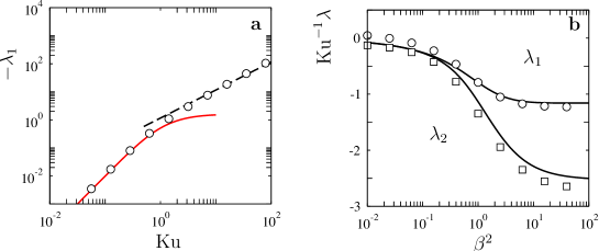
Figure 3: (Online color). a Maximal Lyapunov exponent from direct numerical simulations of the two-dimensional model described in Section 2 (symbols) in the limit $\beta\rightarrow\infty$. Results from resummation of perturbation theory in Ku (30) (solid red line) and asymptotic result for large Ku (49) (dashed line). b Lyapunov exponents for $\mbox{Ku}=100$ as a function of $\beta^{2}$. Numerical results: $\lambda_{1}$ ($\circ$) and $\lambda_{2}$ ($\Box$), theoretical results, Eqs. (47,48), solid lines.

Eqs. (47) and (48) give estimates for the Lyapunov exponents for large but finite values of Ku, as opposed to Eqs. (30)-(31) that give the corresponding expressions for small values of Ku.

Let us consider the purely compressible limit $\beta\to\infty$ in (47) and (48):

$$\lambda_{1,2} \sim\frac{1}{\sqrt{12\pi}}\mbox{Ku}\Big{[}-8\sqrt{2}\pm(5\sqrt{2}-3\arctan(\sqrt{2}))\Big{]}\,,$$ (49)

$$\lambda_{1}+\lambda_{2} \sim-\frac{16}{\sqrt{6\pi}}\mbox{Ku}\,.$$ (50)

Both the maximal exponent $\lambda_{1}$ and the sum $\lambda_{1}+\lambda_{2}$ are negative in this limit, as expected: the particles converge to the minima of $V(\mbox{\boldmath$x$},t)=-\psi(\mbox{\boldmath$x$},t)$ at large Kubo numbers. Eqs. (49) and (50) predict that the Lyapunov exponents scale as Ku for large values of Ku. At small values of Ku, by contrast, the scaling is $\mbox{Ku}^{2}$ as Eqs. (30) and (31) show. Fig. 3a shows the asymptotic result (49) for $\lambda_{1}$ in comparison with results of numerical simulations for particles suspended in a two-dimensional compressible (purely potential) velocity field. We observe good agreement.

We expect Eqs. (47) and (48) to give reliable estimates when the particles are typically found very close to the minima of the potential. Fig. 3b shows numerical results for the Lyapunov exponents at $\mbox{Ku}=100$ in partially compressible flows as a function of $\beta^{2}$, compared with Eqs. (47) and (48). We observe that Eqs. (47) and (48) yield reasonable estimates even for small degrees of compressibility. We note that the theory must fail in the incompressible limit ($\beta=0$), and is only an approximation for finite values of $\beta$. The results show, however, that the dynamics is dominated by the attracting stagnation points of the velocity field at large Kubo numbers.

5 Conclusions

In this paper we have computed the Lyapunov exponents of small tracer particles advected in one- and two-dimensional compressible random velocity fields at finite Kubo numbers. For small Kubo numbers we have obtained results by Padé-Borel resummation of perturbation expansions in Ku. For large Kubo numbers we have computed the Lyapunov exponents using the Kac-Rice formula. At finite Kubo numbers the resulting Lyapunov exponents are determined by the details the velocity-field fluctuations (at small values of Ku by the Eulerian $n$-point functions of the velocity field and its derivatives, and at large values of Ku by the statistics of its stagnation points). Our results generalise earlier results LeJ85 ; Che98 ; Fal01 ; Bec04 ; Wil07 for compressible flows obtained in the limit $\mbox{Ku}\rightarrow 0$ to finite Kubo numbers. We find that $\lambda\sim\mbox{Ku}^{2}$ as $\mbox{Ku}\rightarrow 0$ and $\lambda\sim\mbox{Ku}$ at large (but finite) values of Ku. We have demonstrated that the analytical results are in good agreement with results of numerical simulations, and provide accurate estimates of the location of the path-coalescence transition for particles advected in compressible flows with finite Kubo numbers.

The limit $\beta\rightarrow 0$ at large Kubo numbers remains to be analysed. For small values of $\beta$ the stagnation points determining the Lyapunov exponents attract only weakly because the corresponding potential minima are shallow: Ku must be very large for the minima not to disappear before particles are attracted. In this limit a fraction of particles spends an appreciable amount of time on close-to closed orbits. This contribution is not accounted for in the derivation of Eqs. (47) and (48). For this reason these results are approximate, unless $\beta$ is infinity. At $\beta=0$ and $\mbox{Ku}=\infty$ the two-dimensional dynamics (3) corresponds to a one-dimensional Hamiltonian system. In this case the Lyapunov exponents must vanish. It would be interesting (but outside the scope of this paper) to consider, if possible, an expansion around this steady case.

We conclude by commenting on two further implications of our results. First, as mentioned in the introduction, spatial clustering of weakly inertial particles in incompressible velocity fields is often described in terms of a model where the particles are advected in a ‘synthetic’ velocity field with a small compressible component (due to the particle inertia). It is known that this approach must fail when the inertia is large (because of the formation of caustics). But there is also a problem in the small-inertia limit. Consider the sum of the Lyapunov exponents for inertial particles in a Gaussian random flow at finite Kubo numbers, Eq. (9) in Ref. Gus11 :

$$\lambda_{1}+\lambda_{2}=-6\mbox{Ku}^{4}\frac{\mbox{St}^{2}(1+3\mbox{St}+\mbox{St}^{2})}{(1+\mbox{St})^{3}}+\ldots$$ (51)

Here St is the ‘Stokes number’ characterising the importance of particle inertia. The limit $\mbox{St}=0$ corresponds to advective dynamics. Comparing Eq. (51) with the leading-order term of Eq. (31) at small St and $\beta$ would lead us to conclude that weakly inertial particles are described by an advective model with ‘effective compressibility’ $\beta=\sqrt{3/2}\,\mbox{Ku}\mbox{St}$. But this does not give the correct result for $\lambda_{1}$ (c.f. Eq. (8) in Ref. Gus11 ), neither does this correspondence yield consistent results for terms of higher order in Ku (determined by higher-order correlation functions of the velocity field). This shows that care is required when approximating the dynamics of weakly inertial particles by advection in a weakly compressible velocity field: in general the statistics obtained by sampling along particle trajectories with actual inertial velocities, and in the effective compressible velocity field are different.

Second, a related Ku-expansion was recently used to compute the tumbling rate of small axisymmetric particles in three-dimensional random velocity fields at finite Kubo numbers Gus13a . It turns out that the resummation works well also for the series expansion of the tumbling rate.

- [1] J. Sommerer and E. Ott. Particles floating on a moving fluid: A dynamically comprehensible physical fractal. Science, 259:334, 1993.
- [2] J. Kaplan and J. A. Yorke. Chaotic behavior of multidimensional difference equations. Springer Lecture Notes in Mathematics, 730:204–227, 1979.
- [3] M. Wilkinson and B. Mehlig. Path coalescence transition and its applications. Phys. Rev. E, 68:040101(R), 2003.
- [4] M. Wilkinson, B. Mehlig, K. Gustavsson, and E. Werner. Clustering of exponentially separating trajectories. European Physical Journal B, 85:18, 2012.
- [5] G. Boffetta, J. Davoudi, B. Eckhardt, and J. Schumacher. Tracer dynamics in a turbulent field: influence of time correlations. Phys. Rev. Lett., 93:134501, 2004.
- [6] J. R. Cressman, J. Davoudi, W. I. Goldberg, and J. Schumacher. Eulerian and Lagrangian studies in surface flow turbulence. New J. Phys., 6:53, 2004.
- [7] J. Bec. Fractal clustering of inertial particles in random flows. Phys. Fluids, 15:81–84, 2003.
- [8] M. Wilkinson, B. Mehlig, S. Östlund, and K. P. Duncan. Unmixing in random flows. Phys. Fluids, 19:113303, 2007.
- [9] E. Balkovsky, G. Falkovich, and A. Fouxon. Intermittent distribution of inertial particles in turbulent flows. Phys. Rev. Lett., 86:2790–3, 2001.
- [10] M. R. Maxey. The gravitational settling of aerosol particles in homogeneous turbulence and random flow fields. J. Fluid Mech., 174:441–465, 1987.
- [11] G. Falkovich, A. Fouxon, and G. Stepanov. Acceleration of rain initiation by cloud turbulence. Nature, 419:151, 2002.
- [12] M. Wilkinson and B. Mehlig. Caustics in turbulent aerosols. Europhys. Lett., 71:186–192, 2005.
- [13] K. Gustavsson and B. Mehlig. Inertial-particle dynamics in turbulent flows: caustics, concentration fluctuations, and random uncorrelated motion. New J. Phys., 14:115017, 2012.
- [14] K. Gustavsson and B. Mehlig. Distribution of velocity gradients and rate of caustic formation in turbulent aerosols at finite Kubo numbers. Phys. Rev. E, 87:023016, 2013.
- [15] M. Wilkinson, B. Mehlig, and V. Bezuglyy. Caustic activation of rain showers. Phys. Rev. Lett., 97:048501, 2006.
- [16] K. Gustavsson and B. Mehlig. Distribution of relative velocities in turbulent aerosols. Phys. Rev. E, 84:045304, 2011.
- [17] K. Gustavsson and B. Mehlig. Relative velocities of inertial particles in turbulent aerosols. arXiv:1307.0462, 2013.
- [18] Y. Le Jan. On isotropic Brownian motions. Z. Wahrsch. verw. Gebiete, 70:609, 1985.
- [19] M. Chertkov, I. Kolokov, and M. Vergassola. Inverse versus direct cascades in turbulent advection. Phys. Rev. Lett. 80:512–515, 1998.
- [20] G. Falkovich, K. Gawedzki, and M. Vergassola. Particles and fields in fluid turbulence. Rev. Mod. Phys., 73:913, 2001.
- [21] J. Bec, K. Gawedzki, and P. Horvai. Multifractal clustering in compressible flows. Phys. Rev. Lett., 92:224501, 2004.
- [22] B. Mehlig and M. Wilkinson. Coagulation by random velocity fields as a Kramers problem. Phys. Rev. Lett., 92:250602, 2004.
- [23] K. Duncan, B. Mehlig, S. Östlund, and M. Wilkinson. Clustering in mixing flows. Phys. Rev. Lett., 95:240602, 2005.
- [24] M. Chertkov, G. Falkovich, I. Kolokov, and V. Lebedev. Theory of random advection in two dimensions. Int. J. Mod. Phys. B, 10:2273–2309, 1996.
- [25] G. Falkovich, S. Musacchio, L. Piterbarg, and M. Vucelja. Inertial particles driven by a telegraph noise. Phys. Rev. E 76:026313, 2007.
- [26] G. Falkovich, and M. M. Alfonso. Fluid-particle separation in a random flow described by the telegraph model. Phys. Rev. E 76:026312, 2007.
- [27] A. Dhanagare, S. Musacchio, D. Vincenzi et al.. Clustering in time-correlated compressible flows. 2013.
- [28] K. Gustavsson and B. Mehlig. Ergodic and non-ergodic clustering of inertial particles. Europhys. Lett., 96:60012, 2011.
- [29] M. Wilkinson. Lyapunov exponent for small particles in smooth one-dimensional flows. J. Phys. A, 44:045502, 2011.
- [30] M. Kac. On the average number of real roots of a random algebraic equation. Bull. Am. Math. Soc., 49:314, 1943.
- [31] S. O. Rice. Mathematical theory of random noise. Bell System Tech. J., 25:46, 1945.
- [32] B. Mehlig, M. Wilkinson, K. Duncan, T. Weber, and M. Ljunggren. Aggregation of inertial particles in random flows. Phys. Rev. E, 72:051104, 2005.
- [33] K. Gustavsson. Advective collisions in random flows. Licenciate thesis, University of Gothenburg, 2009.
- [34] J. P. Boyd. The devil’s invention: asymptotic, superasymptotic and hyperasymptotic series. Acta Applicandae, 56:98, 1999.
- [35] C. M. Bender and S. A. Orszag. Advanced Mathematical Methods for Scientists and Engineers. McGraw-Hill, New York, USA, 1978.
- [36] K. Gustavsson, J. Einarsson, and B. Mehlig. Tumbling of axisymmetric particles in turbulent and random flows. arXiv:1305.1822, 2013.