In-out decomposition of boundary integral equations

Abstract

We propose a reformulation of the boundary integral equations for the Helmholtz equation in a domain in terms of incoming and outgoing boundary waves. We obtain transfer operator descriptions which are exact and thus incorporate features such as diffraction and evanescent coupling; these effects are absent in the well known semiclassical transfer operators in the sense of Bogomolny. It has long been established that transfer operators are equivalent to the boundary integral approach within semiclassical approximation. Exact treatments have been restricted to specific boundary conditions (such as Dirichlet or Neumann). The approach we propose is independent of the boundary conditions, and in fact allows one to decouple entirely the problem of propagating waves across the interior from the problem of reflecting waves at the boundary. As an application, we show how the decomposition may be used to calculate Goos-Hänchen shifts of ray dynamics in billiards with variable boundary conditions and for dielectric cavities.

1 Introduction

The transfer operator formalism proposed by Bogomolny [1] has offered a very powerful platform for the application of semiclassical methods to complex quantum and wave problems. It has long been recognised that, in the special case of cavity problems such as quantum billiards or dielectric resonators, the transfer operator is intimately connected with boundary integral methods, which provide the most effective means of exact, numerical solution. Boasman established this connection explicitly in [2] for quantum billiards, recasting the boundary integral equations as the application of a transfer operator to the wavefunction on the boundary (in the case of Dirichlet boundary conditions) or to its normal derivative (in the case of Neumann boundary conditions). Subsequent development using Fredholm theory can be found in [3, 4, 5, 6, 7], particularly on the Dirichlet case. If the boundary conditions are more general, however, it is less clear how the connection can be made exactly, although the approaches are easily related semiclassically (see [8, 9, 10, 11], for example). In this paper we propose that a decomposition of the wavefunction at the boundary into incoming and outgoing components, defined in detail following a separation of the Green function into its regular and singular parts, provides a natural means of establishing this connection beyond leading semiclassical approximations.

Semiclassical methods originating in the field of quantum chaos have found widespread application in classical wave problems with complex or chaotic ray limits. In particular in the context of vibro-acoustics [12] or for electromagnetic wave fields [13], cavity problems with a variety of boundary conditions are prevalent. An efficient phase space flux method, the so-called Dynamical Energy Analysis (DEA), has been developed recently, predicting wave energy transport through complex structures and domains based on trajectory calculations [14, 15]. A more explicit connection to boundary integral equations in terms of transfer operator methods and incoming and outgoing waves is a key ingredient for constructing hybrid DEA - wave methods [16]. This is especially valuable where semiclassically higher-order mechanisms such as diffraction or evanescent coupling are important. In addition, one often encounters the situation where semiclassical ideas provide a simple qualitative description of the problem, but where the wavelength is too large to use them for reliable quantitative predictions. A semiclassically-motivated decomposition such as proposed in this paper can then lead to an efficient implementation of fully wave-based calculations. Our treatment of the Goos-Hänchen shift is one example of this latter case; simplistic ray-dynamical models break down in the most important regions of phase space but nevertheless provide a very useful conceptual basis on which to found more accurate calculations using, for example, the method proposed here.

Figure 1: In this paper, $\psi_{-}(s)$ denotes the component of the boundary solution corresponding to the part of the wave approaching the boundary from the interior of the domain $\Omega$ and $\psi_{+}(s)$ denotes the component leaving the boundary towards the interior.

The main technical issue to be addressed in this paper is how to decompose the wave solution at the boundary into a component approaching the boundary and a component leaving it (see Fig. 1). This decomposition is automatically achieved in the context of semiclassical approximation when the wavefunction takes the form of an eikonal ansatz, where ray direction allows us to select incoming and reflected wave components. For problems which are not semiclassical, or where the solution cannot easily be represented in eikonal form, the decomposition is less obvious. We propose that the outgoing wave $\psi_{+}(s)$ should be defined simply as the contribution to the boundary integral equation arising from an appropriately defined singular part of the Green function. The motivation for this definition is that, just inside $\Omega$, the corresponding contribution to the boundary integral equation is dominated by the part of the boundary nearby and represents a wave emerging from the boundary towards the interior. This definition is consistent within semiclassical approximation with the obvious decomposition according to the direction of rays. It also reproduces expected results in the one-dimensional case and in a sense our calculation amounts to a generalisation to higher dimensions of the scattering approach normally used on quantum graphs [17, 18].

There remains some ambiguity, however, arising from the possibility of defining the singular part of the Green function in different ways. The simplest definition having the correct semiclassical limit is to define the singular part to correspond to the Green function obtained by replacing the boundary locally by its tangent line or plane. The resulting decomposition can also be motivated by a transformation to momentum-represention of the solution along the boundary. This provides a separation according to ray direction as is automatically achieved using an eikonal ansatz. We will refer to this as the primitive decomposition. The primitive decomposition is shown in [19] to allow the treatment of diffractive effects from discontinuous boundary conditions, for example, or to provide a basis for the semiclassical coupling of transfer operators between multiple domains with different local wave number.

The primitive decomposition displays singularities in momentum representation near the case of critical reflection where waves arrive at the boundary almost tangentially. Although one might still define an associated transfer operator before semiclassical approximation, such singularities will at least lead to issues such as slow convergence. The regime of near tangential angle of incidence is particularly important when describing leakage from dielectric resonators. Here the “critical line” in phase space, along which refractive escape switches on, plays an important role in emission patterns and decay rates. We therefore propose a second separation of the Green function into singular and regular parts based on a splitting of the boundary integral into distinct contours in the complex plane, one of which captures the Green function’s singularity. We call this second decomposition the regularised decomposition. It successfully accounts for the important effects of boundary curvature at critical reflection and remains well-behaved when waves arrive nearly tangentially. We examine the regularised decomposition in detail for the special case of circular cavities.

We find in general that the boundary integral equations can be cast in the form

$$\psi_{-}=\hat{S}\psi_{+},$$ (1)

where the operator $\hat{S}$ depends on the geometry of the domain but is completely independent of the boundary conditions: in this paper we will refer to $\hat{S}$ as the shift operator. This equation is naturally interpreted as saying that $\psi_{-}$ is obtained by propagating the outgoing wave $\psi_{+}$ across the interior until it returns to the boundary as an incoming wave. For the case of circular cavities we provide explicit, closed-form expressions for $\hat{S}$. We emphasise that this is achieved even in the presence of variable boundary conditions such as those treated in [20, 21], where the problem as a whole is nonintegrable. We show that, closing the system by using the boundary conditions to relate the outgoing to the incoming component by a reflection operator $\hat{r}$, we arrive at an overall transfer operator taking the form of a stroboscopic map $\hat{T}=\hat{r}\hat{S}$. Semiclassical treatments provide a simple interpretation of $\hat{r}$ as acting on rays by a Goos-Hänchen shift, so that the overall operator offers a simple explanation of the Goos-Hänchen-perturbed ray dynamics of the type used in [22, 23, 24, 25] to treat dielectric cavities. Furthermore, the regularised decomposition allows a more complete treatment of the case of critical reflection (or refraction), albeit in that case with a less simple interpretation in terms of rays.

At a formal level, the construction of a transfer operator as a map between boundary functions is similar to the scattering-matrix approach developed by Smilansky and coworkers [26, 27, 28] or the transfer-operator approach by Prosen [29, 30, 31]. Similar to our approach, a wave solution is decomposed in those calculations into components passing in either direction through a surface of section cutting through the domain of interest or split into an incoming and outgoing wave component at (parts of) the boundary of a cavity. The formalism by Smilansky et al and Prosen rely on being able to construct explicitly a scattering matrix for the regions lying to either side of a surface of section. They are thus most natural when decomposing the problem in hand into two ’half-problems’ separated by the surface of section. Such a treatment becomes less obvious when using as the section the full boundary of a closed cavity, the most natural surface of section when starting from boundary integral equations. It is worth mentioning that the transfer operator construction proposed by Prosen [29, 30, 31] is similar to the ’primitive decomposition’ introduced above. Prosen developed a more general approach dealing also with smooth potentials, but the restricted circumstances we assume here allows a simpler derivation and a generalisation to a regularised decomposition which deals better with the case of critical reflection, for example.

The emphasis in this paper is quite different, however. We argue that, starting from the boundary integral equation, one can naturally decompose the Green functions occurring there into singular and regular components that are closely related to the incoming and outgoing component of the boundary wave function. The regularised decomposition provides in particular a description which stays regular at grazing incident angles and which makes it possible to distinguish propagating and evanescent (exponentially decaying) wave contributions without explicitly referring to a (scattering) channel basis.

The regularised decomposition approach applies in it simplest form to cavities that have convex, analytic boundaries. The boundary needs to be analytic so that the contour integration methods used to define singular and regular parts of the Green operators can be defined. Assuming that the boundary is convex allows a more direct leading semiclassical description of the shift operator $\hat{S}$ in terms of the Green operators, without the need to account explicitly for the cancellation of ghost orbits (see [7]). Treatments of piecewise analytic boundaries, with a more explicit account of corners, and of nonconvex billiards will be the subject of future investigation.

We conclude this section by summarising the content of the paper. We begin in Sec. 2 by establishing notation and outlining the main technical features of the calculation. The use of the decomposition of Green operators into local and nonlocal parts to define incoming and outgoing waves is illustrated in Sec. 3 for the one-dimensional case, where calculations are elementary. This is generalised to two-dimensional cavities in Sec. 4 using the primitive decomposition. The regularised decomposition, taking more explicit account of boundary curvature, is treated in Sec. 5. Finally some model two-dimensional cases are examined in Secs. 6 and 7, providing in particular explicit analytic descriptions of the shift operators for the circle, and conclusions are offered in Sec. 8.

2 Overview

We now summarise the main features of our calculation, concentrating on the case of two-dimensional cavities to fix notation. We emphasise that the main ideas in this section generalise to higher dimensions.

Let $\psi({\bf x})$ satisfy the Helmholtz equation

$$-\nabla^{2}\psi=k^{2}\psi$$

in the (two-dimensional) domain $\Omega$. We use the same symbol $\psi(s)$ to represent the restriction of the solution to the boundary $\partial\Omega$, on which $s$ is an arc-length coordinate, and denote the normal derivative by

$$\mu(s)={{\partial\psi}\over{\partial n}}.$$

Let $G_{0}({\bf x},{\bf x}^{\prime};k)$ denote the free-space Green function satisfying $(-\nabla^{2}-k^{2})G_{0}({\bf x},{\bf x}^{\prime};k)=\delta({\bf x}-{\bf x}^{\prime})$. The boundary integral equation for $\psi$ may then be written formally as

$$\psi = \hat{G}_{0}\mu-\hat{G}_{1}\psi,$$ (2)

where we denote the Green operators

$$\hat{G}_{0}\mu(s) = \lim_{{\bf x}\to s}\int_{\partial\Omega}G_{0}({\bf x},s^{\prime};k)\mu(s^{\prime}){\rm d}s^{\prime}$$ (3)

$$\hat{G}_{1}\psi(s) = \lim_{{\bf x}\to s}\int_{\partial\Omega}{{\partial G_{0}({\bf x},s^{\prime};k)}\over{\partial n^{\prime}}}\psi(s^{\prime}){\rm d}s^{\prime},$$ (4)

in which ${\bf x}$ denotes a generic point in the interior of $\Omega$ and $s$ and $s^{\prime}$ label points on the boundary.

Figure 2: The wave emerging from the part of the boundary near ${\bf x}$, as ${\bf x}\to{\bf x}(s)$, provides a natural definition of the outgoing component $\psi_{+}$. We define this more directly as the contribution from the singular part of the Green function. The regular remainder defining $\psi_{-}$ represents the contributions originating from the rest of the boundary, arriving at $s$ having passed through the interior.

The key step in the transformation we propose is to perform a basis change

$$\left(\begin{array}[]{c}\psi(s)\\ \mu(s)\end{array}\right)\to\left(\begin{array}[]{c}\psi_{-}(s)\\ \psi_{+}(s)\end{array}\right)$$

in which we replace the boundary wavefunction $\psi(s)$ and normal derivative $\mu(s)$ by incoming and outgoing components $\psi_{-}(s)$ and $\psi_{+}(s)$, defined in the simplest implementation so that

$$\psi(s)=\psi_{-}(s)+\psi_{+}(s).$$ (5)

Motivated by the schematic picture of Fig. 2, we argue that $\psi_{+}(s)$ is naturally defined as corresponding to the part of the boundary integral in which $s^{\prime}$ approaches $s$. This should capture in particular the singularity of the 2D Green function,

$$G_{0}(s,s^{\prime},k)\sim-\frac{1}{2\pi}\log(k|s-s^{\prime}|)$$ (6)

as $s^{\prime}\to s$. We therefore separate the Green operators into “singular” and “regular” parts,

$$\hat{G}_{0}=\hat{G}^{\rm sing}_{0}+\hat{G}^{\rm reg}_{0},$$ (7)

(with an analogous decomposition of $\hat{G}_{1}$), where $\hat{G}_{0}^{\rm sing}$ is an operator which should give the contribution to the boundary integral from $s^{\prime}$ near $s$ and should in particular account for the singularity (6). We then define

$$\psi_{+}=\hat{G}^{\rm sing}_{0}\mu-\hat{G}^{\rm sing}_{1}\psi,$$ (8)

and

$$\psi_{-}=\hat{G}^{\rm reg}_{0}\mu-\hat{G}^{\rm reg}_{1}\psi.$$ (9)

Note that, in the schematic picture of Fig. 2, $\psi_{-}(s)$ now collects the contributions to the boundary integral equation from the remainder of the boundary, arriving at $s$ having crossed the interior of the cavity. This is consistent with our requirement that $\psi_{-}$ should represent the part of the solution that is incoming at the boundary.

We discuss in the coming sections the detailed calculation that arises once the decomposition (7) has been defined more explicitly. Here we summarise the main conclusion, which is, that the boundary integral equation (2), expressed in terms of $\psi_{+}$ and $\psi_{-}$, can be recast formally as equation (1). We emphasise that this equation derives entirely from the boundary integral equation and has nothing to do with the boundary conditions. For a given domain $\Omega$, we get the same shift operator $\hat{S}$ in (1) regardless of whether Dirichlet, Neumann or any other boundary condition is imposed.

The boundary conditions provide us with a second, independent relationship between $\psi_{-}$ and $\psi_{+}$. Suppose that the boundary conditions are prescribed in the form of a linear relationship between $\psi$ and $\mu$ on $\partial\Omega$. (This assumption must be modified for the treatment of dielectric and other problems where coupling to an exterior solution is involved, as described in Sec. 7). We re-express this in terms of the functions $\psi_{-}(s)$ and $\psi_{+}(s)$ as

$$\psi_{+}=\hat{r}\psi_{-}$$

where we call $\hat{r}$ the reflection operator, for obvious reasons. Combined with (1), we find

$$\psi_{+}=\hat{T}\psi_{+},$$

where

$$\hat{T}=\hat{r}\hat{S}$$ (10)

is the transfer operator for the problem as a whole. Eigenvalues are found by solving the secular equation

$${\rm det}\,(\hat{I}-\hat{T}(k))=0.$$

We find indeed that, when semiclassical approximations are used for $\hat{S}$ and $\hat{r}$, we recover the usual transfer operator expected from [1] (up to a simple conjugation of the operators involved: see B).

Note that the transfer operator $\hat{T}$ is presented as a stroboscopic map, composing the shift operator $\hat{S}$, determined entirely by the shape of $\Omega$, with the reflection operator $\hat{r}$, accounting for boundary conditions. In semiclassical approximation, $\hat{S}$ is determined by the usual ray dynamics assuming specular reflection at each bounce. The reflection operator can be accounted for in this picture simply by adding appropriate phases as rays are reflected from the boundary. An alternative point of view, which has been found to be fruitful in the treatment of dielectric problems, for example, is to regard the variable reflection phases inherent in $\hat{r}$ as adding a perturbation to the usual ray dynamics in the form of a Goos-Hänchen shift [22, 23, 24, 25, 32, 33]. In our approach, this is easily understood from the stroboscopic nature of the full operator $\hat{T}$. Writing $\hat{r}$ formally as an exponential

$$\hat{r}={\rm e}^{-{\rm i}k\hat{h}},$$ (11)

and using an analogy with quantum mechanics in which $k$ plays the role of $1/\hbar$, we can interpret $\hat{h}$ as the generator of $\hat{r}$. The corresponding effect on rays is obtained simply by replacing $\hat{h}$ by a symbol $h(s,p)$ on the boundary phase space and using this as a classical Hamiltonian. Note that, because the reflection phases are formally of $O(1)$ in an eikonal expansion in $1/k$, the Hamiltonian $h(s,p)$ so defined is small and therefore only perturbs the main ray dynamics (and that is why we are equally entitled to leave the ray dynamics alone and incorporate reflection phases instead in the next-to-leading, amplitude-transport phase of the eikonal expansion [34]).

3 The one-dimensional case and quantum graphs

In order to motivate equations (8) and (9) further as a means of decomposing the boundary solution into incoming and outgoing components, we consider now the one-dimensional case. The most direct analogue leads very simply to the standard picture one uses for the wave dynamics on quantum graphs [17].

Figure 3: A schematic illustration is given of the diagonal and nondiagonal contributions to the boundary integral equation in the one-dimensional case. As the interior point $x$ approaches the boundary point $a$, the off-diagonal contribution $\psi_{-}$ to (2) represents a wave originating at $0$ and moving towards the selected boundary point $a$. This diagonal contribution $\psi_{+}$ represents a wave emerging from $a$ and moving away from the boundary.

Consider first the case of an interval $(0,a)$, illustrated in Fig. 3. Here the boundary solution can be represented by the two-component vectors

$$\psi=\left(\begin{array}[]{c}{\psi(0)}\\[9.0pt] {\psi(a)}\end{array}\right)\qquad\mbox{and}\qquad\mu=\left(\begin{array}[]{c}{\mu(0)}\\[9.0pt] {\mu(a)}\end{array}\right),$$

while, from the one-dimensional Green function

$$G_{0}(x,x^{\prime};k)=\frac{{\rm i}}{2k}{\rm e}^{{\rm i}k|x-x^{\prime}|},$$ (12)

one finds that the Green operators can be represented by the $2\times 2$ matrices

$$G_{0}=\frac{{\rm i}}{2k}\left(\begin{array}[]{cc}1&\rme^{{\rm i}ka}\\[3.00003pt] \rme^{{\rm i}ka}&1\end{array}\right)=\frac{{\rm i}}{2k}\left(I+S\right)$$ (13)

and

$$G_{1}=-\frac{1}{2}\left(\begin{array}[]{cc}1&\rme^{{\rm i}ka}\\[3.00003pt] \rme^{{\rm i}ka}&1\end{array}\right)=-\frac{1}{2}\left(I+S\right),$$ (14)

where $I$ is the identity matrix and

$$S=\left(\begin{array}[]{cc}0&\rme^{{\rm i}ka}\\[3.00003pt] \rme^{{\rm i}ka}&0\end{array}\right)$$ (15)

will be found to play the role of the shift operator.

In this one-dimensional case, instead of separating the Green function into a singular and a regular part, as in (7), we separate the diagonal from the nondiagonal part

$$G_{0}=G^{\rm diag}_{0}+G^{\rm non-diag}_{0}.$$ (16)

That is, the role played in higher dimensions by the singular part (as $s^{\prime}\to s$) of the Green function is in one dimension taken over by the diagonal part (in which $s^{\prime}=s$). Then, defining

$$\psi_{+}=G^{\rm diag}_{0}\mu-G^{\rm diag}_{1}\psi=\frac{{\rm i}}{2k}\mu+\frac{1}{2}\psi,$$ (17)

and

$$\psi_{-}=G^{\rm non-diag}_{0}\mu-G^{\rm non-diag}_{1}\psi=\frac{{\rm i}}{2k}S\mu+\frac{1}{2}S\psi,$$ (18)

in analogy with (8) and (9), we find that the boundary integral equation (2) becomes

$$\psi_{-}=S\psi_{+}.$$

Note that in the case of quantum graphs we simply apply the same calculation independently to each bond and find an overall shift operator with diagonal blocks of the form (15). The problem is closed by applying boundary conditions at vertices to provide scattering operators that generalise $\hat{r}$ in (10) and couple the bond-labelled blocks of $\hat{S}$.

4 The primitive decomposition

The simplest decomposition in the two-dimensional case is obtained by defining the singular part of the Green operator to be the result of replacing the boundary locally by its tangent line, as illustrated in Fig. 4.

Figure 4: Illustration of the local replacement of the boundary (curved solid line) with the tangent (vertical dashed line) at $s$.

Before taking the limit, the kernel of the full Green operator entering (3) takes in 2D the form

$$G_{0}({\bf x},s^{\prime};k)=\frac{{\rm i}}{4}H_{0}(kL({\bf x},s^{\prime})),$$

where $L({\bf x},s^{\prime})$ denotes the distance between the generic interior point ${\bf x}$ and the boundary point $s^{\prime}$ and $H_{0}(z)$ is the outgoing Hankel function. If the boundary is replaced by the tangent line at $s$, (see Fig. 4), this distance can be written

$$L({\bf x},s^{\prime})\sim\sqrt{(s-s^{\prime})^{2}+\varepsilon^{2}},$$

where $\varepsilon$ denotes the normal distance from ${\bf x}$ to $s$. We define a corresponding singular component of the Green operator by

$$\hat{G}_{0}^{\rm sing}\mu(s)=\lim_{\varepsilon\to 0}\frac{{\rm i}}{4}\int_{-\infty}^{\infty}H_{0}\left(k\sqrt{(s-s^{\prime})^{2}+\varepsilon^{2}}\right)\mu(s^{\prime})\rmd s^{\prime}.$$ (19)

The boundary function $\mu(s)$ entering the integrand in (19) and in analogous equations below is here understood as being the periodic extension of the true boundary function onto the real line with period equal to the perimeter of $\partial\Omega$. (This is understood to hold both for open and closed boundaries in order to unify notation.)

This operator takes a remarkably simple form when expressed in a Fourier basis (or, in quantum mechanical language, a momentum representation):

$$\hat{G}^{\rm sing}_{0}=\frac{{\rm i}}{2k\hat{P}},$$ (20)

where

$$\hat{P}=\sqrt{1-\hat{p}^{2}}$$ (21)

formally defines a normal momentum operator and

$$\hat{p}=\frac{1}{{\rm i}k}\frac{\partial}{\partial s}$$

denotes a tangential momentum operator. More precisely, the action of the operator $\hat{P}$ on a function $\psi(s)$ is defined with respect to the Fourier transform

$$\varphi(p)=\int_{-\infty}^{\infty}\rme^{-{\rm i}kps}\psi(s)\rmd s$$ (22)

to be

$$\hat{P}\psi(s) = \frac{k}{2\pi}\int_{-\infty}^{\infty}\rme^{{\rm i}kps}\sqrt{1-p^{2}}\,\varphi(p)\rmd p,$$ (23)

where integration is over a contour in the complex $p$-plane that passes above the branch singularity $p=-1$ and below the branch singularity at $p=1$. The singular part of the operator $\hat{G}_{1}$ is even simpler:

$$\hat{G}_{1}^{\rm sing}=-\frac{1}{2}\hat{I},$$ (24)

where $\hat{I}$ is the identity operator. These relations are derived explicitly in A and reconfirm the well-known jump condition important to boundary integral methods more generally.

The outgoing wave defined in (8) can now be written

$$\psi_{+}=\frac{{\rm i}}{2k}\frac{1}{\hat{P}}\mu+\frac{1}{2}\psi,$$

providing a two-dimensional generalisation of (17). Together with the condition $\psi=\psi_{+}+\psi_{-}$, this implies

$$\mu={\rm i}k\hat{P}\left(\psi_{-}-\psi_{+}\right),$$

which is what one might expect intuitively on the basis of a Fourier representation of the solution near the boundary: a boundary solution $\psi(s)={\rm e}^{{\rm i}kps}$ extends to an interior solution $\psi_{\pm}({\bf x})\simeq\exp[{{\rm i}k(ps\mp\sqrt{1-p^{2}}n)}]$ near the boundary, where $n$ represents a normal coordinate increasing towards the interior and the sign is determined by whether the extended wave moves towards or away from the boundary. Taking a derivative with respect to $n$ then gives the form for $\mu$ written above.

To complete the calculation, and motivated by the one-dimensional equations (13) and (14), let $\hat{S}_{0}$ and $\hat{S}_{1}$ be defined by

$$\hat{G}_{0}=\frac{{\rm i}}{2k}\left(\hat{I}+\hat{S}_{0}\right)\frac{1}{\hat{P}}$$ (25)

and

$$\hat{G}_{1}=-\frac{1}{2}\left(\hat{I}+\hat{S}_{1}\right)$$ (26)

respectively. Then

$$\psi_{-} \equiv \hat{G}_{0}^{\rm reg}\mu-\hat{G}_{1}^{\rm reg}\psi$$

$$= \frac{1}{2}\hat{S}_{0}\left(\psi_{+}-\psi_{-}\right)+\frac{1}{2}\hat{S}_{1}\left(\psi_{+}+\psi_{-}\right)$$

and so

$$\left(\hat{I}+\frac{1}{2}(\hat{S}_{0}-\hat{S}_{1})\right)\psi_{-}=\frac{1}{2}\left(\hat{S}_{0}+\hat{S}_{1}\right)\psi_{+},$$ (27)

from which $\psi_{+}=\hat{S}\psi_{-}$, where,

$$\hat{S}=\left(\hat{I}+\frac{1}{2}(\hat{S}_{0}-\hat{S}_{1})\right)^{-1}\frac{1}{2}\left(\hat{S}_{0}+\hat{S}_{1}\right)$$ (28)

defines $\hat{S}$ formally. Note that, although their one-dimensional analogues in (13) and (14) are equal, the operators $\hat{S}_{0}$ and $\hat{S}_{1}$ are distinct. In the case of convex domains, they do, however, have the same leading approximation within semiclassical expansion [19], so that

$$\hat{S}\approx\hat{S}_{0}\approx\hat{S}_{1}.$$ (29)

The relevant semiclassical expressions are described more explicitly in B. Note also that, although (28) requires an operator inversion, the operator to be inverted is close to the identity in semiclassical approximation for convex cavities. One can then easily incorporate the inversion into higher-order approximations in that case.

5 Regularised decomposition for analytic boundaries

The primitive decomposition leads to singularities in momentum representation around $p=\pm 1$ that are unphysical for curved boundaries (see the discussion in Sec. 6.2 around Fig. 7, for example). This singular behaviour can be removed by taking account of boundary curvature more explicitly. We describe in this section an alternative decomposition which achieves this goal (in two dimensions). As a concrete example, we will treat circular cavities in detail in Sec. 6, for which all the relevant operators can be fully understood analytically. We emphasise, however, that much of the discussion generalises to other geometries with analytic boundaries.

5.1 Decomposition by integration contour

To motivate the construction, let us examine the action of the Green operator $\hat{G}_{0}$, on the boundary plane wave

$$\mu_{p}(s)={\rm e}^{{\rm i}kps}.$$

In asymptotic analysis it is natural to treat the resulting integral

$$\hat{G}_{0}\mu_{p}(s)=\frac{{\rm i}}{4}\int_{s}^{s+\ell}H_{0}(kL(s,s^{\prime})){\rm e}^{{\rm i}kps^{\prime}}{\rm d}s^{\prime},$$ (30)

in which $\ell$ denotes the length of the perimeter, using the method of stationary phase and, where appropriate, exploiting the asymptotic representation of the Hankel function, which begins so that

$$G_{0}(s,s^{\prime};k)\simeq\frac{{\rm i}}{2}\frac{{\rm e}^{{\rm i}kL(s,s^{\prime})}}{\sqrt{2\pi{\rm i}kL(s,s^{\prime})}}.$$

One can identify in particular two kinds of contribution: those from the endpoints at $s^{\prime}=s$ and $s^{\prime}=s+\ell$, and those from saddle points. At leading order, the asymptotic contribution of endpoints is obtained by Taylor-expanding the chord-length function and truncating at the linear term, so that we use

$$L(s,s^{\prime})=\left\{\begin{array}[]{ll}|s-s^{\prime}|+O\left((s-s^{\prime})^{3}\right),\\ |s-s^{\prime}+\ell|+O\left((\ell-s+s^{\prime})^{3}\right),\end{array}\right.$$

respectively for the two endpoints. We now point out that this truncated length function is precisely the length function (following the limit $\varepsilon\to 0$) of the tangent line used in the previous section to define $\hat{G}_{0}^{\rm sing}$. That is, the primitive definition of $\hat{G}_{0}^{\rm sing}\mu_{p}(s)$ amounts essentially to a separating out of the leading-order endpoint contributions from the integral in (30).

Figure 5: The contours used to define the regularised decomposition are illustrated schematically: in (a) for the case $p^{2}<1$ and in (b) for the case $p^{2}>1$.

This suggests that a better definition of $\hat{G}_{0}^{\rm sing}$ might be obtained by including higher-order corrections to the leading endpoint contribution already used. This would account in particular for curvature, which enters the Taylor series for $L(s,s^{\prime})$ at third order. We assume in this section that the boundary is analytic. Then a systematic treatment of the full asymptotic expansion originating with the endpoints is obtained by promoting the integral in (30) to the status of a contour integral in the complex $s^{\prime}$-plane and then isolating the contour component $\Gamma_{0}$ emerging from the endpoints and following a path of steepest descents. For appropriate test functions we might then define, simply,

$$\hat{G}_{0}^{\rm sing}\mu(s)=\lim_{{\bf x}\to s}\frac{{\rm i}}{4}\int_{\Gamma_{0}}H_{0}(kL({\bf x},s^{\prime}))\mu(s^{\prime}){\rm d}s^{\prime}.$$ (31)

This definition has the advantage of automatically offering the systematic asymptotic expansion of the endpoint contribution while also permitting, in principle, exact analysis. In practice, this definition is complicated by the fact that the topology of $\Gamma_{0}$ depends in general on the test function. In particular, for the case of plane waves $\mu_{p}(s)$, $\Gamma_{0}$ may take one of two topologically distinct routes, depending on whether $p^{2}<1$ or $p^{2}>1$ as illustrated in Fig. 5 for the case of the circle.

The contour for propagating waves with $p^{2}<1$ separates into a two-part endpoint component $\Gamma_{0}$ — one part starting at $s^{\prime}=0$ and ascending into the upper-half plane and the other part ascending from the lower-half plane and ending at $s^{\prime}=s+\ell$ — and a separate component $\Gamma_{1}$ which completes the contour and caters for real saddle points corresponding to the rays passing from $s^{\prime}$ to $s$ across the interior. Note that such propagating waves correspond in the language of the scattering approach [26, 27, 28, 29, 30, 31] to open modes, and to reflect this we let ${\cal H}_{\rm o}$ denote the subspace of boundary functions defined by $p^{2}<1$ in momentum representation.

Thus, we define $\hat{G}_{0}^{\rm sing}$ on ${\cal H}_{\rm o}$ by (31) and by fixing the contour $\Gamma_{0}$ to be the lines ascending vertically from $s^{\prime}=s$ to the upper-half plane and ascending vertically from the lower-half plane to $s^{\prime}=s+\ell$. Note that by fixing $\Gamma_{0}$ to rise vertically it will in general deviate from the strict steepest-descent contour but will give the same result up to the exponentially small differences. These may arise when the respective contours go around singularities on different sides. Using a fixed contour has the advantage of letting us define the action $\hat{G}_{0}^{\rm sing}$ on ${\cal H}_{\rm o}$ without reference to a specific basis within that subspace.

If $\hat{G}_{0}^{\rm sing}$ is defined by (31), the action of $\hat{G}_{0}^{\rm reg}$ on ${\cal H}_{\rm o}$ is then defined by

$$\hat{G}_{0}^{\rm reg}\mu(s)=\lim_{{\bf x}\to s}\frac{{\rm i}}{4}\int_{\Gamma_{1}}H_{0}(kL({\bf x},s^{\prime}))\mu(s^{\prime}){\rm d}s^{\prime},$$ (32)

where $\Gamma_{1}$ is now also fixed and understood to descend vertically from the upper-half plane to $s^{\prime}=s$, to move across the real axis to $s^{\prime}=s+\ell$ and then descend vertically into the lower half plane. Note that $\Gamma_{1}$ can be deformed so that it avoids entirely the endpoints of the complete integral and is dominated in asymptotic analysis by saddle points corresponding to interior-crossing rays (and potentially their complex generalisations). We reiterate that at leading order in asymptotic analysis these definitions reproduce the action of the primitive decomposition defined in the previous section.

For the subspace ${\cal H}_{\rm c}$ spanned by closed modes with $p^{2}>1$, asymptotic analysis uses a different contour decomposition, reflecting the movement of contributing saddle points into the complex plane, directly below $s^{\prime}=s$ (for $p<-1$) or above $s^{\prime}=s+\ell$ (for $p>1$). In this case, the decomposition of contours used to define $\hat{G}_{0}^{\rm sing}$ and $\hat{G}_{0}^{\rm reg}$ is not as obviously defined, suggesting that there are alternative, a priori equally sensible decompositions of closed boundary modes into incoming and outgoing components. In fact, the asymptotic form of the integral (31) is in the middle of a Stokes transition when $p^{2}>1$ is real. Illustrated in Fig. 5(b) is the contour decomposition for a test function with $p<-1$ in the circle. Here the endpoint contour segment $\Gamma_{0}$ descends vertically from $s^{\prime}=s$ and runs into a saddle. If $p$ moves to either side of the real axis, $\Gamma_{0}$ passes to one side or other of the saddle. We may then either include the saddle separately, by including a contour component $\Gamma_{1}$ running over it completely (see Fig. 11 in C) or miss it entirely. We choose the latter option, which amounts to choosing $\Gamma_{1}=0$ and letting $\Gamma_{0}$ account for the entire contour, as in Fig. 5(b). This implies the choice $\hat{G}_{0}^{\rm reg}{\cal H}_{\rm c}=0$. See C for discussion of the alternative convention.

The Green operator $\hat{G}_{1}$ could be decomposed analogously by separating the appropriate boundary integral using the same contour components. We note that, when taking the limit ${\bf x}\to s$ in this approach, a jump condition analogous to (24) is satisfied, but that there remains a nontrivial correction:

$$\hat{G}_{1}^{\rm sing}=-\frac{1}{2}\hat{I}+\hat{K}_{1}^{{\rm sing}},$$ (33)

where

$$\hat{K}_{1}^{{\rm sing}}\mu(s)=\frac{{\rm i}k}{4}\int_{\Gamma_{0}}\cos\alpha^{\prime}\,H_{0}^{\prime}(kL(s,s^{\prime}))\mu(s^{\prime}){\rm d}s^{\prime}$$ (34)

is obtained by putting ${\bf x}$ directly onto the boundary and $\alpha^{\prime}$ is an incidence angle defined in Fig. 10.

So far our discussion has suggested that each of $\hat{G}_{0}$ and $\hat{G}_{1}$ might be decomposed individually by separation of contours. This approach has the advantage of being conceptually simple while allowing systematic asymptotic approximation beyond the leading primitive terms, and also allowing exact analysis in principle. As will be shown in Sec. 5.2 below, it may be advantageous in practice to adopt a variation of this approach. In particular, the calculation of the shift operator $\hat{S}$ is greatly simplified if the identity

$$\hat{G}_{1}^{\rm reg}\left(\hat{G}_{1}^{\rm sing}\right)^{-1}=\hat{G}_{0}^{\rm reg}\left(\hat{G}_{0}^{\rm sing}\right)^{-1}$$ (35)

is satisfied. Note that this identity holds for convex domains at leading order for any of the decompositions we consider in this paper (including the primitive decomposition of section 4). It is also shown in section 6.1 that the definitions of $\hat{G}_{0}^{\rm sing}$ and $\hat{G}_{1}^{\rm sing}$ so far given yield the identity (35) exactly in the case of the circle.

More generally, an alternative approach is to guarantee that (35) holds by choosing one of the following:

• let (31) define $\hat{G}_{0}^{\rm sing}$ and let $\hat{G}_{1}^{\rm sing}$ then be defined by the constraint (35) or

• let (33) define $\hat{G}_{1}^{\rm sing}$ and let $\hat{G}_{0}^{\rm sing}$ then be defined by the constraint (35).

Because (35) holds in any case at leading order (for convex domains), higher corrections can be systematically included in an asymptotic analysis of this alternative approach. In this context, option B in particular is attractive because $\hat{G}_{1}^{\rm sing}$ has the simple leading approximation $\hat{G}_{1}^{\rm sing}\simeq-\hat{I}/2$.

Finally, we note that if the length function $L(s,s^{\prime})$ suffers singularities in the complex plane (in addition to those at $s^{\prime}=s$ and $s^{\prime}=s+\ell$), the function $\hat{G}_{0}^{\rm sing}\mu(s)$ defined by (31) may exhibit discontinuities whenever these singularities cross $\Gamma_{0}$ (as $s$ is varied). Any such discontinuities will be small, however, as the integrand decays exponentially along $\Gamma_{0}$. In practical terms, such singularities can be circumvented by not allowing the contour segments to extend indefinitely into the complex plane; that is, we may truncate $\Gamma_{0}$ (and therefore $\Gamma_{1}$) at a finite distance from the real axis, so that passing singularities are missed. Note that the detailed decomposition will then depend on the heights at which the contours are truncated, but only to the extent of exponentially small corrections in asymptotic analysis. For the case of circular cavities described more fully in section 6, there are no such difficulties and we can give a complete analytical description of the resulting decomposition.

5.2 Shift operator for the regularised decomposition

Let us now outline how a decomposition of the Green operators $\hat{G}_{0}$ and $\hat{G}_{1}$ into singular and regular parts leads to a restatement of the boundary integral equations in terms of a shift operator. We do this initially without making any particular assumptions about the detailed properties of $\hat{G}_{0,1}^{\rm sing}$ and $\hat{G}_{0,1}^{\rm reg}$ and then point to the simplified results that may be obtained if explicit properties such as (35) are assumed.

We start, in general terms, with equations (8) and (9) defining the outgoing and incoming components of the boundary solution. From (8), we may eliminate

$$\mu=\left(\hat{G}_{0}^{\rm sing}\right)^{-1}\left(\psi_{+}+\hat{G}_{1}^{\rm reg}\psi\right)$$

and, using also $\psi=\psi_{+}+\psi_{-}$, we then find from (9) that

$$\left(\hat{I}+\hat{G}_{1}^{\rm reg}-\hat{G}_{0}^{\rm reg}\left(\hat{G}_{0}^{\rm sing}\right)^{-1}\hat{G}_{1}^{\rm sing}\right)\psi_{-}\qquad$$

$$\qquad=\left(\hat{G}_{0}^{\rm reg}\left(\hat{G}_{0}^{\rm sing}\right)^{-1}-\hat{G}_{1}^{\rm reg}+\hat{G}_{0}^{\rm reg}\left(\hat{G}_{0}^{\rm sing}\right)^{-1}\hat{G}_{1}^{\rm sing}\right)\psi_{+}.$$ (36)

Note that the primitive version (27) is obtained as a special case of this equation.

If we now also assume that the singular components $\hat{G}_{0}^{\rm sing}$ and $\hat{G}_{1}^{\rm sing}$ are chosen, so that (35) holds, this equation collapses to

$$\psi_{-}=\hat{G}_{0}^{\rm reg}\left(\hat{G}_{0}^{\rm sing}\right)^{-1}\psi_{+}.$$

In other words, the shift operator is then simply

$$\hat{S}=\hat{G}_{0}^{\rm reg}\left(\hat{G}_{0}^{\rm sing}\right)^{-1}=\hat{G}_{1}^{\rm reg}\left(\hat{G}_{1}^{\rm sing}\right)^{-1}.$$ (37)

In fact there is one further, very suggestive simplification in this case.

Consider the exterior problem, in which boundary data $(\varphi(s),\nu(s)=\partial{\varphi}/\partial{n})$ are once again supplied on $\partial\Omega$ but where the Helmholtz equation is now assumed to apply in the exterior region $\Omega^{\prime}$, with radiating boundary conditions imposed at infinity. We change the notation for this boundary data to emphasise that the solution of this exterior problem is different to that of the interior one. Then, assuming that the normal is still defined to be pointing out of $\Omega$ (and into $\Omega^{\prime}$) the boundary integral equation

$$\varphi=-\hat{G}_{0}\nu+(\hat{I}+\hat{G}_{1})\varphi$$ (38)

replaces (2). Here $\hat{G}_{1}$ denotes the same operator used elsewhere in this paper — in which the limit ${\bf x}\to s$ in (4) is taken from the interior. The main differences from (2) are some sign changes to reflect that the normal points into $\Omega^{\prime}$ and the addition of an identity operator to the last term to correct the jump condition. Defining $\hat{G}_{0,1}^{\rm sing}$ and $\hat{G}_{0,1}^{\rm reg}$ exactly as in the interior case, and letting the decomposition $\varphi=\varphi_{-}+\varphi_{+}$ be such that

$$\varphi_{+}=-\hat{G}_{0}^{\rm sing}\nu+(\hat{I}+\hat{G}_{1}^{\rm sing})\varphi,$$

we get the analogue

$$\left(\hat{I}+\hat{G}_{0}^{\rm reg}\left(\hat{G}_{0}^{\rm sing}\right)^{-1}-\hat{G}_{1}^{\rm reg}+\hat{G}_{0}^{\rm reg}\left(\hat{G}_{0}^{\rm sing}\right)^{-1}\hat{G}_{1}^{\rm sing}\right)\varphi_{-}$$

$$\qquad\qquad\qquad\qquad=\left(\hat{G}_{1}^{\rm reg}-\hat{G}_{0}^{\rm reg}\left(\hat{G}_{0}^{\rm sing}\right)^{-1}\hat{G}_{1}^{\rm sing}\right)\varphi_{+}$$ (39)

of (36). In this case, if we assume that $\hat{G}_{0}^{\rm sing}$ and $\hat{G}_{1}^{\rm sing}$ are chosen so that (35) holds, we find that

$$\varphi_{-}\equiv 0.$$ (40)

In other words, imposing (35) means that the regularised decomposition correctly identifies the component on the boundary that extends to the outgoing component in the farfield.

5.3 Further notation for the regularised decomposition

We now suggest notation that makes a more direct analogy with the notation already used for the one-dimensional problem and for the primitive decomposition. This notation also simpifies the representation of boundary conditions as reflection operators in the model problems of Secs. 6 and 7.

Let us define operators $\hat{D}_{0}$ and $\hat{D}_{1}$ by

$$\hat{G}^{\rm sing}_{0} = \frac{{\rm i}}{2k}\hat{D}_{0}$$ (41)

$$\hat{G}^{\rm sing}_{1} = -\frac{1}{2}\left(\hat{I}+{\rm i}\hat{D}_{1}\right)\qquad\left(\mbox{or}\quad\hat{K}_{1}^{\rm sing}=-\frac{{\rm i}}{2}\hat{D}_{1}\right).$$ (42)

That is, $\hat{D}_{0}$ and $\hat{D}_{1}$ are simply scaled and shifted representations of the singular parts of the Green operators. We further define operators $\hat{S}_{0}$ and $\hat{S}_{1}$ by

$$\hat{G}_{0}^{\rm reg} = \frac{{\rm i}}{2k}\hat{S}_{0}\hat{D}_{0}$$

$$\hat{G}_{1}^{\rm reg} = -\frac{1}{2}\hat{S}_{1}\left(\hat{I}+{\rm i}\hat{D}_{1}\right).$$

These equations replace (13) and (14) for the one-dimensional calculation and (25) and (26) for the primitive decomposition. In particular, the primitive version is retrieved by replacing $\hat{D}_{0}\to 1/\hat{P}$ and $\hat{D}_{1}\to 0$. Note also that we can alternatively write

$$\hat{S}_{0} = \hat{G}_{0}^{\rm reg}\left(\hat{G}_{0}^{\rm sing}\right)^{-1}$$

$$\hat{S}_{1} = \hat{G}_{1}^{\rm reg}\left(\hat{G}_{1}^{\rm sing}\right)^{-1},$$

which may be distinct if (35) is not imposed, as is the case for the primitive decomposition.

We confine our attention once again to the interior problem. Then the outgoing and incoming components of the boundary solution are respectively

$$\psi_{+}=\frac{{\rm i}}{2k}\hat{D}_{0}\mu+\frac{1}{2}(1+{\rm i}\hat{D}_{1})\psi$$ (43)

and

$$\psi_{-}=\frac{{\rm i}}{2k}\hat{S}_{0}\hat{D}_{0}\mu+\frac{1}{2}\hat{S}_{1}(1+{\rm i}\hat{D}_{1})\psi.$$

Eliminating $\psi$ and $\mu$ in favour of $\psi_{-}$ and $\psi_{+}$ in these equations leads to (36), in which the shift operator takes the form

$$\hat{S}=\left(\hat{I}+\frac{1}{2}(\hat{S}_{0}-\hat{S}_{1})(\hat{I}+{\rm i}\hat{D}_{1})\right)^{-1}\frac{1}{2}\left(\hat{S}_{0}(\hat{I}-{\rm i}\hat{D}_{1})+\hat{S}_{1}(\hat{I}+{\rm i}\hat{D}_{1})\right).$$

This generalises the primitive equation (28). If identity (35) is imposed then this reduces to the much simpler form

$$\hat{S}=\hat{S}_{0}=\hat{S}_{1}$$ (44)

previously provided in (37). These operators are evaluated explicitly for the case of a circular domain in the next section.

6 Applications to a model problem - circular cavities

In order to illustrate the application of the in-out decomposition to a nontrivial problem, we consider now the case of the circle with variable Robin boundary conditions of the form

$$\mu(s)=kF(s)\psi(s)\equiv k\hat{F}\psi(s)$$ (45)

with

$$F(s)=a+b\cos\frac{s}{R}.$$ (46)

This includes as a special case $a=0$ the examples treated in [20, 21]. Such problems provide an interesting challenge for our approach when regions of the boundary exist for which $F(s)>0$. This is because the system then supports modes that are localised in the full 2D problem near the boundary [20, 21] and that have on the boundary itself significant components in momentum representation with $p^{2}>1$. The regions around and beyond critical lines $p^{2}=1$ then play a significant role and allow us to test decompositions across the transition from open to closed modes. We emphasise that, although the Green function decomposition can be achieved analytically in this geometry, the variable boundary conditions make the complete problem nonintegrable [21].

6.1 Shift operator for the circle

We begin by finding the shift operator for the circle. In this case we can write explicit analytical results for the various operators defined in Secs. 5.2 and 5.3. Furthermore, we find that identity (35) automatically holds when $\hat{G}_{0}^{\rm sing}$ and $\hat{G}_{1}^{\rm sing}$ are respectively defined by (31) and (33).

The chord-length function for a circle of radius $R$ is

$$L(s,s^{\prime})=2R\sin\frac{|s-s^{\prime}|}{2R}.$$

Then an application of Graf’s theorem [35] allows us to write the kernel of (3) in the form

$$\lim_{{\bf x}\to s}G_{0}({\bf x},s^{\prime};k) = \frac{{\rm i}}{4}\sum_{m=-\infty}^{\infty}H_{m}(z)J_{m}(z){\rm e}^{{\rm i}m(s-s^{\prime})/R},$$

where $z=kR$. In a Fourier basis (or momentum representation), $\hat{G}_{0}$ is then represented by a diagonal matrix whose entries are

$$(\hat{G}_{0})_{mm} = \frac{{\rm i}\pi z}{2k}H_{m}(z)J_{m}(z)=\frac{{\rm i}\pi z}{4k}\left(|H_{m}(z)|^{2}+H_{m}(z)^{2}\right).$$

The two alternative forms given here for $(\hat{G}_{0})_{mm}$ respectively provide the decomposition of $\hat{G}_{0}$ for $|m|>z$ and for $|m|<z$. That is, one finds (although we do not show the detailed integrations here) following the recipe described in Sec. 5.1 that the singular and regular parts of the Green operator $\hat{G}_{0}$ are represented by diagonal matrices with entries

$$(\hat{G}_{0}^{\rm sing})_{mm} = \frac{{\rm i}}{2k}\cases{\frac{\pi z}{2}|H_{m}(z)|^{2}&if $|m|\leq z$\\ {\pi z}H_{m}(z)J_{m}(z)&if $|m|>z$}$$

and

$$(\hat{G}_{0}^{\rm reg})_{mm} = \frac{{\rm i}}{2k}\cases{\frac{\pi z}{2}H_{m}(z)^{2}&if $|m|\leq z$\\ 0&if $|m|>z$.}$$

Similarly, one finds that

$$(\hat{G}_{1})_{mm}=\frac{{\rm i}\pi z}{2}H_{m}^{\prime}(z)J_{m}(z)$$

has the decomposition

$$(\hat{G}_{1}^{\rm sing})_{mm} = -\frac{1}{2}\cases{\frac{\pi z}{2{\rm i}}H_{m}^{\prime}(z)H_{m}^{*}(z)&if $|m|\leq z$\\ \frac{\pi z}{{\rm i}}H_{m}^{\prime}(z)J_{m}(z)&if $|m|>z$}$$

and

$$(\hat{G}_{1}^{\rm reg})_{mm} = -\frac{1}{2}\cases{\frac{\pi z}{2{\rm i}}H_{m}^{\prime}(z)H_{m}(z)&if $|m|\leq z$\\ 0&if $|m|>z$.}$$

We also find that

$$\left(\hat{G}_{0}^{\rm reg}\left(\hat{G}_{0}^{\rm sing}\right)^{-1}\right)_{mm} = \left(\hat{G}_{1}^{\rm reg}\left(\hat{G}_{1}^{\rm sing}\right)^{-1}\right)_{mm}$$ (47)

$$= \cases{\frac{H_{m}(z)}{H_{m}^{*}(z)}&if $|m|\leq z$\\ 0&if $|m|>z$.}$$

In summary, we have shown that

$$(S)_{mm}=(S_{0})_{mm}=(S_{1})_{mm}$$

holds in the circular case (as does (35)).

It is also useful to record that the scaled singular parts defined in Sec. 5.3 have diagonal elements

$$\left(D_{0}\right)_{mm}=\frac{\pi z}{2}f_{m}(z)$$

and

$$\left(D_{1}\right)_{mm}=-\frac{\pi z}{4}f_{m}^{\prime}(z),$$

where

$$f_{m}(z)=\cases{|H_{m}(z)|^{2}&if $|m|\leq z$\\ 2H_{m}(z)J_{m}(z)&if $|m|>z$}$$

and primes indicate derivatives with respect to $z$. We note that the leading Debye approximation for $H_{m}(z)$ [35] yields, for $z\gg 1$,

$$(D_{0})_{mm}\simeq\left(\hat{P}^{-1}\right)_{mm}=\cases{\frac{1}{\sqrt{1-m^{2}/z^{2}}}&if $|m|<z$\\ \frac{1}{{\rm i}\sqrt{m^{2}/z^{2}-1}}&if $|m|>z$},$$

consistent with the primitive decomposition on making the identification $p=m/z$, while

$$(D_{1})_{mm}\simeq\frac{1}{2z}D_{0}^{3}$$

is asymptotically of higher order as $z=kR\to\infty$. Such primitively defined operators have been successfully used in [19] to describe eigenfunctions of a disk with boundary conditions changing discontinuously from Dirichlet to Neumann, where diffractive effects are important. We show in the more detailed calculation of Sec. 6.2, however, that they lead to an in-out decomposition with undesirable features in the evanescent region of momentum space (see Fig. 7).

6.2 Circular cavity with variable Robin boundary conditions

Having characterised the shift operator in the previous section, the remaining step is to formulate the prescribed boundary conditions in terms of a reflection operator mapping the incoming to the outgoing boundary solution. To this end we simply substitute the boundary condition (45) into the equation (43) that defines the outgoing wave $\psi_{+}$, which leads to

$$\left(\hat{I}-{\rm i}\hat{D}_{1}-{\rm i}\hat{D}_{0}\hat{F}\right)\psi_{+}=\left(\hat{I}+{\rm i}\hat{D}_{1}+{\rm i}\hat{D}_{0}\hat{F}\right)\psi_{-}.$$

Hence

$$\psi_{+}=\left(\frac{\hat{I}+{\rm i}\hat{X}}{\hat{I}-{\rm i}\hat{X}}\right)\psi_{-}\equiv\hat{r}\psi_{-},$$ (48)

where

$$\hat{X}=\hat{D}_{0}\hat{F}+\hat{D}_{1}.$$

Note that $\hat{X}$ is similar to the operator

$$\hat{X}^{\prime}=\hat{D}_{0}^{1/2}\hat{F}\hat{D}_{0}^{1/2}+\hat{D}_{1}$$

whose projection onto the open subspace ${\cal H}_{\rm o}$ is Hermitian, so that the corresponding eigenvalues of $\hat{r}$ lie on the unit circle. Eigenmodes are now obtained as solutions of $\psi_{+}=\hat{r}\hat{S}\psi_{+}$. The secular equation may in this case be more conveniently written

$${\rm det}\,\left(1-{\rm i}\hat{X}-(1+{\rm i}\hat{X})\hat{S}\right)=0;$$

the evaluation is straightforward here, requiring simply the determinant of a tridiagonal matrix for the special case (46). Alternatively, the secular equation can be written directly as a difference equation as described in [20, 21], albeit expressed in a different basis to that used here. We note that the form of the reflection operator in (48), is independent of the choice of $\hat{F}$ in (45). Our decomposition in terms of shift and reflection operators thus allows us to treat general boundary conditions easily once the shift operator has been constructed. (Of course, the transfer operator does not have tridiagonal form in general.)

6.3 Evanescence in solutions

We now describe some particular solutions of this model problem, concentrating on their behaviour in the region of closed modes $p^{2}>1$.

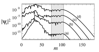
Figure 6: Outgoing boundary intensities are shown in momentum representation for sample eigenfunctions with $(a,b)=(0,1)$ in (a), $(a,b)=(-1,2)$ in (b), $(a,b)=(-2,3)$ in (c) and $(a,b)=(-3,4)$ in (d). The respective wavenumbers are $k\approx 73.32$ in (a), $k\approx 73.84$ in (b), $k\approx 74.06$ in (c) and $k\approx 74.17$ in (d). Successive examples have been scaled by arbitrary factors to separate them graphically. All of these examples have $F_{\rm min}=0$, $F_{\rm max}=1$ and similar values of $kR\approx 74$ and therefore share a common “allowed region” associated with the boundary-localised waves (49), occupying the band $kR<m<\sqrt{2}kR$ and indicated by the shaded region in the figure.

Figure 6 shows four examples of $\psi_{+}$-eigenfunctions for boundary condition (46), corresponding respectively to $(a,b)=(-3,4)$, $(-2,3)$ $(-1,2)$ and $(0,1)$. A prominent feature of all four examples is that, following decay from a peak around $m=33$ to the border at $m=kR\approx 74$ between open and closed modes, there follows a plateau extending significantly into the closed region $m>kR$. This feature is explained in [20, 21] in terms of waves localised near the boundary wherever $F(s)>0$. We now offer a brief summary of this explanation, borrowing from the discussions in [20, 21].

Consider first the case where $F>0$ is a constant and $kR\gg 1$. Then one can find quasimodes decaying exponentially into the interior (denoting $p=m/kR$ and $s=R\theta$) of the form

$$\psi(r,\theta)\simeq{\rm e}^{-kq(R-r)+{\rm i}m\theta}={\rm e}^{-kq(R-r)+{\rm i}kps},$$ (49)

satisfying the interior wave equation if $p^{2}=1+q^{2}$ and the boundary conditions if $q=F$. Note that such boundary-localised solutions occupy the closed subspace corresponding to $p^{2}>1$. If $F$ now varies, but over a scale longer than that of a wavelength, we should therefore expect localised solutions formed by deformations of these states, spread in momentum representation over the region

$$1+F_{\rm min}^{2}<p^{2}<1+F_{\rm max}^{2},$$

where

$$F_{\rm max} = {\rm max}({\rm max}(F(s)),0)$$

$$F_{\rm min} = {\rm max}({\rm min}(F(s)),0).$$

Exact eigenfunctions will then generically couple to such local solutions and lead to the plateau structures shown in Fig. 6. Heuristically we can interpret the observed plateaux as being the result of tunnelling in momentum space from the primary quasimode around $m=33$ to an “allowed region” $1+F_{\rm min}^{2}<p^{2}<1+F_{\rm max}^{2}$ introduced by the boundary-localised mode. In fact, the four examples in Fig. 6 were chosen to have the same values of $F_{\rm min}=0$ and $F_{\rm max}=1$, and one does indeed then observe that the plateaux occupy the same interval, indicated by the shaded strip in the figure.

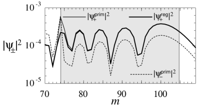
Figure 7: The outgoing boundary intensity $|\psi_{+}^{\rm reg}|^{2}$ defined by the regularised decomposition is shown as a heavy continuous curve over the plateau region for case (c) of Fig. 6: as in Fig. 6, the “allowed region” $1<p^{2}<F_{\rm max}^{2}$ is indicated by the shaded strip. Also shown, as a thin continuous curve, is the version $|\psi_{+}^{\rm prim}|^{2}$ obtained from the primitive decomposition. The thin dashed curve shows the primitive incoming intensity $|\psi_{-}^{\rm prim}|^{2}$. The primitive and regularised outgoing intensities differ significantly only near $m=kR\approx 74$, where the primitive case shows an expected divergence. The smaller, but significant, incoming intensity observed in the primitive case is qualitatively different from the regularised case, where the incoming intensity is zero or exponentially smaller than the outgoing intensity (depending on the conventions used to define the contour $\Gamma_{0}$ in Sec. 5.1).

This example offers a useful illustration of the most significant differences between the regularised and primitive decompositions — and their corresponding definitions of $\psi_{\pm}(s)$. In Fig. 7 we have selected the eigenfunction corresponding to case (c) of Fig. 6 and shown it (as the thick continuous curve) in more detail over its plateau region $1<p^{2}<F_{\rm max}^{2}$. Also shown are the primitive version (as a thin continuous curve) and the primitive incoming solution (as the thin dashed curve). As expected, the regularised and primitive outgoing intensities are very close, hardly distinguishable on this log plot, except that the primitive intensity becomes significantly larger in the region of critical incidence $p^{2}\approx 1$. We emphasise that this divergence is an artefact of the primitive decomposition, and its failure to deal properly with curvature at critical reflection, rather than an intrinsic characteristic of the solution itself.

The second difference is that, in the case of primitive decomposition, we obtain a smaller, but nonetheless significant, incoming component even in the “evanescent” region $p^{2}>1$, see Fig. 7. By contrast, the incoming component vanishes for the regularised decomposition. The nonvanishing primitively-defined incoming wave can be understood further by explicitly evaluating the shift operator for the primitive decomposition. Evaluating expression (28) for the special case of the circle yields a primitive shift operator represented by a diagonal matrix with entries

$$(\hat{S}^{\rm prim})_{mm}=\frac{\sqrt{1-m^{2}/z^{2}}J_{m}(z)-{\rm i}J_{m}^{\prime}(z)}{\sqrt{1-m^{2}/z^{2}}J_{m}(z)+{\rm i}J_{m}^{\prime}(z)};$$ (50)

which needs to be compared with $\hat{S}$ in (47) for the regularised decomposition. For closed components with $m^{2}>z^{2}\equiv(kR)^{2}$, and using the Debye approximation for the numerator, Eq. (50) vanishes at leading order. However, the next-to-leading order contributions do not cancel. Therefore $\psi_{-}^{\rm prim}=\hat{S}^{\rm prim}\psi_{+}^{\rm prim}$ does not vanish as does the regularly-defined incoming wave, or even decay exponentially as one would expect for properly-defined evanescent waves. Instead, it is only smaller than $\psi_{+}^{\rm prim}$ by a factor scaling algebraically with $1/k$. This failure of the primitive decomposition to separate evanescently incoming and outgoing solutions at all orders puts it at a significant disadvantage at describing such solutions compared to the regularised decomposition.

6.4 Husimi functions and Goos-Hänchen shifts

A particularly helpful means of presenting eigenmodes of this problem is by the boundary Husimi functions. Here we are guided by previous applications to dielectric problems [36, 37, 38, 39], where a definition of boundary Husimi functions has been proposed. This amounts in our language to applying the conventional definition of Husimi functions to the primitive in-out components

$$\Psi^{\rm prim}_{\pm}=\sqrt{\hat{P}}\psi_{\pm}$$ (51)

discussed further in B. In this paper we choose to work instead with a variation

$$\Psi_{\pm}=\hat{D}_{0}^{-1/2}\psi_{\pm}$$ (52)

in which $\hat{P}^{1/2}$ is replaced by its regularised analogue $\hat{D}_{0}^{-1/2}$. That is, we define

$$H_{\pm}(s_{0},p_{0})=|\langle{s_{0},p_{0}}|{\Psi_{\pm}}\rangle|^{2},$$

where the state $|{s_{0},p_{0}}\rangle$ corresponds to the boundary function

$$\langle{s}|{s_{0},p_{0}}\rangle=\sum_{n=-\infty}^{\infty}\left(\frac{k}{2\pi b^{2}}\right)^{1/4}{\rm e}^{-k(s-s_{0}-n\ell)^{2}/4b^{2}+{\rm i}kp_{0}(s-s_{0}-n\ell)}$$

and the inner product is

$$\langle{\Psi}|{\Phi}\rangle=\int_{0}^{\ell}\Psi^{*}(s)\Phi(s){\rm d}s.$$

Using (52) rather than (51) gives a Husimi function that is better behaved around the critical line $p^{2}=1$ but is otherwise very similar in the region $p^{2}<1$ and does not have a significant impact on the discussion following.

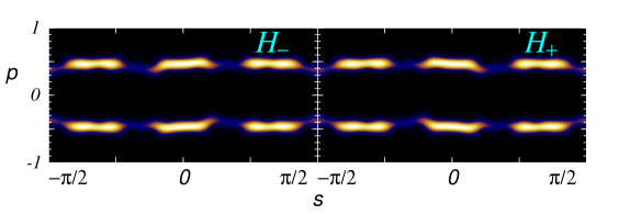
Figure 8: Boundary Husimi representations are shown of the outgoing and incoming solutions for the example labelled (d) in Fig. 6.

A particular pair of Husimi functions $H_{+}(s,p)$ and $H_{-}(s,p)$ calculated in this way is shown in Fig. 8, corresponding to the eigenmode labelled (d) in Fig. 6. The incoming and outgoing modes in the figure are qualitatively similar but display differences in detail that are explained by the application of the reflection operator in (48) — or equivalently by the Goos-Hänchen (GH) shift [22, 23, 24, 25, 32, 33]. Goos-Hänchen and related perturbations of ray dynamics are typically explained in terms of a shifting of the centre of a Gaussian or other localised beam following reflection from a boundary or interface. Such approaches provide a clear physical interpretation of the effect but seem unnatural in the context of calculating eigenfunctions, where no Gaussian beams appear in the rather more complicated wave patterns that one finds in typical cases. We now point out that the in-out decomposition of boundary solutions explored in this paper provide a much more direct way of describing the effect in this context. It makes it possible to explain the GH shift in terms of the tools that are naturally used to calculate eigenfunctions with chaotic or otherwise nonintegrable ray dynamics. Furthermore, the improved treatment of critical reflection such as provided by the regularised decomposition may allow improved descriptions of effects such as Fresnel filtering that are observed in associated parts of phase space, although we do not pursue that issue explicitly in this paper.

The incoming and outgoing solutions respectively satisfy the equations

$$\hat{r}\hat{S}\psi_{+}=\psi_{+}$$

and

$$\hat{S}\hat{r}\psi_{-}=\psi_{-},$$

where $\hat{S}$ describes the ray dynamics of specular reflection and is common to all cavity problems occupying the same domain, irrespective of boundary conditions. The GH shift may be incorporated simply by representing $\hat{r}$ in the exponential form (11) and regarding it as a quantisation of the flow of a Hamiltonian generator $h(s,p)$. The complete dynamics appropriate to $\psi_{\pm}$ are then obtained simply as a stroboscopic intertwining of this “Goos-Hänchen map” and the regular, specular ray dynamics — albeit in opposite orders for $\psi_{+}$ and $\psi-$.

The reflection operator in (48) is generated by

$$\hat{h}=\frac{{\rm i}}{k}\log\frac{1+{\rm i}\hat{X}}{1-{\rm i}\hat{X}}.$$

Away from the critical line $p^{2}=1$ this has the leading-order “primitive” symbol

$$h(s,p)=\frac{{\rm i}}{k}\log\frac{1+{\rm i}F(s)/\sqrt{1-p^{2}}}{1-{\rm i}F(s)/\sqrt{1-p^{2}}}=\frac{{\rm i}}{k}\log\frac{\sqrt{1-p^{2}}+{\rm i}F(s)}{\sqrt{1-p^{2}}-{\rm i}F(s)}$$

and the Goos-Hänchen map can be approximated at leading order by

$$\Delta s \approx {{\partial h}\over{\partial p}}=-\frac{2}{k}\frac{F(s)p/\sqrt{1-p^{2}}}{1-p^{2}+F(s)^{2}}$$

$$\Delta p \approx -{{\partial h}\over{\partial s}}=-\frac{2}{k}\frac{F^{\prime}(s)\sqrt{1-p^{2}}}{1-p^{2}+F(s)^{2}}.$$ (53)

Note that $\Delta s$ and $\Delta p$ are $O(1/k)$ and therefore act as perturbations of the usual specular ray dynamics. Note also that there is a nontrivial shift in momentum as well as position here because the local reflection phase depends on $s$. In the case of planar reflection, where the reflection phase is constant along the interface, the Goos-Hänchen map changes $s$ but not $p$, as prescribed in classical descriptions of the effect.

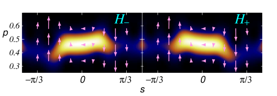
Figure 9: An expanded view is given of the middle-upper lobes of Fig. 8. Superimposed is the Hamiltonian vector field of the Goos-Hänchen map, defined explicitly by (6.4).

The breaking by the boundary conditions of integrability is strong enough in the example of Fig. 8 to localise the mode within an island chain of Goos-Hänchen-perturbed ray dynamics (see [23] for a treatment of this effect in the context of dielectric cavities). In Fig. 9 we illustrate the Goos-Hänchen vector field $(\Delta s,\Delta p)$ over part of phase space surrounding the point $(s,p)=(0,1/2)$, which lies at the centre of the middle-upper lobes of the Husimi functions of Fig. 8: this is where the incoming and outgoing Husimi functions differ most in this example. One sees that the vector field is indeed entirely consistent with the deformation of the incoming Husimi function relative to its outgoing equivalent: features lying at the bases of the Hamiltonian vectors for the former case lie at their tips in the latter case. Note that Poincaré plots of the corresponding dynamics (Goos-Hänchen map following the specular map in the outgoing case and preceding it in the incoming case) show a similar deformation (not shown).

7 Application to dielectric cavities

Our final application is to the problem of calculating resonant modes in dielectric cavities. The problem is solved explicitly here for the circular cavity with boundary conditions appropriate to TM polarisation. This simple problem can be solved analytically by elementary means: our aim, however, is to illustrate the application of the method to inside/outside problems in a way that it might later be generalised to less trivial, noncircular domains.

In this case, we must separately solve two wave problems; the interior one whose solution and normal derivative we denote as usual by $\psi$ and $\mu$ respectively, and which is such that

$$-\nabla^{2}\psi=n^{2}k^{2}\psi,\qquad{\bf x}\in\Omega,$$

and the exterior problem whose solution and normal derivative are respectively denoted by $\varphi$ and $\nu$ and for which

$$-\nabla^{2}\varphi=k^{2}\varphi,\qquad\quad{\bf x}\in\Omega^{\prime}.$$

Here the refractive index inside the cavity is $n>1$ while outside we set $n=1$. Following the discussion of Sec. 5.2, the interior and exterior problems separately define decompositions $\psi=\psi_{-}+\psi_{+}$ and $\varphi=\varphi_{-}+\varphi_{-}$ and shift operators such that

$$\psi_{-}=\hat{S}^{\rm int}\psi_{+}$$

and

$$\varphi_{-}=\hat{S}^{\rm ext}\varphi_{+}.$$

The shift operators $\hat{S}^{\rm int}$ and $\hat{S}^{\rm ext}$ differ by using Green functions corresponding to different values of the refractive index and by the boundary integral equation for the exterior problem having a unit normal pointing into rather than out of the domain concerned, (see Eqn. (38)). According to the conventions suggested in Sec. 5.2, where the endpoint contour $\Gamma_{0}$ is chosen for closed modes to account for all of the boundary integral, we find that the external shift operator vanishes,

$$\hat{S}^{\rm ext}=0$$

and Eqn. (40) holds (see C for discussion of alternative conventions). Of course it is the field $\varphi({\bf x})$ in the exterior ${\bf x}\in\Omega^{\prime}$ that is physically observed here: see D for a discussion of the determination of the full solution, inside and outside the cavity, from its restriction to the boundary.

The end result will be presented more compactly if we use the shift operator for the external problem to define a Dirichlet-to-Neumann map $\hat{F}$, such that

$$\nu=k\hat{F}\varphi.$$ (54)

In general (after some manipulation),

$$\hat{F}={\rm i}\left(\hat{D}_{0}^{\rm ext}\right)^{-1}\left(\hat{I}+{\rm i}\hat{D}_{1}^{\rm ext}\right).$$ (55)

and we note that $\hat{F}$ itself is independent of conventions used in the in-out decomposition. Note also that $\hat{F}$ is determined by the condition of having no incoming waves at infinity and is independent of boundary conditions on the cavity itself.

We next apply the cavity’s boundary conditions. To be concrete, we impose TM boundary conditions

$$\psi(s)=\varphi(s)\qquad\mbox{and}\qquad\mu(s)=\nu(s),$$

but emphasise that the following discussion generalises easily. Together with (54), this provides a boundary condition formally very much like that of Sec. 6 and leads to a similar-looking reflection operator

$$\hat{r}=\frac{1+{\rm i}\hat{X}}{1-{\rm i}\hat{X}},$$

except that, in this case,

$$\hat{X}=\hat{D}^{\rm int}_{1}+\frac{1}{n}\hat{D}^{\rm int}_{0}\hat{F}.$$

Note that this reflection operator can alternatively be written

$$\hat{r}=\left(n(\hat{D}_{0}^{\rm int})^{-1}(\hat{I}-{\rm i}\hat{D}_{1}^{\rm int})-{\rm i}\hat{F}\right)^{-1}\left(n(\hat{D}_{0}^{\rm int})^{-1}(\hat{I}+{\rm i}\hat{D}_{1}^{\rm int})+{\rm i}\hat{F}\right).$$ (56)

This allows for a more direct comparison with classical expressions for the corresponding Fresnel reflection coefficient

$$r=\frac{n\cos\alpha-\cos\beta}{n\cos\alpha+\cos\beta}.$$

This comparison is achieved on making the identifications

$$(\hat{D}_{0}^{\rm int})^{-1}(\hat{I}-{\rm i}\hat{D}_{1}^{\rm int})\approx(\hat{D}_{0}^{\rm int})^{-1}(\hat{I}+{\rm i}\hat{D}_{1}^{\rm int})\sim\cos\alpha\equiv\sqrt{1-p^{2}}$$

and

$$-{\rm i}\hat{F}=(\hat{D}_{0}^{\rm ext})^{-1}(\hat{I}+{\rm i}\hat{D}_{1}^{\rm ext})\sim\cos\beta\equiv{\rm i}\sqrt{n^{2}p^{2}-1}$$

appropriate to the ray-dynamical limit, where $\alpha$ and $\beta$ are respectively the angles of incidence and refraction of a ray hitting the boundary from inside.

We can now determine resonant modes as solutions of the secular condition

$$\psi_{+}=\hat{r}\hat{S}^{\rm int}\psi_{+}.$$ (57)

This is once again formally much as in the model example of Sec. 6. The main qualitative difference is that, whereas the restriction of the reflection operator to the open subspace has eigenvalues on the unit circle in the example of Sec. 6, here the relevant eigenvalues of $\hat{r}$ lie inside the unit circle. reflecting the lossiness of the system (to radiation to infinity). As a consequence, the solutions of the secular equation are obtained here for complex values of $k$, as should be expected for resonant modes with a finite lifetime.

We point out that composing the shift operator $\hat{S}$ with a subunitary reflection operator $\hat{r}$ as in (57) provides a very natural wave analogue of the ray-dynamical approach taken, for example, in [40, 41, 42, 43]. There, emission from dielectric cavities is treated by iterating initial densities of rays under a composition of the ray-dynamical analogues of $\hat{S}$ and $\hat{r}$, namely a Perron-Frobenius operator encoding the Poincaré-Birkhoff map of the internal dynamics and a transmission loss determined from classical Fresnel coefficients. The combined operator in (57) simply replaces each of those elements by a corresponding wave map. It therefore offers a basis for treating inherently wave effects within the broader approach of [40, 41, 42, 43], particularly, for example, the more complicated transmission losses encountered around the critical lines (see also further discussion below).

We now specialise these results to the case of a circular cavity. One then finds from (55) that $\hat{F}$ is diagonal and has elements

$$(\hat{F})_{mm}=\frac{H_{m}^{\prime}(kR)}{H_{m}(kR)}.$$

(Of course this can also be deduced directly from (54) by elementary means but our aim here is to offer a discussion that generalises.) We also find that

$$\left((\hat{D}_{0}^{\rm int})^{-1}(\hat{I}+{\rm i}\hat{D}_{1}^{\rm int})\right)_{mm}=-{\rm i}\frac{H_{m}^{\prime}(nkR)}{H_{m}(nkR)}$$

(for all $m$) and

$$\left((\hat{D}_{0}^{\rm int})^{-1}(\hat{I}-{\rm i}\hat{D}_{1}^{\rm int})\right)_{mm}=\cases{{\rm i}\frac{{H^{*}_{m}}^{\prime}(nkR)}{H^{*}_{m}(nkR)},&if $|m|\leq nkR$\\ {\rm i}\frac{J_{m}^{\prime}(nkR)}{J_{m}(nkR)},&if $|m|>nkR$,}$$

from which the reflection operator follows by (56). Note that this provides a means of calculating curvature corrections to Fresnel laws, such as described in [44], while also incorporating the phase information relevant to, for example, Goos-Hänchen shifts.

The elements $(\hat{F})_{mm}$ undergo a transition across the critical lines of the exterior problem, defined by $|m|=kR$. They are approximately imaginary for $|m|<kR$ and define through (56) diagonal elements of the reflection operator such that $|(\hat{r})_{mm}|<1$: corresponding resonant modes leak directly by refraction to the exterior and are short-lived. Whispering gallery modes lie within the open subspace of the interior problem, for which $|m|<nkR$, and the closed subspace of the exterior problem, for which $|m|>kR$. The corresponding elements

$$(\hat{F})_{mm}=\frac{Y_{m}^{\prime}(kR)-{\rm i}J_{m}^{\prime}(kR)}{Y_{m}(kR)-{\rm i}J_{m}(kR)}\approx\frac{Y_{m}^{\prime}(kR)}{Y_{m}(kR)}+{\rm i}\frac{2}{\pi kR}\frac{1}{Y_{m}(kR)^{2}}$$

of $\hat{F}$ are approximately real but retain small positive imaginary parts and lead to diagonal elements of $\hat{r}$ which are close to, but slightly less than, unity in magnitude: the corresponding whispering gallery modes therefore have a long but finite lifetime.

A representation of $\hat{r}$ in exponential form (11) defines a generator $\hat{h}$ with significant nonHermitian components in the region $|m|<kR$ and smaller but nonvanishing nonHermitian components over $kR<|m|<nkR$, reflecting the lossiness of the system as a whole. Away from the critical lines $|m|=kR$, where the reflection phase is not rapidly varying, we may approximate this operator straightforwardly by a Goos-Hänchen map for which the Hamiltonian generator $h(s,p)$ has imaginary components and is obtained as the ray-dynamical symbol of $\hat{h}={\rm i}\log(\hat{r})/k$. Across the critical lines $|m|=kR$, where the reflection phase is rapidly varying, the ray-dynamical shifts corresponding to $\hat{r}$ are less easy to work out. However, one can still formally use $\hat{r}$ to define a ray-dynamical map — it is just not as close to the identity map and its generator is not as easily approximated. Further investigation of this issue will hopefully lead to a better understanding of the modifications necessary to incorporate by Goos-Hänchen and related effects into a ray dynamics around the physically important regime of critical refraction.

In summary, we have shown how the in-out decompositions discussed in this paper lead naturally to expected results for resonant modes of a dielectric circle. We emphasise, however, that the general approach extends to deformed cavities. In particular, we demonstrate that this approach shows promise for a better understanding of effects such as Goos-Hänchen and similarly modified dynamics near critical lines; in the interests of brevity we do not pursue this issue any further in this paper.

8 Conclusions

We have proposed an approach for separating the boundary solutions of cavity problems into incoming and outgoing components that allows boundary integral equations to be recast as transfer-operator equations. The resulting “shift operator” maps the outgoing component leaving the boundary onto the incoming component arriving back at the boundary having crossed the cavity’s interior. The shift operator is completely independent of the boundary conditions and decouples from them the problem of wave propagation through the interior. The boundary conditions are used separately to complete the problem by defining a reflection operator mapping the component arriving at the boundary to the reflected, outgoing component leaving it again towards the interior.

The underlying intuition behind this approach is familiar in the context of semiclassical approximations [1]. We believe, however, that using (8) and (9) rather than ray-based ideas in order to define the in-out decomposition of the boundary solution provides an ideal platform on which to extend these ideas beyond leading-order approximations. We hope that the exactly defined shift operator will enable the efficient treatment of diffraction and tunnelling effects, for example. The approach also holds promise for more complex problems where small subsystems demanding fully wave-based analysis may coexist with larger structures necessitating ray-based approximations [16, 15]. In that context, the ability to perform fully wave-based calculations within a formalism that is suitable also for large-scale ray approximations will allow their efficient integration within hybrid methods.

Equations (8) and (9) lie at the heart of everything calculated in this paper. Their key advantage is in allowing a very natural in-out decomposition to be made while owing nothing to semiclassical approximation. There remains a significant degree of freedom, however, in choosing the singular parts of the Green operators used to construct the outgoing component. The simplest “primitive” choice set out in Sec. 4 appears very natural from the standpoint of ray-based calculations and gives the right leading-order behaviour straightforwardly (see B). It is singular, however, around criticially incident waves arriving tangentially at the boundary and fails to define appropriately decaying outgoing components in evanescent regimes (see Fig. 7 and the surrounding discussion in Sec. 6.3). We have therefore suggested in Sec. 5 a second approach appropriate to domains with analytic boundaries. Here, we have used asymptotic analysis of the boundary integrals to motivate a decomposition based on integration contours on the complexified boundary. This approach is at once able to provide semiclassical approximation beyond all orders and amenable to exact analysis. It has been shown to work well in providing a solution of model problems with circular geometry in Secs. 6 and 7.

Three outstanding problems remain which deserve further investigation. First, the applications so far carried out have been to the special case of a circular domain for which the shift operator can be fully determined analytically. The regular decomposition is also applicable to more general (analytic) domains, but will require some numerical intervention in such cases to implement fully. Efficient means of performing steps such as the operator inversions in (35) therefore need attention, as do practical approaches to truncation of the complex contours in the presence of chord-length singularities expected for generic boundaries. Second, while we hope that equations (8) and (9) will eventually provide a basis also for the treatment of nonconvex domains, or boundaries with corners, these will respectively require more careful analysis of the nontrivial operator inversion on the right hand side of (36) and the isolation of the singular parts of boundary integrals at corners. Third, there remains some degree of “ugliness” in the treatment of the transition from open to closed modes in the discussion provided for the regularised decomposition. Although the regularised components do not diverge around criticality as do their primitive counterparts, they do still undergo a discontinuous change. This is due to a coalescence and switching of identities of incoming and outgoing components around critical reflection and may therefore be unavoidable, but one would ideally manage the transition in a smoother way.

Appendix A Green operator on a line

The extraction of the singular part $\hat{G}_{0}^{\rm sing}$ of the Green operator plays a central role in the decomposition of the boundary functions on which we base the transfer-operator representation of the boundary integral equations. In the case of the primitive decomposition described in Sec. 4, we have defined $\hat{G}_{0}^{\rm sing}$ so that it corresponds to replacing the boundary locally by a straight line. This allows the simple, compact representation given in (20), which is derived in this appendix.

Let $\hat{G}_{0}^{\rm sing}$ be defined by (19). Before taking the limit $\varepsilon\to 0$ in this definition, the operator takes the form of a convolution of the test function $\mu(s)$ with a function whose Fourier transform is

$$\tilde{G}_{0}^{\rm sing}(p) = \frac{{\rm i}}{4}\int_{-\infty}^{\infty}\rme^{-{\rm i}kps}H_{0}^{(1)}(k\sqrt{s^{2}+\varepsilon^{2}})\rmd s$$ (58)

$$= \cases{\frac{{\rm i}}{2k\sqrt{1-p^{2}}}\rme^{{\rm i}k\varepsilon\sqrt{1-p^{2}}}&if $p^{2}<1$\\ \frac{1}{2k\sqrt{p^{2}-1}}\rme^{-k\varepsilon\sqrt{p^{2}-1}}&if $p^{2}>1$,}$$

where the latter form is tabulated in section 6.677 of [45]. Taking the limit $\varepsilon\to 0$, the action of $\hat{G}_{0}^{\rm sing}$ on the Fourier transform $\chi(p)$ of $\mu(p)$ is such that

$$\hat{G}_{0}^{\rm sing}\chi(p)=\chi(p)\times\cases{\frac{{\rm i}}{2k\sqrt{1-p^{2}}}&if $p^{2}<1$\\ \frac{1}{2k\sqrt{p^{2}-1}}&if $p^{2}>1$.}$$

This justifies the formal definition (20) of the singular part of the Green function, along with the integral version given in (23). The branches of the square root obtained for $p^{2}>1$ also explain the route of the contour in (23) around the branch points $p^{2}=1$.

We now derive the equivalent expression (24) for $\hat{G}_{1}^{\rm sing}$, beginning with its formal definition

$$\hat{G}_{1}^{\rm sing}\psi(s)=\lim_{\varepsilon\to 0}\frac{{\rm i}k}{4}\int_{-\infty}^{\infty}\frac{\varepsilon H_{0}^{\prime}\left(k\sqrt{|s-s^{\prime}|^{2}+\varepsilon^{2}}\right)}{\sqrt{(s-s^{\prime})^{2}+\varepsilon^{2}}}\psi(s^{\prime}){\rm d}s^{\prime}$$

analogous to (19). Note that applying this operator amounts taking a derivative with respect to $\varepsilon$ in (19) before taking the limit. Therefore, its action on the Fourier transform $\varphi(p)$ of $\psi(s)$ is obtained by multiplying it by the derivative

$$\tilde{G}_{1}^{\rm sing}(p) = \cases{-\frac{1}{2}\rme^{{\rm i}k\varepsilon\sqrt{1-p^{2}}}&if $p^{2}<1$\\ -\frac{1}{2}\rme^{-k\varepsilon\sqrt{p^{2}-1}}&if $p^{2}>1$,}$$ (59)

of (58) and then letting $\varepsilon\to 0$, after which

$$\hat{G}_{1}^{\rm sing}\varphi(p)=-\frac{1}{2}\varphi(p),$$

which demonstrates (24).

Appendix B Semiclassical approximation of the primitive decomposition

In this appendix we describe more explicitly some of the semiclassical results claimed in the main text for the primitive approximation.

Figure 10: The notation used for chord length and incidence angles is illustrated for the convex case.

To describe the primitive decomposition semiclassically, we begin with the following rewriting of (25)

$$\hat{S}_{0}=-2{\rm i}k\hat{G}_{0}\hat{P}-\hat{I}.$$

We next note that applying the operator $\hat{P}$ to a propagating boundary function of WKB form with local tangential momentum $p=\sin\alpha$ amounts at leading order to multiplication by $|\cos\alpha|$. Here $\alpha$ denotes the angle of incidence of the associated ray, defined with respect to a normal pointing into the domain $\Omega$ and we note that real chords on convex billiards satisfy $\cos\alpha>0$. Away from the diagonal $s=s^{\prime}$, where the singular contribution from $\hat{I}$ can be neglected, the Green function can be approximated by

$$G_{0}(s,s^{\prime};k)\simeq\frac{{\rm i}}{2k}\sqrt{\frac{k}{2\pi{\rm i}}\frac{1}{\cos\alpha}{{\partial^{2}L}\over{\partial\mathstrut{s}\partial\mathstrut{s^{\prime}}}}\frac{1}{\cos\alpha^{\prime}}}\;{\rm e}^{{\rm i}kL(s,s^{\prime})}.$$

For convex cavities, we find then that $\hat{S}_{0}$ can be represented at leading order by the kernel

$$S_{0}(s,s^{\prime})\simeq\sqrt{\frac{k}{2\pi{\rm i}}\frac{1}{\cos\alpha}{{\partial^{2}L}\over{\partial\mathstrut{s}\partial\mathstrut{s^{\prime}}}}\cos\alpha^{\prime}}\;{\rm e}^{{\rm i}kL(s,s^{\prime})},$$ (60)

where $\alpha$ and $\alpha^{\prime}$ are the chord’s angles of incidence defined in Fig. 10. One easily finds on using $\partial{L}/\partial{n^{\prime}}=\cos\alpha^{\prime}$ that a corresponding calculation of the kernel $S_{1}(s,s^{\prime})$ for $\hat{S}_{1}$ gives the same leading form. This justifies (29) for real rays in convex domains.

The situation is different, however, for nonconvex domains or for closed or evanescent modes represented by complex rays. Consider first the case of real rays in nonconvex domains. In this case one encounters ”ghost orbits” which pass through the exterior of $\Omega$ on the way from $s^{\prime}$ to $s$. In particular, chords which immediately leave $s^{\prime}$ towards the exterior will be such that $\partial{L}/\partial{n^{\prime}}=\cos\alpha^{\prime}<1$, in which case the kernels of $\hat{S}_{0}$ and $\hat{S}_{1}$ have opposite sign at leading order:

$$S_{0}(s,s^{\prime})\approx-S_{1}(s,s^{\prime}).$$ (61)

Note that ghost orbits can be shown to cancel systematically to all orders in the full secular equation [7], but their presence significantly complicates the present analysis by preventing a simple evaluation of the operator inversion in (28). More generally they prevent us from imposing (35) in a simple way. This is not surprising as we expect the corresponding external problem, discussed at the end of Sec. 5.2, to have nontrivial incoming components in nonconvex problems.

We state without proof that complex chords corresponding to evanescent wave propagation beyond criticality also satisfy (61). This is reflected also in the vanishing of the right hand side of (50) at leading order when $m^{2}>(kR)^{2}$. The result is that $\psi_{-}=\hat{S}\psi_{+}$ is in general smaller than $\psi_{+}$ in the closed region of momentum representation, although, as evidenced by Fig. 7, not exponentially so as the cancellation of the right hand side of (28) only occurs at leading order and nontrivial higher-order contributions remain.

We remark finally that a more explicit comparison with standard representations of the transfer operator can be made if the incoming and outgoing boundary waves are represented by $\Psi_{\pm}$ defined in (51) instead of $\psi_{\pm}$ and, replacing (25) and (26), correspondingly. The transformed shift operators $\hat{\cal S}_{0}$ and $\hat{\cal S}_{1}$ are then defined by

$$\hat{G}_{0}=\frac{{\rm i}}{2k}\frac{1}{\sqrt{\hat{P}}}\left(\hat{I}+\hat{\cal S}_{0}\right)\frac{1}{\sqrt{\hat{P}}}$$ (62)

and

$$\hat{G}_{1}=-\frac{1}{2}\frac{1}{\sqrt{\hat{P}}}\left(\hat{I}+\hat{\cal S}_{1}\right)\sqrt{\hat{P}}.$$ (63)

The direct analogue of (28) now yields a shift operator $\hat{\cal S}=\hat{P}^{1/2}\hat{S}\hat{P}^{-1/2}$ such that $\Psi_{-}=\hat{\cal S}\Psi_{+}$, and which can be represented by a kernel whose leading semiclassical approximation takes the standard form

$${\cal S}(s,s^{\prime})\simeq{\cal S}_{0}(s,s^{\prime})\simeq{\cal S}_{1}(s,s^{\prime})\simeq\sqrt{\frac{k}{2\pi{\rm i}}{{\partial^{2}L}\over{\partial\mathstrut{s}\partial\mathstrut{s^{\prime}}}}}\;{\rm e}^{{\rm i}kL(s,s^{\prime})},$$

given in [1].

Appendix C Alternative treatment of evanescent components

The treatment of evanescent components within the regularised decomposition has been described primarily in this paper while assuming that the endpoint contour component $\Gamma_{0}$ has been chosen to pass to the right of the saddle in Fig. 5(b). This has the advantage of simplifying the presentation of formal results by allowing, for example, condition (35) to hold at leading order semiclassically over both the open and closed subspaces.

Figure 11: The decomposition of contours illustrated here provides an alternative to the convention in Fig 5(b).

This is not the only possible choice of $\Gamma_{0}$, however. As described in Sec. 5, the saddle-point contribution to (31) undergoes a Stokes transition around real values of $p^{2}>1$ so that it is a priori equally valid for $\Gamma_{0}$ to pass to the other side of the saddle, as shown schematically in Fig 11. Choosing this alternative route provides us with different forms for $\hat{G}_{0,1}^{\rm sing}$ and $\hat{G}_{0,1}^{\rm reg}$ on the closed subspace, which we describe in this section for the case of the circle: note that, because $\Gamma_{1}$ is now nonempty, the corresponding components of $\hat{G}_{0,1}^{\rm reg}$ are nonzero. We emphasise that, throughout this appendix, the restrictions of $\hat{G}_{0,1}^{\rm sing}$ and $\hat{G}_{0,1}^{\rm reg}$ to the open subspace are unaffected by this choice.

We find for this alternative contour decomposition that

$$\left(\hat{G}_{0}^{\rm sing}\right)_{mm}=\frac{{\rm i}}{2k}\left({\rm i}\pi zY_{m}(z)J_{m}(z)-\pi zJ_{m}(z)^{2}\right)$$

and

$$\left(\hat{G}_{0}^{\rm reg}\right)_{mm}=\frac{{\rm i}}{2k}\left(2\pi zJ_{m}(z)^{2}\right)$$

in the case of the circle, while

$$\left(\hat{G}_{1}^{\rm sing}\right)_{mm}=-\frac{1}{2}\left(\pi zY_{m}(z)J_{m}(z)+\pi{\rm i}zJ_{m}^{\prime}(z)J_{m}(z)\right)$$

and

$$\left(\hat{G}_{1}^{\rm reg}\right)_{mm}=-\frac{1}{2}\left(-2\pi{\rm i}zJ_{m}^{\prime}(z)J_{m}(z)\right)$$

(all for $|m|>z$). This means in particular that condition (35), does not automatically hold in this convention, since

$$(\hat{S}_{0})_{mm}\equiv\left(\hat{G}_{0}^{\rm reg}\left(\hat{G}_{0}^{\rm sing}\right)^{-1}\right)_{mm}=\frac{2J_{m}(z)}{{\rm i}Y_{m}(z)-J_{m}(z)},$$

while

$$(\hat{S}_{1})_{mm}\equiv\left(\hat{G}_{1}^{\rm reg}\left(\hat{G}_{1}^{\rm sing}\right)^{-1}\right)_{mm}=\frac{2J_{m}^{\prime}(z)}{{\rm i}Y_{m}^{\prime}(z)-J_{m}^{\prime}(z)}$$

(again, all for $|m|>z$). However, we do still find that considerable simplification occurs in the shift operator itself, because the closed components now satisfy

$$\left(\hat{G}_{1}^{\rm reg}-\hat{G}_{0}^{\rm reg}\left(\hat{G}_{0}^{\rm sing}\right)^{-1}\hat{G}_{1}^{\rm sing}\right)_{mm}=\left(\hat{G}_{0}^{\rm reg}\left(\hat{G}_{0}^{\rm sing}\right)^{-1}\right)_{mm}$$ (64)

(this identity is not immediately obvious but follows from manipulation of the forms given above for $\hat{G}_{0,1}^{\rm sing}$ and $\hat{G}_{0,1}^{\rm reg}$ and use of the Wronskian identities for Bessel functions). In particular, we find from (36) that the shift operator of the interior problem still vanishes identically for closed modes $|m|>z$:

$$\hat{S}^{\rm int}=0.$$

The solution of the interior problem is then not qualitatively changed by adopting this alternative convention and we simply find that, beyond leading order, the construction of the shift operator is complicated somewhat in the closed subspace.

On the other hand, the shift operator for the exterior problem is changed qualitatively. According to (39), the closed components of this operator then satisfy

$$(\hat{S}^{\rm ext})_{mm}=(\hat{S}_{0})_{mm}=\frac{2J_{m}(z)}{{\rm i}Y_{m}(z)-J_{m}(z)},$$

so that, although the external shift operator is exponentially small ($J_{m}(z)\ll Y_{m}(x)$ in the evanescent regime), it does not vanish. A convention in which the shift operator for the exterior problem is exponentially small but nonvanishing may be an attractive way of treating tunnelling effects directly. For convex domains, waves leaving the boundary evanescently towards the exterior may encounter, and be reflected at, caustics some distance from the boundary before returning to it. In the circular case such caustics are encountered at a radius $kr=|m|>kR$ where the outgoing Hankel function undergoes a Stokes transition. In the language of ray asymptotics, although a real ray leaving the boundary never returns, a contributing complex ray may (see [34] for an explicit discussion of such exterior complex rays in the context of tunnelling emission from dielectric cavities). In the convention used in the main text, such returning evanescent waves are simply included in $\varphi_{+}$. The alternative here allows such returning evanescent waves to contribute to a nonvanishing component $\varphi_{-}$ and to be treated separately.

One final comment is that yet another convention is obtained by defining $\hat{G}_{0,1}^{\rm sing}$ as a weighted mean of the singular parts defined in this appendix and those used in the main text. Although space does not allow us to present details here, it is found that (64) still holds in such conventions, as do the identities $(\hat{S}^{\rm int})_{mm}=0$ and $(\hat{S}^{\rm ext})_{mm}=(\hat{S}_{0})_{mm}$. Furthermore, a symmetrically-weighted mean leads, for example, to operators $\hat{D}_{0}$ and $\hat{D}_{1}$ having purely imaginary components in the closed subspace.

Appendix D Mapping boundary solutions to the interior

In this appendix we summarise how the solution inside the domain can be determined in terms of the in-out boundary solutions. Let

$$(\hat{\cal G}_{0}\mu)({\bf x}) = \int_{\partial\Omega}G_{0}({\bf x},s^{\prime};k)\mu(s^{\prime}){\rm d}s^{\prime}$$ (65)

$$(\hat{\cal G}_{1}\psi)({\bf x}) = \int_{\partial\Omega}{{\partial G_{0}({\bf x},s^{\prime};k)}\over{\partial n^{\prime}}}\psi(s^{\prime}){\rm d}s^{\prime}$$ (66)

extend the Green operators defined by (3) and (4) so that they map boundary functions to functions defined on the interior $\Omega$. Then the interior solution $\psi({\bf x})$ can be written formally

$$\psi({\bf x})=\hat{\cal G}_{0}\mu-\hat{\cal G}_{1}\psi.$$

Written in terms of the in-out components, this becomes (after some manipulation)

$$\psi({\bf x})=\left({\rm i}k\hat{\cal G}_{0}\hat{D}_{0}^{-1}(\hat{I}+{\rm i}\hat{D}_{1})-\hat{\cal G}_{1}\right)\psi_{-}-\left({\rm i}k\hat{\cal G}_{0}\hat{D}_{0}^{-1}(\hat{I}-{\rm i}\hat{D}_{1})+\hat{\cal G}_{1}\right)\psi_{+}.$$

If the extended Green operators satisfy the following generalisation of condition (35)

$$\hat{\cal G}_{0}\left(\hat{G}_{0}^{\rm sing}\right)^{-1}=\hat{\cal G}_{1}\left(\hat{G}_{1}^{\rm sing}\right)^{-1},$$ (67)

then the contribution from $\psi_{-}$ drops out of this equation after using the relations (41), (42) and the interior solution is given by the simplified expression

$$\psi({\bf x})=-2{\rm i}k\hat{\cal G}_{0}\hat{D}_{0}^{-1}\psi_{+}.$$

Condition (67) holds at leading order semiclassically for all of the decompositions examined in this paper and can be shown to hold exactly in the case of the circle. How accurately it holds for more general domains is a topic of investigation but it certainly forms an appropriate starting point for semiclassical approximation.

Figure 12: The notation used in equation (68) is illustrated.

Within semiclassical approximation one may therefore write

$$\psi({\bf x})=\int_{\partial\Omega}{\cal T}({\bf x},s^{\prime})\psi_{+}(s^{\prime}){\rm d}s^{\prime},$$

where

$${\cal T}({\bf x},s^{\prime})\simeq-2{\rm i}kG_{0}({\bf x},s^{\prime};k)\cos\alpha^{\prime}$$

and $\alpha^{\prime}$ is the angle at which the line from $s^{\prime}$ to ${\bf x}$ leaves the boundary. If we place ${\bf x}$ on a section parametrised by arclength $s$ and such that the line from $s^{\prime}$ arrives with incidence angle $\alpha$, this can be approximated more explicitly by the form

$${\cal T}({\bf x},s^{\prime})\simeq\sqrt{\frac{k}{2\pi{\rm i}}\frac{1}{\cos\alpha}{{\partial^{2}L}\over{\partial\mathstrut{s}\partial\mathstrut{s^{\prime}}}}\cos\alpha^{\prime}}\;{\rm e}^{{\rm i}kL({\bf x},s^{\prime})},$$ (68)

generalising (60). We note finally that an analogous boundary integral provides the solution $\varphi({\bf x})$ of the exterior problem in terms of the component $\varphi_{+}(s)$ leaving the boundary towards infinity, except that the angles of incidence are defined relative to the outward pointing normal in that case: in the dielectric problem, $\alpha^{\prime}$ is replaced by the angle of refraction $\beta^{\prime}$.

References

References

- [1] Bogomolny E 1992 Nonlinearity 5 85
- [2] Boasman P A 1994 Nonlinearity 7 485
- [3] Georgeot B and Prange R E 1995 Phys. Rev. Lett. 74(15) 2851–2854
- [4] Georgeot B and Prange R E 1995 Phys. Rev. Lett. 74(21) 4110–4113
- [5] Harayama T and Shudo A 1992 Phys. Lett. A 165 417
- [6] Tasaki S, Harayama T and Shudo A 1997 Phys. Rev. E 56 R13
- [7] Harayama T, Shudo A and Tasaki S 1999 Nonlinearity 12 1113–1149
- [8] Sieber M, Primack H, Smilansky U, Ussishkin I and Schanz H 1995 Journal of Physics A: Mathematical and General 28 5041
- [9] Sieber M 1998 Nonlinearity 11 1607
- [10] Blümel R, Antonsen T, Georgeot B, Ott E and Prange R 1996 Phys. Rev. E 53 3284–3302
- [11] Blümel R, Antonsen T, Georgeot B, Ott E and Prange R 1996 Phys. Rev. Letters 76 2476–2479
- [12] Tanner G and Sondergaard N 2007 J. Phys. A 40 R443
- [13] Hemmady S, Jr T M A, Ott E and Anlage S M 2012 IEEE Trans. Electromagnetic Compatibility 54 758
- [14] Tanner G 2009 J Sound Vibr 320 1023
- [15] Chappell D J, Tanner G, Löchel D and Sondergaard N 2013 Proc Roy Soc A 469 2155 20130153
- [16] Maksimov D N and Tanner G 2011 J Acoust Soc Am 130 1337
- [17] Gnutzmann S and Smilansky U 2006 Advances in Physics 55 527–625
- [18] Kuchment P 2008 Proc. Sympos. Pure Math. Amer. Math. Soc. 77 291–312
- [19] Hamdin H B 2012 Boundary element and transfer operator methods for multi-component wave systems Ph.D. thesis University of Nottingham
- [20] Berry M V and Dennis M R 2008 J. Phys. A 41 135203
- [21] Bogomolny E, Dennis M R and Dubertrand R 2009 J. Phys. A 42 335102
- [22] Schomerus H and Hentschel M 2006 Phys. Rev. Lett. 96 243903
- [23] Unterhinninghofen J, Wiersig J and Hentschel M 2008 Phys. Rev. E 78 016201
- [24] Altmann E G, Magno G D and Hentschel M 2008 Euro. Phys. Lett. 84 10008
- [25] Unterhinninghoffen J and Wiersig J 2010 Phys. Rev. Lett. 82 026202
- [26] Doron E and Smilansky U 1992 Nonlinearity 5 1055–1084
- [27] Rouvinez C and Smilansky U 1995 J. Phys. A 28 77–103
- [28] Schanz H and Smilansky U 1995 Chaos, Solitons and Fractals 5 1289–1309
- [29] Prosen T 1994 J. Phys. A:Math. Gen. 27 L709–L714
- [30] Prosen T 1995 J. Phys. A: Math. Gen. 28 4133–4155
- [31] Prosen T 1996 Physica D 91 244–277
- [32] Gorodetsky M L and Fomin A E 2006 IEEE Journal of Selected Topics in Quantum Electronics 12 33
- [33] Gorodetsky M L and Fomin A E 2007 Quantum Electronics 37 167
- [34] Creagh S C and White M M 2010 J. Phys. A 43 465102
- [35] Abramowitz M and Stegun I A 1972 Handbook of Mathematical Functions (New York: Dover)
- [36] Nöckel J U and Stone A D 1997 Nature 385 45
- [37] Bäcker A, Fürstberger S and Schubert R 2004 Phys. Rev. E 70 036204
- [38] Hentschel M, Schomerus H and Schubert R 2003 Europhys. Lett. 62 636
- [39] Wiersig J and Hentschel M 2008 Phys. Rev. Lett. 100 033901
- [40] Lee S Y, Rim S, Ryu J W, Kwon T Y, Choi M and Kim C M 2004 Phys. Rev. Lett. 93 164102
- [41] Lee S Y, Ryu J W, Kwon T Y, Rim S and Kim C M 2005 Phys. Rev. A 72 061801
- [42] Ryu J W, Lee S Y, Kim C M and Park Y J 2006 Phys. Rev. E 73 036207
- [43] Shinohara S and Harayama T 2007 Phys. Rev. E 72 036216
- [44] Hentschel M and Schomerus H 2002 Phys. Rev. E 65 045603
- [45] Gradshteyn I, Ryzhik I and Jeffrey A 1994 Table of integrals, series, and products 5th ed (Academic Press)