Fast and precise way to calculate the posterior for the local non-Gaussianity parameter $f_{\text{nl}}$ from cosmic microwave background observations

Abstract

We present an approximate calculation of the full Bayesian posterior probability distribution for the local non-Gaussianity parameter $f_{\text{nl}}$ from observations of cosmic microwave background anisotropies within the framework of information field theory. The approximation that we introduce allows us to dispense with numerically expensive sampling techniques. We use a novel posterior validation method (DIP test) in cosmology to test the precision of our method. It transfers inaccuracies of the calculated posterior into deviations from a uniform distribution for a specially constructed test quantity. For this procedure we study toy cases that use one- and two-dimensional flat skies, as well as the full spherical sky. We find that we are able to calculate the posterior precisely under a flat-sky approximation, albeit not in the spherical case. We argue that this is most likely due to an insufficient precision of the used numerical implementation of the spherical harmonic transform, which might affect other non-Gaussianity estimators as well. Furthermore, we present how a nonlinear reconstruction of the primordial gravitational potential on the full spherical sky can be obtained in principle. Using the flat-sky approximation, we find deviations for the posterior of $f_{\text{nl}}$ from a Gaussian shape that become more significant for larger values of the underlying true $f_{\text{nl}}$. We also perform a comparison to the well-known estimator of Komatsu et al. [Astrophys. J. 634, 14 (2005)] and finally derive the posterior for the local non-Gaussianity parameter $g_{\text{nl}}$ as an example of how to extend the introduced formalism to higher orders of non-Gaussianity.

DOI:10.1103/PhysRevD.88.103516                                     PACS numbers: 98.80.–k, 02.50.–r

I Introduction

The statistics of the observed temperature fluctuations of the cosmic microwave background (CMB) radiation have opened a window into the physics of the very early Universe Bennett et al. (2013); Planck Collaboration et al. (2013a, b). Of special importance due to its relative simplicity and far-reaching implications is the study of local non-Gaussianities in the temperature distribution (e.g. Ref. Bartolo et al. (2004)). We present a novel, fast, and accurate way of characterizing the level of these non-Gaussianities from CMB observations.

The fluctuations in the temperature of the CMB radiation include perturbations of the primordial gravitational potential $\varphi$ during inflation. Their statistics can be described well by a Gaussian distribution, except for small deviations Falk et al. (1993); Gangui (1994); Salopek and Bond (1990); Bennett et al. (2013). The strength of these deviations depends on the exact mechanism behind inflation and can in many cases, e.g. multifield inflation models Peebles (1999), be parametrized by a local non-Gaussianity parameter $f_{\text{nl}}$ Komatsu and Spergel (2001),

$$\varphi(x)=\phi(x)+f_{\text{nl}}(\phi^{2}(x)-\widehat{\Phi})+\mathcal{O}(\phi^{3}),$$ (1)

where $\phi$ is a Gaussian field with covariance $\Phi$; $\widehat{\Phi}=\left\langle\phi^{2}(x)\right\rangle_{(\phi|\Phi)}$ denotes the local variance, i.e., the diagonal of $\Phi$ in position space assumed here to be position independent, and the $f_{\text{nl}}$ parameter is a measure for the degree of non-Gaussianity. While standard single-field slow-roll inflation theories Bardeen et al. (1983) predict small values of $f_{\text{nl}}\ll 1$, multifield inflation theories Peebles (1999) predict larger $f_{\text{nl}}$ values up to the order of $\mathcal{O}(10^{2})$ Bartolo et al. (2004). Therefore, any detection or upper limit of $f_{\text{nl}}$ rules out some inflation models and might enable us to select between the remaining ones. Recent data from the Planck satellite constrain the non-Gaussianity to $f_{\text{nl}}=2.7\pm 5.8$ ($68\%$ C.L. statistical) Planck Collaboration et al. (2013b).

A nonzero value of $f_{\text{nl}}$ causes a correlation between the strength of small-scale anisotropies and large-scale fluctuations. In the case of positive $f_{\text{nl}}$, the probability density function (PDF) of the CMB temperature anisotropies is negatively skewed, whereas a negative $f_{\text{nl}}$ provides a positively skewed PDF Komatsu (2002). Negatively (positively) skewed means that the left (right) tail of the PDF is longer.

A common method to determine this skewness, and thus $f_{\text{nl}}$, is to investigate the bispectrum of the CMB Komatsu et al. (2005). A few authors (e.g. Refs. Creminelli et al. (2007); Smith et al. (2011); Elsner and Wandelt (2010)) have recognized that the uncertainty of $f_{\text{nl}}$ depends on the data realization. Bayesian approaches, which were developed over the last few years as well (e.g. Refs. Elsner and Wandelt (2010); Elsner et al. (2010); Enßlin et al. (2009); Verde et al. (2013)), provide a comfortable way to cope with uncertainties. Most of these approaches, however, require computationally expensive calculations like Monte Carlo sampling. The determination of the exact shape of the tails of the PDF is especially expensive when using such techniques.

In this work, we introduce a precise Bayesian approach to determine the posterior density function for the local non-Gaussianity parameter without sampling over the data space as opposed to traditional estimators [e.g. the Komatsu-Spergel-Wandelt (KSW) estimator Komatsu et al. (2005)]. This is made possible by the use of an analytic approximation in the framework of information field theory Enßlin et al. (2009).

We provide a validation of the posterior (DIP test Dorn et al. (2013)) calculated in this way to show that the precision is not significantly reduced by our approximation.

The remainder of this paper is organized as follows: In Sec. II, we introduce our assumptions about the relationship between the observed data and the primordial gravitational field and derive the approximate form of the posterior probability distribution for the local non-Gaussianity parameter. In Sec. III, we validate the accuracy of the calculated posterior and apply it in flat-sky and all-sky test cases. A nonlinear reconstruction of the primordial potential, a comparison to the KSW estimator and previous Bayesian approaches, and the investigation of the shape of the posterior are also given in this section. In Sec. IV, we show how the formalism can be extended to cope with deviations from Gaussianity of higher order. We summarize our findings in Sec. V.

II The Bayesian $f_{\text{nl}}$ posterior

II.1 Data model

To determine the level of non-Gaussianity of the primordial gravitational potential $\varphi$, one has to analyze a data set $d$ that is sensitive to $\varphi$. Here we focus on CMB temperature observations. We consider this data set to be in the form $d=(d_{1},d_{2},\dots,d_{m})^{T}\in\mathds{R}^{m}$, where $m\in\mathds{N}$. These data depend linearly on $\varphi$ and on additive noise $n=(n_{1},n_{2},...,n_{m})^{T}$,

$$d:=\frac{\delta T_{\text{obs}}}{T_{\text{CMB}}}=R\varphi+n,$$ (2)

where $R$ denotes the signal response operator. The primordial gravitational potential is a continuous quantity, $\varphi:\mathcal{U}\rightarrow\mathds{R}$, i.e., a scalar field. $\mathcal{U}$ is the manifold on which $\varphi$ is defined, e.g. the three-dimensional position space or the sphere $\mathcal{S}^{2}$. The signal response contains all instrumental and measurement effects on the primordial gravitational potential, e.g. a convolution of $\varphi$ with a telescope beam and a transfer function describing the physics at recombination. We will ignore the first effect and use, for simplicity, the Sachs-Wolfe transfer function Sachs and Wolfe (1967); White and Hu (1997), $\delta T/T=-\varphi/3$, which is valid on large scales. In this case $\mathcal{U}$ is the surface of last scattering, isomorphous to $\mathcal{S}^{2}$. However, our formalism is generic, and we also demonstrate in Sec. III D that it can cope with nonlocal responses. Henceforth, we will follow the notation of information field theory Enßlin et al. (2009).

As a first step, we assume that the data $d$ are given and we want to reconstruct $\varphi$ from them. To figure out which configurations for the primordial gravitational potential $\varphi$ are likely given these experimentally determined quantities $d$, one has to study the posterior probability distribution $P(\varphi|d)$. We can rewrite the posterior probability $P(\varphi|d)$ by defining an information Hamiltonian $H$ Enßlin et al. (2009) via Bayes’ Theorem Bayes (1763),

$$P(\varphi|d)=\frac{P(d|\varphi)P(\varphi)}{P(d)}=:\frac{1}{Z}e^{-H(d,\varphi)},$$ (3)

where $H(d,\varphi)=-\ln\left(P(d|\varphi)P(\varphi)\right)$, and the partition function $Z=P(d)$ was introduced.

Throughout the paper we assume Gaussian noise,

$$P(n|N)=\frac{1}{|2\pi N|^{1/2}}\exp\left(-\frac{1}{2}n^{\dagger}N^{-1}n\right)=:\mathcal{G}(n,N),$$ (4)

where $N=\left\langle nn^{\dagger}\right\rangle_{(n|N)}$ is the noise covariance matrix and ${\dagger}$ is a transposition and complex conjugation, with the latter denoted by $*$, and

$$n^{\dagger}N^{-1}n=\sum_{k}\sum_{l}n^{*}_{k}(N^{-1})_{kl}n_{l}.$$ (5)

For the Gaussian field $\phi$, the exponent of the probability density distribution function $P(\phi)=\mathcal{G}(\phi,\Phi)$ can be written as

$$\phi^{\dagger}\Phi^{-1}\phi=\int_{\mathcal{U}}\text{d}u~{}\int_{\mathcal{U}}\text{d}v~{}\phi^{*}(u)\Phi^{-1}(u,v)\phi(v),$$ (6)

with $\Phi=\left\langle\phi\phi^{\dagger}\right\rangle_{(\phi|\Phi)}$ the covariance operator of the Gaussian field $\phi$.

II.2 Approximation of the $f_{\text{nl}}$ posterior

Posterior setup: Assuming Eqs. (1) and (2) for the data yields

$$d=R\left(\phi+f_{\text{nl}}\left(\phi^{2}-\widehat{{\Phi}}\right)\right)+n.$$ (7)

The response $R$, which can be calculated theoretically Seljak and Zaldarriaga (1996); Lewis et al. (2000); Doran (2005), transforms the gravitational potential into a temperature map. Assuming a fixed value of $f_{\text{nl}}$, the information Hamiltonian becomes Enßlin et al. (2009)

$$\begin{split}H(d,\phi|f)&=-\ln(P(d,\phi|f))=-\ln(P(d|\phi,f)P(\phi|f))\\ &=-\ln(\mathcal{G}(d-R(\phi+f(\phi^{2}-\widehat{{\Phi}})),N)\mathcal{G}(\phi,\Phi))\\ &=H_{0}+\frac{1}{2}\phi^{\dagger}D^{-1}\phi-j^{\dagger}\phi+\sum_{n=0}^{4}\frac{1}{n!}\Lambda^{(n)}[\phi,\dots,\phi],\end{split}$$ (8)

with the abbreviations

$$\begin{split}f&=f_{\text{nl}},\\ M&=R^{\dagger}N^{-1}R,\\ H_{0}&=\frac{1}{2}\ln|2\pi\Phi|+\frac{1}{2}\ln|2\pi N|+\frac{1}{2}d^{\dagger}N^{-1}d,\\ D^{-1}&=\Phi^{-1}+M,\\ j&=R^{\dagger}N^{-1}d,\\ \Lambda^{(0)}&=j^{\dagger}(f\widehat{\Phi})+\frac{1}{2}(f\widehat{\Phi})^{\dagger}M(f\widehat{\Phi}),\\ \Lambda^{(1)}&=-(f\widehat{\Phi})^{\dagger}M,\\ \Lambda^{(2)}&=-2\widehat{fj^{\prime}}~{}\text{with}~{}j^{\prime}=j-{\Lambda^{(1)}}^{\dagger},\\ \Lambda^{(3)}_{xyz}&=(M_{xy}f_{y}\delta_{yz}+\text{5 perturbations}),\\ \Lambda^{(4)}_{xyzu}&=\frac{1}{2}(f_{x}\delta_{xy}M_{yz}\delta_{zu}f_{u}+\text{23 perturbations}).\end{split}$$ (9)

Here and in the following, the hat on the vector $fj^{\prime}$ denotes a diagonal matrix, $\widehat{fj^{\prime}}$, whose entries are given by $\widehat{fj^{\prime}}_{xx}=f_{x}j^{\prime}_{x}$, and $\Lambda^{(n)}[\phi,\dots,\phi]$ denotes a complete contraction between the rank-$n$ tensor $\Lambda^{(n)}$ and the $n$ fields $\phi$. In the case of a nondiagonal response or noise covariance, the interactions $\Lambda^{(n)}$ are nonlocal. Equation (9) permits us to consider values of $f_{\text{nl}}$ that vary from location to location, as noted in Ref. Enßlin et al. (2009). However, we want to concentrate on a single value of $f_{\text{nl}}$.

If we consider large scales, dominated by the Sachs-Wolfe effect Sachs and Wolfe (1967), a local approximation exists in which the response and the noise covariance are diagonal in position space White and Hu (1997); Enßlin et al. (2009) with

$$\begin{split}N_{xy}&=\sigma_{n}^{2}~{}\delta_{xy},\\ R(x,y)&=-\frac{1}{3}~{}\delta(x-y).\end{split}$$ (10)

Posterior approximation: We aim to determine the PDF for the $f_{\text{nl}}$ parameter, and thus are interested in

$$\begin{split}P(f|d)&\propto P(d|f)P(f)\\ &\propto\int\mathcal{D}\phi~{}P(d,\phi|f)=\int\mathcal{D}\phi~{}\exp(-H(d,\phi|f)),\end{split}$$ (11)

where we have assumed that $P(f)=\text{const.}$ for simplicity. However, we are not able to perform the path integration, because the Hamiltonian is not quadratic in the field $\phi$. An expansion in Feynman diagrams had therefore been proposed in Ref. Enßlin et al. (2009). Here, the central idea to circumvent this problem is to use a saddle-point approximation by performing a Taylor expansion of the Hamiltonian up to the second order in $\phi$ around its minimum. This is possible because $|\phi|\sim\mathcal{O}(10^{-5})$ provides us with a small parameter and $P(\phi\approx 1)$ is negligibly small. To calculate this expansion, we need the first and second functional derivatives of $H(d,\phi|f)$ with respect to $\phi$. The minimum $m$ is given by

$$\begin{split}0=&\frac{\delta H(d,\phi|f)}{\delta\phi}\bigg{|}_{\phi=m}=(D^{-1}+{\Lambda^{(2)}})\phi-j+\left(\Lambda^{(1)}\right)^{\dagger}\\ &+\frac{1}{3!}\frac{\delta}{\delta\phi}{\Lambda^{(3)}}[\phi,\phi,\phi]+\frac{1}{4!}\frac{\delta}{\delta\phi}{\Lambda^{(4)}}[\phi,\phi,\phi,\phi]\bigg{|}_{\phi=m}.\end{split}$$ (12)

Performing these derivatives yields [see Eqs. (36)–(39)]

$$\begin{split}0=&(D^{-1}+{\Lambda^{(2)}})m-j+\left(\Lambda^{(1)}\right)^{\dagger}\\ &+\frac{1}{3!}(6fMm^{2}+12fm\star Mm)+\frac{1}{4!}(48f^{2}m\star Mm^{2})\end{split}$$ (13)

and the Hessian

$$\begin{split}&D^{-1}_{d,f}:=\frac{\delta^{2}H(d,\phi|f)}{\delta\phi^{2}}\bigg{|}_{\phi=m}=D^{-1}+{\Lambda^{(2)}}\\ &+(4fm\star M+2f\widehat{Mm})+(4f^{2}m^{2}\star M+2f^{2}\widehat{Mm^{2}}).\end{split}$$ (14)

The $\star$ denotes a pixel-by-pixel multiplication, e.g. $\phi^{2}_{x}=(\phi\star\phi)_{x}:=\phi_{x}\phi_{x}$, i.e., $\phi\star\phi$ is still a field and not a scalar. In the large-scale approximation, Eq. (10), where the response and the noise covariance matrix are diagonal, these equations simplify:

$$\begin{split}&\text{minimum:}\\ &0=(D^{-1}+{\lambda^{(2)}})m-j+\lambda^{(1)}+\frac{1}{2}{\lambda^{(3)}}m^{2}+\frac{1}{6}{\lambda^{(4)}}m^{3}\\ &\text{Hessian:}\\ &D^{-1}_{d,f}=D^{-1}+{\lambda^{(2)}}+\widehat{{\lambda^{(3)}}m}+\frac{1}{2}\widehat{{\lambda^{(4)}}m^{2}}.\end{split}$$ (15)

$\lambda^{(1)},\dots,\lambda^{(4)}$ are diagonal matrices arising from $\Lambda^{(1)},\dots,\Lambda^{(4)}$ by replacing $M_{xy}$ with $\sigma_{n}^{-2}\delta(x-y)/9$.

In our saddle-point approximation, the Hamiltonian therefore has the form

$$\begin{split}H(d,\phi|f)=&H(d,m|f)+\frac{1}{2}(\phi-m)^{\dagger}D^{-1}_{d,f}(\phi-m)\\ &+\mathcal{O}\left((\phi-m)^{3}\right),\end{split}$$ (16)

where we ignore third- and fourth-order terms in $(\phi-m)$. We are now able to perform the $\phi$ marginalization,

$$\begin{split}P(f|d)\propto&\int\mathcal{D}\phi\exp(-H(d,\phi|f))\\ \approx&\int\mathcal{D}(\phi-m)\left|\frac{\delta(\phi-m)}{\delta\phi}\right|^{-1}\\ &\times\exp\left(-H(d,m|f)-\frac{1}{2}(\phi-m)^{\dagger}D^{-1}_{d,f}(\phi-m)\right)\\ =&|2\pi D_{d,f}|^{\frac{1}{2}}\exp(-H(d,m|f)).\end{split}$$ (17)

In this formula appears the $f_{\text{nl}}$-dependent determinant of the inverse Hessian, whose calculation is simplified by the following reformulation:

$$\begin{split}|2\pi D_{d,f}|^{\frac{1}{2}}&=\exp\left(-\frac{1}{2}\ln|2\pi D_{d,f}|^{-1}\right)\\ &=\exp\left(-\frac{1}{2}\text{tr}\left[\ln\left(\frac{1}{2\pi}D_{d,f}^{-1}\right)\right]\right)\end{split}$$ (18)

To evaluate this term, we have to take the logarithm of the matrix $D^{-1}_{d,f}$. Therefore, we split up this matrix into a diagonal part, $D^{-1}_{d,f,\text{diag}}$, and a nondiagonal part, $D^{-1}_{d,f,\text{non-diag}}$. After some algebraic manipulations, the logarithm of the remaining nondiagonal term can easily be Taylor-expanded. That means one has to split the matrix $D^{-1}_{d,f}$ in the basis (e.g. position space, Fourier space, in the basis of spherical harmonics …), in which it is mostly dominated by its diagonal:

$$\begin{split}&\ln\left(\frac{1}{2\pi}D_{d,f}^{-1}\right)\\ &=\ln\left(\frac{1}{2\pi}D_{d,f,\text{diag}}^{-1}\right)+\ln\left(1+D_{d,f,\text{diag}}D_{d,f,\text{non-diag}}^{-1}\right)\\ &=\ln\left(\frac{1}{2\pi}D_{d,f,\text{diag}}^{-1}\right)-\sum_{n=1}^{\infty}\frac{(-1)^{n}}{n}\left(D_{d,f,\text{diag}}D_{d,f,\text{non-diag}}^{-1}\right)^{n}.\\ \end{split}$$ (19)

The series expansion can be truncated, if the terms become sufficiently small.

In total, this yields the following expression for the logarithm of the posterior in which $f_{\text{nl}}$-independent constants have been neglected:

$$\begin{split}&\ln(P(f|d))=-H(f|d)\\ &\approx-\frac{1}{2}\text{tr}\left[\ln\left(\frac{1}{2\pi}D_{d,f,\text{diag}}^{-1}\right)\right]\\ &~{}~{}~{}~{}+\frac{1}{2}\text{tr}\left[\sum_{n=1}^{\infty}\frac{(-1)^{n}}{n}\left(D_{d,f,\text{diag}}D_{d,f,\text{non-diag}}^{-1}\right)^{n}\right]\\ &~{}~{}~{}~{}-H(d,m|f)+\text{const.}\end{split}$$ (20)

Thus, we are able to calculate the posterior probability for arbitrary values of $f_{\text{nl}}$ under the assumption of a linear response $R$ and additive Gaussian noise $n$ up to some $f_{\text{nl}}$-independent terms and up to the second order in $(\phi-m)$. The very small parameter $\phi$ justifies the Gaussian approximation of $H(d,\phi|f)$ around its minimum. Thus, Eq. (20) should be a sufficiently precise approximation in order to determine $f_{\text{nl}}$. An example of an $f_{\text{nl}}$ posterior, calculated with this method is shown in Figure 1 (described in detail in Sec. III I).

Presumably, Eq. (20) seems to exhibit a restricted practical relevance, e.g. for the reconstruction of $f_{\text{nl}}$ from the high-resolution Planck data including a realistic response like the radiation transfer function, because in this case it would contain very large and nonsparse matrices, e.g. $D_{d,f}$. However, a numeric implementation in NIFTY Selig et al. (2013) (as we did) circumvents this problem by using implicit operators (e.g. the Conjugate Gradient method), i.e. one does not have to store these matrices. Thus, Eq. (20) is of practical relevance, even for high resolved data sets.

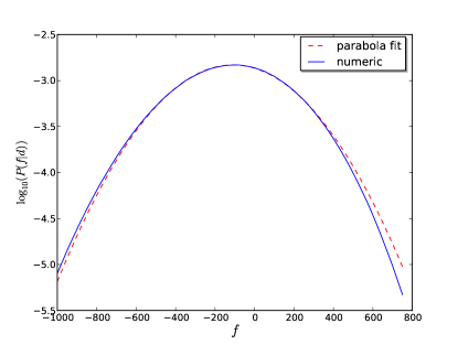
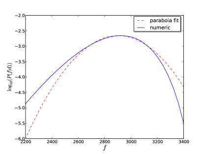
(a)                                                                         (b)

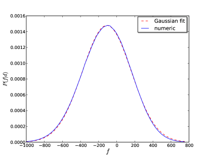
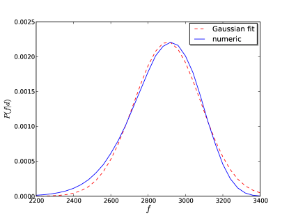
(c)                                                                         (d)

Figure 1: (color online) Normalized posterior distributions for $f$ in a one-dimensional test case with data generated from $f_{\text{gen}}=3$ [panels (a), and (c)] and $f_{\text{gen}}=3000$ [panels (b), and (d)]. The (a), (b) upper [(c), (d) lower] panels show the numerically calculated posterior including a parabola (Gaussian) fit. For $f_{\text{gen}}=3000$, the PDF is negatively skewed and thus significantly non-Gaussian. The fitting curves in the upper panels arise from translating the Gaussian fit of the lower panels into a quadratic function.

Note that there are no constraints regarding the response, except of its linearity in the primordial gravitational potential, and that the formalism itself is equally valid for correlated noise and for nonconstant priors on $f_{\text{nl}}$. The nonlinear corrections to the response $R$ arising from the nonlinear evolution of primordial perturbations have been shown to be small, $|f_{\text{nl}}|\sim\mathcal{O}(1)$, except for the lensing contributions of the late-time integrated Sachs-Wolfe effect (ISW). However, these nonlinear contributions can be absorbed in the $f_{\text{nl}}$ parameter with the result that the measurement of $f_{\text{nl}}$ is nonzero even if the initial $f_{\text{nl}}$ is zero Goldberg and Spergel (1999); Planck Collaboration et al. (2013b). We focus on uncorrelated noise and on a constant $f_{\text{nl}}$ prior for simplicity.

Moreover, we are able to calculate the maximum a posteriori estimator for $f_{\text{nl}}$, $f_{\text{MAP}}$ analytically by setting $\partial P(f|d)/\partial f\big{|}_{f=f_{\text{MAP}}}=0$. This yields

$$\begin{split}0=&\frac{1}{2}\text{tr}\bigg{\{}\frac{\partial}{\partial f}\ln\left(\frac{1}{2\pi}D^{-1}_{d,f}\right)\bigg{\}}\\ &+\frac{\partial H(d,m|f)}{\partial m}\frac{\partial m}{\partial f}+\frac{\partial H(d,m|f)}{\partial f}\bigg{|}_{f=f_{\text{MAP}}}.\end{split}$$ (21)

The exact solution after performing the partial derivatives can be found in Appendix B [Eqs. (40), (41)]. Note that we have used the implicit function theorem to calculate the partial derivative of the implicitly defined function $m(f)$ with respect to $f$. Here, too, we do not need any expensive sampling technique to determine $f_{\text{MAP}}$.

III Posterior validation and results

III.1 Validation approach

Now we introduce and apply the DIP test. This is an appropriate validation method for the $f_{\text{nl}}$ posterior, which not only is able to detect a mistake in the numerical implementation or the mathematical derivation of the posterior, but also reveals the kind of an error Dorn et al. (2013). For this, we use the following procedure Dorn et al. (2013); Cook et al. (2006):

1. Sample uniformly a value of $f_{\text{gen}}$ from an interval $I=\left[-f_{0},f_{0}\right]$, i.e., from a prior
   

   $$P(f)=\left\{\begin{array}[]{cc}\frac{1}{2f_{0}}&~{}~{}~{}~{}~{}~{}~{}~{}\text{if}~{}|f|<f_{0}\\ 0&\text{else}\end{array}\right..$$ (22)

2. Generate data $d$ for $f_{\text{gen}}$ according to Eq. (7).

3. Calculate a posterior curve for given data by determining $P(f|d)$ for $f\in I$ according to Eq. (20).

4. Calculate the posterior probability for $f\leq f_{\text{gen}}$ according to

   $$x:=\int_{-f_{0}}^{f_{\text{gen}}}\text{d}f~{}P(f|d)~{}\in\left[0,1\right].$$ (23)

5. If the calculation of the posterior was correct, the distribution for $x$, $P(x)$, should be uniform between 0 and 1.

We then check the uniformity of $P(x)$ numerically by going through steps 1–4 repeatedly.

III.2 Power spectrum

The second step of our validation scheme includes the drawing of a Gaussian random field $\phi$ from its covariance matrix $\Phi$. Considering the cosmic microwave background, we assume statistical homogeneity and isotropy for $\phi$, which leads to a diagonal covariance matrix $\Phi$ in the basis of spherical harmonics:

$$\Phi_{(lm)(l^{\prime}m^{\prime})}=\delta_{ll^{\prime}}\delta_{mm^{\prime}}C_{l},$$ (24)

where $l=0,1,\dots,l_{\max}$, $m=-l_{\max},\dots,l_{\max}$, and $C_{l}$ is the angular power spectrum of the CMB temperature anisotropies. The value $l_{\max}$ is determined by the discretization of the sphere. $C_{l}$ is generated with CAMB using the cosmological parameters from Ref. Bennett et al. (2013). In the following, we will consider data on $\mathcal{S}^{2}$ as well as one- and two-dimensional flat-sky toy cases.

When considering test cases of a flat data space in one and two dimensions, the covariance matrix of the primordial gravitational potential $\Phi$ is assumed to be diagonal in the corresponding Fourier space. We set $|k|=l$, where $k$ is a Fourier mode. Hence, $\Phi$ is given by

$$\Phi_{kk^{\prime}}=\delta_{kk^{\prime}}C_{k},$$ (25)

where $\delta_{kk^{\prime}}$ is the Kronecker delta symbol and we use the same power spectrum as on the sphere.

III.3 Flat position space

First, we consider one- and two-dimensional tests, for which the primordial gravitational potential is defined over an interval/area on a flat position space, which is discretized into 1024 pixels or, in the case of two dimensions, into 64$\times$64 pixels. For the response and noise covariance matrix, we assume the large-scale approximation with $\sigma^{2}_{n}=1.23\times 10^{-14}$, given in Eq. (10). The Gaussian random fields $\phi$ and $n$ were drawn from their covariance matrices $\Phi$ and $N$, respectively. Due to the fact that $M$ is diagonal, we can use Eq. (15) in our numerical implementations. Traces in Eq. (20) are determined by Operator Probing of the NIFTY package Selig et al. (2013) used for calculations throughout this paper.

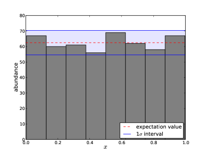
(a)

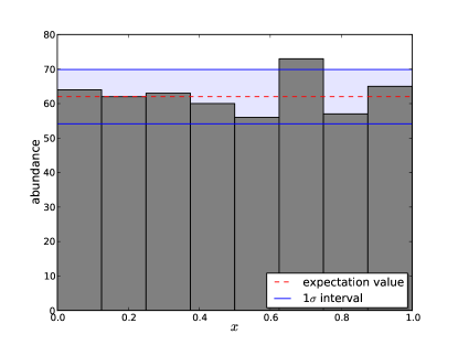
(b)

Figure 2: (color online) DIP distribution of calculated $x$ values for one- (a) and two-dimensional (b) test cases. The histograms show the un-normalized distribution of 500 $x$ values within eight bins. The standard deviation interval ($1\sigma$) around the expectation value as calculated from Poissonian statistics is also shown.

Figure 2 visualizes the numerical results in the one-dimensional and two-dimensional cases. The respective histograms show the un-normalized DIP distribution of 500 $x$ values calculated according to Eq. (23). A faulty posterior for $f_{\text{nl}}$ would emphasize abundances near to $x=0$ and $x=1$ Dorn et al. (2013); Cook et al. (2006), which is not the case. Therefore, these uniformly shaped distributions verify the accuracy of our posterior and justify the saddle-point approximation that we have made.

III.4 One-dimensional position space with Gaussian convolution

In the next test, we leave all specifications made in Sec. C in place but apply a Gaussian convolution with a constant standard deviation of $\sigma=1.3~{}\times$ (distance between the pixels) on the field $\phi$ when generating the data as a part of the response operation. Furthermore, we discretize the space into 256 pixels for simplicity. The convolution causes a nondiagonal response matrix and thus a nondiagonal $M$. Therefore, we have to use the general Eqs. (13), (14) in our numerical implementation.

Figure 3 shows the numerical result. The histogram, showing the un-normalized DIP distribution of 500 $x$ values within eight bins, does not emphasize abundances near to $x=0$ and $x=1$. Thus, the uniformly shaped distribution again verifies the accuracy of the posterior and justifies our saddle-point approximation.

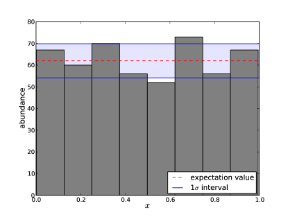
Figure 3: (color online) DIP distribution of calculated $x$ values for the one-dimensional test case with Gaussian convolution. The histogram shows the un-normalized distribution of 500 $x$ values within eight bins. The standard deviation interval ($1\sigma$) around the expectation value as calculated from Poissonian statistics is also shown.

III.5 Data on the sphere

Finally, we consider the primordial gravitational potential on the sphere $\mathcal{S}^{2}$. For the implementation, we use the HEALPix package to discretize the sphere into $12N^{2}_{\text{side}}$ pixels. We still use the large-scale approximation with $\sigma^{2}_{n}=1.23\times 10^{-14}$ and $N_{\text{side}}=32$.

Figure 4 visualizes the numerical result. The histogram shows again the un-normalized DIP distribution of 500 $x$ values within eight bins. In marked contrast to the flat space test cases, abundances near to $x=0$ and $x=1$ are highly emphasized, which indicates an insufficient posterior. The convex “$\cup$ shape” of the distribution indicates an underestimation ($\approx 35\%$) of the standard deviation $\sigma_{f}$ of our numerical implementation of the posterior with respect to the correct $f_{\text{nl}}$ posterior (see DIP test, Ref. Dorn et al. (2013), for details). Due to the fact that we changed only the basis of the space in comparison to the Cartesian tests (see Secs. III C, III D), the test failure, and thus the underestimation of the standard deviation, is likely due to the insufficient precision of the numerical transformations between the basis of spherical harmonics and the HEALPix space and thus numerical in nature. In particular, in the used implementation, these transformations are applied repeatedly, whereby the respective errors of the single transformations accumulate to a significant inaccuracy. We want to emphasize that other $f_{\text{nl}}$ estimators might be affected by this problem as well (depending on their particular implementation).

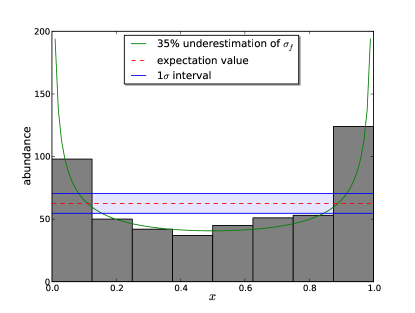
Figure 4: (color online) DIP distribution of calculated $x$ values for the test case on the sphere. The histogram shows the un-normalized distribution of 500 $x$ values within eight bins. The standard deviation interval ($1\sigma$) around the expectation value as calculated from Poissonian statistics is also shown. The green curve shows the analytical shape of a Gaussian posterior distribution whose standard deviation deviates by $35\%$ from the one of the true Gaussian posterior.

III.6 Reconstruction of the primordial gravitational potential

Up to now, we have focused on the accuracy of the $f_{\text{nl}}$ posterior. However, we are also able to reconstruct the primordial gravitational potential $\varphi$ or the auxiliary Gaussian field $\phi$ from the data $d$. For this, we assume the minimum of the Hamiltonian up to quadratic order in $f$ [see Eqs. (8), (9), (13)] to be a precise estimate for $\phi$. $\varphi$ is reconstructed by applying a Wiener Filter Wiener (1949) on the data, given by

$$m_{w}=\left(\Phi^{-1}+R^{\dagger}N^{-1}R\right)^{-1}R^{\dagger}N^{-1}d=Dj.$$ (26)

Figure 5 shows an example of this reconstruction, where we have used the specifications made in Sec. E with $N_{\text{side}}=32$, $f_{\text{nl}}=2000$, and $\sigma_{n}^{2}=0.5\times 10^{-11}$. We have chosen this large value of $f_{\text{nl}}$ and $\sigma_{n}^{2}$ to demonstrate the reconstruction at a high level of non-Gaussianity and noise.

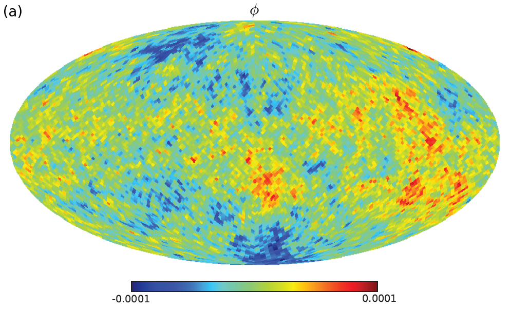
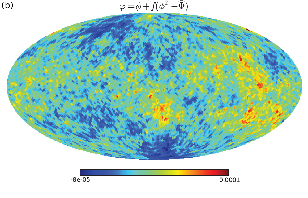
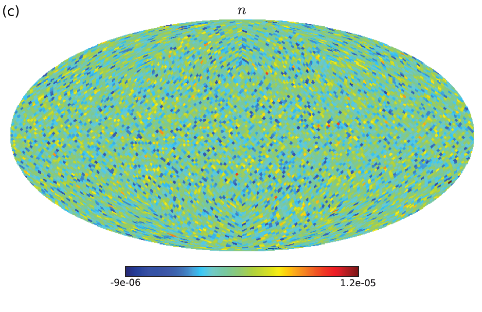
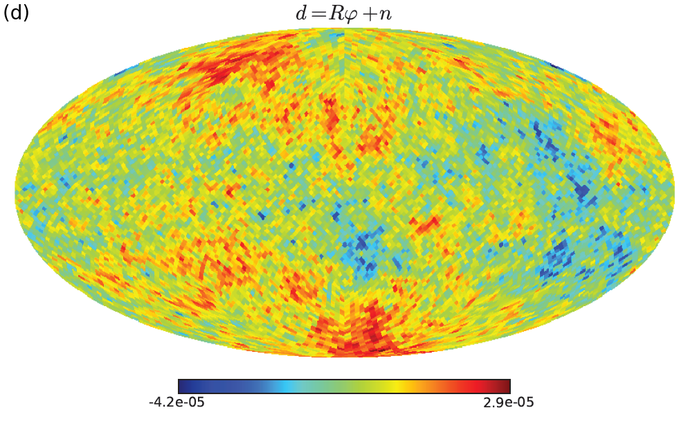
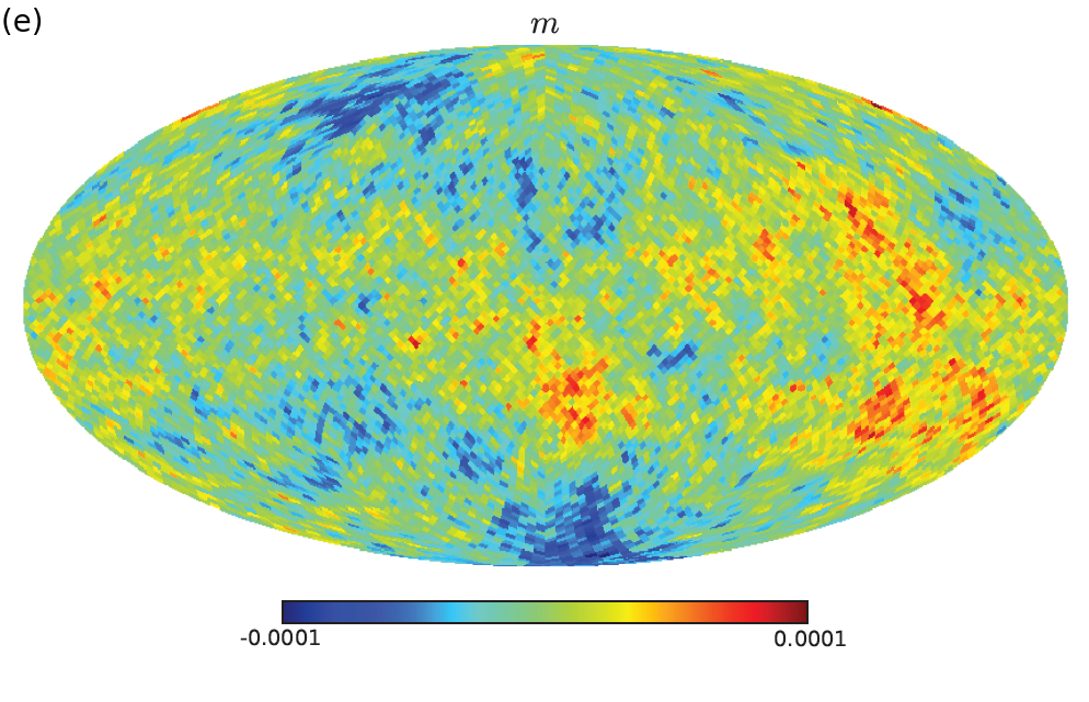
Figure 5: (color online) Reconstruction of the primordial gravitational potential $\varphi$ or the auxiliary Gaussian field $\phi$ by using the maximum of the Hamiltonian and by applying a Wiener Filter, respectively. The upper four panels [(a)–(d)] are showing the generation of the mock data $d$, whereas the last two panels [(e), (f)] are showing the reconstructions of the original fields. Note the different color codes.

III.7 Comparison to the KSW estimator for $f_{\text{nl}}$

A common procedure to determine the level of non-Gaussianity is the application of the KSW estimator developed in Komatsu et al. (2005) for $f_{\text{nl}}$, which uses the CMB-bispectrum and is given by Komatsu et al. (2005); Enßlin et al. (2009)

$$\hat{f}_{KSW}=\frac{1}{\mathcal{N}}m_{w}^{\dagger}\Phi^{-1}m_{w}^{2}$$ (27)

with the data-independent normalization constant

$$\mathcal{N}=\left\langle m_{w}^{\dagger}\Phi^{-1}m_{w}^{2}\right\rangle_{(d,s|f=1)}$$ (28)

and the standard deviation $\sigma_{\hat{f}_{\text{{KSW}}}}=1/\sqrt{\mathcal{N}}$. This means the PDF for $f_{\text{nl}}$ is Gaussian, given by $\mathcal{G}(\hat{f}_{\text{{KSW}}},\sigma_{\hat{f}_{\text{{KSW}}}}^{2})$. Note that the standard deviation $\sigma_{\hat{f}_{\text{{KSW}}}}$ can also be obtained by sampling the PDF of the KSW-estimator and reading off its value.

The first difference in comparison to our posterior is the reduction of a PDF to a single number, and as a consequence thereof, a large loss of information. In particular, this becomes problematic if the PDF is not symmetric around the estimated value. The second difference is the data independence of the uncertainty, determined by averaging over data and signal realizations, given a unit $f_{\text{nl}}$.

To visualize the influence of these effects on the accuracy of the KSW estimator, we apply the DIP test to the latter with the numerical settings made in III C for the one-dimensional case, but use $\sigma_{n}^{2}=10^{-15}$, and a white power spectrum in position space, $\sigma_{\phi}^{2}=10^{-10}$. We perform the DIP test within the intervals $I_{1}=[-6000,6000]$ and $I_{2}=[-2000,2000]$. The normalization $\mathcal{N}$ is calculated from $1.06\times 10^{8}$ data realizations. The results are shown in Fig. 6.

The characteristic and significant “$\cup$” shape of the (a) upper-left and (b) upper-right DIP distribution in Fig. 6 encodes an underestimation of the standard deviation $\sigma_{\hat{f}_{\text{{KSW}}}}$ on average (for details, see Ref. Dorn et al. (2013)), whereas for our posterior we obtain a flat distribution [see (c) the lower DIP distribution]. The underestimation arises from the wrong assumption of symmetric errors with respect to $\hat{f}_{\text{{KSW}}}$ for large values of the underlying, true value of $f_{\text{nl}}$. However, with a decreasing value of $f_{\text{nl}}$, the distribution becomes flatter and will be uniform in the limit of small values of $f_{\text{nl}}$.

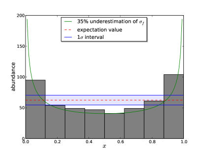
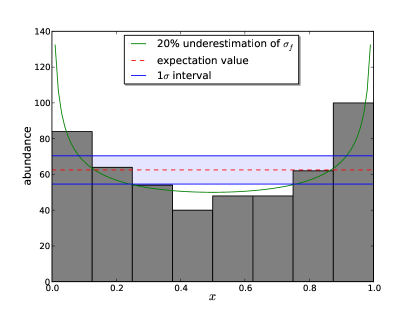
(a)                                                                             (b)

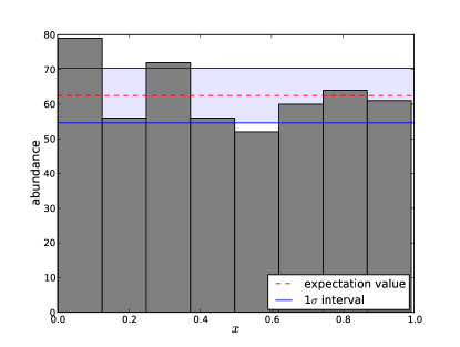
(c)

Figure 6: (color online) DIP distributions of calculated $x$ values for the KSW estimator [(a) upper left, (b) upper right] and approximated posterior according to Eq. (20) [(c) lower] and according to the intervals $I_{1}=[-6000,6000]\ni f_{\text{nl}}$ (left, right), $I_{2}=[-2000,2000]\ni f_{\text{nl}}$ (middle). The histograms show the un-normalized distributions of 500 $x$ values within eight bins. The standard deviation interval ($1\sigma$) around the expectation value as calculated from Poissonian statistics is also shown. The (green) fit in the (a) upper-left [(b) upper-right] panel is a theoretical DIP distribution calculated with a Gaussian posterior, whose standard deviation was underestimated by 35% (20%).

Another difference between the estimator and our posterior is the computational cost. In particular, the KSW estimator needs an average over different data realizations in addition to that over signal realizations. Our approach, however, requires only the latter, and we can perform it largely analytically.

III.8 Differences from previous Bayesian methods

To call attention to differences from previous Bayesian methods we briefly compare our posterior to methods pointed out in (a) Ref. Elsner et al. (2010) and (b) Ref. Verde et al. (2013).

(a) To infer the value of $f_{\text{nl}}$ in this work, closed-form expressions for the joint $f_{\text{nl}}$ posterior are presented. Then, Hamiltonian sampling algorithms are used to finally obtain the posterior of $f_{\text{nl}}$. In comparison to this method, we do not need such an expensive sampling method to infer the value of $f_{\text{nl}}$, because we got rid of the $\phi$ marginalization by replacing the exact Hamiltonian by its Taylor expansion and performing the $\phi$ integration afterwards analytically (see Sec. II B).

(b) Here, the authors derive an exact expression for the $f_{\text{nl}}$ posterior. However, this formula cannot be performed analytically. To circumvent this problem, a second-order Edgeworth expansion (in $f_{\text{nl}}$), i.e. a Taylor expansion of the full exponential $e^{-H}$, is used, which works for small values of $f_{\text{nl}}$. In marked contrast to this approximation, we Taylor-expand the Hamiltonian $H$ in the small field $\phi$ ($\propto\mathcal{O}(10^{-5})$) up to second order and not in $f_{\text{nl}}$. By this, we guarantee that the Taylor expansion is well justified even for high values of $f_{\text{nl}}$. Apart from this, Edgeworth expansions can be problematic, because the positivity of the approximative PDF cannot be guaranteed in general.

III.9 Shape of the $f_{\text{nl}}$ posterior

In order to investigate the shape of the $f_{\text{nl}}$ posterior we consider the one-dimensional test case presented in Sec. III C. In agreement with results concerning $f_{\text{nl}}$-estimators, e.g. Ref. Smith et al. (2011), our posterior can deviate from a Gaussian. While for $f_{\text{nl}}\approx 0$ the PDF is approximately Gaussian, for $f_{\text{nl}}\gg 0$ it is negatively skewed, and for $f_{\text{nl}}\ll 0$ it is positively skewed. The deviations for $f_{\text{nl}}\neq 0$ arise mainly from the determinant part of Eq. (20) and increase with the value of $f_{\text{nl}}$. Figure 1 illustrates this effect. The small deviations for $f_{\text{nl}}=3$ do not emerge due to a nonvanishing $f_{\text{nl}}$, but arise during the generation of the Gaussian random field $\phi$, which contains tiny correlations between small and large scales. However, the PDF for $f_{\text{nl}}=3$ is Gaussian on average. Although the deviations from a Gaussian can be neglected in practice for realistic values of $f_{\text{nl}}$, constrained recently by the Planck Collaboration to be $f_{\text{nl}}=2.7\pm 5.8$ ($68\%$ C.L. statistical) Planck Collaboration et al. (2013b), we want to stress that the general approach of non-Gaussianity estimation and posterior verification can be applied to other forms of non-Gaussianity as well.

IV The Bayesian $g_{\text{nl}}$-posterior

Until now we have focused on first-order deviations from Gaussianity (i.e. deviations from Gaussianity are dominated by the bispectrum), which are characterized by the $f_{\text{nl}}$ parameter. Now we want to extend our formalism to higher-order deviations. The next-leading order is described by the trispectrum, which can be parametrized by the so-called $g_{\text{nl}}$ parameter. If we take $g_{\text{nl}}$ into account, the primordial gravitational potential reads Verde et al. (2013)

$$\tilde{\varphi}=\phi+f_{\text{nl}}\left(\phi^{2}-\widehat{{\Phi}}\right)+g_{\text{nl}}\left(\phi^{3}-3\phi\star\widehat{{\Phi}}\right).$$ (29)

One has to consider this order, for instance, if deviations from Gaussianity are significantly influenced by the trispectrum or even dominated by it. Here we consider the latter, i.e. $f_{\text{nl}}\approx 0$, to avoid too lengthy formulas. Thus, the data are given by

$$d=R\left(\phi+g_{\text{nl}}\left(\phi^{3}-3\phi\star\widehat{{\Phi}}\right)\right)+n,$$ (30)

and the information Hamiltonian by

$$\begin{split}H(d,\phi|g)=&H_{0}+\frac{1}{2}\phi^{\dagger}D^{-1}\phi-j^{\dagger}\phi\\ &+\sum_{n=0}^{6}\frac{1}{n!}\Omega^{(n)}[\phi,\dots,\phi],\end{split}$$ (31)

with the additional (in comparison to Sec. II) abbreviations

$$\begin{split}g=&~{}g_{\text{nl}},~{}\Omega^{(0)}=0=\Omega^{(5)}_{xyzuv}\\ \Omega^{(1)}_{x}=&~{}3g_{x}\hat{\Phi}_{x}j_{x},\\ \Omega^{(2)}_{xy}=&~{}\big{(}\frac{9}{2}g_{x}\hat{\Phi}_{x}M_{xy}g_{y}\hat{\Phi}_{y}-3M_{xy}g_{y}\hat{\Phi}_{y}\\ &+1~{}\text{perturbation}\big{)},\\ \Omega^{(3)}_{xyz}=&~{}\big{(}-\left(gj\right)_{x}\delta_{xy}\delta_{xz}+5~{}\text{perturbations}\big{)},\\ \Omega^{(4)}_{xyzu}=&~{}(M_{xy}g_{y}\delta_{yz}\delta_{yu}-3g_{x}M_{xy}g_{y}\hat{\Phi}_{y}\delta_{yz}\delta_{yu}\\ &+23~{}\text{perturbations}),\\ \Omega^{(6)}_{xyzuvw}=&~{}(\frac{1}{2}\delta_{xy}\delta_{zy}g_{y}M_{yu}g_{u}\delta_{uv}\delta_{uw}\\ &+719~{}\text{perturbations}).\end{split}$$ (32)

Now we are able to perform again a saddle-point approximation in the primordial gravitational potential around the minimum of $H(d,\phi|g)$. The minimum $\tilde{m}$ and the Hessian $D^{-1}_{d,g}$ of the Hamiltonian are given by

$$\begin{split}0=&\left(D^{-1}+\Omega^{(2)}\right)\tilde{m}-j+\left(\Omega^{(1)}\right)^{\dagger}\\ &-3gj\star\tilde{m}^{2}+3g\bigg{(}\frac{1}{3}M\tilde{m}^{3}+\tilde{m}^{2}\star M\tilde{m}-gM\left(\hat{\Phi}\star\tilde{m}^{3}\right)\\ &-3g\left(\hat{\Phi}\star\tilde{m}^{2}\right)\star M\tilde{m}\bigg{)}+3g^{2}\tilde{m}^{2}\star M\tilde{m}^{3}\end{split}$$ (33)

and

$$\begin{split}&\left(D^{-1}_{d,g}\right)_{xy}=D^{-1}_{xy}+\Omega^{(2)}_{xy}-6g~{}j_{x}\tilde{m}_{x}\delta_{xy}+6g\bigg{(}M_{xy}\tilde{m}^{2}_{y}\\ &+\tilde{m}_{x}(M\tilde{m})_{x}\delta_{xy}-3g\big{(}M_{xy}\hat{\Phi}_{y}\tilde{m}^{2}_{y}+\hat{\Phi}_{x}\tilde{m}_{x}(M\tilde{m})_{x}\delta_{xy}\big{)}\bigg{)}\\ &+6g^{2}\left(\tilde{m}_{x}\left(M\tilde{m}^{3}\right)_{x}\delta_{xy}+\frac{3}{2}\tilde{m}^{2}_{x}M_{xy}\tilde{m}^{2}_{y}\right),\end{split}$$ (34)

if we assume $g_{\text{nl}}$ to be a scalar. Thus, the posterior for $g_{\text{nl}}$ can be calculated as follows:

$$\begin{split}&\ln(P(g|d))=-H(g|d)\\ &=-\frac{1}{2}\text{tr}\left[\ln\left(\frac{1}{2\pi}D_{d,g,\text{diag}}^{-1}\right)\right]\\ &~{}~{}~{}~{}+\frac{1}{2}\text{tr}\left[\sum_{n=1}^{\infty}\frac{(-1)^{n}}{n}\left(D_{d,g,\text{diag}}D_{d,g,\text{non-diag}}^{-1}\right)^{n}\right]\\ &~{}~{}~{}~{}-H(d,\tilde{m}|g)+\text{const.}\end{split}$$ (35)

Analogous to Eq. (20) the series expansion can be truncated if the terms become sufficiently small.

Note that our formalism does not require a value of $f_{\text{nl}}\approx 0$. One can easily include $f_{\text{nl}},~{}g_{\text{nl}}$ and even higher-order corrections into the Hamiltonian and is still able to do the stated Taylor expansion due to the fact that the expansion parameter is $\phi$ and not $f_{\text{nl}}$ or $g_{\text{nl}}$.

V Concluding remarks

We derived a precise probability density function for the non-Gaussianity parameter $f_{\text{nl}}$ in the framework of information field theory. For this, we considered temperature anisotropies of the cosmic microwave background. During this calculation, we used a saddle-point approximation by performing a Taylor expansion around the minimum of the so-called information Hamiltonian [see Eqs. (13), (14)] and assumed a linear response of the data to the primordial gravitational potential $\varphi$, Gaussian noise, and an $f_{\text{nl}}$-independent prior, $P(f)$. The precision of the posterior was validated by the DIP test (see Sec. III A and Refs. Dorn et al. (2013); Cook et al. (2006)).

In the application examples concerning a flat sky (see Secs. III C and III D), we have verified the precision of the derived posterior, whereas in the test case on the sphere (see Sec. III.E), we have shown its numerical insufficiency. One likely reason for this failure is the insufficient precision of the numerical transformations between the basis of spherical harmonics and the HEALPix space, since the basis transformations are the only qualitative difference between the failed spherical test and the successful Cartesian tests. As a consequence of this, it would be necessary to investigate the numerical precision of the basis transformations on the sphere Reinecke (2011); Reinecke and Sverre Seljebotn (2013) in order to ensure that published $f_{\text{nl}}$ estimators Planck Collaboration et al. (2013b) are not affected by this.

A comparison to the KSW estimator (see Sec. III G) revealed a precise performance of the derived $f_{\text{nl}}$ posterior even for high values of $f_{\text{nl}}$, while the uncertainty estimate for the KSW estimator is becoming worse with an increasing (high) value of $f_{\text{nl}}$.

Furthermore, we have presented a well-working nonlinear reconstruction method for the primordial gravitational field $\varphi$ on the sphere $\mathcal{S}^{2}$ (see Sec. III F) and have investigated the shape of the $f_{\text{nl}}$ posterior (see Sec. III I), which is negatively (positively) skewed for $f_{\text{nl}}\gg 0~{}(f_{\text{nl}}\ll 0)$ and Gaussian for $f_{\text{nl}}\approx 0$ (e.g. Ref. Smith et al. (2011)).

Note that by including a Gaussian convolution in the response on the primordial gravitational field, we have shown that more complex cases than the Sachs-Wolfe limit of local response can be dealt with. Therefore, the presented method should also be applicable to Planck CMB maps at full resolution when efficient and accurate transformations (for instance, between the three-dimensional position space) are used Elsner and Wandelt (2010).

Finally, we have extended our formalism to the next leading order of non-Gaussianity, which can be parametrized by $g_{\text{nl}}$, in Sec. IV, and have explained how to even go beyond this.

Appendix A Functional derivatives of the Hamiltonian

Equations (13) and (14) are based on

$$\begin{split}&\frac{\delta}{\delta\phi(w)}{\Lambda^{(3)}}[\phi,\phi,\phi]\\ &=6f\frac{\delta}{\delta\phi(w)}\int\text{d}x\int\text{d}y\int\text{d}z~{}\phi(y)M(y,x)~{}~{}~{}~{}~{}~{}~{}~{}~{}~{}~{}~{}~{}~{}~{}~{}~{}~{}~{}~{}~{}~{}~{}~{}~{}~{}~{}~{}~{}\\ &~{}~{}~{}\times\delta(x-z)\phi(x)\phi(z)\\ &=6f\frac{\delta}{\delta\phi(w)}\int\text{d}x\int\text{d}y~{}\phi(y)M(y,x)\phi^{2}(x)\\ &=6f\int\text{d}x\int\text{d}y~{}\delta(y-w)M(y,x)\phi^{2}(x)\\ &~{}~{}~{}+12f\int\text{d}x\int\text{d}y~{}\phi(y)M(y,x)\phi(x)\delta(w-x)\\ &=(6fM\phi^{2}+12f\phi\star M\phi)(w)\end{split}$$ (36)

$$\begin{split}&\frac{\delta^{2}}{\delta\phi(w)\delta\phi(v)}{\Lambda^{(3)}}[\phi,\phi,\phi]\\ &=6(2f\int\text{d}x~{}M(w,x)\phi(x)\delta(x-v)\\ &~{}~{}~{}+2f\int\text{d}y~{}\phi(w)M(w,y)\delta(y-v)~{}~{}~{}~{}~{}~{}~{}~{}~{}~{}~{}~{}~{}~{}~{}~{}~{}~{}~{}~{}~{}~{}~{}~{}~{}~{}~{}~{}~{}~{}~{}~{}~{}~{}~{}~{}~{}~{}~{}~{}~{}~{}~{}~{}~{}~{}~{}~{}~{}~{}~{}~{}~{}~{}~{}~{}~{}~{}~{}~{}~{}~{}~{}~{}~{}~{}~{}~{}\\ &~{}~{}~{}+2f\int\text{d}y~{}\phi(y)M(y,w)\delta(w-v))\\ &=(6(4f\phi\star M+2f\widehat{M\phi}))(w,v)\end{split}$$ (37)

$$\begin{split}&\frac{\delta}{\delta\phi(w)}\Lambda^{(4)}[\phi,\phi,\phi,\phi]\\ &=24(\frac{f^{2}}{2}\frac{\delta}{\delta\phi(w)}\int\text{d}x\int\text{d}v~{}\phi^{2}(x)M(x,v)\phi^{2}(v))~{}~{}~{}~{}~{}~{}~{}~{}~{}~{}~{}~{}~{}~{}~{}~{}~{}~{}~{}~{}~{}~{}~{}~{}~{}~{}~{}~{}~{}~{}~{}~{}~{}~{}~{}~{}~{}~{}~{}~{}~{}~{}~{}~{}~{}~{}~{}~{}~{}~{}~{}~{}~{}~{}~{}~{}~{}~{}~{}\\ &=24(f^{2}\int\text{d}v~{}\phi(w)M(w,v)\phi(v)^{2}\\ &~{}~{}~{}+f^{2}\int\text{d}x~{}\phi(x)^{2}M(x,w)\phi(w))\\ &=(48f^{2}\phi\star M\phi^{2})(w)\end{split}$$ (38)

$$\begin{split}&\frac{\delta^{2}}{\delta\phi(w)\delta\phi(v)}\Lambda^{(4)}[\phi,\phi,\phi,\phi]\\ &=24(4f^{2}\int\text{d}x~{}\phi(w)M(w,x)\phi(x)\delta(x-v)\\ &~{}~{}~{}+2f^{2}\int\text{d}x~{}\delta(w-v)M(w,x)\phi^{2}(x))~{}~{}~{}~{}~{}~{}~{}~{}~{}~{}~{}~{}~{}~{}~{}~{}~{}~{}~{}~{}~{}~{}~{}~{}~{}~{}~{}~{}~{}\\ &=(24(4f^{2}\phi^{2}\star M+2f^{2}\widehat{M\phi^{2}}))(w,v)\end{split}$$ (39)

Appendix B Analytic solution of the MAP-estimator for $f_{\text{nl}}$

Performing the partial derivatives of Eq. (21) yields

$$\begin{split}&\frac{1}{2}\text{tr}\bigg{\{}D_{d,f}\big{(}\Lambda^{(2)}_{f}+fm\star M+2\widehat{Mm}+8fm^{2}\star M\\ &+4f\widehat{Mm^{2}}\big{)}\bigg{\}}-\bigg{\{}\left(D^{-1}+\Lambda^{(2)}\right)m-j+\Lambda^{(1)}\\ &+fMm^{2}+2fm\star Mm+2f^{2}m\star Mm^{2}\bigg{\}}^{\dagger}D_{d,f}\\ &\times\bigg{\{}Mm^{2}+2m\star Mm+4fm\star Mm^{2}\bigg{\}}\\ &+\sum_{n=0}^{4}\frac{1}{n!}\Lambda^{(n)}_{f}[\phi,\cdots,\phi]=0,\end{split}$$ (40)

with the abbreviations

$$\begin{split}\Lambda^{(0)}_{f}&=j^{\dagger}\widehat{\Phi}+f\widehat{\Phi}^{\dagger}M\widehat{\Phi},\\ \Lambda^{(1)}_{f}&=-\widehat{\Phi}^{\dagger}M,\\ \Lambda^{(2)}_{f}&=-2\widehat{j^{\prime}},\\ \left(\Lambda^{(3)}_{f}\right)_{xyz}&=(M_{xy}\delta_{yz}+\text{5 perturbations}),\\ \left(\Lambda^{(4)}_{f}\right)_{xyzu}&=(f_{x}\delta_{xy}M_{yz}\delta_{zu}+\text{23 perturbations}).\end{split}$$ (41)

References

- Bennett et al. (2013) C. L. Bennett, D. Larson, J. L. Weiland, N. Jarosik, G. Hinshaw, N. Odegard, K. M. Smith, R. S. Hill, B. Gold, M. Halpern, et al., Astrophys. J. Suppl. Ser. 208, 20 (2013), eprint 1212.5225.
- Planck Collaboration et al. (2013a) Planck Collaboration, P. A. R. Ade, N. Aghanim, C. Armitage-Caplan, M. Arnaud, M. Ashdown, F. Atrio-Barandela, J. Aumont, C. Baccigalupi, A. J. Banday, et al., ArXiv e-prints (2013a), eprint 1303.5076.
- Planck Collaboration et al. (2013b) Planck Collaboration, P. A. R. Ade, N. Aghanim, C. Armitage-Caplan, M. Arnaud, M. Ashdown, F. Atrio-Barandela, J. Aumont, C. Baccigalupi, A. J. Banday, et al., ArXiv e-prints (2013b), eprint 1303.5084.
- Bartolo et al. (2004) N. Bartolo, E. Komatsu, S. Matarrese, and A. Riotto, Physical Reports 402, 103 (2004), eprint arXiv:astro-ph/0406398.
- Falk et al. (1993) T. Falk, R. Rangarajan, and M. Srednicki, ApJL 403, L1 (1993), eprint arXiv:astro-ph/9208001.
- Gangui (1994) A. Gangui, Phys. Rev. D 50, 3684 (1994), eprint arXiv:astro-ph/9406014.
- Salopek and Bond (1990) D. S. Salopek and J. R. Bond, Phys. Rev. D 42, 3936 (1990).
- Peebles (1999) P. J. E. Peebles, Astrophys. J. 510, 523 (1999), eprint arXiv:astro-ph/9805194.
- Komatsu and Spergel (2001) E. Komatsu and D. N. Spergel, Phys. Rev. D 63, 063002 (2001), eprint arXiv:astro-ph/0005036.
- Bardeen et al. (1983) J. M. Bardeen, P. J. Steinhardt, and M. S. Turner, Phys. Rev. D 28, 679 (1983).
- Komatsu (2002) E. Komatsu, ArXiv Astrophysics e-prints (2002), eprint arXiv:astro-ph/0206039.
- Komatsu et al. (2005) E. Komatsu, D. N. Spergel, and B. D. Wandelt, Astrophys. J. 634, 14 (2005), eprint arXiv:astro-ph/0305189.
- Creminelli et al. (2007) P. Creminelli, L. Senatore, and M. Zaldarriaga, Journal of Cosmology and Astro-Particle Physics 3, 019 (2007), eprint arXiv:astro-ph/0606001.
- Smith et al. (2011) T. L. Smith, M. Kamionkowski, and B. D. Wandelt, Phys. Rev. D 84, 063013 (2011), eprint 1104.0930.
- Elsner and Wandelt (2010) F. Elsner and B. D. Wandelt, Astrophys. J. 724, 1262 (2010), eprint 1010.1254.
- Elsner et al. (2010) F. Elsner, B. D. Wandelt, and M. D. Schneider, Astronomy and Astrophysics 513, A59 (2010), eprint 1002.1713.
- Enßlin et al. (2009) T. A. Enßlin, M. Frommert, and F. S. Kitaura, Phys. Rev. D 80, 105005 (2009), eprint 0806.3474.
- Verde et al. (2013) L. Verde, R. Jimenez, L. Alvarez-Gaume, A. F. Heavens, and S. Matarrese, Journal of Cosmology and Astro-Particle Physics 6, 023 (2013), eprint 1301.6017.
- Dorn et al. (2013) S. Dorn, N. Oppermann, and T. A. Enßlin, Phys. Rev. E 88, 053303 (2013).
- Sachs and Wolfe (1967) R. K. Sachs and A. M. Wolfe, Astrophys. J. 147, 73 (1967).
- White and Hu (1997) M. White and W. Hu, Astronomy and Astrophysics 321, 8 (1997), eprint arXiv:astro-ph/9609105.
- Bayes (1763) T. Bayes, Phil. Trans. of the Roy. Soc. 53, 370 (1763).
- Seljak and Zaldarriaga (1996) U. Seljak and M. Zaldarriaga, Astrophys. J. 469, 437 (1996), eprint arXiv:astro-ph/9603033.
- Lewis et al. (2000) A. Lewis, A. Challinor, and A. Lasenby, Astrophys. J. 538, 473 (2000), eprint arXiv:astro-ph/9911177.
- Doran (2005) M. Doran, Journal of Cosmology and Astro-Particle Physics 10, 011 (2005), eprint arXiv:astro-ph/0302138.
- Selig et al. (2013) M. Selig, M. R. Bell, H. Junklewitz, N. Oppermann, M. Reinecke, M. Greiner, C. Pachajoa, and T. A. Enßlin, Astronomy and Astrophysics 554, A26 (2013), eprint 1301.4499.
- Goldberg and Spergel (1999) D. M. Goldberg and D. N. Spergel, Phys. Rev. D 59, 103002 (1999), eprint arXiv:astro-ph/9811251.
- Cook et al. (2006) S. R. Cook, A. Gelman, and D. B. Rubin, Journal of Computational and Graphical Statistics 15, 675 (2006).
- Wiener (1949) N. Wiener, Extrapolation, Interpolation, and Smoothing of Stationary Time Series (New York: Wiley, 1949), ISBN 9780262730051.
- Reinecke (2011) M. Reinecke, Astronomy and Astrophysics 526, A108 (2011), eprint 1010.2084.
- Reinecke and Sverre Seljebotn (2013) M. Reinecke and D. Sverre Seljebotn, ArXiv e-prints (2013), eprint 1303.4945.
- Gòrski et al. (2005) K. M. Gòrski, E. Hivon, A. J. Banday, B. D. Wandelt, F. K. Hansen, M. Reinecke, and M. Bartelmann, The Astrophysical Journal 622, 759 (2005).