Fluid limits to analyze long-term flow rates of a stochastic network with ingress discarding

Abstract

We study a simple rate control scheme for a multiclass queuing network for which customers are partitioned into distinct flows that are queued separately at each station. The control scheme discards customers that arrive to the network ingress whenever any one of the flow’s queues throughout the network holds more than a specified threshold number of customers. We prove that if the state of a corresponding fluid model tends to a set where the flow rates are equal to target rates, then there exist sufficiently high thresholds that make the long-term average flow rates of the stochastic network arbitrarily close to these target rates. The same techniques could be used to study other control schemes. To illustrate the application of our results, we analyze a network resembling a 2-input, 2-output communications network switch.

T1Supported in part by NSF Grants ANI-0331659, CNS-0953884 and CNS-0910702.

and

1 Introduction

We consider a multiclass queuing network whose customers are partitioned into $F$ distinct flows. Customers of a flow $f\in\{1,\ldots,F\}$ arrive according to an independent renewal process and follow a fixed, acyclic sequence of stations. The service times at each station are also independent. Each flow $f$ has a weight $w_{f}\in\mathbb{R}_{+}$, and each of $d$ stations is equipped with per-flow queues and serves a flow in proportion to its weight using a weighted round robin or a similar queueing discipline like weighted fair queueing or generalized head of line processor sharing.

We consider a simple scheme which we call ingress discarding for admitting customers. The ingress discarding scheme works as follows. Whenever any of a flow’s queues exceed a threshold $h$, that flow’s customers are discarded at the network ingress. There are two main objectives of the scheme: (i) stability when the arrival rates in the absence of discarding would cause the utilization of some stations to exceed 1, and (ii) fairness in the long-term average departure rates when the network cannot accommodate all the incoming flows. The contribution of this article is a methodology for proving that the long-term average flow rates in such a network can be made arbitrarily close to those predicted by a fluid model, provided that the discarding thresholds are sufficiently high.

There are a number of applications of such a control policy. One application is for service centers such as call centers. It might be acceptable to block incoming customers, but unacceptable to drop customers that have been admitted to the system, hence the appropriateness of ingress discarding. A designer of such a system might want to show that the flow rates of various types of customers are fair in some sense. This work can be used to show that if the system’s fluid model achieves fair rates, then the system will achieve close to fair rates provided that the discarding thresholds are sufficiently high. Another application area is in data-packet switch design. A packet switch typically consists of several line-cards that transmit and receive the data packets, and a switch-fabric that serves as an interconnect. A design requirement might be that any packet discarding occur in the line-cards rather than in the switch fabric, since the line cards are better equipped to record statistics about the dropped packets, for instance. The switch fabric can be thought of as a queuing network, and ingress discarding would be one way to fulfill the requirement that discarding only occur in the line cards. Again, this work shows that the flow rates of such a system approach those predicted by a fluid model if the discarding thresholds are made sufficiently high.

To illustrate our methodology, we consider the simple network in Figure 1.

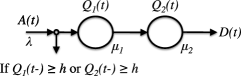
Figure 1: A queueing network with input discarding.

This network carries a single flow and customers arrive as a renewal process $E(t)$. There are two queues, each with i.i.d. service times with mean $\mu_{i}^{-1}$ in queue $i$ ($i=1,2$). Designate by $Q_{i}(t)$ the length of queue $i$ ($i=1,2$). The ingress discarding scheme discards the arrivals that occur when one of the two lengths is at least equal to threshold $h$. We want to show that if the thresholds are made large enough factor $n$, that the flow rates approach $\min\{\lambda,\mu_{1},\mu_{2}\}$. More precisely, we want to show that for every $\epsilon>0$ there exists some $n_{\epsilon}$ such that if threshold scale factor $n\geq n_{\epsilon}$, then the average rate of the departure process $D(t)$ exceeds $\min\{\lambda,\mu_{1},\mu_{2}\}-\epsilon$. Note that since we scale the thresholds by a factor $n$, the starting value of the threshold $h$ is not important, so long as it is positive. Also note that we do not attempt to derive any result on the speed of convergence—how fast $nh$ must grow to achieve rates within a smaller and smaller $\epsilon$ of the desired rates.

The analysis approach, which we believe can be extended to control strategies that change admission, service, or routing behavior when queue depths cross thresholds that can be made large, is based on deriving properties of the stochastic network using a fluid model. However for clarity of exposition, we limit our focus in this paper to the ingress discarding policy. As in work by Dai Dai95 we take a fluid limit by considering a sequence of larger and larger initial conditions, and scaling time and space by the size of those initial conditions. However, in order to consider stochastic networks with larger and larger thresholds, our fluid limit also considers a sequence of systems with thresholds scaled by an increasing factor $n$. The resulting fluid limit behaves according to a fluid model corresponding to the vector flow diagram in Figure 2. Since we scale the thresholds in our fluid limit, the thresholds appear in the fluid model with nonnegligible values $\bar{h}$. Note that $\bar{h}$ need not equal $h$ since the fluid limits we consider may scale space and threshold at different rates. Also as a consequence of scaling the thresholds in taking the fluid limit, the stochastic system behaves like the fluid model (in terms of flow rates) only if the stochastic system’s thresholds are sufficiently large.

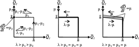
Figure 2: The fluid process that approximates the stochastic network.

First consider the case $\lambda>\mu_{1}>\mu_{2}$. A fluid model corresponding to this case is illustrated by the vector flow diagram in the left part of Figure 2. This diagram indicates the rate of change of the vector of queue lengths as a function of its value. For instance, if the two queue lengths are between 0 and $\bar{h}$, then fluid enters queue 1 at rate $\lambda$ and flows from that queue to queue 2 at rate $\mu_{1}$ while fluid leaves queue 2 at rate $\mu_{2}$. Accordingly, the length of queue 1 increases at rate $\lambda-\mu_{1}$ and that of queue 2 at rate $\mu_{1}-\mu_{2}$. The other cases can be understood similarly. The vector flow diagram shows that, irrespective of their initial values, the queue lengths converge to the pair of values $(0,\bar{h})$, which is an absorbing state for the fluid process. Moreover, when the process is close to the value $(0,\bar{h})$, the rate of the departure fluid is close to $\mu_{2}$. To conclude that the stochastic network has a departure rate close to $\mu_{2}$ when $h$ is large, one notes that the fluid process has one additional property: the time the process takes to reach the state $(0,\bar{h})$ is bounded by a linear function of the distance between the initial condition and $(0,\bar{h})$. This property, which can be seen from the vector flow diagram, can be used to show, roughly, that the stochastic system spends little time far from $(0,\bar{h})$. The intuition is that, although fluctuations occasionally move the stochastic network away from the limiting state, the system tends to follow the fluid process and get back to that state fairly quickly. This property will allow us to construct a proof that the stochastic network has a departure rate close to $\mu_{2}$ most of the time.

It turns out that one needs a generalization of the above approach to cover some interesting cases. To illustrate this generalization, consider once again the network of Figure 1, but assume that $\lambda>\mu_{1}=\mu_{2}=\mu$. The vector flow diagram of the corresponding fluid process is shown in the middle part of Figure 2. The diagram shows that the fluid process converges to some point in the set indicated by the two thicker lines: $\{\bar{h}\}\times[0,\bar{h}]\cup[0,\bar{h}]\times\{\bar{h}\}$, depending on the initial condition. While it is true that the rate of the departure fluid is close to $\mu$ for any point close to that set, it is no longer the case that the time to reach that limiting set is bounded by a linear function of the initial distance to the set. For instance, if the initial state of the fluid process is $(\bar{h},\bar{h}+\epsilon)$ for some arbitrary $\epsilon>0$, the process takes at least $\bar{h}/\mu$ to reach the limiting set. To handle this situation, one considers the set shown in the right-hand part of Figure 2. That set has the following two key properties: (1) the departure flow rate is almost $\mu$ close to that set, and (2) the time to reach the set is bounded by a linear function of the initial distance to it, as can be see from the diagram. Thus, as in the previous example, one can show that the stochastic network has a departure rate close to $\mu$ most of the time.

The main technical contributions of the paper are as follows:

• A technique for scaling time, space and threshold for finding a fluid limit for a stochastic network with threshold based ingress discarding such as in our example;

• Proof of a fluid limit for stochastic networks with thinned processes such as $\Lambda(t)$ in Figure 1;

• Proof of approximation of the rates of the stochastic network by the rates of the limiting fluid process under the two key properties indicated in our examples.

In the next subsection, we outline the key steps of our analysis. In Section 1.2 we relate our work to other prior work, and in Section 1.3 we review an example stochastic network with ingress discarding. Section 2 establishes the notation and initial model description, while Section 3 proves the main results of the article. In Section 4 we study the fluid model of a network resembling a $2\times 2$ network switch and show that the fluid model has the necessary properties to employ the main results of the article. Note that Musacchio MusacchioPhD shows that a more general network with ingress discarding has a fluid model with the necessary properties. Section 5 concludes the paper.

1.1 Proof outline

Our goal is to show that the long-term average flow rates of the stochastic system can be made arbitrarily close to a vector of desired rates $R$ if the discarding thresholds are made large enough. Moreover, we want to show that certain properties of the system’s fluid model suffice to reach this conclusion. In this subsection we outline the arguments detailed in the rest of the paper.

The queuing network we consider has ingress discarding thresholds of $nh$ in each queue, where $h>0$, and $n>0$ is a threshold scale factor that is increased to make the thresholds larger. The network is described by a Markov process $X^{n}=\{X^{n}(t),t\geq 0\}$ taking values in the state space $\mathsf{X}$. The superscript emphasizes the dependence on $n$. The state of the Markov process includes the queue lengths, remaining service times at each queue and the remaining time until the next exogenous arrival of each flow $f\in{1,\ldots,F}$. We will argue that $X^{n}$ satisfies the strong Markov property.

As we discussed in the previous section, we construct fluid limits of the system by scaling time, space and threshold scale factor in particular ways that we describe below. These fluid limits converge (in a sense also described below) to trajectories of a fluid model. The fluid model, like the original system, also has ingress discarding thresholds. However, these thresholds need not equal $h$, since one of the fluid limits we need to consider can scale space and threshold at different rates. Therefore when referring to the system’s fluid model, we need to specify $\bar{h}$, the discarding thresholds of each queue of the fluid model. (The queues of the fluid model have a common threshold $\bar{h}$, just as the queues of the original system have a common threshold $nh$.) The fluid model has a state space $\bar{\mathsf{X}}$ similar to that of the original system, but the queue lengths take values in $\mathbb{R}^{+}$ rather than $\mathbb{Z}^{+}$. In what follows we adopt the notation that if $\mathcal{S}\subset\bar{\mathsf{X}}$, then the set $a\mathcal{S}$ ($a\in\mathbb{R}_{+}$) denotes a “scaled” set such that $\bar{x}\in a\mathcal{S}$ iff $\bar{x}/a\in\mathcal{S}$. Also let $\|\bar{x}\|_{\mathcal{S}}=\inf_{e\in\mathcal{S}}\|\bar{x}-e\|$ denote the distance between $\bar{x}$ and the set $\mathcal{S}$.

Our goal is to show that if there exists a closed, bounded set $\mathcal{E}\subset\bar{\mathsf{X}}$ and $t_{0}\in\mathbb{R}^{+}$ such that conditions (C1) and (C2) below hold, then there exists a large enough $n$ such that the stochastic network achieves long-term average departure rates arbitrarily close to $R$. Conditions (C1) and (C2) are as follows:[(C2)]

All trajectories of the fluid model with ingress discarding thresholds $\bar{h}$ and initial condition $\bar{X}(0)=\bar{x}$ are absorbed by a set $\bar{h}\mathcal{E}$ in a time not more than $t_{0}\|\bar{x}\|_{\bar{h}\mathcal{E}}$;

If $\bar{h}>0$, the instantaneous departure rates of the fluid model while its state is in the set $\bar{h}\mathcal{E}$ are equal to the vector of desired rates $R$. Note that (C1) requires that $\bar{h}\mathcal{E}$ be an absorbing set of the fluid model with thresholds $\bar{h}$. For example, one can show that a minimal absorbing set of the fluid model in many cases would be, roughly, the set of states such that at least one of each flow’s set of “bottleneck” queues is at it’s discarding threshold, and servers with a utilization below 1 have empty queues. (By “bottleneck queue,” we mean a queue whose service constrains a flow’s rate in the fluid model.) However, such a construction might not be sufficient to satisfy (C1), particularly when flows do not have unique “bottlenecks.” Recall that in the Introduction we studied an example with two serially-connected queues with the same service rate. This is an example in which $\bar{h}\mathcal{E}$ needs to be made larger than the minimal absorbing set in order to satisfy (C1). To see this note that even though the two line segments in the middle panel of Figure 2 constitute an absorbing set for the fluid model, if we defined $\mathcal{E}$ so that $\bar{h}\mathcal{E}$ is equal to these two line segments (by making $\mathcal{E}=\{1\}\times[0,1]\cup[0,1]\times\{1\}$), condition (C1) would not be met. By defining $\mathcal{E}$ in such a way as to make $\bar{h}\mathcal{E}$ have the shape indicated by the shaded area of the right panel of Figure 2, the time it takes trajectories of the fluid model to reach $\bar{h}\mathcal{E}$ can be upper bounded by an amount proportional to the distance of the starting point of the trajectory from $\bar{h}\mathcal{E}$, thus satisfying (C1).

The proof depends on two main steps: [(ii)]

The expected flow rates associated with the process $X^{n}(\cdot)$, over a finite time interval of length $nt_{0}$, and for initial conditions near a set $nh\mathcal{E}$, can be made to be arbitrarily close to $R$ with a sufficiently large threshold scaling factor $n$.

The excursions of the process $X^{n}(\cdot)$ away from $nh\mathcal{E}$ become relatively shorter with larger threshold scaling factor $n$. More precisely, the first hitting time that occurs $nt_{0}$ after having started in a neighborhood of the set $nh\mathcal{E}$, can be made to be arbitrarily close to $nt_{0}$.

In both steps we make use of the fact that a fluid limit of the process $X^{n}(\cdot)$ converges to a trajectory of the fluid model, but the different objectives of the two steps require us to use different fluid limit scalings. In the first step we consider a sequence of (initial condition, scale factor) pairs $\{(x_{j},n_{j})\}$. To emphasize the dependence on initial condition and threshold scale factor we write $X^{\mathbf{x}_{j}}(\cdot)$, where the superscript ${{\mathbf{x}}_{j}}\triangleq(x_{j},n_{j})$. We require that the sequence has the properties that $x_{j}/n_{j}$ is no more than a distance $\zeta<1$ away from the set $h\mathcal{E}$, and $n_{j}\rightarrow\infty$. Otherwise, the sequence is arbitrary. We call such a sequence a near fluid limit sequence. (Equivalently, the near fluid limit condition has $\|x_{j}\|_{n_{j}h\mathcal{E}}<n_{j}\zeta$ and $n_{j}\rightarrow\infty$. In general it is often more intuitive to consider the distance of $X/n$ from the set $h\mathcal{E}$ than to consider the distance of $X$ from $nh\mathcal{E}$, so we will use whichever construction is more convenient or intuitive for the context.) We demonstrate that the sequence of scaled processes $\{\frac{1}{n_{j}}X^{\mathbf{x}_{j}}(n_{j}\cdot)\}$ converges along a subsequence, uniformly over compact time intervals, to a fluid model trajectory $\bar{X}(\cdot)$. The result largely follows from the fact that the process describing the cumulative time each server in the network is busy is Lipschitz continuous, and a sequence of Lipschitz continuous functions on a compact set converges along a subsequence. Consequently, the convergence to a fluid trajectory only holds on a finite time interval. The thresholds of the fluid model that $\bar{X}(\cdot)$ satisfies are of size $\bar{h}=h$. This is because we scale both space and threshold by the same amount in this fluid limit, so the two scalings cancel out. Moreover, the restrictions we put on the near fluid limit sequence ensure that the initial condition of the fluid model trajectory $\bar{X}(\cdot)$ is within a distance of $\zeta$ of $\bar{h}\mathcal{E}$. Thus, the fluid model trajectory $\bar{X}(t)$ hits $\bar{h}\mathcal{E}$ quickly [in not more than time $\zeta t_{0}$ by (C1)] and then achieves flow rates of $R$ [by condition (C2)].

At this point, we have only shown convergence along a subsequence to a fluid trajectory with some desired properties. We need to show convergence along the original near fluid limit sequence in order to eventually make conclusions about the stochastic network. To that end, consider a functional $\mathfrak{F}$ that extracts the difference between the actual flow throughput and the desired flow throughput over a compact time interval $[\zeta t_{0},t_{0}]$ (in time scaled by $n$). Since $\bar{X}(t)$ hits $\bar{h}\mathcal{E}$ by time $\zeta t_{0}$, the flow rates are equal to the desired rates over $[\zeta t_{0},t_{0}]$. Consequently, $\mathfrak{F}\circ\bar{X}=0$. This in turn allows us to argue that $\{\mathfrak{F}\circ\frac{1}{n}X^{\mathbf{x}_{j}}(n\cdot)\}$ converges to 0 along a subsequence. Since every near fluid limit sequence of processes (with the functional applied to them) converges along a subsequence to 0 in this way, it must be that every near fluid limit sequence also converges to 0 in this way. This fact allows us to show that the flow rates of the process $\frac{1}{n}X(n\cdot)$ can be made arbitrarily close the desired rates, for a finite time period, from any scaled initial condition $x/n$ near $h\mathcal{E}$, provided that $n$ is sufficiently large. In the detailed proof the functionals we consider act on the Markov state trajectory combined with the trajectories of some other associated processes such as the cumulative service time process. The fact that $\zeta<1$ was chosen otherwise arbitrarily is important because it allows us to later make $\zeta$ small so that the desired rates are achieved over most of the interval $[0,t_{0}]$ (in scaled time).

In the second step, we again consider a sequence of (initial condition, scale factor) pairs $\{(x_{j},n_{j})\}$. This sequence must satisfy the properties that the distance between $x_{j}/n$ and $h\mathcal{E}$ is more than a constant $\zeta$ for each $j$, and that $\|x_{j}\|_{n_{j}h\mathcal{E}}=n_{j}\|x_{j}/n_{j}\|_{h\mathcal{E}}\rightarrow\infty$. Otherwise, the sequence is arbitrary. We call such a sequence a far fluid limit sequence. We show that the sequence of scaled processes $\{X^{\mathbf{x}_{j}}(\|x_{j}\|_{n_{j}h\mathcal{E}}\cdot)/\|x_{j}\|_{n_{j}h\mathcal{E}}\}$ converges along a subsequence of any far fluid limit sequence, uniformly over compact time intervals, to a fluid model trajectory $\bar{X}(\cdot)$ satisfying a fluid model with discarding thresholds $\bar{h}$. The scaled threshold sequence of the fluid limit is $\{n_{j}h/(n_{j}\|x_{j}/n_{j}\|_{h\mathcal{E}})\}$, so the choice of sequence and convergent subsequence determines a value for $\bar{h}$ that satisfies $\bar{h}\in[0,h\zeta^{-1}]$. Also the scaling of the far fluid limit sequence ensures that the initial condition of the fluid trajectory have an initial condition that is unit distance from $\bar{h}\mathcal{E}$. This fact along with our starting assumption (C1), ensure that $\|\bar{X}(t_{0})\|_{\bar{h}\mathcal{E}}=0$. The preceding two facts allow us to argue that the sequence $\{X^{\mathbf{x}_{j}}(\|x_{j}\|_{n_{j}h\mathcal{E}}t_{0})/\|x_{j}\|_{n_{j}h\mathcal{E}}\}$ has a distance from $n_{j}h\mathcal{E}$ that converges to 0 along a subsequence. Moreover since any far fluid limit sequence has a subsequence that converges to 0 in this sense, it must be that this convergence property holds for any far fluid limit sequence.

This fact is the basis for constructing an argument that

$$\mathrm{E}\bigl{\|}X^{{\mathbf{x}}}\bigl{(}t_{0}\|x\|_{nh\mathcal{E}}\bigr{)}\bigr{\|}_{nh\mathcal{E}}\leq\delta\|x\|_{nh\mathcal{E}}$$

for any $\delta>0$ provided that threshold scale factor $n$ is sufficiently large and $\|x/n\|_{h\mathcal{E}}>\zeta$ (equivalently $\|x\|_{nh\mathcal{E}}>n\zeta$). This relation serves as a Lyapunov function which allows the construction of an argument about the recurrence time of the scaled process $X/n$ to a neighborhood with distance $\zeta$ of $h\mathcal{E}$, and this in turn allows us to conclude (ii) above.

This recurrence time argument is adapted from MeynTweedie while the overall argument we make with the far fluid limit sequence parallels Dai95 . The main difference between our far fluid limit argument and that of Dai95 is that in Dai95 the fluid model and stochastic network are drawn to the origin and neighborhood of the origin, respectively, whereas in our model the system is attracted to a set of states.

1.2 Relation to prior work

Our fluid limit proof techniques borrow heavily from work by Dai Dai95 . Dai shows that for networks without discarding, stability of a corresponding fluid model implies positive Harris recurrence of the stochastic network. In our work we use the fluid model not only to show positive Harris recurrence of the stochastic network, but also to find its long term average flow rates. Specifically, we use two fluid limits: the far fluid limit and the near fluid limit that correspond to different sequences of initial conditions and threshold pairs.

Dai’s proof considers a sequence of initial states $\{x\}$ of the Markov process describing the network, with $|x|\rightarrow\infty$, and then obtains a fluid limit by scaling time and space by $|x|$. Dai uses this result to construct a Lyapunov function to show that the expected state of the system contracts, for initial states far enough from the origin. Our far fluid limit analysis parallels this, but with the difference that our analysis focuses on the distance of the state from a set of states $h\mathcal{E}$ rather than the distance from the origin. Also, because we are interested in showing the existence of a sufficiently large threshold scaling factor $n$, for both the near and far fluid limits, we consider a sequence of initial condition threshold pairs $\{x,n\}$ to obtain our results rather than just a sequence of initial conditions as in Dai95 .

Our fluid limit technique is also very similar to that found in work by Bramson Bramson . In much the way we do, Bramson takes the fluid limit using a sequence of pairs, one being the initial condition and the other being a time scaling factor of both space and time. However, our results do not follow immediately from the results of Bramson because we require that the fluid model be drawn toward a set $\bar{h}\mathcal{E}$ rather than just to the origin.

Another body of work uses fluid limits to show rate stability rather than showing that the system state converges to an invariant distribution, or more precisely that the system is positive Harris recurrent. Rate stability means that the long-term average departures match the long-term average arrivals. It is a weaker concept than positive Harris recurrence because a system can be rate stable while internally the average queue lengths grow unbounded or at least fail to converge to an invariant distribution. For a treatment see ElTaha99 , and examples of its application include Chen95 and Dai00 . The rate stability framework is not sufficient for our objectives because in order to show that our control policy achieves flow rates close to those predicted by a fluid model, we need to show that the vector of queue lengths settles to an invariant distribution concentrated near a particular set of lengths, as illustrated in the example of the Introduction.

Another closely related work to ours is by Mandelbaum, Massey and Reiman Mandelbaum . In Mandelbaum , the authors study the fluid limit of a queueing network with state dependent routing, where the function describing the arrivals to each queue can scale with $n$ and or $\sqrt{n}$, in a manner similar to the scaling of our thresholds. The authors prove a functional strong law of large numbers and a functional central limit theorem in the context of their model. However, the authors assume that the network is driven by Poisson processes, rather than just the renewal assumption that we make. An earlier work by Konstantopoulos, Papadakis and Walrand derives a functional strong law of large numbers and a functional central limit theorem for networks with state dependent service rates Takis .

There are also several other works that use reflected Brownian motion models to study queueing networks with blocking DaiHarrison , Harrisonbook , harrisonrbm . Typically the objective of most such investigations is to approximate the distribution of the queue occupancy with a diffusion approximation. In contrast with those works, our objective is to show almost sure convergence using a strong law of large numbers scaling.

1.3 Example network

In this subsection, we introduce an example that motivates the theory developed in this paper. The example will illustrate two important phenomena—that the long-term rates of the stochastic system get closer to those of a corresponding fluid model when discarding thresholds are raised, and that when there are not unique bottlenecks, the vector of queue depths is not attracted to a unique equilibrium point.

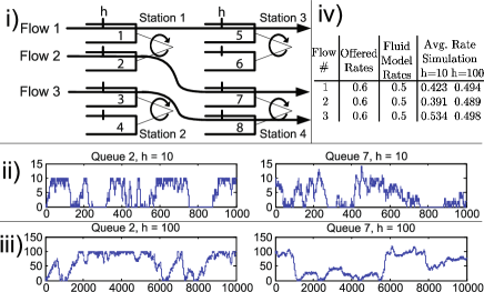
Figure 3: (i) An illustration of the example network. (ii) The queue lengths of queue 2 and 7 when the discarding threshold parameter $h$ set to $10$. (iii) The lengths of queue 2 and 7 when the discarding threshold parameter $h$ is set to $100$. (iv) The average flow rates of each of the three flows for both the $h=10$ and $h=100$ simulated sample paths.

Our example is illustrated in Figure 3. The example is analogous to a two-input and two-output switch. Two flows enter the network at station 1, the first input of the switch, and a third flow enters the network at station 2. We concentrate on flow 2, which shares stations 1 and 4 with flows 1 and 3, respectively. All stations are served at rate 1, have round-robin service with equal weighting to all queues, and have service times that are exponentially distributed. The arrival rate of each flow is 0.6, with Pareto inter-arrival distributions given by

$$\mathrm{P}\bigl{(}\xi_{f}(j)>s\bigr{)}=\frac{1}{(0.6s+1)^{2}},\qquad f\in\{1,2,3\},s\geq 0,$$

where $\xi_{f}(j)$ is the inter-arrival time preceding the $j$th arrival. We choose the Pareto distribution for this example to emphasize that we are interested in networks whose inter-arrival and service times are not necessarily memoryless.

We consider the behavior of the network’s fluid model. Since stations 2 and 3 have a capacity of 1 and each carry one flow with an offered rate of 0.6, the queues of these stations should never fill. Stations 1 and 4 each carry 2 flows that offer a load of 0.6 (before considering discarding). The fluid model of the station’s round robin service is that each station serves both of its queues at rate 0.5 as long as both flows are offering enough customers to be served at this rate. Consequently, when flow 1’s queue at station 1 is filled below threshold, this queue grows at a rate of 0.1. However, if flow 1’s queue at station 1 ever went above its threshold, ingress discarding would commence, and the queue would immediately decrease. Therefore, it must be that this queue grows to its threshold, stays at this level and then flow 1’s “thinned” or post-discarding arrival process is of rate 0.5.

Similar reasoning shows that flow 3’s queue at station 4 behaves in this way, and also that one of flow 2’s queues must also reach the threshold and “stick” there. These steps allow us to conclude that after some time, all three flows should have rates of 0.5 in the system’s fluid model. (We will verify this carefully in Section 4.)

Figure 3 shows the simulated trajectories of flow 2’s queues at both bottleneck stations in the stochastic network. In the $h=10$ case, the simulation shows that queues 2 and queue 7, which both serve flow 2, are empty for over 100 time units around time 800. This empty period is significant because when flow 2’s queues are empty, flow 2 misses opportunities to have its customers served by the bottleneck stations. Indeed the table included in Figure 3 shows the average rate, averaged over the last $80\%$ of the simulation time to reduce some of the initial transient effect, is $0.391$. This is substantially below the rate of $0.5$ predicted by the fluid model. Most likely, a string of long interarrival times of flow $2$, caused the queues at the bottleneck stations to starve.

Raising the thresholds should reduce starvation, because larger thresholds would provide the bottleneck queues a larger backlog to smooth over fluctuations in the arrival and service processes. To test that intuition, we simulate the network with discarding thresholds of $h=100$. Figure 3 shows the trajectories of flow 2’s queues for the increased threshold. We note that neither queue spends all of the time filled to its threshold, but instead at most times at least one of the queues is near its threshold. For instance, at the beginning of the simulation, queue 7 (the second bottleneck) is chattering near the threshold while queue 2 (the first bottleneck) is below threshold. At some time before the 2000 second mark, the two queues switch these roles, and around the 6000 second mark the queues switch these roles again. We also note that flow 2 achieves an average rate of $0.489$, which is much closer to the rate of $0.5$ predicted by the fluid model.

2 Preliminaries

Customers of a given flow $f\in\{1,\ldots,F\}$ follow the same fixed sequence of distinct stations. The service times are independent. Each flow $f$ has a weight $w_{f}$ and each station $i\in\{1,\ldots,d\}$ is equipped with per-flow queues and serves each flow in proportion to its weight using a weighted round robin or a similar queueing discipline. In addition to the notion of flow, each customer also has a class $k\in\{1,\ldots,K\}$ that is indicative of both the customer’s flow and the station $s(k)$ it is located. Thus the class of a flow $f$ customer changes as the customer progresses from station to station, but with the restriction that a flow $f$ customer must always have a class in the set $K(f)$. Conversely, each class $k$ is associated with one and only one flow $\mathrm{f}_{(k)}$. We also adopt the numbering convention that flow $f$ customers enter the network as class $k=f$, and thus $f\in K(f)$. The constituency matrix $C\in\{0,1\}^{d\times K}$ records which classes are served in each station: $C_{ik}=1$ if class $k$ is served at station $i$, otherwise $C_{ik}=0$. A customer of class $k$ who completes service becomes a customer of class $l$ if $P_{kl}=1$. Thus $P\in\{0,1\}^{K\times K}$ is a binary incidence matrix with each row containing at most one 1. Because flows follow loop-free paths, $P$ is nilpotent.

The exogenous arrivals to the network for flow $f$ are described by a renewal process $E_{f}(\cdot)$ for which the interarrival times $\{\xi_{f}(j),j\geq 1\}$ are i.i.d. and $\alpha_{f}$ is the mean arrival rate. Thus,

$$E_{f}(t)=\max\bigl{\{}r\dvtx U_{f}(0)+\xi_{f}(1)+\cdots+\xi_{f}(r-1)\leq t\bigr{\}},\qquad t\geq 0,$$

where $U_{f}(t)\in\mathbb{R}_{+}$ is the time after time $t$ until the next flow $f$ customer arrives at the network ingress. We also need to assume that inter-arrival times are unbounded and spread-out. More precisely, we assume that for each $k\in\{0,\ldots,F\}$, there exists an integer $j_{k}$ and some function $p_{k}(x)\geq 0$ on $\mathbb{R}^{+}$ with $\int_{0}^{\infty}p_{k}(x)\,dx>0$, such that

$$\mathrm{P}\bigl{[}\xi_{k}(1)\geq x\bigr{]}>0\qquad\mbox{for any }x>0$$ (1)

and

$$\mathrm{P}\Biggl{[}a\leq\sum_{i=1}^{j_{k}}\xi_{k}(i)\leq b\Biggr{]}\geq\int_{a}^{b}p_{k}(x)\,dx\qquad\mbox{for any }0\leq a\leq b.$$ (2)

The service times $\{\eta_{k}(j),j\geq 1\}$ of each class $k$ are also i.i.d. and have mean $m_{k}=\mu_{k}^{-1}$, where $\mu_{k}$ is the mean service rate. We also define the $K\times K$ diagonal matrix $M$ whose $k$th diagonal entry is $m_{k}$. The quantity $V_{k}(t)\in\mathbb{R}_{+}$ denotes the remaining service time of the class $k$ customer in service, if there is one at time $t$, otherwise $V_{k}(t)=0$. We define a service process $S^{\mathbf{x}}_{k}(\cdot)$ as

$$S_{k}(t)\triangleq\max\bigl{\{}j\dvtx\tilde{V}_{k}(0)+\eta_{k}(1)+\cdots+\eta_{k}(j-1)\leq t\bigr{\}},\qquad t\geq 0,$$

where $\tilde{V}_{k}(0)=V_{k}(0)$ if $V_{k}(0)>0$; otherwise $\tilde{V}_{k}(0)=\eta_{k}(0)$ is a fresh service time with the same distribution as $\eta_{k}(1)$ and independent of all other service times.

In principle, our assumption that the service times are independent does not allow for service times that depend on a packet’s size (taking “packets” to be “customers”). Dependence on packet size would make the service times of stations dependent on each other. To model this explicitly would require a much more complicated model. However we believe that our results in this work would still hold if this assumption were relaxed.

We define the following right-continuous processes: $A\dvtx[0,\infty)\rightarrow\mathbb{Z}_{+}^{K}$ counts the arrivals to each class $k$ since time $t=0$; $D\dvtx[0,\infty)\rightarrow\mathbb{Z}_{+}^{K}$ counts the departures of each class; $\Lambda\dvtx[0,\infty)\rightarrow\mathbb{Z}_{+}^{F}$, counts the exogenous arrivals of each flow that make it past the discarding point (“thinned” exogenous arrivals); $Q\dvtx[0,\infty)\rightarrow\mathbb{Z}_{+}^{K}$ is the vector process of queue depths; $T\dvtx[0,\infty)\rightarrow\mathbb{R}_{+}^{K}$ counts the total time each class $k$ has been served since $t=0$; and $I\dvtx[0,\infty)\rightarrow\mathbb{R}_{+}^{d}$ counts the total time each server has been idle since $t=0$. For each $t\geq 0$, these processes satisfy the following relations:

$$\displaystyle A(t)=P^{T}D(t)+\Lambda(t);$$ (3)

$$\displaystyle Q(t)=Q(0)+A(t)-D(t);$$ (4)

$$\displaystyle Q(t)\geq 0;$$ (5)

$$\displaystyle T_{k}(t)\mbox{ is nondecreasing and }T_{k}(0)=0\qquad\mbox{for $k=1,\ldots,K$};$$ (6)

$$\displaystyle I_{i}(t)=t-C_{i}T(t)\mbox{ is nondecreasing and }I_{i}(0)=0\qquad\mbox{for $i=1,\ldots,d$};$$ (7)

$$\displaystyle\int_{0}^{\infty}\bigl{(}CQ(t)\bigr{)}\,dI(t)=0;$$ (8)

$$\displaystyle D_{k}(t)=S_{k}\bigl{(}T_{k}(t)\bigr{)}\qquad\mbox{for $k=1,\ldots,K$}.$$ (9)

Relations (3)–(5) describe the relations between the arrival, departure and queue length processes. Statements (6)–(8) describe basic restrictions on the cumulative service time and idle time processes, with relation (8) reflecting an assumption that each station is work conserving. Equation (9) reflects that departures of class $k$ are determined by the composition of the service time counting process $S_{k}(\cdot)$ and the process $T(\cdot)$.

The ingress discarding scheme drops arriving customers of flow $f$ as they arrive whenever any queue in the set $K(f)$ exceeds a high threshold $nh$. Recall that $n$ is the threshold scaling factor which we will adjust in our analysis. Conversely, when all of the queues in $K(f)$ are below a lower threshold $nh-o(n)$, flow $f$ customers are permitted to enter the network. Note the lower threshold could be set to be the same as the upper threshold, but in some practical applications it might be beneficial to have different thresholds so that the switching between admitting and discarding is less frequent. Thus we permit this difference between upper and lower thresholds to be any function $o(n)$ that satisfies $o(n)/n\rightarrow 0$ and $o(n)\geq 0$. For instance any nonnegative constant may be used. Between these thresholds, the system has hysteresis behavior, and we define this behavior as follows. A process $H_{k}\dvtx[0,\infty)\rightarrow\{0,1\}$ keeps track of whether discarding has been “turned-on” by each class $k$ queue. If $Q_{k}(t)\geq nh$, then $H_{k}(t)=1$, and if $Q_{k}(t)\leq nh-o(h)$, then $H_{k}(t)=0$. For all $t$ such that $Q_{k}(t)\in(nh-o(h),nh)$, the evolution of $H_{k}$ is determined by the following rules:

• If $H_{k}(t)=0$, then let $t_{s}=\min\{\tau\geq 0\dvtx Q_{k}(t+\tau)\geq nh\}$ [note that $t_{s}$ is well defined because $Q_{k}(\cdot)$ is right continuous]. $H_{k}(t+\tau)=0$ for $\tau\in[0,t_{s})$ and $H_{k}(t_{s})=1$.

• If $H_{k}(t)=1$, then let $t_{s}=\min\{\tau\geq 0\dvtx Q_{k}(t+\tau)<nh-o(n)\}$. $H_{k}(t+\tau)=1$ for $\tau\in[0,t_{s})$ and $H_{k}(t_{s})=0$.

The flow $f$ customers that are allowed into the network beyond the discarding point depends on all the processes $H_{k}(\cdot)$ as

$$\Lambda_{f}(t)=\sum_{j=1}^{E_{f}(t)}\prod_{K(f)}\bigl{(}1-H_{k}(\tau_{j}-)\bigr{)},$$ (10)

where $\tau_{j}=U_{f}(0)+\sum_{m=1}^{j-1}\xi_{f}(m)$ is the time of the $j$th arrival to the discarding point. Here the dependence on $H_{k}(\tau_{j}-)\triangleq\lim_{t\uparrow\tau_{j}}H_{k}(t)$ rather than $H_{k}(\tau_{j})$ is to avoid problems with causality. For instance a customer arrival that triggers discarding should not be discarded; otherwise the customer will never arrive to the system, and paradoxically the discarding will never turn on. Our modeling choice allows such a customer to enter, thus triggering discarding, which will discard future customers.

The queueing discipline of a station $i$ serves each flow in proportion to the flow weights over long time intervals. More precisely, for some constant $c>0$ and all $\tau>0$,

$$\frac{D_{k}(t,t+\tau)}{w_{\mathrm{f}_{(k)}}}\geq\frac{D_{l}(t,t+\tau)}{w_{\mathrm{f}_{(l)}}}-c\qquad\mbox{whenever $Q_{k}(s)>0$ $\forall s\in[t,t+\tau]$}$$ (11)

for all $k,l\in C(i)\triangleq\{k^{\prime}\dvtx C_{ik^{\prime}}=1\}$, where $D_{k}(t,t+\tau)\triangleq D_{k}(t+\tau)-D_{k}(t)$.

We furthermore assume that only the customer at the head of line of each queue may be served, and that the instantaneous service rate of any queue is a function of the current state. That is, $\dot{T}_{k}(t)=f(X(t))$ for some function $f(\cdot)$ where $X(t)=[Q(t);U(t);V(t);H(t)]$.

The evolution of the queuing system depends on the particular queuing discipline. Moreover, some queueing disciplines require additional state variables. For instance, a weighted round robin scheduler visits the queues in a cyclic order, serving any customers at the head of the line. The order should be chosen so that in each cycle the number of visits of each queue is proportional to the flow weights (which is possible if the weights are rational multiples of each other). Other queueing disciplines could be considered as well, though these disciplines may need additional state variables. For instance, deficit round robin (DRR) requires counters for each class DRR . Also, DRR ensures that the service times given to each class are proportional rather than the number of customers served. Therefore, DRR satisfies a criterion similar to (11) except that $D(\cdot)$ is replaced by $T(\cdot)$. However, since the service times are unbounded, the criterion holds only in the limit $\tau\rightarrow\infty$, almost surely. Other disciplines require yet more complex state descriptions. For instance, weighted fair queueing (WFQ) keeps track of each customer’s “virtual finish time”—the time they would have departed if the service discipline were weighted processor sharing and no more customers were to arrive Bertsekas . To keep the presentation simple, we assume that the additional state variables required by the queueing discipline are described by a bounded vector in $\mathbb{Z}_{+}^{d}$. We append this to the $H$ portion of the state description. Treatment of queueing disciplines that require more elaborate state descriptions requires some modification to the statement and proof of Theorem 1.

2.1 State description

The dynamics of the queueing network are described by the Markov process $X=\{X(t),t\geq 0\}$. The state description contains the queue lengths $Q(t)\in\mathbb{R}_{+}^{K}$ of all the $K$ queues in the network, as well as the residual arrival and service times $U(t)\in\mathbb{R}_{+}^{F}$ and $V(t)\in R_{+}^{K}$, respectively. Recall that $U(t)$ and $V(t)$ are defined to be right-continuous. Finally the state description includes the state of the discarding hysteresis and any state variables used by the queueing discipline as described above. We assume that $H(t)\in\{0,1\}^{K}\times\mathbb{Z}_{+}^{d}$. Thus the full state description is

$$X(t)=\bigl{[}Q(t);U(t);V(t);H(t)\bigr{]}.$$

Let $\mathsf{X}\subset\mathbb{Z}^{K}\times\mathbb{R}_{+}^{F+K}\times\{0,1\}^{K}\times\mathbb{Z}_{+}^{d}$ be the set of all states $X$ can take. A fixed threshold scaling factor $n$, an initial condition $x=X(0)\in\mathsf{X}$ is sufficient to specify the statistics of the future evolution of the system.

We claim that the process $X$ satisfies the strong Markov property, by the same argument given by Dai Dai95 . In turn, Dai’s argument followed from Kaspi and Mandelbaum kaspimandelbaum . Without repeating all the details of the argument, the basic idea is that $X(\cdot)$ is a piecewise deterministic Markov (PDM) process—behaving deterministically between the generation of “fresh” inter-arrival or service time. Davis shows that a PDM process whose expected number of jumps on $[0,t]$ is finite for each $t$ is strong Markov davis . As we assume that the inter-arrival and service times have a positive and finite mean, the expected number of jumps of $X(\cdot)$ in any closed time interval is finite. Therefore $X(\cdot)$ has the strong Markov property.

The fluid model, whose defining equations will be given in Theorem 1, takes values in the state space $\bar{\mathsf{X}}\subset\mathbb{R}_{+}^{F+3K+d}$ since integer valued states of the original system correspond to real valued states of the fluid model.

3 Fluid limit analysis

In this and subsequent sections, we use the superscript ${{\mathbf{x}}}\triangleq(x,n)$ to denote the dependence on initial state $x$ and threshold scaling factor $n$. As we discussed earlier, we use two different fluid limits in our analysis: the near and far fluid limits that study behavior of the stochastic network for scaled initial conditions near and far from $h\mathcal{E}$, respectively. Recall that $\mathcal{E}\subset\bar{\mathsf{X}}$ is a closed and bounded set. Also recall $h\mathcal{E}=\{x\dvtx x/h\in\mathcal{E}\}$. At this point we make no further assumptions on $\mathcal{E}$, but eventually $\mathcal{E}$ will have to be chosen so that $\bar{h}\mathcal{E}$ is an absorbing set of the fluid model with thresholds $\bar{h}$ to apply our final results.

For notational convenience we also define an augmented state vector process

$$\mathfrak{X}^{{\mathbf{x}}}{(\cdot)}\triangleq\bigl{[}X^{\mathbf{x}}(\cdot);T^{\mathbf{x}}(\cdot);\Lambda^{\mathbf{x}}(\cdot);nh\bigr{]},$$

which contains all the functions that we want to show converging in both kinds of fluid limit.

In this section, we state Theorem 1 which shows convergence to a fluid model trajectory along a fluid limit. The convergence of the trajectory is uniformly on compact sets. More precisely, we say that $f_{j}(t)\rightarrow f(t)$ uniformly on compact sets (u.o.c.) if for each $t\geq 0$,

$$\lim_{j\rightarrow\infty}\sup_{0\leq s\leq t}\bigl{|}f_{j}(s)-f(s)\bigr{|}=0.$$

We also use the notation $\dot{f}(t)=\frac{d}{dt}f(t)$ where such a derivative exists. If a function $f(\cdot)$ is differentiable at $t$, we say that $t$ is a regular point.

The proof, along with four lemmas used in the proof, are given in the Appendix. One of these lemmas, Lemma 5, is a new result showing that the thinned arrival process converges u.o.c. to the fluid limit. In Section 1.1 we previewed the two types of fluid limits, which we call the “near” and “far” fluid limits, that we will use in our analysis. In both types of fluid limits, time and space is scaled by a factor that increases. In the development that follows, that scale factor for time and space is represented by the notation $a_{j}$. Later on, we will make specific assumptions about $a_{j}$ that correspond to either the near or far fluid limit. Bramson Bramson takes a similar approach to defining the fluid limit. Both types of fluid limit scale the threshold no faster than time and space are scaled, and also both consider a sequence of initial conditions $x_{j}$, such that after space-scaling, the “relative initial condition” $x_{j}/a_{j}$ is a bounded distance away from the set $\frac{n_{j}h}{a_{j}}\mathcal{E}$. More precisely, we define the following property which is common to both near and far fluid limit sequences. Thus by assuming this property in the statement of Theorem 1, the theorem applies to both near and far fluid limit sequences.

Property 1.

$\{({{\mathbf{x}}_{j}},a_{j})\}$ is a sequence of initial condition $x_{j}$, threshold factor $n_{j}$ and scale $a_{j}$ triples for which $a_{j}\rightarrow\infty$. Moreover for each $j$, $n_{j}>0$, $a_{j}>0$ and some closed, bounded $\mathcal{E}\in\bar{\mathrm{X}}$,

$$\frac{n_{j}}{a_{j}}\leq c_{1}\quad\mbox{and}\quad\biggl{\|}\frac{x_{j}}{a_{j}}\biggr{\|}_{{n_{j}h\mathcal{E}}/{a_{j}}}\leq c_{2}\qquad\mbox{for some }c_{1}>0\mbox{ and }c_{2}>0.$$

3.1 Convergence to a fluid limit along a subsequence

The proof of the following theorem parallels the proof of Theorem 4.1 of Dai Dai95 . However, the proof of our theorem differs in that we require some specialized treatment for our fluid limit construction and for the ingress discarding feature of the network. We state the theorem here and present the proof in the Appendix.

Theorem 1

Suppose $\{({{\mathbf{x}}_{j}},a_{j})\}$ is a sequence satisfying Property 1 (on page 1). Then for almost all $\omega$ there exists a subsequence $\{({{\mathbf{x}}_{m}},a_{m})\}\subseteq\{({{\mathbf{x}}_{j}},a_{j})\}$ for which

$$\frac{\mathfrak{X}^{{\mathbf{x}}_{m}}(a_{m}t)}{a_{m}}\rightarrow\bar{\mathfrak{X}}(t)\qquad\mbox{u.o.c.}$$

for some fluid model trajectory $\bar{\mathfrak{X}}(\cdot)$ with components

$$\bar{\mathfrak{X}}(\cdot)\triangleq\bigl{[}\bar{X}(\cdot);\bar{T}(\cdot);\bar{\Lambda}(\cdot);\bar{h}\bigr{]},$$

where, in turn, the process $\bar{X}(\cdot)$ has components

$$\bar{X}(\cdot)\triangleq\bigl{[}\bar{Q}(\cdot);\bar{U}(\cdot);\bar{V}(\cdot);\bar{H}(\cdot)\bigr{]},$$

where $\bar{H}(\cdot)\equiv 0$. The process $\bar{\mathfrak{X}}(\cdot)$ may depend upon $\omega$ and the choice of subsequence $\{({{\mathbf{x}}_{m}},a_{m})\}$ but must satisfy the following properties for all $t\geq 0$:

$$\displaystyle\bar{U}_{f}(t)=\bigl{(}t-\bar{U}_{f}(0)\bigr{)}^{+},\qquad\bar{V}_{k}(t)=\bigl{(}t-\bar{V}_{k}(0)\bigr{)}^{+};$$ (12)

$$\displaystyle\bar{T}_{k}(t)\mbox{ is nondecreasing and starts from zero};$$ (13)

$$\displaystyle\bar{I}_{i}(t):=t-C_{i}\bar{T}(t)\mbox{ is nondecreasing};$$ (14)

$$\displaystyle\bar{D}_{k}(t):=\mu_{s(k)}\bigl{(}\bar{T}_{k}(t)-\bar{V}_{k}(0)\bigr{)}^{+};$$ (15)

$$\displaystyle\bar{A}(t):=P^{\top}\bar{D}(t)+\bar{\Lambda}(t);$$ (16)

$$\displaystyle\bar{Q}(t):=\bar{Q}(0)+\bar{A}(t)-\bar{D}(t);$$ (17)

$$\displaystyle\bar{Q}(t)\geq 0;$$ (18)

$$\displaystyle\int_{0}^{\infty}\bigl{(}C\bar{Q}(t)\bigr{)}\,d\bar{I}(t)=0,$$ (19)

where (12), (13) and (15) hold for each flow $f$ and class $k$, while (14) holds for each station $i$. Assignments (14), (15), (16) and (17) define $\bar{I}(t)$, $\bar{D}(t)$, $\bar{A}(t)$ and $\bar{Q}(t)$, respectively. Also, the following hold for each flow $f$ for regular $t\geq 0$:

$$\dot{\bar{\Lambda}}_{f}(t) = 0\qquad\mbox{whenever $\bar{Q}_{k}(t)>\bar{h}$ for some $k\in\mathcal{C}(f)$},$$ (20)

$$\dot{\bar{\Lambda}}_{f}(t) = \alpha_{f}1\bigl{(}t\geq\bar{U}_{f}(0)\bigr{)}\qquad\mbox{whenever $\bar{Q}_{k}(t)<\bar{h}$ for all $k\in\mathcal{C}(f)$},$$ (21)

$$\dot{\bar{\Lambda}}_{f}(t) \leq \alpha_{f}.$$ (22)

Also, for station $i$ and for any $k,l$ such that $\{k,l\}\in C(i)$ the following properties are satisfied for all regular $t\geq 0$:

$$w_{k}^{-1}\dot{\bar{D}}_{k}(t) \geq w_{l}^{-1}\dot{\bar{D}}_{l}(t)\qquad\mbox{whenever $Q_{k}(t)>0$},$$ (23)

$$w_{k}^{-1}\dot{\bar{D}}_{k}(t) = w_{l}^{-1}\dot{\bar{D}}_{l}(t)\qquad\mbox{whenever $Q_{k}(t)>0$ and $Q_{l}(t)>0$}.$$ (24)

See the Appendix for the proof. Next we state precisely the definitions of a near fluid limit sequence and far fluid limit sequence that we discussed earlier in Section 1.1. After defining these sequences, we derive two corollaries to Theorem 1 that apply to each of these types of sequences.

Definition 1 ((Near fluid limit sequence)).

$\{({{\mathbf{x}}_{j}},a_{j})\}$ is a near fluid limit sequence with respect to a closed, bounded $h\mathcal{E}\in\bar{\mathsf{X}}$ if $a_{j}=n_{j}$, $n_{j}\rightarrow\infty$ and

$$\biggl{\|}\frac{x_{j}}{n_{j}}\biggr{\|}_{h\mathcal{E}}=\frac{\|x_{j}\|_{n_{j}h\mathcal{E}}}{n_{j}}\leq\zeta$$

for each $j$ and for some $\zeta>0$.

Definition 2 ((Far fluid limit sequence)).

$\{({{\mathbf{x}}_{j}},a_{j})\}$ is a far fluid limit sequence with respect to a closed, bounded $h\mathcal{E}\in\bar{\mathsf{X}}$ if $a_{j}=n_{j}\|\frac{x_{j}}{n_{j}}\|_{h\mathcal{E}}$, $a_{j}\rightarrow\infty$ and

$$\biggl{\|}\frac{x_{j}}{n_{j}}\biggr{\|}_{h\mathcal{E}}=\frac{\|x_{j}\|_{n_{j}h\mathcal{E}}}{n_{j}}>\zeta$$

for each $j$ and for some $\zeta>0$.

As was discussed earlier, the near fluid limit sequence is defined so that the sequence of scaled initial conditions remains a bounded distance away from the set $h\mathcal{E}$ while the far fluid limit is defined so that the sequence of scaled initial conditions is bounded away from the set $h\mathcal{E}$.

Corollary 1.

Suppose that $\{({{\mathbf{x}}_{j}},a_{j})\}$ is a near fluid limit sequence with respect to a closed, bounded $h\mathcal{E}\in\bar{\mathsf{X}}$. Then for almost all $\omega$ there exists a subsequence $\{({{\mathbf{x}}_{m}},a_{m})\}\subseteq\{({{\mathbf{x}}_{j}},a_{j})\}$ for which

$$\frac{\mathfrak{X}^{{\mathbf{x}}_{m}}(a_{m}t)}{a_{m}}\rightarrow\bar{\mathfrak{X}}(t)\qquad\mbox{u.o.c.},$$

where $\mathfrak{X}(\cdot)$ satisfies fluid model equations (12)–(24). Moreover

$$\bar{h}=h\quad\mbox{and}\quad\bigl{\|}\bar{X}(0)\bigr{\|}_{\bar{h}\mathcal{E}}\leq\zeta.$$

The discarding thresholds before scaling are $n_{j}h$, and thus after scaling they are $n_{j}h/a_{j}=h$ for each $j$. Thus $\bar{h}=h$. Also $a_{j}\rightarrow\infty$ and $\|x_{j}/a_{j}\|_{h\mathcal{E}}\leq\zeta$, and thus the sequence $\{({{\mathbf{x}}_{j}},a_{j})\}$ satisfies Property 1. By Theorem 1 there exists a subsequence $\{({{\mathbf{x}}_{m}},a_{m})\}$ such that ${\mathfrak{X}^{{\mathbf{x}}_{m}}(a_{m}t)}/{a_{m}}$ converges u.o.c. to a fluid trajectory satisfying (12)–(24). By Theorem 1, the subsequence $x_{m}/a_{m}$ converges to an initial state of the fluid trajectory $\bar{X}(0)$. Since $\|x_{m}/a_{m}\|_{h\mathcal{E}}\leq\zeta$, it must be that $\|\bar{X}(0)\|_{\bar{h}\mathcal{E}}\leq\zeta$.

Corollary 2.

Suppose that $\{({{\mathbf{x}}_{j}},a_{j})\}$ is a far fluid limit sequence with respect to a closed, bounded $h\mathcal{E}\in\bar{\mathsf{X}}$. Then for almost all $\omega$ there exists a subsequence $\{({{\mathbf{x}}_{m}},a_{m})\}\subseteq\{({{\mathbf{x}}_{j}},a_{j})\}$ for which

$$\frac{\mathfrak{X}^{{\mathbf{x}}_{m}}(a_{m}t)}{a_{m}}\rightarrow\bar{\mathfrak{X}}(t)\qquad\mbox{u.o.c.},$$

where $\mathfrak{X}(\cdot)$ satisfies fluid model equations (12)–(24). Moreover

$$\bar{h}\in[0,h/\zeta]\quad\mbox{and}\quad\bigl{\|}\bar{X}(0)\bigr{\|}_{\bar{h}\mathcal{E}}=1.$$

Note that

$$\biggl{\|}\frac{x_{j}}{a_{j}}\biggr{\|}_{{n_{j}h\mathcal{E}}/{a_{j}}}=\frac{n_{j}}{a_{j}}\biggl{\|}\frac{x_{j}}{n_{j}}\biggr{\|}_{h\mathcal{E}}=1$$

for each $j$. This combined with the fact that $a_{j}\rightarrow\infty$ implies that $\{({{\mathbf{x}}_{j}},a_{j})\}$ satisfies Property 1. By Theorem 1 there exists a subsequence $\{({{\mathbf{x}}_{m}},a_{m})\}$ such that ${\mathfrak{X}^{{\mathbf{x}}_{m}}(a_{m}t)}/{a_{m}}$ converges u.o.c. to a fluid trajectory satisfying (12)–(24). The above equation also implies that $\|\bar{X}(0)\|_{\bar{h}\mathcal{E}}=1$. The subsequence of scaled thresholds satisfies $n_{m}h/a_{m}=h/\|{x_{m}}/{n_{m}}\|_{h\mathcal{E}}<h/\zeta$. By Theorem 1 the subsequence $n_{m}h/a_{m}$ converges, and the convergence must be to a number in the range $[0,h/\zeta]$ because of the preceding inequality relation.

3.2 Convergence along subsequences to convergence along sequences

In the previous section, we showed that for both near and far fluid limit sequences, we can extract a sample path dependent subsequence that converges to a fluid model trajectory. The objective of this section is to use this subsequence result to show convergence of a functional of the original sequence. In particular, we show in Lemma 1 that if a functional $\mathfrak{F}$ of any fluid model trajectory goes to zero in a time not more than a constant times the scaled initial condition’s distance from $\bar{h}\mathcal{E}$, then the value of that functional applied to the fluid limit sequence of trajectories converges almost surely. In later sections, we will invoke Lemma 1 choosing $\mathfrak{F}$ to extract the service rates from the fluid model, and later choosing $\mathfrak{F}$ to extract the distance from a set $h\mathcal{E}$. Lemma 1 is a generalization of an argument used by Dai in the proof of Theorem 4.2 of Dai95 .

Lemma 1

Suppose that $\mathfrak{F}$ is a functional that maps $\mathbb{R}^{r}\times\mathbb{R}^{+}$ into $\mathbb{R}^{s}\times\mathbb{R}^{+}$ where $r$ is the dimension of $\mathfrak{X}^{\mathbf{x}}(\cdot)$ and $s$ is arbitrary. Also suppose that $\mathfrak{F}$ is continuous on the topology of uniform convergence on compact sets. If the following is true:

• The fluid model equations (12)–(24) are such that for any trajectory $\bar{\mathfrak{X}}(\cdot)$ and $\bar{h}\geq 0$ that satisfies them, there exists some closed bounded $\mathcal{E}\in\bar{\mathsf{X}}$ for which

  $$\mathfrak{F}\circ\bigl{[}\bar{\mathfrak{X}}(\cdot)\bigr{]}(t)\equiv 0\qquad\forall t\geq t_{0}\bigl{\|}\bar{X}(0)\bigr{\|}_{\bar{h}\mathcal{E}}.$$ (25)

Then, for any sequence $\{({{\mathbf{x}}_{j}},a_{j})\}$ satisfying Property 1 where the relation $\|x_{j}/a_{j}\|_{{n_{j}h\mathcal{E}}/{a_{j}}}\leq c$ of Property 1 is satisfied with constant $c>0$,

$$\biggl{|}\mathfrak{F}\circ\biggl{[}\frac{1}{a_{j}}\mathfrak{X}^{{\mathbf{x}}_{j}}(a_{j}\cdot)\biggr{]}(t)\biggr{|}\rightarrow 0\qquad\mbox{a.s.}$$ (26)

for each $t\geq ct_{0}$.

By Theorem 1, for almost all sample paths $\omega$, and for any subsequence $\{({{\mathbf{x}}_{m}},a_{m})\}\subseteq\{({{\mathbf{x}}_{j}},a_{j})\}$ there is a sample-path-dependent further-subsequence $\{({{\mathbf{x}}_{r(\omega)}},a_{r(\omega)})\}\subseteq\{({{\mathbf{x}}_{m}},a_{m})\}$ for which

$$\frac{\mathfrak{X}^{{\mathbf{x}}_{r(\omega)}}(a_{r(\omega)}t,\omega)}{a_{r(\omega)}}\rightarrow\bar{\mathfrak{X}}(t,\omega)\qquad\mbox{u.o.c.},$$

where $\bar{\mathfrak{X}}(t,\omega)$ satisfies (12)–(24) as well as $\|\bar{X}(0)\|_{\bar{h}\mathcal{E}}\leq c$ since each $x_{j}/a_{j}$ has a distance from $\frac{n_{j}h}{a_{j}}\mathcal{E}$ that is no more than $c$ by the lemma’s assumption. The notation $r(\omega)$ and $\bar{\mathfrak{X}}(t,\omega)$ emphasize that the further-subsequence and fluid trajectory depend on $\omega$. Now fix an $\omega$ for which subsequences have convergent further subsequences as described. For the next few steps we suppress the $\omega$ arguments to simplify notation. Because $\mathfrak{F}$ is assumed to be continuous on the topology of uniform convergence on compact sets, we have

$$\mathfrak{F}\circ\biggl{[}\mbox{$\frac{\mathfrak{X}^{{\mathbf{x}}_{r}}(a_{r}\cdot)}{a_{r}}$}\biggr{]}(t)\rightarrow\mathfrak{F}\circ\bigl{[}\bar{\mathfrak{X}}(\cdot)\bigr{]}(t)\qquad\mbox{u.o.c.}$$

Consequently,

$$\biggl{|}\mathfrak{F}\circ\biggl{[}\mbox{$\frac{\mathfrak{X}^{{\mathbf{x}}_{r}}(a_{r}\cdot)}{a_{r}}$}\biggr{]}(t)\biggr{|}\rightarrow 0$$

for each $t\geq ct_{0}$. So for this fixed $\omega$, any subsequence $\{({{\mathbf{x}}_{m}},a_{m})\}\subseteq\{({{\mathbf{x}}_{j}},a_{j})\}$ has a further subsequence $\{({{\mathbf{x}}_{r(\omega)}},a_{r(\omega)})\}\subseteq\{({{\mathbf{x}}_{m}},a_{m})\}$ for which the above holds. Therefore the original sequence $\{({{\mathbf{x}}_{j}},a_{j})\}$ converges for this fixed $\omega$. The same argument can be used to conclude that this holds for almost all $\omega$. Thus, we have (26).

3.3 Convergence to fluid model rates on a compact time interval

The objective of this section is to use Lemma 1 to conclude that the rates of the stochastic system are close to those of the fluid model over a finite time interval. It will remain to show that the rates are close over the long-term.

Theorem 2

Suppose there exists $t_{0}>0$, a closed, bounded $\mathcal{E}\in\bar{\mathsf{X}}$, and rate vector $R\in\mathbb{R}^{K}_{+}$ such that

$$M^{-1}\dot{\bar{T}}(t)\equiv R\qquad\forall t\geq t_{0}\bigl{\|}\bar{X}(0)\bigr{\|}_{\bar{h}\mathcal{E}}$$ (27)

for any fluid model trajectory $\bar{\mathfrak{X}}(\cdot)$ and $\bar{h}>0$ that satisfies (12)–(24). Then for any positive $\gamma<1$ and $\zeta<1$ there exists $L_{1}(\zeta,\gamma)$ such that for all $n\geq L_{1}$,

$$\inf_{\|{x}/{n}\|_{h\mathcal{E}}\leq\zeta}\mathrm{E}\bigl{[}M^{-1}T^{{\mathbf{x}}}(nt_{0})\bigr{]}\geq R(1-\zeta)(1-\gamma)nt_{0}.$$ (28)

Let $\{({{\mathbf{x}}_{j}},a_{j})\}$ be a near fluid limit sequence: a sequence of threshold scale and initial condition pairs satisfying $a_{j}=n_{j}\rightarrow\infty$ and $\|x_{j}/\break n_{j}\|_{h\mathcal{E}}\leq\zeta$. We invoke Lemma 1 by picking $\mathfrak{F}$ so that

$$\mathfrak{F}\circ\bigl{[}\bar{\mathfrak{X}}(\cdot)\bigr{]}(t):=\bar{T}\bigl{(}\zeta^{-1}t\bigr{)}-\bar{T}(t)-MR\bigl{(}\zeta^{-1}-1\bigr{)}t.$$

$\mathfrak{F}$ is easily seen to be continuous on the topology of uniform convergence on compact sets. Also note that $\mathfrak{F}\circ[\bar{\mathfrak{X}}(\cdot)](t)=0$ for all $t\geq t_{0}\|\bar{X}(0)\|_{\bar{h}\mathcal{E}}$ by (27). By Lemma 1,

$$\lim_{j\rightarrow\infty}\biggl{|}\frac{T^{{\mathbf{x}}_{j}}(n_{j}t_{0})-T^{{\mathbf{x}}_{j}}(\zeta n_{j}t_{0})}{n_{j}(1-\zeta)t_{0}}-MR\biggr{|}=0\qquad\mbox{a.s.},$$

where we have used the fact that $\|x_{j}/n_{j}\|_{h\mathcal{E}}\leq\zeta$ to choose the $c$ of Lemma 1 to be $\zeta$ and selected $t=\zeta t_{0}$. The left-hand side of the above identity is bounded from above by a constant for all $j$, and thus by the dominated convergence theorem Durrett ,

$$\lim_{j\rightarrow\infty}\mathrm{E}\biggl{|}\frac{T^{{\mathbf{x}}_{j}}(n_{j}t_{0})-T^{{\mathbf{x}}_{j}}(\zeta n_{j}t_{0})}{n_{j}(1-\zeta)t_{0}}-MR\biggr{|}=0.$$ (29)

Also note (29) holds for any sequence $\{({{\mathbf{x}}_{j}},a_{j})\}$ with $n_{j}=a_{j}\rightarrow\infty$ and $\|x_{j}/n_{j}\|_{h\mathcal{E}}\leq\zeta$, because these were the only restrictions for our initial choice of sequence.

Now pick a positive constant $\gamma<1$. Observe that there exists a constant $L_{1}(\gamma,\zeta)$ such that whenever $n>L_{1}$,

$$\inf_{\|x/n\|_{h\mathcal{E}}\leq\zeta}\frac{\mathrm{E}[T^{\mathbf{x}}(nt_{0})-T^{\mathbf{x}}(n\zeta t_{0})]}{n(1-\zeta)t_{0}}\geq MR(1-\gamma)$$

for if otherwise we could construct a sequence $\{({{\mathbf{x}}_{j}},a_{j})\}$ that violates (29). By the monotonicity of $T^{{\mathbf{x}}_{j}}(\cdot)$, we have (28).

3.4 Stochastic system attracted to $h\mathcal{E}$

The objective of this section is to show that the scaled state of the stochastic system is attracted to $h\mathcal{E}$. In particular we show that the scaled state’s expected distance from $h\mathcal{E}$ declines geometrically (roughly) for starting scaled states outside a neighborhood of $h\mathcal{E}$. Since the proof technique is similar that of Theorem 3.1 of Dai Dai95 we choose to provide the proof in the Appendix.

Theorem 3

Suppose that there exists $t_{0}>0$ and a closed, bounded $\mathcal{E}\in\bar{\mathsf{X}}$ such that

$$\bigl{\|}\bar{X}(t)\bigr{\|}_{\bar{h}\mathcal{E}}\equiv 0\qquad\forall t\geq t_{0}\bigl{\|}\bar{X}(0)\bigr{\|}_{\bar{h}\mathcal{E}}$$ (30)

for any fluid model trajectory $\bar{\mathfrak{X}}(\cdot)$ and $\bar{h}\geq 0$ that satisfies (12)–(24). Then the following conclusions are true:

For any $\zeta>0$, and any positive $\delta<1$ there exists $L_{2}(\zeta,\delta)$ such that for all $n\geq\zeta^{-1}L_{2}$ and all $x\dvtx\|x/n\|_{h\mathcal{E}}>\zeta$,

$$\mathrm{E}\biggl{\|}\frac{1}{n}X^{{\mathbf{x}}}\biggl{(}nt_{0}\biggl{\|}\frac{x}{n}\biggr{\|}_{h\mathcal{E}}\biggr{)}\biggr{\|}_{h\mathcal{E}}\leq\delta\biggl{\|}\frac{x}{n}\biggr{\|}_{h\mathcal{E}}.$$

For any $\zeta>0$, and any $b>0$ there exists $L_{3}(\zeta,b)$ such that for all $n\geq L_{3}$ and all $x\dvtx\|x/n\|_{h\mathcal{E}}\leq\zeta$,

$$\mathrm{E}\biggl{\|}\frac{1}{n}X^{{\mathbf{x}}}(nt_{0})\biggr{\|}_{h\mathcal{E}}\leq b.$$

See the Appendix for the proof.

The objective of the next lemma is to show that the results of Theorem 3 imply that the expected return time of the scaled state to the $\zeta$ ball around $h\mathcal{E}$ is small. The proof of Lemma 2 is adapted from the proof of Theorem 2.1(ii) of MeynTweedieStateDep , which was for a discrete time Markov chain. Since the lemma is an adaptation of a previous result, we provide the proof in the Appendix.

Lemma 2

Suppose (1) and (2) are satisfied and for some $n>0$, $h\geq 0$, and a closed, bounded $\mathcal{E}\in\bar{\mathsf{X}}$ we have

$$\mathrm{E}\biggl{\|}\frac{1}{n}X^{{\mathbf{x}}}\biggl{(}nt_{0}\biggl{\|}\frac{x}{n}\biggr{\|}_{h\mathcal{E}}\biggr{)}\biggr{\|}_{h\mathcal{E}} \leq \delta\biggl{\|}\frac{x}{n}\biggr{\|}_{h\mathcal{E}}\qquad\forall x\dvtx\|x/n\|_{h\mathcal{E}}>\zeta,$$ (31)

$$\mathrm{E}\biggl{\|}\frac{1}{n}X^{{\mathbf{x}}}(nt_{0})\biggr{\|}_{h\mathcal{E}} \leq b\qquad\forall x\dvtx\|x/n\|_{h\mathcal{E}}\leq\zeta.$$ (32)

Then $X$ is positive Harris recurrent and

$$\sup_{x\in B}\mathrm{E}_{x}\bigl{[}\tau^{n}_{B}(nt_{0})\bigr{]}\leq nt_{0}\biggl{[}1+\frac{\zeta+b}{1-\delta}\biggr{]},$$ (33)

where $B\triangleq\{x\dvtx\|x/n\|_{h\mathcal{E}}\leq\zeta\}$ and $\tau^{n}_{B}(nt_{0})$ is defined by

$$\tau^{n}_{B}(nt_{0})\triangleq\inf\bigl{\{}t\geq nt_{0}\dvtx X^{n}(t)\in B\bigr{\}}.$$ (34)

See the Appendix for the proof.

3.5 Convergence of long-term rates

The objective of this section is to tie together all of the preceding results to conclude in Theorem 4 that the long-term rates of the stochastic system are close to the fluid rates for large enough $n$. First we pick $n$ large enough so that the conclusions of Theorems 2, 3 and Lemma 2 apply. Theorem 2 says that the stochastic system’s rates are close to the fluid rates for the first $nt_{0}$ seconds after having started with a scaled initial condition $x/n$ in a $\zeta$-neighborhood of $h\mathcal{E}$. To make a conclusion about the long-term, we need to show that stochastic system spends relatively little time away from the neighborhood in which Theorem 2 applies. Lemma 2 tells us that the expected first return time of $X/n$ to a $\zeta$-neighborhood of $h\mathcal{E}$ that happens after $nt_{0}$ seconds is no more than a constant times $nt_{0}$. Moreover, this constant can be made arbitrarily small by picking $n$ larger. This argument is illustrated by Figure 4. To formalize the argument we construct a sequence of stopping times that occur on the first visit of $X/n$ to

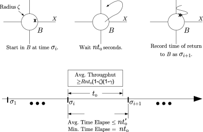
Figure 4: The top half of the figure illustrates the definition of the stopping times $\sigma_{i},\sigma_{i+1},\ldots\,$. The bottom half illustrates the intuition behind the proof of Theorem 4 by plotting the stopping times on a time line, and showing the bound on expected throughput between such stopping times.

the $\zeta$-neighborhood of $h\mathcal{E}$ that occurs at least $nt_{0}$ seconds after the last stopping time. We define random vectors $\rho_{i}$ that track the cumulative service, divided by average service times, between stopping times and relate these to the desired rate vector $R$ using Theorem 2. We use ergodicity to argue that the long-term average rates exist, and that this long-term limit must equal the product of the expected value of $\rho_{i}$ times the lim inf of $t/N(t)$ the inverse of the arrival rate of stopping times. Due to Lemma 2, this later quantity has an upper bound of $nt_{0}$ times a constant that can be made small.

Theorem 4

Suppose for some $t_{0}>0$ and some closed, bounded $\mathcal{E}\in\bar{\mathsf{X}}$ both of the following are true:

• For any fluid model trajectory $\bar{\mathfrak{X}}(\cdot)$ and $\bar{h}\geq 0$ that satisfies (12)–(24),

  $$\bigl{\|}\bar{X}(t)\bigr{\|}_{\bar{h}\mathcal{E}}\equiv 0\qquad\forall t\geq t_{0}\bigl{\|}\bar{X}(0)\bigr{\|}_{\bar{h}\mathcal{E}}.$$ (35)

• For any fluid model trajectory $\bar{\mathfrak{X}}(\cdot)$ and $\bar{h}>0$ that satisfies (12)–(24),

  $$M^{-1}\dot{\bar{T}}(t)\equiv R\qquad\forall t\geq t_{0}\bigl{\|}\bar{X}(0)\bigr{\|}_{\bar{h}\mathcal{E}},$$ (36)

  where $R\in\mathbb{R}^{K}_{+}$.

Then for any $\epsilon>0$, there exists a $n_{c}>0$ such that for all $n\geq n_{c}$,

$$\lim_{t\rightarrow\infty}\frac{D^{\mathbf{x}}(t)}{t}\geq(1-\epsilon)R\qquad\mbox{a.s.}$$

We observe that equations (36) and (35) are the necessary conditions to apply Theorems 2 and 3, respectively. Therefore, we may arbitrarily pick the constants $\zeta$, $\delta$ and $b$ of Theorem 3 and the constants $\zeta$ and $\gamma$ of Theorem 2 (using the same $\zeta$ value in Theorems 2 as we use when we apply Theorem 3), and then fix an $n$ satisfying

$$n>\max\bigl{[}L_{1}(\zeta,\gamma),\zeta^{-1}L_{2}(\zeta,\delta),L_{3}(\zeta,b)\bigr{]}$$ (37)

so that the conclusions of both Theorems 3 and 2 hold.

In addition, conclusions (i) and (ii) of Theorem 3 allow us to invoke Lemma 2 to complete (33) where $\tau_{B}^{n}(nt_{0})$ is defined by (34). Because the constants $\zeta$, $b$, $\delta$ can be chosen arbitrarily, equations (33) and (37) imply that the ratio of the expected first hitting time of $B$ ($nt_{0}$ seconds after having started in $B$) to $nt_{0}$ can be made to be close to $1$ by choosing $n$ large enough. We collect some of the constants in (33) in the term $t_{0}^{\prime}$ defined by

$$nt_{0}^{\prime}=nt_{0}\biggl{[}1+\frac{\zeta+b}{1-\delta}\biggr{]}.$$ (38)

We have also chosen $n$ large enough so that the following conclusion from Theorem 2 holds:

$$\inf_{\|x/n\|_{h\mathcal{E}}\leq\zeta}\mathrm{E}\bigl{[}T^{\mathbf{x}}(nt_{0})\bigr{]}\geq MR(1-\zeta)(1-\gamma)nt_{0}.$$ (39)

Define the stopping times

$$\sigma_{0}=0,\qquad\sigma_{i+1}=\inf\bigl{\{}t\geq nt_{0}+\sigma_{i}\dvtx X(t)\in B\bigr{\}}\qquad\forall i\geq 0.$$ (40)

Figure 4 illustrates how these stopping times are defined. Note that for any initial condition $x\in\mathrm{X}$ (the state space of $X^{n}$) and index $i\geq 1$,

$$\mathrm{E}_{x}[\sigma_{i+1}-\sigma_{i}]\leq\sup_{\tilde{x}\in B}\mathrm{E}_{\tilde{x}}\bigl{[}\tau_{B}^{n}(nt_{0})\bigr{]}\leq nt_{0}^{\prime}.$$ (41)

This follows from the fact that $X^{\mathbf{x}}(\sigma_{i})\in B$, the strong Markov property, the stopping time definitions (34) and (40) and expressions (33) and (38). Also, $X$ is positive Harris recurrent by Lemma 2 and therefore, $\mathrm{E}_{x}[\sigma_{1}]<\infty$ for any $x\in\mathrm{X}$. We define a counting process $N(t)$ for the stopping times $\sigma_{i}$ as $N(t)=\inf\{i\dvtx\sigma_{i}\leq t\}.$ Because $X$ is positive Harris recurrent, $\sigma_{i}<\infty$ almost surely, and therefore $N(t)\rightarrow\infty$ a.s. We now turn to bounding the expected “arrival” rate of the stopping times $\sigma_{i}$. By (41) for each $i$,

$$\frac{\mathrm{E}_{x}[\sigma_{i}]}{i}=\frac{\sum_{j=1}^{i-1}\mathrm{E}_{x}[\sigma_{j+1}-\sigma_{j}]+\mathrm{E}_{x}\sigma_{1}}{i}\leq nt_{0}^{\prime}(1-1/i)+\frac{\mathrm{E}_{x}\sigma_{1}}{i}.$$ (42)

Additionally, along any sample path

$$\frac{t}{N(t)}\leq\frac{\sigma_{N(t)+1}}{N(t)+1}\frac{N(t)+1}{N(t)}.$$

Thus by taking $\liminf_{t\rightarrow\infty}E_{x}(\cdot)$ of both sides, and using (42) we have

$$\liminf_{t\rightarrow\infty}\mathrm{E}_{x}\biggl{[}\frac{t}{N(t)}\biggr{]}\leq nt_{0}^{\prime}.$$

Moreover, by Fatou’s lemma

$$\mathrm{E}_{x}\biggl{[}\liminf_{t\rightarrow\infty}\frac{t}{N(t)}\biggr{]}\leq\liminf_{t\rightarrow\infty}\mathrm{E}_{x}\biggl{[}\frac{t}{N(t)}\biggr{]}\leq nt_{0}^{\prime}.$$ (43)

We define the random vectors $\rho_{i}=M^{-1}[{T}^{n}(\sigma_{i}+\sigma_{i+1})-{T}^{n}(\sigma_{i})]$ to track the service between stopping times $\sigma_{i}$. Note that for $i\geq 1$ and each $x\in\mathrm{X}$,

$$\mathrm{E}_{x}[\rho_{i}]\geq\inf_{\tilde{x}\in B}\mathrm{E}_{\tilde{x}}\bigl{[}M^{-1}{T}^{\tilde{x},n}(nt_{0})\bigr{]}\geq Rnt_{0}(1-\zeta)(1-\gamma).$$ (44)

This follows from the fact that $X^{\mathbf{x}}(\sigma_{i})\in B$, the strong Markov property, the definition of $\sigma_{i}$ (40), the definition of $\rho_{i}$, and relation (39). Figure 4 illustrates the fact that the throughput between stopping times $\sigma_{i}$ and $\sigma_{i+1}$ is lower-bounded according to relation (44).

By DaiMeyn the following ergodic property holds for every measurable $f$ on $\mathrm{X}$ with $\pi(|f|)<\infty$,

$$\lim_{t\rightarrow\infty}\frac{1}{t}\int_{0}^{t}f\bigl{(}X^{n}(s)\bigr{)}\,ds=\pi(f)\qquad\mbox{$\mathrm{P}_{x}$-a.s. for each $x\in\mathrm{X}$},$$

where $\pi$ is the unique invariant distribution of $X^{n}$. Assigning the function $f(x)\triangleq M^{-1}\dot{T}^{\mathbf{x}}(0)$ to be the instantaneous service rates when the process is in state $x$ (recall that we assumed the service rates are a function of the state in Section 2), we have

$$\lim_{t\rightarrow\infty}\frac{1}{t}\int_{0}^{t}f\bigl{(}X^{\mathbf{x}}(s)\bigr{)}\,ds=\lim_{t\rightarrow\infty}\frac{1}{t}M^{-1}\widetilde{T}{}^{\mathbf{x}}(t)=\mathcal{R}\qquad\mbox{a.s.}$$ (45)

for some constant vector $\mathcal{R}$.

Consider the random variable $\mathcal{N}\triangleq\liminf_{t\rightarrow\infty}\frac{t}{N(t)}.$ The random variable $\mathcal{N}$ is a $\mathrm{P}_{\pi}$ invariant random variable, and therefore is a constant. Moreover by (43), $\mathcal{N}\leq nt_{0}^{\prime}$. A more detailed explanation of this argument is provided in MusacchioPhD .

We observe that for any sample path the following inequalities hold:

$$\frac{t}{N(t)}\frac{M^{-1}{T}^{\mathbf{x}}(t)}{t}\leq\frac{\sum_{j=0}^{N(t)}\rho_{j}}{N(t)}\leq\frac{t}{N(t)}\frac{\sigma_{N(t)+1}}{t}\frac{M^{-1}{T}^{\mathbf{x}}(\sigma_{N(t)+1})}{\sigma_{N(t)+1}}.$$ (46)

Taking the $\liminf_{t\rightarrow\infty}$ of both sides and using (45), we have that

$$\liminf_{t\rightarrow\infty}\frac{\sum_{j=0}^{N(t)}\rho_{j}}{N(t)}=\mathcal{N}\mathcal{R}\qquad\mbox{a.s.}$$ (47)

We note that ${{T}^{\mathbf{x}}(\sigma_{N(t)+1})}/{\sigma_{N(t)+1}}\leq\mathbf{1}$ where $\mathbf{1}$ is a column vector of 1’s of appropriate dimension. This fact combined with (46) yields that for each $i>0$,

$$\inf_{k\geq i}\frac{\sum_{j=1}^{k}{\rho}_{j}}{i}\leq\liminf_{t\rightarrow\infty}\frac{t}{N(t)}M^{-1}\mathbf{1}\leq nt_{0}^{\prime}M^{-1}\mathbf{1}.$$

Thus the random variables $\{\inf_{k\geq i}i^{-1}\sum_{j=1}^{k}{\rho}_{j}\dvtx i>0\}$ are dominated by a constant. Consequently, $\liminf_{i\rightarrow\infty}\mathrm{E}[{\sum_{j=1}^{i}{\rho}_{j}}/{i}]=\mathcal{N}\mathcal{R}$ by the dominated convergence theorem. Also for each $i>0$, $\mathrm{E}[{\sum_{j=1}^{i}{\rho}_{j}}/{i}]\geq Rnt_{0}(1-\gamma)(1-\zeta)$ by (44). Thus, $\mathcal{N}\mathcal{R}\geq Rnt_{0}(1-\gamma)(1-\zeta).$ Substituting (43) we have that $\mathcal{R}\geq(1-\gamma)(1-\zeta)\frac{t_{0}}{t_{0}^{\prime}}R.$ This implies

$$\lim_{t\rightarrow\infty}\frac{1}{t}M^{-1}T^{\mathbf{x}}(t)\geq\frac{(1-\gamma)(1-\zeta)}{1+({\zeta+b})/({1-\delta})}R\qquad\mbox{a.s.}$$

Recall $\gamma$, $\zeta$, $b$ and $\delta$ may be chosen arbitrarily small, so long as $n$ is chosen large enough according to (37). Thus, for any $\epsilon>0$ there exisits an $n$ such that

$$\lim_{t\rightarrow\infty}\frac{1}{t}M^{-1}T^{\mathbf{x}}(t)\geq(1-\epsilon)R\qquad\mbox{a.s.}$$

By the strong law of large numbers for renewal processes Durrett , $\frac{1}{t}S_{k}^{\mathbf{x}}(t)\rightarrow m_{k}$ a.s. Thus by (9), $\lim_{t\rightarrow\infty}\frac{1}{t}D^{\mathbf{x}}(t)\geq(1-\epsilon)R$ a.s.

4 Analysis of switch example

In this section we apply the results of the preceding section to the example introduced in Section 1.3. Recall that this example resembles a 2-input 2-output switch and has 3 flows and is illustrated by Figure 3. As we discussed in Section 1.3, the max-min fair share rate allocation would be that all three flows achieve rates of $0.5$, so we set $R=[0.5,0.5,0.5]^{T}$ to be the vector of desired rates.

To fit the framework we have developed, we must show that the fluid model with thresholds $\bar{h}$ is drawn to a set $\bar{h}\mathcal{E}$, and that the fluid model rates while in $\bar{h}\mathcal{E}$ are $R$. Intuition suggests that the dynamics of the fluid model should evolve in the following way:

• One of the queues flow 2 passes through (either queue 2 or 7) reaches threshold and “chatters” there. The other queue can be anywhere at or below its threshold. By “chatters” we mean that it alternately goes a tiny amount above and below. However, if the differential inclusions of the fluid model are such that: (i) the queue grows whenever below threshold or (ii) shrinks when above, then a fluid model trajectory would go to threshold and stay there.

• Queue 1 fills to threshold, “chatters” there, limiting flow 1’s ultimate rate.

• Queue 7 fills to threshold, “chatters” there, limiting flow 3’s ultimate rate.

• Other queues are not “bottlenecks” and should empty.

This above intuition suggests that the fluid model is drawn to the set $\bar{h}\tilde{\mathcal{E}}$ where $\tilde{\mathcal{E}}$ is given by

$$\tilde{\mathcal{E}} \triangleq \bigl{\{}\bar{X}\dvtx\bar{Q}_{1}=\bar{Q}_{8}=1,\bar{Q}_{3}=\bar{Q}_{4}=\bar{Q}_{5}=\bar{Q}_{6}=0,$$

$$\hskip 4.0pt(\bar{Q}_{2},\bar{Q}_{7})\in\bigl{\{}[0,1]\times 1\bigr{\}}\cup\bigl{\{}1\times[0,1]\bigr{\}},\bar{U}=0,\bar{V}=0,\bar{H}=0\bigr{\}}.$$

As it will turn out, the most critical part of the analysis of this example’s fluid model is to show that the queues flow 2 passes through, queues 2 and 7, go to values in $\bar{h}\tilde{\mathcal{E}}$ in a time not more than a constant times their initial values. Intuition suggests that after a “settling down” period flow 1’s rate through queue 1, as well as flow 3’s rate through queue 8, settles to $0.5$. After flow 1 and flow 3’s rates settle, the dynamics of

Table 1: Dynamics of $(\bar{Q}_{2}(t),\bar{Q}_{7}(t))$, after flows 1 and 3 settle to their ultimate rates of 0.5. The rows numbers correspond to the regions labeled in the phase portrait diagram of Figure 5

	$\bolds{\bar{Q}_{2}}$	$\bolds{\bar{Q}_{7}}$	$\bolds{\dot{\bar{Q}}_{2}}$	$\bolds{\dot{\bar{Q}}_{7}}$	Time to $\bolds{\bar{h}\mathcal{E}}$	$\bolds{\frac{\mathrm{Time}\ \mathrm{to}\ \bar{h}\mathcal{E}}{\|\bar{X}\|_{\bar{h}\mathcal{E}}}}$
1	$[0,\bar{h})$	$[0,\bar{h})$	$-$0.1	0	if $|\bar{Q}_{7}-\bar{h}|<a\bar{h}$ then	$\frac{10}{a}$
					$\frac{10}{a}|\bar{Q}_{7}-\bar{h}|$
					if $|\bar{Q}_{7}-\bar{h}|\geq a\bar{h}$ then
					$10|\bar{Q}_{2}-\bar{h}|$
2	$(\bar{h},\infty)$	$[0,\bar{h})$	$-$0.5	0	$2|\bar{Q}_{2}-\bar{h}|$	2
3	$(0,\infty)$	$(\bar{h},\infty)$	$-$0.5	0	if $|\bar{Q}_{7}-\bar{h}|<a\bar{h}$ then	$\frac{2}{a}$
					$\frac{2}{a}|\bar{Q}_{7}-\bar{h}|$
					if $|\bar{Q}_{7}-\bar{h}|\geq a\bar{h}$ then
					$2|\bar{Q}_{2}-\bar{h}|+2|\bar{Q}_{7}-\bar{h}-a\bar{h}|$
4	0	$(\bar{h},\infty)$	0	$-$0.5	$2|\bar{Q}_{7}-\bar{h}-a|$	2
5	$\bar{h}$	$[0,\bar{h}]$	$[-0.5,0.1]$	$[-0.5,0]$	0	N$/$A
6	$[0,\bar{h}]$	$\bar{h}$	$[-0.5,0.1]$	$[-0.5,0]$	0	N$/$A

$(\bar{Q}_{2}(t),\bar{Q}_{7}(t))$, the queues of flow 2, follow the relations outlined by Table 1 and illustrated by Figure 5. The entries of Table 1 are easily derived by using the observations that:

• The arrival rate to queue 2 is 0.6 when queue 2 and queue 7 are below threshold while the arrival rate to queue 2 is 0 when one of these queues is above threshold.

• The departure rate from either queue 2 or queue 7 is 0.5 whenever the queue is nonempty or has sufficient arrivals to maintain this departure rate. (This relies on our assumption that the flow rates through queues 1 and 8 have “settled down” to $0.5$.)

Figure 5 is a vector flow diagram, showing the dependence of $(\dot{\bar{Q}}_{2}(\cdot),\dot{\bar{Q}}_{7}(\cdot))$ on $(\bar{Q}_{2}(\cdot),\bar{Q}_{7}(\cdot))$. It is evident from the diagram that the time to reach the set

$$\bigl{\{}[0,\bar{h}]\times\bar{h}\bigr{\}}\cup\bigl{\{}\bar{h}\times[0,\bar{h}]\bigr{\}},$$

which is the projection of $\bar{h}\tilde{\mathcal{E}}$ on to the subspace on which $(\bar{Q}_{2}(\cdot),\bar{Q}_{7}(\cdot))$ takes values, is not always less than or equal to a constant times the initial condition’s distance from this set. Consider an initial condition of $(\frac{\bar{h}}{2},\bar{h}+\epsilon)$. This initial condition is only a distance of $\epsilon$ from $\tilde{\mathcal{E}}$, but the time it takes to reach the set $\tilde{\mathcal{E}}$ is $\bar{h}+\frac{1}{2}\epsilon$. (Note

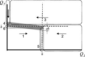
Figure 5: The evolution of $(\bar{Q}_{2}(t),\bar{Q}_{7}(t))$. The shaded area indicates the set $\bar{h}\mathcal{E}$.

that we will use the $L^{1}$ norm throughout this section.) This is the same phenomenon we observed in the example in the Introduction of the paper. There, as here, we can fix the problem by slightly enlarging the set $\tilde{\mathcal{E}}$ to a new set $\mathcal{E}$ so that the set is reached in a time not more than a constant times the initial condition’s starting distance from the set. To this end, we define $\mathcal{E}$ according to

$$\mathcal{E} \triangleq \bigl{\{}\bar{X}\dvtx\bar{Q}_{1}=\bar{Q}_{8}=1,\bar{Q}_{3}=\bar{Q}_{4}=\bar{Q}_{5}=\bar{Q}_{6}=0,$$

$$\hskip 4.7pt(\bar{Q}_{2},\bar{Q}_{7})\in\bigl{\{}(\chi,\psi)\dvtx\chi\in[0,1],\psi\in\bigl{[}1-a\chi,1+a(1-\chi)\bigr{]}\bigr{\}}$$

$$\hskip 112.3pt{}\cup\bigl{\{}1\times[0,1]\bigr{\}},\bar{U}=0,\bar{V}=0,\bar{H}=0\bigr{\}}.$$

Here $a$ is an arbitrary positive constant that should be less than $1$. The projection of this set onto the subspace spanned by $(Q_{2},Q_{7})$ is shown as the shaded area in Figure 5. With this definition, one can show that the set $\bar{h}\mathcal{E}$ is reached in a time not more than a constant times the initial distance from $\bar{h}\mathcal{E}$. The time to reach $\bar{h}\mathcal{E}$, along with the maximum ratio of the time to reach $\bar{h}\mathcal{E}$ divided by initial distance to $\bar{h}\mathcal{E}$ are shown in Table 1.

We are now ready to formalize the intuition we have outlined in the preceding paragraphs. We begin by stating a lemma that the system settles down so that the behavior flow 2’s queues are as described by Table 1 after a time $\tau_{sd}$ (mnemonic for “settle down”) that is in proportion to the initial condition.

Lemma 3

There exists a time $\tau_{sd}$ proportional to the initial condition as described by the relation

$$\tau_{sd}=t_{01}\bigl{\|}\bar{X}(0)\bigr{\|}_{\bar{h}\mathcal{E}}$$

for some positive $t_{01}$ such that for all regular points $t\geq\tau_{sd}$:

• The value of $(\dot{\bar{Q}}_{2}(t),\dot{\bar{Q}}_{7}(t))$ is determined by the value of $(\bar{Q}_{2}(t),\bar{Q}_{7}(t))$ as specified by Table 1.

• $\bar{Q}_{3}(t)=\bar{Q}_{5}(t)=\bar{Q}_{6}(t)=0$, and $\bar{Q}_{8}(t)=\bar{h}$.

• The time to reach the set $\bar{h}\mathcal{E}$, as well as the maximum ratio between this time and the distance of $(\bar{Q}_{2}(\tau_{sd}),\bar{Q}_{7}(\tau_{sd}))$ from $\bar{h}\mathcal{E}|_{\bar{Q}_{2},\bar{Q}_{7}}$ in any of the regions 1 through 4 is as specified in Table 1. [Here $\bar{h}\mathcal{E}|_{\bar{Q}_{2},\bar{Q}_{7}}$ denotes the projection of the set $\bar{h}\mathcal{E}$ onto the space on which $(\bar{Q}_{2},\bar{Q}_{7})$ takes values.]

Lemma 3 is proved by using relations (12)–(24) that describe the evolution of a fluid model trajectory. The proof is straightforward but slightly lengthy because it requires analysis for each entry in Table 1. We therefore omit this proof.

We now state and prove the principal result of this section.

Theorem 5

For any $\epsilon>0$, there exists an $n_{c}>0$ such that if the discarding thresholds of the stochastic system in Example 2 are set to $nh$, $n\geq n_{c}$, then

$$\lim_{t\rightarrow\infty}\frac{D(t)}{t}\geq(1-\epsilon)\frac{1}{2}\mathbf{1}\qquad\mbox{a.s.},$$

where $\mathbf{1}$ is a vector of ones of dimension $K$.

By Lemma 3 the dynamics of the state variables $(\bar{Q}_{2}(t),\bar{Q}_{7}(t))$ of the fluid model trajectory evolve according to Table 1 after a time $\tau_{sd}=t_{01}\|\bar{X}(0)\|_{\bar{h}\mathcal{E}}$. From Table 1, the $\bar{Q}_{2}$ and $\bar{Q}_{7}$ components of the fluid model trajectory reach values in the set $\bar{h}\mathcal{E}$’s projection in, at most, an additional $\frac{10}{a}\|\bar{X}(\tau_{sd})\|_{\bar{h}\mathcal{E}}$ time units. Because the total arrival rate into the system is less than or equal to $1.8$,

$$\bigl{\|}\bar{X}(\tau_{sd})\bigr{\|}_{\bar{h}\mathcal{E}}\leq(2t_{01}+1)\bigl{\|}\bar{X}(0)\bigr{\|}_{\bar{h}\mathcal{E}}.$$

Thus after a time $t_{02}\|\bar{X}(0)\|_{\bar{h}\mathcal{E}}$, where $t_{02}=\frac{10}{a}(2t_{01}+1)+1,$ all queues but queue 1 have been shown to reach values in the projection of the set $\bar{h}\mathcal{E}$. By Lemma 3, queue 5 is empty, so either: queue 1 is above threshold, in which case discarding is on and it will reach threshold in $2(\bar{Q}_{1}(t_{02}\|\bar{X}(0)\|_{\bar{h}\mathcal{E}})-\bar{h})$ time units, or queue 1 is below threshold in which case it will reach threshold in $10(\bar{Q}_{1}(t_{02}\|\bar{X}(0)\|_{\bar{h}\mathcal{E}})-\bar{h})$ time units. Once $\bar{Q}_{1}(t)$ reaches threshold $\bar{h}$, it remains there by the following reasoning. If queue 1 were to move some positive amount $\epsilon$ above $\bar{h}$, the discarding would have turned on before the queue grew to $\epsilon$ and prevented it from getting there. Similarly, if queue 1 were to move some positive amount $\epsilon$ below $\bar{h}$, the discarding would have turned off before the queue receded by $\epsilon$, and prevented the queue from receding that much. Very loosely, we can bound the rate of growth of queue 1 before time $t_{02}\|\bar{X}(0)\|_{\bar{h}\mathcal{E}}$ by

$$\bar{Q}_{1}\bigl{(}t_{02}\bigl{\|}\bar{X}(0)\bigr{\|}_{\bar{h}\mathcal{E}}\bigr{)}\leq 1.6\bigl{\|}\bar{X}(0)\bigr{\|}_{\bar{h}}.$$

Thus after a time of length $t_{0}\|\bar{X}(0)\|_{\bar{h}\mathcal{E}}$, where $t_{0}$ is given by $t_{0}=\frac{10}{a}(2t_{01}+1)+17$, all fluid model trajectories will have reached the set $\bar{h}\mathcal{E}$. The departure rates for all three flows, as well as the departure rates for each class associated with each flow, are easily seen to be $0.5$ when the fluid model’s state is in $\bar{h}\mathcal{E}$ and threshold $\bar{h}>0$. Thus, by Theorem 4 we have that the asymptotic flow rates approach $0.5$.

5 Conclusion

In this work we have shown how the analysis of the flow rates of a stochastic network with a particular flow control scheme may be reduced to an analysis of a fluid model. While we have focused on a particular flow control scheme, the same analysis could be carried out for many other control schemes. The key feature that enabled our approach was that our control scheme has a free parameter, $n$, which when increased makes the system look more and more like a deterministic fluid system. We have demonstrated how to use the theory developed in this paper to analyze an example network resembling a 2-input, 2-output switch.

Appendix

Before proving Theorem 1, we state and prove a number of lemmas. Lemma 4 is a functional form of the strong law of large numbers for renewal processes, and is taken from Dai95 . Lemma 5 is a new result showing that the thinned arrivals (the customers that make it beyond the discarding point) converge to a fluid limit along a subsequence. Lemma 6 is a result taken from Dai95 showing that the residual initial arrival and service times decline to zero at rate $1$ in the fluid limit. The lemma also shows that the sequence of functions we use to take the fluid limit are uniformly integrable.

Also the lemmas will make use of fluid limits that have well-defined limiting residual interarrival and service times, as defined by the following property.

Property 2.

$\{({{\mathbf{x}}_{j}},a_{j})\}$ is a sequence for which $\frac{U^{{\mathbf{x}}_{j}}(0)}{a_{j}}\rightarrow\bar{U}(0)$, $\frac{V^{{\mathbf{x}}_{j}}(0)}{a_{j}}\rightarrow\bar{V}(0)$, for some $\bar{U}(0)\geq 0$ and $\bar{V}(0)\geq 0$.

Lemma 4 ((Dai, Lemma 4.2 of Dai95 ))

Suppose that $\{({{\mathbf{x}}_{j}},a_{j})\}$ is a sequence satisfying Properties 1 and 2 (see pages 1 and 2). Then for almost all $\omega$,

$$\frac{E_{f}^{\mathbf{x}_{j}}(a_{j}t)}{a_{j}} \rightarrow \alpha_{f}\bigl{(}t-\bar{U}_{f}(0)\bigr{)}^{+}\qquad\mbox{u.o.c.},$$

$$\frac{S_{k}^{\mathbf{x}_{j}}(a_{j}t)}{a_{j}} \rightarrow \mu_{k}\bigl{(}t-\bar{V}_{k}(0)\bigr{)}^{+}\qquad\mbox{u.o.c.}$$

See Lemma 4.2 of Dai Dai95 . The result is an instance of the strong law of large numbers for renewal processes Durrett .

Lemma 5 ((Thinned arrival convergence))

Suppose that $\{({{\mathbf{x}}_{j}},a_{j})\}$ is a sequence satisfying Properties 1 and 2. Then for almost all $\omega$, there exists a subsequence $\{({{\mathbf{x}}_{m}},a_{m})\}\subseteq\{({{\mathbf{x}}_{j}},a_{j})\}$ such that

$${\Lambda^{\mathbf{x}_{m}}(a_{m}t)}/{a_{m}}\rightarrow\bar{\Lambda}(t)\qquad\mbox{u.o.c.},$$

where $\bar{\Lambda}(t)$ is some Lipschitz continuous process with, for all regular $t\geq 0$,

$$\dot{\bar{\Lambda}}_{f}(t)\leq\alpha_{f}\qquad\mbox{for each flow $f$.}$$ (48)

By Lemma 4,

$${E_{f}^{\mathbf{x}_{j}}(a_{j}t)}/{a_{j}}\rightarrow\alpha_{f}\bigl{(}t-\bar{U}_{f}(0)\bigr{)}^{+}\qquad\mbox{u.o.c.}$$ (49)

for each flow $f$. For notational convenience in the development that follows, we define

$$\bar{E}_{f}(t)\triangleq\alpha_{f}\bigl{(}t-\bar{U}_{f}(0)\bigr{)}^{+},\qquad\Delta_{j}(t)\triangleq{E^{\mathbf{x}_{j}}(a_{j}t)}/{a_{j}}-\bar{E}(t).$$ (50)

Pick a compact time interval $[s_{0},s_{1}]$. Since the number of admitted customers is not greater than the number that arrive,

$$\frac{1}{a_{j}}\bigl{[}\Lambda^{\mathbf{x}_{j}}\bigl{(}a_{j}(t+\varepsilon)\bigr{)}-\Lambda^{\mathbf{x}_{j}}(a_{j}t)\bigr{]}\leq\frac{1}{a_{j}}\bigl{[}E^{\mathbf{x}_{j}}\bigl{(}a_{j}(t+\varepsilon)\bigr{)}-E^{\mathbf{x}_{j}}(a_{j}t)\bigr{]}$$ (51)

for any positive $\varepsilon\leq s_{1}-s_{0}$ and $t\dvtx s_{0}\leq t\leq s_{1}-\varepsilon$. Adding $-\Delta_{j}(t+\varepsilon)$ and $\Delta_{j}(t)$ to both sides and substituting (50), we have

$$\frac{\Lambda^{\mathbf{x}_{j}}(a_{j}(t+\varepsilon))}{a_{j}}-\Delta_{j}(t+\varepsilon)-\biggl{[}\frac{\Lambda^{\mathbf{x}_{j}}(a_{j}t)}{a_{j}}-\Delta_{j}(t)\biggr{]}\leq\bar{E}(t+\varepsilon)-\bar{E}(t)\leq\varepsilon\alpha.$$

Define the family of functions

$$\mathfrak{L}_{j}(s_{0},t):=\sup_{s\in[s_{0},t]}\biggl{[}\frac{\Lambda^{\mathbf{x}_{j}}(a_{j}s)}{a_{j}}-\Delta_{j}(s)\biggr{]}$$

for $t\in[s_{0},s_{1}]$. Because the argument of the $\sup$ function is a vector, $\sup$ is taken component-wise. Note that for any $(t,\varepsilon)$ with $t\in[s_{0},s_{1}-\varepsilon]$,

$$\mathfrak{L}_{j}(s_{0},t+\varepsilon)=\mathfrak{L}_{j}(s_{0},t)\vee\mathfrak{L}_{j}(t,t+\varepsilon)$$

and

$$\mathfrak{L}_{j}(t,t+\varepsilon)\leq\varepsilon\alpha+\mathfrak{L}_{j}(t,t)\leq\varepsilon\alpha+\mathfrak{L}_{j}(s_{0},t).$$

Thus $\mathfrak{L}_{j}(s_{0},t+\varepsilon)-\mathfrak{L}_{j}(s_{0},t)\leq\varepsilon\alpha$ and clearly $\mathfrak{L}_{j}(s_{0},t+\varepsilon)-\mathfrak{L}_{j}(s_{0},t)\geq 0$ because $\mathfrak{L}_{j}(s_{0},\cdot)$ is monotone. Hence the functions $\mathfrak{L}_{j}(s_{0},\cdot)$ are equicontinuous and individually Lipschitz continuous. Thus, by Arzela’s theorem, there exists a further subsequence $\{({{\mathbf{x}}_{m}},a_{m})\}\subseteq\{({{\mathbf{x}}_{j}},a_{j})\}$ such that

$$\mathfrak{L}_{m}(s_{0},t)\rightarrow\bar{\Lambda}(t)$$

uniformly on the compact set $t\in[s_{0},s_{1}]$ for some monotone-nondecreasing, Lipschitz-continuous process $\bar{\Lambda}(t)$. But by (49), $\Delta_{j}(t)\rightarrow 0$ uniformly on compact sets. Because of this and the fact that $\Lambda^{\mathbf{x}_{j}}(a_{j}s)/a_{j}$ is monotone in $s$, it follows that $\mathfrak{L}_{j}(s_{0},t)$ approaches $\Lambda^{\mathbf{x}_{j}}(a_{j}t)/a_{j}$ as $j\rightarrow\infty$. Thus

$$\sup_{s\in[s_{0},t]}\biggl{[}\frac{\Lambda^{\mathbf{x}_{j}}(a_{j}s)}{a_{j}}-\Delta_{j}(s)\biggr{]}\rightarrow\frac{\Lambda^{\mathbf{x}_{j}}(a_{j}t)}{a_{j}}\rightarrow\bar{\Lambda}(t).$$

Because the choice of $[s_{0},s_{1}]$ was arbitrary, we have $\Lambda^{\mathbf{x}_{m}}(a_{m}s)/a_{m}\rightarrow\bar{\Lambda}(t)$ u.o.c. Furthermore, (49) and (51) imply that $\bar{\Lambda}(t)$ satisfies (48).

Lemma 6 ((Lemmas 4.3 and 4.5 of Dai Dai95 ))

Suppose that $\{({{\mathbf{x}}_{j}},a_{j})\}$ is a sequence satisfying Properties 1 and 2. Then almost surely

$$\lim_{j\rightarrow\infty}\frac{U_{f}^{\mathbf{x}_{j}}(a_{j}t)}{a_{j}} = \bigl{(}\bar{U}_{f}(0)-t\bigr{)}^{+}\qquad\mbox{u.o.c.},$$

$$\lim_{j\rightarrow\infty}\frac{V_{k}^{\mathbf{x}_{j}}(a_{j}t)}{a_{j}} = \bigl{(}\bar{V}_{k}(0)-t\bigr{)}^{+}\qquad\mbox{u.o.c.}$$

Also, for each fixed $t\geq 0$, the sets of functions

$$\displaystyle\bigl{\{}U^{{\mathbf{x}}_{j}}(a_{j}t)/a_{j}\dvtx a_{j}\geq 1\bigr{\}},\qquad\bigl{\{}V^{{\mathbf{x}}_{j}}(a_{j}t)/a_{j}\dvtx a_{j}\geq 1\bigr{\}},$$

$$\displaystyle\bigl{\{}Q^{{\mathbf{x}}_{j}}(a_{j}t)/a_{j}\dvtx a_{j}\geq 1\bigr{\}}$$

are uniformly integrable.

See Lemmas 4.3 and 4.5 of Dai Dai95 .

We use the following lemma later to show that because all of the systems we consider are work-conserving, the fluid limit must also be work-conserving. In the lemma below, the notation $D_{\mathbb{R}}[0,\infty)$ denotes the space of right-continuous functions on $\mathbb{R}_{+}$ having left limits on $(0,\infty)$, and endowed with the Skorohod topology EthierKurtz . $C_{\mathbb{R}}[0,\infty)\subset D_{\mathbb{R}}[0,\infty)$ is the subset of continuous paths.

Lemma 7 ((Lemma 2.4 of Dai and Williams DaiWilliams ))

Let $\{(z_{j},\chi_{j})\}$ be a sequence in $D_{\mathbb{R}}[0,\infty)\times C_{\mathbb{R}}[0,\infty)$. Assume that $\chi_{j}$ is nondecreasing and $(z_{j},\chi_{j})$ converges to $(z,\chi)\in C_{\mathbb{R}}[0,\infty)\times C_{\mathbb{R}}[0,\infty)$ u.o.c. Then for any bounded continuous function $f$,

$$\int_{0}^{t}f\bigl{(}z_{j}(s)\bigr{)}\,d\chi_{j}(s)\rightarrow\int_{0}^{t}f\bigl{(}z(s)\bigr{)}\,d\chi(s)\qquad\mbox{u.o.c.}$$

See Lemma 2.4 of Dai and Williams DaiWilliams .

We are now ready to prove Theorem 1.

Proof of Theorem 1 Before scaling space, the discarding thresholds for each $j$ are $n_{j}h$. After scaling space by $a_{j}$, the scaled thresholds are $n_{j}h/a_{j}$. Property 1 insures that $n_{j}/a_{j}$ is upper bounded by a constant. Thus by the Bolzano–Weierstrass theorem, there exists a subsequence $\{({{\mathbf{x}}_{r}},a_{r})\}\subseteq\{({{\mathbf{x}}_{j}},a_{j})\}$ for which $n_{r}h/a_{r}\rightarrow\bar{h}$ for some $\bar{h}\geq 0$.

Property 1 insures that $\|x_{r}/a_{r}\|_{{n_{r}h}/{a_{r}}\mathcal{E}}$ is upper bounded by a constant. Thus $\limsup\|x_{r}/a_{r}\|_{\bar{h}\mathcal{E}}$ is finite. Consequently, there must be some further subsequence $\{({{\mathbf{x}}_{u}},a_{u})\}\subseteq\{({{\mathbf{x}}_{r}},a_{r})\}$ for which ${x_{u}}/{a_{u}}\rightarrow\bar{X}(0)$ for some finite $\bar{X}(0)$.

The hysteresis variables satisfy $H^{\mathbf{x}_{u}}(a_{u}t)/a_{u}\rightarrow 0$ u.o.c. because $H^{\mathbf{x}_{u}}(a_{u}t)$ is bounded by a constant by its definition. This fact along with the convergence of $X^{{\mathbf{x}}_{u}}(0)/a_{u}\rightarrow\bar{X}(0)$ allows us to use Lemma 6 to conclude $U^{\mathbf{x}_{u}}(a_{u}t)/\break a_{u}\rightarrow\bar{U}(t)$ and $V^{\mathbf{x}_{u}}(a_{u}t)/a_{u}\rightarrow\bar{V}(t)$ u.o.c. where $\bar{U}(t)$ and $\bar{V}(t)$ satisfy (12).

The cumulative service time process $T^{\mathbf{x}_{u}}$ satisfies

$$\bigl{[}T^{\mathbf{x}_{u}}(a_{u}t)-T^{\mathbf{x}_{u}}(a_{u}s)\bigr{]}/a_{u}\leq(t-s).$$ (52)

Thus by Arzela’s theorem munkres , there exists a further subsequence $\{({{\mathbf{x}}_{v}},a_{v})\}\subseteq\{({{\mathbf{x}}_{u}},a_{u})\}$ for which ${T^{\mathbf{x}_{v}}(a_{v}t)}/{{a_{v}}}\rightarrow\bar{T}(t)$. Property (13) follows from (6). Property (7) implies ${I^{\mathbf{x}_{v}}(a_{v}t)}/{a_{v}}\rightarrow\bar{I}(t)$ u.o.c. where $\bar{I}(t)$ satisfies (14).

By Lemma 4, ${S_{k}^{\mathbf{x}_{v}}(a_{v}t)}/{a_{v}}\rightarrow(\mu_{k}t-\bar{V}_{k}(0))^{+}$ u.o.c. for each class $k$. This fact combined with (9) and (52) gives (15).

We have already shown that $X^{\mathbf{x}_{v}}(0)\rightarrow\bar{X}(0)$, therefore the $U^{\mathbf{x}_{v}}(0)$ and $V^{\mathbf{x}_{v}}(0)$ components of $X^{\mathbf{x}_{v}}(0)$ converge to a limiting value. This fact allows us to invoke Lemma 5 to conclude that there is a subsequence $\{({{\mathbf{x}}_{m}},a_{m})\}\subseteq\{({{\mathbf{x}}_{v}},a_{v})\}$ for which ${\Lambda^{\mathbf{x}_{m}}}(a_{m}t)/{a_{m}}\rightarrow\bar{\Lambda}(t)$ u.o.c. for some Lipschitz continuous process $\bar{\Lambda}(t)$ satisfying (22).

Lemma 4 combined with (3) gives us ${A_{k}^{\mathbf{x}_{m}}(a_{m}t)}/{a_{m}}\rightarrow\bar{A}_{k}(t)$ u.o.c. for each class $k$ where $\bar{A}_{k}(t)$ is defined by (16). Furthermore, $\bar{A}_{k}(t)$ is Lipschitz continuous because it is equal to a linear combination of functions we have already shown to be Lipschitz continuous. Thus using (4) we have that

$${Q^{\mathbf{x}_{m}}(a_{m}t)}/{a_{m}}\rightarrow\bar{Q}(t)\qquad\mbox{u.o.c.},$$ (53)

where $\bar{Q}(t)$ is a Lipschitz continuous function given by (17). Property (18) follows easily from (5).

The next few arguments are similar to the proof of Proposition 4.2 in DaiMeyn . Suppose that $\bar{Q}_{k}(t)>\bar{h}$ for some $k\in\mathcal{C}(f)$. By Lipschitz continuity of $\bar{Q}_{k}(t)$, there exists some small $\tau>0$ such that $\min_{t\leq s\leq t+\tau}\bar{Q}_{k}(s)>\bar{h}.$ By the uniformity of the queue convergence in (53) and that $n_{m}h/a_{m}\rightarrow\bar{h}$, there exists $m^{*}$ such that for all $m>m^{*}$, $Q_{k}^{\mathbf{x}_{m}}(a_{m}s)>n_{m}h$ for all $s\in[t,t+\tau]$. Thus, by (10) one finds that $\Lambda_{f}^{\mathbf{x}_{m}}(a_{m}s)-\Lambda_{f}^{\mathbf{x}_{m}}(a_{m}t)=0,\forall s\in[t,t+\tau].$ Therefore, it follows that $\bar{\Lambda}_{f}(s)-\bar{\Lambda}_{f}(t)=0,\forall s\in[t,t+\tau]$ and consequently, $\dot{\bar{\Lambda}}_{f}(t)=0$, which is (20).

Suppose that $\bar{Q}_{k}(t)<\bar{h}$ for all $k\in\mathcal{C}(f)$. First note that in this case $\bar{h}>0$. By the Lipschitz continuity of $\bar{Q}_{k}(t)$ for each $k$, there exists some small $\tau>0$ such that $\max_{k\in\mathcal{C}(f)}\max_{s\in[t,t+\tau]}\bar{Q}_{k}(s)<\bar{h}.$ Because $n_{m}\rightarrow\infty$, the uniformity of the convergence in (53), and that $n_{m}h/a_{m}\rightarrow\bar{h}$, there exists $m^{\prime}$ such that for all $m>m^{\prime}$, $Q_{k}^{\mathbf{x}_{m}}(a_{m}s)<n_{m}h$. Furthermore there exists a $m^{*}\geq m^{\prime}$ such that for all $m>m^{*}$ and $k\in\mathcal{C}(f)$, $Q_{k}^{\mathbf{x}_{m}}(a_{m}s)<n_{m}h-o(n_{m})h\varsigma$. Thus, by (10),

$$\Lambda_{f}^{\mathbf{x}_{m}}(a_{m}s)-\Lambda_{f}^{\mathbf{x}_{m}}(a_{m}t)=E_{f}^{\mathbf{x}_{m}}(a_{m}s)-E_{f}^{\mathbf{x}_{m}}(a_{m}t)\qquad\forall s\in[t,t+\tau]$$

and consequently we have (21).

Suppose that for some class $k$, $\bar{Q}_{k}(t)>0$. By the Lipschitz continuity of $\bar{Q}_{k}(t)$ there exists some small $\tau>0$ such that $\min_{t\leq s\leq t+\tau}\bar{Q}_{k}(s)>0.$ Because of the uniformity of convergence in (53) there exists $m^{*}$ such that for all $m>m^{*}$, $Q_{k}^{\mathbf{x}_{m}}(a_{m}s)>0,\forall s\in[t,t+\tau].$ By (11), for almost all $\omega$, and all classes $l$ we have

$$w_{k}^{-1}\bigl{[}D_{k}(a_{m}s)-D_{k}(a_{m}t)\bigr{]}\geq w_{l}^{-1}\bigl{[}D_{l}(a_{m}s)-D_{l}(a_{m}t)\bigr{]}\qquad\forall s\in[t,t+\tau],$$

and thus we have (23).

If $\bar{Q}_{l}(t)>0$ and $\bar{Q}_{k}(t)>0$, then (23) is true as written or with the $k$ and $l$ and indices swapped. This implies (24).

We observe that (8) is equivalent to $\int_{0}^{\infty}f(\chi_{m})\,dz_{m}=0$ where

$$\chi_{m}:=\frac{C_{i}Q^{\mathbf{x}_{m}}(a_{m}t)}{a_{m}},\qquad z_{m}:=\frac{I_{i}^{\mathbf{x}_{m}}(a_{m}t)}{a_{m}},\qquad f(\cdot):=(\cdot)\wedge 1.$$

Noting that $\chi_{m}$ and $z_{m}$ meet the required conditions for Lemma 7 we have, $\int_{0}^{\infty}[C_{i}\bar{Q}(t)]\wedge 1\,d\bar{I}_{i}(t)=0$ which is equivalent to (19).

Proof of Theorem 3 We first prove conclusion (i). Pick any sequence of pairs $\{({{\mathbf{x}}_{j}},a_{j})\}$ satisfying $a_{j}=n_{j}\|x_{j}/n_{j}\|_{h\mathcal{E}}\rightarrow\infty$ and $\|x_{j}/n_{j}\|_{h\mathcal{E}}>\zeta$ for some $\zeta>0$ (a far fluid limit sequence). To invoke Lemma 1, we pick $\mathfrak{F}$ while simultaneously defining the process $\bar{F}(\cdot)$ according to the expression

$$\bar{F}(t)\triangleq\mathfrak{F}\circ\bigl{[}\bar{X}(\cdot);\bar{T}(\cdot);\bar{\Lambda}(\cdot);\bar{h}\bigr{]}(t):=\bigl{\|}\bar{X}(t)\bigr{\|}_{\bar{h}\mathcal{E}}\qquad\forall t\geq 0.$$

Note that $\bar{F}(\|\bar{X}(0)\|_{\bar{h}\mathcal{E}}t)=0$ for all $t\geq t_{0}$ by (30), and $\mathfrak{F}$ is easily seen to be continuous on the topology of uniform convergence on compact sets. Since $\|x_{j}/a_{j}\|_{n_{j}h/a_{j}}=1$ as argued in Corollary 2, we can set the $c$ of Lemma 1 to 1. Applying Lemma 1 and taking $t=t_{0}$ we have that

$$\frac{1}{\|x_{j}\|_{n_{j}h\mathcal{E}}}\bigl{\|}X^{{\mathbf{x}}_{j}}\bigl{(}\|x_{j}\|_{n_{j}h\mathcal{E}}t_{0}\bigr{)}\bigr{\|}_{n_{j}h\mathcal{E}}\rightarrow 0\qquad\mbox{a.s.}$$

By Lemma 6, $\frac{1}{\|x_{j}\|_{n_{j}h\mathcal{E}}}X^{\mathbf{x}_{j}}(\|x_{j}\|_{n_{j}h\mathcal{E}}t_{0})$ is uniformly integrable. Therefore

$$\lim_{j\rightarrow\infty}\frac{1}{\|x_{j}\|_{n_{j}h\mathcal{E}}}\mathrm{E}\bigl{\|}X^{\mathbf{x}_{j}}\bigl{(}\|x_{j}\|_{n_{j}h\mathcal{E}}t_{0}\bigr{)}\bigr{\|}_{n_{j}h\mathcal{E}}=0.$$ (54)

Using that the above holds for any far fluid limit sequence, we show by contradiction that conclusion (i) of the theorem is true. Suppose conclusion (i) were not true. Then for some $\zeta>0$ and some positive $\delta$, we would have that for any $L_{2}$ there would exist a pair ${{\mathbf{x}}}=(x,n)$ with $\|x\|_{nh\mathcal{E}}\geq L_{2}$ and $\|x/n\|_{h\mathcal{E}}>\zeta$ with $\frac{1}{\|x\|_{nh\mathcal{E}}}\mathrm{E}\|X^{\mathbf{x}}(t_{0}\|x\|_{nh\mathcal{E}})\|_{h\mathcal{E}}\leq\delta$. We therefore could construct a sequence that violates (54), which is true for any far fluid limit sequence. A special case of a far fluid limit sequence is when $n>L_{2}\zeta^{-1}$ and $\|x/n\|_{h\mathcal{E}}>\zeta$. Hence we have conclusion (i) of the theorem.

We now turn to showing conclusion (ii). Pick an arbitrary sequence of pairs $\{({{\mathbf{x}}_{j}},a_{j})\}$ satisfying $a_{j}={n_{j}}\rightarrow\infty$ and $\|x_{j}/n_{j}\|_{h\mathcal{E}}\leq\zeta$ for some constant $\zeta$ (a near fluid limit sequence). We again invoke Lemma 1 by taking $\mathfrak{F}$ to be the same functional as before, that is,

$$\bar{F}(t)\triangleq\mathfrak{F}\circ\bigl{[}\bar{X}(\cdot);\bar{T}(\cdot);\bar{\Lambda}(\cdot);\bar{h}\bigr{]}(t):=\bigl{\|}\bar{X}(t)\bigr{\|}_{\bar{h}\mathcal{E}}\qquad\forall t\geq 0.$$

Using Lemma 1, and the fact that $\|x_{j}/n_{j}\|_{h\mathcal{E}}\leq\zeta$ we have $\|{X^{{\mathbf{x}}_{j}}(n_{j}t)}/{n_{j}}\|_{h\mathcal{E}}\rightarrow 0$ a.s. for each $t\geq\zeta t_{0}$. Now take $t=t_{0}$, $\frac{1}{n_{j}}\|X^{\mathbf{x}_{j}}(n_{j}t_{0})\|_{n_{j}h\mathcal{E}}\rightarrow 0$ a.s. By Lemma 6, $X^{\mathbf{x}_{j}}(n_{j}t_{0})/n_{j}$ is uniformly integrable. Therefore

$$\lim_{j\rightarrow\infty}\mathrm{E}\biggl{[}\frac{1}{n_{j}}\bigl{\|}X^{\mathbf{x}_{j}}(n_{j}t_{0})\bigr{\|}_{n_{j}h\mathcal{E}}\biggr{]}=0.$$ (55)

We claim that the above implies conclusion (ii) is true by contradiction. Suppose (ii) were not true. Then for some choice $\zeta$ and $b$, we would have that for every constant $L_{3}$, there would exist an $n\geq L_{3}$ and $x\dvtx\|x/n\|_{h\mathcal{E}}\leq\zeta$ satisfying $\mathrm{E}\|\frac{1}{n}X^{\mathbf{x}}(nt_{0})\|_{h\mathcal{E}}>b$. This would allow us to construct a sequence that violates (55), which is a contradiction.

Proof of Lemma 2 The argument that follows is adapted from the proof of Theorem 2.1(ii) of Meyn and Tweedie MeynTweedieStateDep . We use the following fact taken from Theorem 14.2.2 of MeynTweedie :

Fact 1 ((Meyn and Tweedie MeynTweedie )).

Suppose a discrete time Markov chain $\bolds{\Phi}=\{\Phi_{k},k\in\mathbb{Z}^{+}\}$ is defined on a general state space $\mathrm{X}$ with transition kernel $\mathrm{P}(x,A)=\mathrm{P}_{x}(\Phi_{1}\in A)$, where $A\in\mathfrak{B}(\mathrm{X})$, the Borel subsets of $\mathrm{X}$. If $V$ and $f$ are nonnegative measurable functions satisfying

$$\int\mathrm{P}(x,dy)V(y)\leq V(x)-f(x)+\tilde{b}1_{B}(x),\qquad x\in\mathrm{X},$$

then

$$\mathrm{E}_{x}\Biggl{[}\sum_{k=0}^{\tau_{B}-1}f(\Phi_{k})\Biggr{]}\leq V(x)+\tilde{b},$$

where $\tau_{B}=\inf\{k\geq 1\dvtx\Phi_{k}\in B\}.$

The above fact is a form of Dynkin’s formula and is shown by using the first inequality to sum bounds of the increments $E_{x}V(\Phi_{k})-E_{x}V(\Phi_{k+1})$ for $k\in\{0,\ldots,\tau_{B}-1\}$. Since $1_{B}(\Phi_{k})$ is 1 at most once for $k\in\{0,\ldots,{{\tau}_{B}}-1\}$ on each sample path, $\tilde{b}$ appears once in the final expression.

We define the set $B\triangleq\{x\dvtx\|x/n\|_{h\mathcal{E}}\leq\zeta\}$. Next, we define the following functions, the first mapping each $x\in\mathrm{X}$ to a time $m(x)$, and the second a Lyapunov function mapping each $x$ to a value:

$$m(x) \triangleq \cases{n\|x/n\|_{h\mathcal{E}}t_{0},&\quad if $x\notin B$,\cr nt_{0},&\quad if $x\in B$,}$$ (56)

$$V(x) \triangleq \frac{nt_{0}}{1-\delta}\|x/n\|_{h\mathcal{E}}.$$ (57)

Substituting $m(x)$ for time in relation (31), and adding a term to that relation’s right-hand side so that the relation holds for $x$ both inside and outside $B$, we have

$$\mathrm{E}_{x}\biggl{\|}\frac{1}{n}X^{n}\bigl{(}m(x)\bigr{)}\biggr{\|}_{h\mathcal{E}} \leq \delta\|x/n\|_{h\mathcal{E}}+\biggl{(}\sup_{\tilde{x}\in B}\mathrm{E}_{\tilde{x}}\biggl{\|}\frac{1}{n}X^{n}(nt_{0})\biggr{\|}_{h\mathcal{E}}\biggr{)}1_{B}(x)$$

$$\leq \|x/n\|_{h\mathcal{E}}+b1_{B}(x)$$

$$\leq \|x/n\|_{h\mathcal{E}}-\frac{1-\delta}{nt_{0}}m(x)+(1-\delta+b)1_{B}(x),$$

where the middle step follows from (32). By multiplying both sides by $nt_{0}/(1-\delta)$, we have

$$\mathrm{E}_{x}\bigl{[}V\bigl{(}X^{n}\bigl{(}m(x)\bigr{)}\bigr{)}\bigr{]}\leq V(x)-m(x)+\tilde{b}1_{B}(x),$$ (58)

where

$$\tilde{b}=nt_{0}+\frac{nt_{0}}{1-\delta}b.$$ (59)

The transition kernel $\mathrm{P}^{t}$ for the Markov process $X^{n}$ is defined by $\mathrm{P}^{t}(x,A)=\mathrm{P}_{x}(X^{n}(t)\in A)$ where $A$ is any set in $\mathfrak{B}(\mathrm{X})$, the Borel subsets of the state space $\mathrm{X}$. We define the discrete time “embedded” Markov chain $\hat{\bolds{\Phi}}=\{\hat{\Phi}_{k},\break k\in\mathbb{Z}_{+}\}$ with transition kernel $\hat{\mathrm{P}}$ given by $\hat{\mathrm{P}}(x,A)=\mathrm{P}^{m(x)}(x,A).$ Note that

$$\int\hat{\mathrm{P}}(x,dz)V(z)=\int\mathrm{P}^{m(x)}(x,dz)V(z)=\mathrm{E}_{x}\bigl{[}V\bigl{(}X^{n}\bigl{(}m(x)\bigr{)}\bigr{)}\bigr{]}.$$

Combining this with (58) we have

$$\int\hat{\mathrm{P}}(x,dz)V(z)\leq V(x)-m(x)+\tilde{b}1_{B}(y).$$

Thus by fact 1,

$$\mathrm{E}_{x}\Biggl{[}\sum_{k=0}^{\hat{\tau}_{B}-1}m(\hat{\Phi}_{k})\Biggr{]}\leq V(x)+\tilde{b},$$ (60)

where $\hat{\tau}_{B}=\inf\{k\geq 1\dvtx\hat{\Phi}_{k}\in B\}$. If the embedded chain hits $B$ in $\hat{\tau}_{B}$ discrete steps, then the original chain must also hit $B$ in a time less than or equal to the sum of the embedded times. Thus

$$\inf\bigl{\{}t\geq 0\dvtx X^{x,n}(t)\in B\bigr{\}}\leq\sum_{k=0}^{\hat{\tau}_{B}-1}m(\hat{\Phi}_{k})\qquad\mbox{$\mathrm{P}_{x}$-a.s.}$$

for each $x\in\mathrm{X}$. Furthermore, whenever the initial condition $x\in B$, the first embedded time is $nt_{0}$ seconds by (56). Consequently, the time of the first hitting of $B$ after $nt_{0}$ seconds expire satisfies

$$\inf\bigl{\{}t\geq nt_{0}\dvtx X^{x,n}(t)\in B\bigr{\}}\leq\sum_{k=0}^{\hat{\tau}_{B}-1}m(\hat{\Phi}_{k})\qquad\mbox{$\mathrm{P}_{x}$-a.s.}$$

for each $x\in B$. Substituting definition (34), taking the expectation and using (60), we have

$$\mathrm{E}_{x}\bigl{[}\tau^{n}_{B}(nt_{0})\bigr{]}\leq V(x)+\tilde{b}\qquad\mbox{for all $x\in B$}.$$

Taking the $\sup_{x\in B}$ of both sides and substituting (57) and (59), we have (33). Since $B$ is closed and bounded, and arrivals are from an unbounded distribution (1) and spread-out (2), $B$ is a petite set; see MeynTweedie for a discussion of petite sets. Therefore (33) implies $X$ is positive Harris recurrent by Theorem 4.1 of MeynTweedie3 .

References

- (1) {bbook}[author] \bauthor\bsnmBertsekas, \bfnmD.\binitsD. and \bauthor\bsnmGallager, \bfnmR.\binitsR. (\byear1992). \btitleData Networks. \bpublisherPrentice Hall, \blocationEnglewood Cliffs, NJ. \bptokimsref \endbibitem
- (2) {barticle}[mr] \bauthor\bsnmBramson, \bfnmMaury\binitsM. (\byear1998). \btitleStability of two families of queueing networks and a discussion of fluid limits. \bjournalQueueing Systems Theory Appl. \bvolume28 \bpages7–31. \biddoi=10.1023/A:1019182619288, issn=0257-0130, mr=1628469 \bptokimsref \endbibitem
- (3) {barticle}[mr] \bauthor\bsnmChen, \bfnmHong\binitsH. (\byear1995). \btitleFluid approximations and stability of multiclass queueing networks: Work-conserving disciplines. \bjournalAnn. Appl. Probab. \bvolume5 \bpages637–665. \bidissn=1050-5164, mr=1359823 \bptokimsref \endbibitem
- (4) {barticle}[mr] \bauthor\bsnmDai, \bfnmJ. G.\binitsJ. G. (\byear1995). \btitleOn positive Harris recurrence of multiclass queueing networks: A unified approach via fluid limit models. \bjournalAnn. Appl. Probab. \bvolume5 \bpages49–77. \bidissn=1050-5164, mr=1325041 \bptokimsref \endbibitem
- (5) {barticle}[mr] \bauthor\bsnmDai, \bfnmJ. G.\binitsJ. G. and \bauthor\bsnmHarrison, \bfnmJ. M.\binitsJ. M. (\byear1991). \btitleSteady-state analysis of RBM in a rectangle: Numerical methods and a queueing application. \bjournalAnn. Appl. Probab. \bvolume1 \bpages16–35. \bidissn=1050-5164, mr=1097462 \bptokimsref \endbibitem
- (6) {barticle}[mr] \bauthor\bsnmDai, \bfnmJim G.\binitsJ. G. and \bauthor\bsnmMeyn, \bfnmSean P.\binitsS. P. (\byear1995). \btitleStability and convergence of moments for multiclass queueing networks via fluid limit models. \bjournalIEEE Trans. Automat. Control \bvolume40 \bpages1889–1904. \biddoi=10.1109/9.471210, issn=0018-9286, mr=1358006 \bptokimsref \endbibitem
- (7) {binproceedings}[author] \bauthor\bsnmDai, \bfnmJ. G.\binitsJ. G. and \bauthor\bsnmPrabhakar, \bfnmB.\binitsB. (\byear2000). \btitleThe throughput of data switches with and without speedup. In \bbooktitleProceedings of IEEE INFOCOM \bpages556–564. \bpublisherTel Aviv, \blocationIsrael. \bptokimsref \endbibitem
- (8) {barticle}[mr] \bauthor\bsnmDai, \bfnmJ. G.\binitsJ. G. and \bauthor\bsnmWilliams, \bfnmR. J.\binitsR. J. (\byear1995). \btitleExistence and uniqueness of semimartingale reflecting Brownian motions in convex polyhedra. \bjournalTheory Probab. Appl. \bvolume40 \bpages3–53. \bptokimsref \endbibitem
- (9) {barticle}[mr] \bauthor\bsnmDavis, \bfnmM. H. A.\binitsM. H. A. (\byear1984). \btitlePiecewise-deterministic Markov processes: A general class of nondiffusion stochastic models. \bjournalJ. R. Stat. Soc. Ser. B Stat. Methodol. \bvolume46 \bpages353–388. \bnoteWith discussion. \bidissn=0035-9246, mr=0790622 \bptnotecheck related\bptokimsref \endbibitem
- (10) {bbook}[author] \bauthor\bsnmDurrett, \bfnmR.\binitsR. (\byear2004). \btitleProbability: Theory and Examples, \bedition3rd ed. \bpublisherThomson Brooks/Cole, \blocationBelmont, CA. \bptokimsref \endbibitem
- (11) {bbook}[mr] \bauthor\bsnmEl-Taha, \bfnmMuhammad\binitsM. and \bauthor\bsnmStidham, \bfnmShaler\binitsS. \bsuffixJr. (\byear1999). \btitleSample-Path Analysis of Queueing Systems. \bseriesInternational Series in Operations Research & Management Science \bvolume11. \bpublisherKluwer Academic, \blocationBoston, MA. \bidmr=1784065 \bptokimsref \endbibitem
- (12) {bbook}[mr] \bauthor\bsnmEthier, \bfnmStewart N.\binitsS. N. and \bauthor\bsnmKurtz, \bfnmThomas G.\binitsT. G. (\byear1986). \btitleMarkov Processes: Characterization and Convergence. \bpublisherWiley, \blocationNew York. \biddoi=10.1002/9780470316658, mr=0838085 \bptokimsref \endbibitem
- (13) {bbook}[mr] \bauthor\bsnmHarrison, \bfnmJ. Michael\binitsJ. M. (\byear1985). \btitleBrownian Motion and Stochastic Flow Systems. \bpublisherWiley, \blocationNew York. \bidmr=0798279 \bptokimsref \endbibitem
- (14) {barticle}[mr] \bauthor\bsnmHarrison, \bfnmJ. Michael\binitsJ. M. and \bauthor\bsnmReiman, \bfnmMartin I.\binitsM. I. (\byear1981). \btitleReflected Brownian motion on an orthant. \bjournalAnn. Probab. \bvolume9 \bpages302–308. \bidissn=0091-1798, mr=0606992 \bptokimsref \endbibitem
- (15) {barticle}[mr] \bauthor\bsnmKaspi, \bfnmHaya\binitsH. and \bauthor\bsnmMandelbaum, \bfnmAvi\binitsA. (\byear1992). \btitleRegenerative closed queueing networks. \bjournalStochastics Stochastics Rep. \bvolume39 \bpages239–258. \bidissn=1045-1129, mr=1275124 \bptokimsref \endbibitem
- (16) {barticle}[mr] \bauthor\bsnmKonstantopoulos, \bfnmTakis\binitsT., \bauthor\bsnmPapadakis, \bfnmSpyros N.\binitsS. N. and \bauthor\bsnmWalrand, \bfnmJean\binitsJ. (\byear1994). \btitleFunctional approximation theorems for controlled renewal processes. \bjournalJ. Appl. Probab. \bvolume31 \bpages765–776. \bidissn=0021-9002, mr=1285514 \bptokimsref \endbibitem
- (17) {barticle}[mr] \bauthor\bsnmMandelbaum, \bfnmAvi\binitsA., \bauthor\bsnmMassey, \bfnmWilliam A.\binitsW. A. and \bauthor\bsnmReiman, \bfnmMartin I.\binitsM. I. (\byear1998). \btitleStrong approximations for Markovian service networks. \bjournalQueueing Systems Theory Appl. \bvolume30 \bpages149–201. \biddoi=10.1023/A:1019112920622, issn=0257-0130, mr=1663767 \bptokimsref \endbibitem
- (18) {bbook}[mr] \bauthor\bsnmMeyn, \bfnmS. P.\binitsS. P. and \bauthor\bsnmTweedie, \bfnmR. L.\binitsR. L. (\byear1993). \btitleMarkov Chains and Stochastic Stability. \bpublisherSpringer, \blocationLondon. \bidmr=1287609 \bptokimsref \endbibitem
- (19) {barticle}[mr] \bauthor\bsnmMeyn, \bfnmSean P.\binitsS. P. and \bauthor\bsnmTweedie, \bfnmR. L.\binitsR. L. (\byear1993). \btitleStability of Markovian processes. III. Foster–Lyapunov criteria for continuous-time processes. \bjournalAdv. in Appl. Probab. \bvolume25 \bpages518–548. \biddoi=10.2307/1427522, issn=0001-8678, mr=1234295 \bptokimsref \endbibitem
- (20) {barticle}[mr] \bauthor\bsnmMeyn, \bfnmSean P.\binitsS. P. and \bauthor\bsnmTweedie, \bfnmR. L.\binitsR. L. (\byear1994). \btitleState-dependent criteria for convergence of Markov chains. \bjournalAnn. Appl. Probab. \bvolume4 \bpages149–168. \bidissn=1050-5164, mr=1258177 \bptokimsref \endbibitem
- (21) {bbook}[author] \bauthor\bsnmMunkres, \bfnmJ. R.\binitsJ. R. (\byear2000). \btitleTopology, \bedition2nd ed. \bpublisherPrentice Hall, \blocationUpper Saddle River, NJ. \bptokimsref \endbibitem
- (22) {bmisc}[author] \bauthor\bsnmMusacchio, \bfnmJ.\binitsJ. (\byear2005). \bhowpublishedPricing and flow control in communications networks. Ph.D. thesis, Electrical Engineering and Computer Sciences, Univ. California, Berkeley, CA. \bptokimsref \endbibitem
- (23) {barticle}[author] \bauthor\bsnmShreedhar, \bfnmM.\binitsM. and \bauthor\bsnmVarghese, \bfnmGeorge\binitsG. (\byear1996). \btitleEfficient Fair Queuing Using Deficit Round-Robin. \bjournalIEEE/ACM Tran. Netw. \bvolume4 \bpages375–385. \bptokimsref \endbibitem