GAPfm: Optimal Top-N Recommendations for Graded Relevance Domains

Abstract

Recommender systems are frequently used in domains in which users express their preferences in the form of graded judgments, such as ratings. If accurate top-N recommendation lists are to be produced for such graded relevance domains, it is critical to generate a ranked list of recommended items directly rather than predicting ratings. Current techniques choose one of two sub-optimal approaches: either they optimize for a binary metric such as Average Precision, which discards information on relevance grades, or they optimize for Normalized Discounted Cumulative Gain (NDCG), which ignores the dependence of an item’s contribution on the relevance of more highly ranked items.

In this paper, we address the shortcomings of existing approaches by proposing the Graded Average Precision factor model (GAPfm), a latent factor model that is particularly suited to the problem of top-N recommendation in domains with graded relevance data. The model optimizes for Graded Average Precision, a metric that has been proposed recently for assessing the quality of ranked results list for graded relevance. GAPfm learns a latent factor model by directly optimizing a smoothed approximation of GAP. GAPfm’s advantages are twofold: it maintains full information about graded relevance and also addresses the limitations of models that optimize NDCG. Experimental results show that GAPfm achieves substantial improvements on the top-N recommendation task, compared to several state-of-the-art approaches. In order to ensure that GAPfm is able to scale to very large data sets, we propose a fast learning algorithm that uses an adaptive item selection strategy. A final experiment shows that GAPfm is useful not only for generating recommendation lists, but also for ranking a given list of rated items.

1 Introduction

Recommendation technology has been widely adopted by many online services in recent years, to help relieve users of massive information overload [1]. Collaborative filtering (CF) is one of the most popular and successful techniques for recommender systems [9] and is deployed, for example, by Amazon and Netflix. The core idea behind CF is that users whose past interests were similar will also share common interests in future. Users’ interests are inferred from patterns of interaction, either explicit or implicit, of users with items. In a typical case involving explicit feedback, users are asked/allowed to explicitly rate items, using a pre-defined rating scale (graded relevance), e.g., 1-5 stars on the Netflix movie recommendation site. A higher grade indicates stronger preference for the item, reflecting a higher relevance of the item with respect to the user. In a typical case involving implicit feedback [15], users interact with items by downloading or purchasing, and their preferences are deduced from the resulting patterns. In this paper we propose a new CF model for the case of graded relevance data.

One way to measure the fit of a learned model for graded relevance data (e.g., ratings) is to use a metric such as Root-Mean-Square Error. This metric was adopted as the evaluation metric in the Netflix Prize contest. However, it is now widely recognized that recommendation approaches optimized to minimize the error rate usually achieve poor performance on the top-N recommendation task [8, 11]. In practice, users focus their attention on only a small number of recommendations, effectively ignoring all but a short list of $N$ recommended items. For this reason, it is more useful to focus the recommendation model on making this short list of top-N items as relevant as possible, rather than on accurately predicting ratings of non-relevant items. Despite the different nature of the underlying data (graded v.s. binary) the ultimate objective of CF models in all cases is the same, i.e., to generate a top-N recommendation list of relevant items to individual users. This task is essentially a ranking task, i.e., ranking items according to their relevance to the user. Consequently, CF models that optimize for a ranking metric are particularly well suited to address it.

Various models use learning to rank [22] techniques to optimize binary relevance ranking metrics. For example, several CF models [25, 28, 29] compute near optimal ranked lists with respect to the Area Under the Curve (AUC), Average Precision (AP) [24] and Reciprocal Rank [34] metrics. However, metrics that are defined to handle binary relevance data are not directly suitable for graded relevance data. In order to apply binary metrics, and CF methods that optimize for these metrics, to graded relevance data, it is necessary to convert the data to binary relevance data. This conversion is generally accomplished by imposing a threshold (e.g., defining rating levels 1-3 as non-relevant and 4-5 as relevant). This process has two major drawbacks: 1) we lose grading information among the rated items, e.g., items rated with a 5 are more relevant than items rated with a 4. This information is crucial in building precise models. 2) the choice of the threshold relevance is arbitrary and will have an impact on the performance of different recommendation approaches.

A well-known metric in the area of information retrieval (IR) is Normalized Discounted Cumulative Gain (NDCG) [17], which can be used to measure the performance of ranked results with graded relevance and is often used for evaluating recommender systems [4, 20, 21, 33, 36]. NDCG is dependent on both the grades and the positions of the items in the ranked list. However, NDCG is a so-called “non-cascade" metric. Under “cascade metrics", such as Average precision and Reciprocal Rank, the contribution of a given item has a dependence on the relevance of higher ranked items. Instead, NDCG assumes independence between the items in the ranked list, i.e., each item contributes to the quality of the ranked list solely based on its own grade and position, while ignoring the impact of items that are ranked above it. The “non-cascade" nature of NDCG, has recently drawn criticism from authors who point out the advantages of cascade metrics [6, 26].

Graded Average Precision (GAP) [26] has been proposed as a generalized version of Average Precision in the use scenario with graded relevance data. GAP, being similar to Average Precision, reflects the overall quality of the top-N ranked items. Moreover, it inherits all the desirable properties of AP: top-heavy bias, high informativeness, elegant probabilistic interpretation, and solid underlying theoretical basis [26]. In this paper, we propose a new CF approach, i.e., a latent factor model for Graded Average Precision (GAPfm), that learns latent factors of users and items so as to directly optimizes GAP of top-N recommendations. The contributions in this paper can be summarized as:

• We propose a novel CF approach that directly optimizes GAP. We show that GAPfm outperforms state-of-the-art methods for various evaluation metrics including GAP, Precision and NDCG.

• We conduct a theoretical analysis of the smoothed approximation of GAP and support its validity.

• We provide a learning algorithm that scales linearly with the number of observed grades in the dataset. Moreover, we further exploit properties of GAP and provide a sub-linear complexity learning algorithm that is suitable for large data sets.

The reminder of the paper is organized as follows: in Section 2 we discuss previous research contributions that are related to our approach proposed in this paper. Then, in Section 3, we introduce the notation and terminology adopted throughout the paper, after which, in Section 4, we present the details of GAPfm. The experimental evaluation is presented in Section 5. Finally, Section 6 summarizes our contributions and discusses future work.

2 Related work

The approach proposed in this paper is rooted in the research areas of collaborative filtering and learning to rank. In the following, we discuss related contributions in each of the two areas, and position our work with respect to them.

Collaborative Filtering. A large portion of recent CF approaches tries to address the rating prediction problem, as defined in the Netflix Prize contest. CF approaches can categorized broadly into two categories: memory-based and model-based [1]. Memory-based approaches rely on the similarities between users or items, and generate rating predictions by aggregating preference data over similar users (user-based) [12] or similar items (item-based) [27]. Model-based approaches learn a prediction model based on a set of training data, and then use the prediction model to generate recommendations for individual users [2, 13]. Latent factor models (or more specifically, matrix factorization techniques) have attracted significant research attention, due to their superior performance on the rating prediction problem, as witnessed during the Netflix Prize contest [18, 19]. The methods developed to attack the Netflix Prize were highly effective for the rating prediction task, but have turned out to have relatively poor performance on the top-N recommendation task [8].

A few contributions have been proposed specifically to address the ranking problem in CF. Bayesian personalized ranking (BPR) [25] and Collaborative Less-is-More Filtering (CLiMF) [29] seek to improve top-N recommendation by directly optimize binary relevance measures, i.e., Area Under the Curve (AUC) in BPR and Reciprocal Rank in CLiMF. In a similar spirit, TFMAP [28] directly optimizes Average Precision for context-aware recommendations. All of these methods use binary implicit-feedback data. However, as discussed in Section 1, these methods are not well-suited for graded relevance datasets, since they are not able to fully exploit the information encoded in the grade levels.

Research that deals with the ranking problem for cases involving graded relevance data includes EigenRank [20] and probabilistic latent preference analysis [21], which exploit pair-wise comparisons between the rated items. Collaborative competitive filtering [39] has further advanced the performance of top-N recommendation by imposing local competition, i.e., constraining items that users have seen but not rated to be less preferred that items both seen and rated. However, none of these methods are designed to optimize for any specific ranking/evaluation measure.

To our knowledge, the only existing CF approach, that directly optimizes a graded evaluation measure is CofiRank [36], which minimizes a convex upper bound of the NDCG loss through matrix factorization. Some of the latest contributions aim at enhancing the performance of CofiRank and boosting the NDCG score of the ranking results [4, 33]. These approaches are often referred to as collaborative ranking, and are evaluated by their performance on ranking graded items. Note that these approaches solve a different problem. Instead of addressing the top-N recommendation task, they rank a list of rated items that has already been given, i.e., pre-specified. As mentioned in Section 1, even results that are ranked optimally in terms of NDCG may still yield suboptimal top-N recommendations. The new approach introduced by this paper, GAPfm, directly optimizes a recently proposed cascade metric GAP. In our experimental evaluation, we demonstrate that GAPfm outperforms CoFiRank with respect to a range of conventional top-N evaluation metrics.

Learning to Rank. The task of learning to rank is to learn a ranking function that is used to rank documents for given queries [22]. Inspired by the analogy between query-document relations in IR and user-item relations in recommender systems, many CF methods were proposed recently  [4, 14, 25, 28, 29, 33, 36]. Our work in this paper also falls into this category, and in particular, it is closely related to one sub-area of learning to rank, i.e., direct optimization of evaluation metrics.

Note that the key challenge of directly optimizing evaluation metrics lies in the non-smoothness [5] of these measures. Specifically, these metrics are defined on the rankings and the grades (in the case of graded relevance data) of documents/items in a list, which are indirectly determined by the parameters of the ranking function. Research contributions have been made to directly optimize evaluation metrics by exploiting structured estimation techniques [32, 38] that minimize convex upper bounds of loss functions based on evaluation measures, e.g., SVM-MAP [40] and AdaRank [37]. In addition, SoftRank [31] and its extensions [7] were proposed to use smoothed versions of evaluation measures, which can then be directly optimized. Our work can be considered part of this research direction, since our proposed approach optimizes a smoothed version of GAP. The difference with previous work is that we integrate GAP optimization with latent factor models for learning optimal top-N recommendation in the graded relevance domains. We also contribute a learning algorithm that guarantees that the proposed approach is highly scalable.

3 Notation and Terminology

We denote the graded relevance data from $M$ users to $N$ items as a matrix $Y^{M\times N}$, in which the entry $y_{mi}$ denotes the grade given by user $m$ to item $i$. Note that we have $y_{mi}\in\{1,2,\ldots,y_{max}\}$, in which $y_{max}$ is the highest grade. Note also that $y_{mi}=0$ indicates that user $m$’s preference for item $m$ is unknown. $|Y|$ denotes the number of nonzero entries in $Y$. In addition, $I_{mi}$ serves as an indicator function that is equal to 1, if $y_{mi}>0$, and 0 otherwise. We use $U^{D\times M}$ to denote the latent factors of $M$ users, and in particular $U_{m}$ denotes a $D$-dimensional (column) vector that represents the latent factors for user $m$. Similarly, $V^{D\times N}$ denotes the latent factors of $N$ items and $V_{i}$ represents the latent factors of item $i$. Note that the latent factors in $U$ and $V$ are model parameters that need to be estimated from the data (i.e., a training set). The relevance between user $m$ and item $i$ is predicted by the latent factor model, i.e., using the inner product of $U_{m}$ and $V_{i}$, as below:

$$f_{mi}=\left\langle U_{m},V_{i}\right\rangle=\sum_{d=1}^{D}U_{md}V_{id}$$ (1)

To produce a ranked list of items for a user $m$ all items are scored using Eq. (1) and ranked according to the scores. In the following, we use $R_{mi}$ to denote the rank position of item $i$ for user $m$, according to the descending order of predicted relevances of all items to the user. For example, if the predicted relevance of item $i$ is higher than that of all the other items for user $m$, i.e., if $f_{mi}>f_{mj},j=1,2,\ldots,N$ and $j\neq i$, then $R_{mi}=1$.

Taking into account both the original definition of GAP in [26] and the notation introduced above, we can rewrite the formulation of GAP for a ranked item list recommended for user $m$ as follows:

$$GAP_{m}= \frac{1}{Z_{m}}\sum_{i=1}^{N}\frac{I_{mi}}{R_{mi}}\sum_{j=1}^{N}I_{mj}\mathbb{I}(R_{mj}\leq R_{mi})$$

$$\Big{(}\mathbb{I}(y_{mi}<y_{mj})\sum_{l=1}^{y_{mi}}\delta_{l}+\mathbb{I}(y_{mj}\leq y_{mi})\sum_{l=1}^{y_{mj}}\delta_{l}\Big{)}$$ (2)

where $\mathbb{I}(\cdot)$ is an indicator function, which is equal to 1 if the condition is true, and otherwise 0. $\delta_{l}$ denotes the thresholding probability [26] that the user sets as a threshold of relevance at grade $l$, i.e., regarding items with grades equal or larger than $l$ as relevant ones, and items with grades lower than $l$ as irrelevant ones. $Z_{m}$ is a constant normalizing coefficient for user $m$, as defined below:

$$Z_{m}=\sum_{l=1}^{y_{max}}n_{ml}\sum_{k=1}^{l}\delta_{k}$$ (3)

where $n_{ml}$ denotes the number of items rated with grade $l$ by user $m$.

For notational convenience in the rest of the paper, we substitute the last term of the parentheses in Eq. (3), as shown below:

$$\beta_{mij}:=\mathbb{I}(y_{mi}<y_{mj})\sum_{l=1}^{y_{mi}}\delta_{l}+\mathbb{I}(y_{mj}\leq y_{mi})\sum_{l=1}^{y_{mj}}\delta_{l}$$ (4)

We assume that each grade $l$ is an integer ranging from 1 to $y_{max}$, since usually a non-integer grade scale can be transformed to an integer grade scale by multiplying by a constant factor, e.g., the scale of 1 to 5 stars with half star increment can be transformed to the scale of 1 to 10 stars by multiplying factor 2. As suggested in [26], the value of $\delta_{l}$ for each grade needs to be empirically tuned according to the specific use cases. In this paper, we adopt an exponential mapping function that maps the grade $l$ to the thresholding probability $\delta_{l}$, as shown in Eq. (5). Note that other expressions for the definition of $\delta_{l}$ can be also used, without influencing the main results on the optimization of GAP, as presented in the next section.

$$\delta_{l}=\left\{\begin{matrix}\frac{2^{l}-1}{2^{y_{max}}},&y_{max}>1\\ 1,&y_{max}=1\end{matrix}\right.$$ (5)

Using the introduced terminology, the research problem investigated in this paper can be stated as: Given a top-N recommendation scenario involving graded relevance data $Y$, learn latent factors of users and items, $U$ and $V$, through the direct optimization of GAP as in Eq. (3) across all the users and items.

4 GAPfm

In this section, we present the details of the proposed recommendation approach, GAPfm. We first introduce a smoothed version of GAP, for which we can use to optimize a latent factor model. Further, we analyze the complexity of the learning algorithm, and propose an adaptive selection strategy that achieves constant complexity for GAPfm.

4.1 Smoothed Graded Average Precision

As shown in Eq. (3), GAP depends on the rankings of the items in the recommendation lists. However, the rankings of the items are not smooth with respect to the predicted user-item relevance, and thus, GAP results in a non-smooth function with respect to the latent factors of users and items, i.e., $U$ and $V$. Therefore, standard optimization methods cannot be used to maximize the objective function as in Eq. (3). In this work, we exploit core ideas from the literature on learning to rank [7] and recent work that successfully used smoothed approximations of evaluation metrics for CF with implicit feedback data [28, 29]. We approximate the rank-based terms in the GAP metric with smoothed functions with respect to the model parameters (i.e., the latent factors of users and items). Specifically, the rank-based terms $1/R_{mi}$ and $\mathbb{I}(R_{mj}\leq R_{mi})$ in Eq. (3) are approximated by smoothed functions with respect to the model parameters $U$ and $V$, as shown below:

$$\mathbb{I}(R_{mj}\leq R_{mi})\approx g(f_{mj}-f_{mi})$$ (6)

$$\frac{1}{R_{mi}}\approx g(f_{mi})$$ (7)

where $g(x)$ is a logistic function, i.e., $g(x)=1/(1+e^{-x})$. The basic assumption of the approximation in Eq. (6) is validated in [7], i.e., the condition of item $j$ being ranked higher than item $i$ is more likely to be satisfied, if item $j$ has relatively higher relevance score than item $i$. However, the approximation in Eq. (7) proposed in [28, 29] is heuristic, and the rationale of this approximation has not been well justified. In this paper, we present our theoretical analysis of the approximation in Eq. (7) and support its validity. The detail of the validation is given in Appendix A.

We attain a smoothed version of $GAP_{m}$ by substituting the approximations introduced in Eq. (6) and (7) into Eq. (3), as shown below:

$$GAP_{m}\approx \sum_{i=1}^{N}I_{mi}g(f_{mi})\sum_{j=1}^{N}I_{mj}\beta_{mij}g(f_{m(j-i)})$$ (8)

Note that for notation convenience, we make use of the substitution $f_{m(j-i)}:=\left\langle U_{m},V_{j}\right\rangle-\left\langle U_{m},V_{i}\right\rangle$. In Eq. (8), we drop the coefficient $1/Z_{m}$, which is independent of latent factors, and thus, has no influence on the optimization of $GAP_{m}$. Taking into account GAP of all $M$ users (i.e., the average GAP across all the users) and the regularization for the latent factors, we obtain the objective function of GAPfm as below:

$$F(U,V)= \frac{1}{M}\sum_{m=1}^{M}\sum_{i=1}^{N}I_{mi}g(f_{mi})\sum_{j=1}^{N}I_{mj}\beta_{mij}g(f_{m(j-i)})$$

$$-\frac{\lambda}{2}(\|U\|^{2}+\|V\|^{2})$$ (9)

$\|U\|$ and $\|V\|$ are Frobenius norms of $U$ and $V$, and $\lambda$ is the parameter that controls the magnitude of regularization. Note that the constant coefficient $1/M$ is also dropped in the following, since it has no influence on the optimization of $F(U,V)$.

4.2 Optimization

Since the objective function in Eq. (4.1) is smooth over the model parameters $U$ and $V$, we can optimize it using stochastic gradient ascent. In each iteration, we optimize $F(U_{m},V)$ for user $m$ independently of all the other users. The gradients of $F(U_{m},V)$ with respect to user $m$ and item $i$ can be computed as follows:

$$\frac{\partial F}{\partial U_{m}}= \sum_{i=1}^{N}I_{mi}\big{[}g^{\prime}(f_{mi})\sum_{j=1}^{N}I_{mj}\beta_{mij}g(f_{m(j-i)})V_{i}$$

$$+g(f_{mi})\sum_{j=1}^{N}I_{mj}\beta_{mij}g^{\prime}(f_{m(j-i)})(V_{j}-V_{i})\big{]}-\lambda U_{m}$$ (10)

$$\frac{\partial F}{\partial V_{i}}= I_{mi}\big{[}g^{\prime}(f_{mi})\sum_{j=1}^{N}I_{mj}\beta_{mij}g(f_{m(j-i)})$$

$$+\sum_{j=1}^{N}I_{mj}(\beta_{mji}g(f_{mj})-\beta_{mij}g(f_{mi}))g^{\prime}(f_{m(j-i)})\big{]}U_{m}$$

$$-\lambda V_{i}$$ (11)

The derivation of the gradient in Eq. (4.2) is rather straightforward. However, the derivation of Eq. (4.2) is more sophisticated, since the latent factors of different items are coupled. For this reason, we leave its complete derivation in Appendix B.

The complexity of computing the gradient in Eq. (4.2) is $O(DS_{m}^{2}+D)$, where $S_{m}$ denotes the number of items rated/graded by user $m$. Taking into account all the $M$ users, the complexity of computing gradients in Eq. (4.2) in one iteration can be denoted as $O(D\overline{S}^{2}M+DM)$, in which $\overline{S}$ is the average number of rated items across all the users. Similarly, for a given user $m$, the complexity of computing the gradient in Eq. (4.2) is $O(DS_{m}^{2}+DS_{m})$, and the complexity in one iteration over all the users is $O(D\overline{S}^{2}M+D\overline{S}M)$. Note that since we have the conditions $|Y|=\overline{S}M$ and $|Y|>>M,\overline{S},D$, the overall complexity of GAPfm in one iteration can be regarded as $|Y|$, which is linear to the number of observed ratings in the given dataset.

In addition, as can be observed, for a fixed set of latent factors $V$, updating the latent factors of user $m$ as in Eq. (4.2) can be conducted independently of updates of all the other users. Therefore, in each iteration, the optimization of $U$ for individual users can be done in parallel. As a result, the time complexity of updating $U$ in practice can even be a constant, which is determined by the computing facilities (i.e., number of processors), while not bounded by the scale of $|Y|$. In Section 5, we will experimentally show the exploitation of parallel computing for GAPfm and the resulting benefit.

However, as shown in Eq. (4.2), the latent factors of one item, e.g., item $i$, is coupled with the latent factors of some other items. Therefore, the advantages of using parallel computing for updating $U$ cannot be transferred to the update of $V$. Although the linear complexity with respect to the scale of the given dataset $|Y|$ is already a crucial advantage for the scalability of GAPfm, we shall still investigate possibilities to further reduce the computational complexity, especially for the cases when the data is of extremely large scale.

4.3 Adaptive Selection

The key idea we propose to reduce the complexity of updating $V$ is to adaptively select a fixed number ($K$) of items for each user in each iteration and only update their latent factors. The criterion of adaptive selection is to select the $K$ most “misranked” (or disordered) items for each user in each iteration. We present the theoretical support for this technique in Appendix C. For example, if user $m$ has three rated items with ratings 2, 4, 5 (i.e., the rank of the third item is 1), and the predicted relevance scores (i.e., $f_{mi}$) after an iteration are 0.3, 0.5, 0.1 (i.e., the rank of the third item is predicted to be 3), then the third item is the most “misranked” one, which (assuming $K$ is set to 1) will be selected for updating its latent factors in the next iteration. Essentially, the $K$ items are adaptively selected representing the worst offending items with respect to the loss function. The optimization of the latent factors of these selected items yields the highest benefit in terms of optimizing GAP. We summarize the adaptive selection strategy in Algorithm 1.

Note that with a fixed $K$, the complexity of updating $V$ in one iteration is $O(DK^{2}M+DKM)$. As a result, using $C=KM$ (note that $C>>D,K$), the overall complexity of GAPfm is in the magnitude of $O(C)$, which is a constant being independent of the scale of $|Y|$. In Section 5, we will experimentally validate the complexity of GAPfm and the usefulness of the adaptive selection strategy. Summarizing, the entire learning algorithm of GAPfm is illustrated in Algorithm 2.

Input: Graded items by user $m$, i.e., $N_{m}=\{y_{mi}>0,i=1,2,\ldots,N\}$, latent factors $U_{m}$ and $V$, and the number of selected items $K$.

Output: Selected item set for user $m$: $T_{m}$.

if $\sum_{i=1}^{N}I_{mi}\leq K$ then

     $T_{m}=N_{m}$;

      break ;

      end if

     Compute $r$ as a vector representing the ranks of items in $N_{m}$ according to the descending order of $y_{mi}$;

      Compute $\hat{r}$ as a vector representing the ranks of items in $N_{m}$ according to the descending order of $\left\langle U_{m},V_{i}\right\rangle$;

      $dist=abs(r-\hat{r})$; % a vector of absolute error between $r$ and $\hat{r}$ Sort elements of $dist$ in descending order;

      Set $idx$ as the indexes of top $K$ elements in $dist$;

      $T_{m}=N_{m}[idx]$;

ALGORITHM 1 Fast Learning: AdaptiveSelection

Input: Training set $Y$, the number of items for adaptive selection $K$, regularization parameter $\lambda$, learning rate $\gamma$, and the maximal number of iterations $itermax$.

Output: The learned latent factors $U$ and $V$.

for $m=1,2,\ldots,M$  do

       % Index graded items from each user;

       $N_{m}=\{i|y_{mi}>0,i=1,2,\ldots,N\}$;

      

Initialize $U^{(0)}$ and $V^{(0)}$ with random values, and $t=0$;

repeat

       % Updating $U$ in parallel;

       for $m=1,2,\ldots,M$  do

             $U_{m}^{(t+1)}=U_{m}^{(t)}+\gamma\frac{\partial F}{\partial U_{m}^{(t)}}$ based on Eq. (4.2);

            

      % Updating $V$;

       for $m=1,2,\ldots,M$  do

             $T_{m}=AdaptiveSelection(N_{m},U_{m}^{(t)},V^{(t)},K)$;

             for $i\in T_{m}$ do

                   $V_{i}^{(t+1)}=V_{i}^{(t)}+\gamma\frac{\partial F}{\partial V_{i}^{(t)}}$ based on Eq. (4.2);

                  

            

      $t=t+1$;

until $t\geq itermax$;

$U=U^{(t)}$, $V=V^{(t)}$;

ALGORITHM 2 GAPfm

4.4 Discussion

In addition to the aforementioned learning algorithm of GAPfm and its complexity analysis, we further discuss two characteristics of GAP that provide more insight into the usefulness of GAPfm.

First, since GAP can be regarded as a generalization of AP to multi-grade data [26], GAPfm can be also seen as a generalization of [28], a CF approach that directly optimizes AP in the implicit feedback domain. This can also be seen by looking at the smoothed version of GAP in Eq. (8), for the case of $y_{max}=1$. For better readability, we leave the detailed proof in Appendix D. This characteristic indicates that although GAPfm is specifically designed for the recommendation domains with graded relevance data, it can also be utilized for the optimization of AP in the domains with implicit feedback data , as it becomes equivalent (for $y_{max}=1$) to the approach proposed in [28].

Second, since GAP is an approximation to the area under the graded precision-recall curve as illustrated in [26], GAPfm can also be extended to the optimization of graded precision (GP) and graded recall (GR) at the top-N part of the recommendation list, as shown in Appendix D. Note that similar to GAPfm, we can first approximate GP@n and GR@n by smoothed functions of latent factors, and then learn the latent factor models in the same fashion as approached in GAPfm (c.f. Section 4.2 and 4.3). This characteristic of GAPfm is important for real-world applications, since GAPfm can be simply adapted in real-world systems and tuned to achieve high recall or precision at certain position of users’ recommendation lists. We also note that, beyond the scope of the current paper, our approach could also be applied for optimizing another recently proposed evaluation metric, expected reciprocal rank [6]. Here, we keep our focus on the optimization of GAP, and on understanding the properties of GAPfm and evaluating its performance.

5 Experimental Evaluation

In this section we present a series of experiments to evaluate the proposed GAPfm algorithm. We first give a detailed description of the dataset and setup that is used in the experiments. Then, we validate several properties of GAPfm, as mentioned in Section 4. Finally, we compare the recommendation performance between GAPfm and several state-of-the-art alternative approaches.

We design the experiments in order to address the following research questions: 1) Is GAPfm effective for optimizing GAP? 2) Is GAPfm scalable for large-scale use cases? 3) Does GAPfm outperform state-of-the-art CF approaches for top-N recommendation?

5.1 Experimental Setup

5.1.1 Dataset

The Netflix Prize dataset is one of the most used graded relevance dataset for CF. Two parts of the dataset are used, i.e., the training set and the probe set. The training set consists of ca. 99M ratings (integers scaled from 1 to 5) from ca. 480K users to 17.7K movies. The probe set contains ca. 1.4M ratings disjoint from the training set. The training set is used for building recommendation models, and the probe set is used for the evaluation. In the experiments, we exclude the users with less than 50 ratings from the training set. This choice is made to guarantee that users have sufficient number of ratings so as to facilitate our investigation on different cases in terms of the number of ratings per user. This also allows us to analyze the complexity of GAPfm, as discussed in Section 4.3. Note that this exclusion criterion removes one third of users, without dramatically reducing the size of the dataset, i.e., it only results in an reduction of 4% of the number of ratings. The statistics of the training set are summarized in Table 1.

Table 1: Statistics of the training set in the experiments.

# users	# movies	# ratings	Sparseness
319275	17770	95085018	98.32%

5.1.2 Experimental Protocol

We randomly select a certain number of rated movies and their ratings for each user in the training set to form a training data fold. For example, under the condition of “Given 10”, we randomly select 10 rated movies for each user in order to generate a training data fold, from which the ratings are then used as the input data to train the recommendation models. In the experiments we investigate a variety of “Given” conditions, i.e., 10, 20, 30, and 50. Based on the learned recommendation models, recommendation lists can be generated for each user, and the performance can be measured according to the ground truth in the probe set. Note, that the probe set was originally designed for the purpose of measuring the accuracy of rating prediction in the Netflix Prize competition. However, it is not guaranteed that for any user the performance of a recommendation list is measurable. For example, it is infeasible to measure the performance of a ranked list if a user has only one rating in a probe set. For this reason, in our experiments we choose to measure the recommendation performance only based on the ground truth of the users who have at least 5 rated movies in the probe set (ca. 14% users in the probe set). Note that the choice of 5 is set to allow all the evaluation metrics (as introduced later in this section) to achieve the highest possible value $1$ for the task of top-5 recommendation.

In addition to GAP, two additional evaluation metrics are used in the experiments to measure the recommendation performance, i.e., NDCG and Precision. As mentioned in Section 1, NDCG is a well-known evaluation metric for measuring the performance of ranked results with graded relevance. Precision is a traditional evaluation measure that reflects the ratio of relevant items in the ranked list given a truncated position. A relevance threshold of determining relevant items is necessary when precision is applied to the graded relevance scenarios. We set the relevance threshold to be 5 (the highest rating value in the dataset), when measuring the precision of the recommendation list. This choice is also supported by literature on recommender systems evaluation [8].

Since in recommender systems the user’s satisfaction is dominated by only a few items on the top of the recommendation list, our evaluation in the following experiments focuses on the performance of the top-5 recommended items, i.e., GAP@5, NDCG@5 and P@5 (averaged across all the test users) are used to measure the recommendation performance. Note that in the evaluation we cannot treat all the unrated items/movies as irrelevant to a given user. A widely-used practical strategy, [8, 18, 28], is to first randomly select 1000 unrated items (which are assumed to be irrelevant to the user) in addition to the ground truth (i.e., rated items) for each user in the probe set, and then evaluate the performance of the recommendation list that consists of only the selected unrated items and the ground truth items. This evaluation strategy is also adopted here.

We randomly select 1.5% (a similar size to the probe set) of the data in the training set to generate a validation set, which is used to determine parameters that are involved in GAPfm and baseline approaches and also to investigate the properties of GAPfm as presented in the next section.

Parameter setting

We set the dimensionality of latent factors to be 10 for both GAPfm and other baseline approaches based on latent factor models. The remaining parameters are empirically tuned so as to yield the best performance in the validation set, i.e., for GAPfm we set the regularization parameter $\lambda$=0.001 and the learning rate $\gamma$=$10^{-5}$.

Implementation

We implement the proposed GAPfm in Matlab using its parallel computing toolbox, and run the experiments on a single PC with Intel Core-i7 (8 cores) 2.3GHz CPU and 8G RAM memory. For the purpose of reproducibility, we make our implementation code of GAPfm publicly available (link blinded for review).

5.2 Validation: Effectiveness

In the first experiment we investigate the effectiveness of GAPfm, i.e., whether learning latent factors based on GAPfm contributes to the improvement of GAP. We use the training set under the conditions “Given 10”, “Given 20” and “Given 30”, respectively, to train the latent factors, $U$ and $V$, which are then used to generate recommendation lists for individual users. The performance of GAP is measured according the hold-out data in the validation set along the iterations of the learning algorithm as described in Section 4. The results are shown in Fig. 1, which demonstrates that GAP gradually improves along the iterations and attains convergence after a certain number of iterations. For example, under the condition of “Given 10”, it converges after 60 iterations, while it converges with less iterations as more data from the users is available for training. According to the observation from this experiment, we can confirm a positive answer to our first research question.

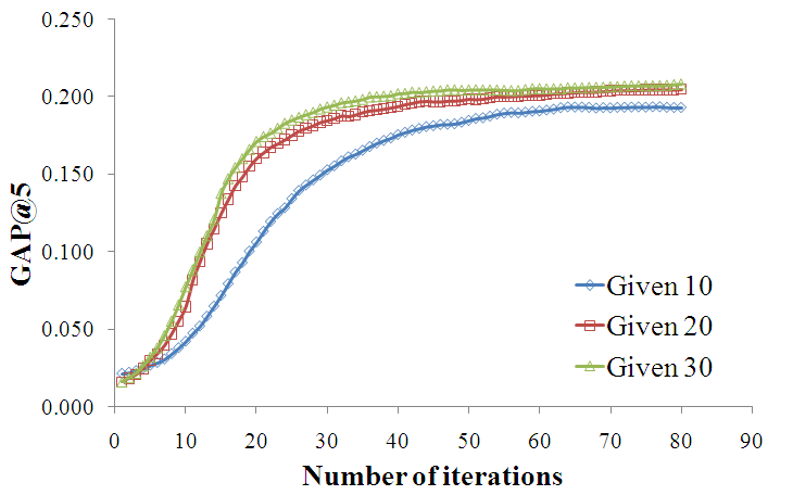
Figure 1: The Effectiveness of GAPfm.

5.3 Validation: Scalability

We conduct three experiments to validate the scalability of GAPfm. In the first experiment we empirically investigate the benefits that we can draw from employing parallel computing for updating latent user factors in GAPfm. We then validate the overall complexity of GAPfm as theoretically analyzed in Section 4.2. The last experiment is conducted to investigate the impact of the proposed adaptive selection strategy, as discussed in Section 4.3.

5.3.1 Parallel Updating of Latent User Factors

As shown in Section 4.2, the update of latent user factors $U$ in GAPfm can be conducted in parallel. By utilizing multiple cores/processors of the computing machine for the experiments, we empirically investigate the average runtime for updating $U$ per iteration against the number of processors employed. Note that updating $U$ in parallel has no influence on the quality of the resulting latent factors, and thus, the performance of the recommendation lists is not influenced. As shown in Fig. 2, for each of the “Given” conditions, the runtime of updating $U$ in the learning algorithm is reduced remarkably when increasing the number of processors for parallelizing the learning process. Note that the reduction of runtime for updating $U$ is not exactly inversely-proportionate to the number of processors, due to the system process maintenance constraints. However, the experiments are sufficient to demonstrate that parallelization can be used to speedup the optimization of the latent user factors in GAPfm, given adequate computing facilities.

Figure 2: The runtime of updating $U$ in parallel in the learning algorithm of GAPfm.

5.3.2 Linear Complexity

Since the size of the data used for training the latent factors in GAPfm varies under different “Given” conditions, we can empirically measure the complexity of GAPfm by observing the computational time consumed at each condition. In Fig. 3, the average iteration time is shown, which grows nearly linearly as the number of ratings used for training increases. This result validates the scalability of GAPfm under the basic setting, i.e., it scales linearly to the amount of observed data in the training dataset.

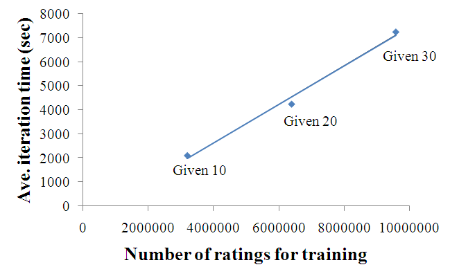
Figure 3: The relationship of the average iteration time against the size of data for training GAPfm.

5.3.3 Impact of Adaptive Selection

In order to investigate the impact of the adaptive selection strategy for GAPfm, we design an experiment under the condition of “Given 50" to measure the computational cost for the cases where different numbers of items, i.e., different values for $K$ (varying from 5 to 50), are adaptively selected during iterations for each user for training GAPfm. Meanwhile, we measure the performance of GAP based on the hold-out data in the validation set, corresponding to each case of $K$.

The results are shown in Fig. 4. Note that increasing $K$ is equivalent to increasing the size of the data for training GAPfm. Thus, as shown in the previous experiment, the average iteration time increases almost linearly to the growth of $K$. However, we do observe that GAPfm already achieves relatively high GAP even with a small value of $K$, compared to the GAP achieved when the latent factors of all the items (i.e., $K=50$) are updated. For instance, when only 20 items are adaptively selected for updating their latent factors in each iteration of the learning algorithm, i.e., $K=20$, nearly 75% of the runtime can be saved, compared to the case of updating the latent factors of all the items. Meanwhile, the drop of GAP is only around 5%, i.e., the GAP is 0.206 when $K=20$, and 0.216 when $K=50$. For large-scale datasets where computational cost is crucial, the small performance hit introduced by the adaptive selection process pays off due to the large gain attained in terms of computational cost. As analyzed in Section 4.3, we can practically maintain a constant complexity of GAPfm by using adaptive selection with a fixed $K$. In next section, we will further demonstrate the performance of GAPfm with adaptive selection in the case of $K=20$. Finally, we also conducted an experiment for validating the utility of adaptive selection, compared to random selection, i.e., in the case of $K=20$ we randomly select 20 rated items for updating their latent factors in each iteration of GAPfm. Random selection for $K=20$ produced a value of GAP = 0.166, which is 19% lower than computed using adaptive selection. In total, the experimental results confirm the value of the proposed adaptive selection for GAPfm in terms of both recommendation performance and the computational cost.

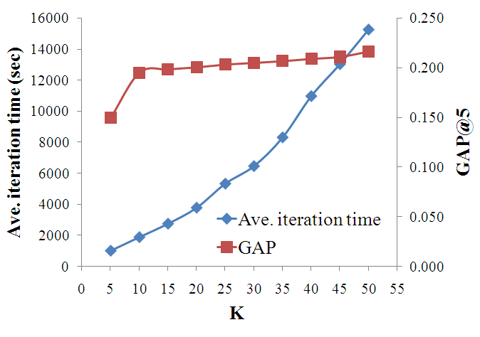
Figure 4: The impact of value $K$ on both the computational cost and the performance of GAP.

Summarizing, the observations from the experiments presented above allow us to give a positive answer to our second research question, i.e., GAPfm can be highly scalable (with constant complexity independent of the scale of the given dataset) and used for large-scale datasets.

Table 2: Performance comparison of GAPfm and the baseline approaches on the Netflix dataset.

		Given 10			Given 20			Given 30
	P@5	NDCG@5	GAP@5	P@5	NDCG@5	GAP@5	P@5	NDCG@5	GAP@5
PopRec	0.023	0.080	0.165	0.024	0.084	0.171	0.026	0.085	0.176
SVD++	0.023	0.065	0.133	0.027	0.071	0.139	0.032	0.087	0.168
CofiRank	0.027	0.093	0.181	0.027	0.088	0.182	0.025	0.088	0.186
GAPfm	0.040	0.109	0.195	0.042	0.111	0.207	0.042	0.114	0.213

5.4 Performance on Top-N Recommendation

We compare the performance of GAPfm with three baseline approaches. Each of the baseline approaches is listed and briefly introduced below:

• PopRec is a naive and non-personalized baseline that recommends movies in terms of their popularity, i.e., the number of ratings from all the users. Note that another naive baseline based on the average rating of movies was also tested, but it achieved rather low performance compared to other baselines. For this reason, we excluded it from our experimental results reported in this paper. Although being a naive baseline, PopRec is shown in literature to have competitive performance for the top-N recommendation task on the Netflix dataset [8].

• SVD++ is a state-of-the-art CF approach, which is shown to be superior for the rating prediction task as witnessed in the Netflix Prize contest [18]. We use the implementation of SVD++ available in GraphLab [23]. Note that the dimensionality of latent factors used in SVD++ is set to 10, the same as the setting for the proposed GAPfm. Other parameters, such as the regularization parameter, are tuned according to the observation from the validation set.

• CofiRank is a state-of-the-art CF approach that specifically optimizes for the ranking performance of recommendation results [36]. In addition, to the best of our knowledge, CofiRank is also the only well-established CF approach that directly optimizes NDCG measure for graded relevance datasets. Note that the implementation of CofiRank is based on the publicly available software package from the authors. The dimensionality of latent factors is also set to 10, and the remaining parameters are tuned on the validation set.

In Table 2, we present the performance of GAPfm and the baseline approaches for “Given” 10 to 30 items per user in the training set. Under all three conditions, GAPfm largely outperforms all the baselines, i.e., over 30% in P@5, 15% in NDCG@5 and 10% in GAP@5. All the improvements are statistically significant, according to Wilcoxon signed rank significance test with p<0.01. The results indicate that the proposed GAPfm is highly competitive for the top-N recommendation task. We also demonstrate that the optimization of GAP leads to improvements in terms of precision and NDCG. We also notice that SVD++ is only slightly better than PopRec in P@5 (which was also observed in related work of  [8]), but worse than PopRec in both NDCG@5 and GAP@5. This result again indicates that optimizing rating predictions do not necessarily lead to good performance for top-N recommendations.

In Table 3, we show the performance of GAPfm with adaptive selection for “Given 50” items per user in the training set, which simulates the case of relatively large user profiles. As indicated in Section 5.3, we adopt $K=20$ for the adaptive selection in GAPfm. GAPfm still achieves a large improvement over all of the baselines across all the metrics, and also slightly outperforms GAPfm with adaptive selection, i.e., ca. 6% in NDCG@5 and ca. 8% in GAP@5. However, we observe that GAPfm with adaptive selection still improves over PopRec, SVD++ and CofiRank to a significant extent. Moreover, as mentioned before, under the condition of “Given 50", training GAPfm with adaptive selection at $K=20$ saves around 75% computation time. Therefore, the drop in recommendation performance can be considered to be acceptable for real-world applications.

Table 3: Performance of GAPfm with adaptive selection ($K=20$) on the Netflix dataset under the condition “Given 50”

	P@5	NDCG@5	GAP@5
PopRec	0.025	0.085	0.172
SVD++	0.031	0.080	0.150
CofiRank	0.023	0.084	0.188
GAPfm	0.044	0.122	0.219
GAPfm+Adaptive Selection	0.044	0.115	0.201

Table 4: NDCG performance of GAPfm compared to WLT on the MovieLens 100K dataset

		Given 10			Given 20			Given 30			Given 40
	@1	@3	@5	@1	@3	@5	@1	@3	@5	@1	@3	@5
WLT	0.710	0.683	0.680	0.703	0.695	0.692	0.714	0.712	0.710	0.741	0.719	0.715
GAPfm	0.709	0.692	0.683	0.717	0.691	0.695	0.722	0.709	0.708	0.736	0.712	0.704

5.5 Performance on Ranking Graded Items

The last experiment is conducted to examine the performance of GAPfm on the task of ranking a given list of rated/graded items. We compare GAPfm with other collaborative ranking approaches proposed in the literature. Note that our focus on this paper is on top-N recommendation, which differs essentially from the ranking of rated items. In this setting we do not sample unrated items but only focus on the correct ranking of the rated items. However, this experiment only serves to verify that GAPfm would be still competitive even in the case of evaluating the ranking of rated items. For this reason, we extend our experiment on a different dataset, i.e., the MovieLens 100K dataset [12], and compare the performance of GAPfm with a state-of-the-art approach, Win-Loss-Tie (WLT) feature-based collaborative ranking [33], which is, to our knowledge, the latest contribution to collaborative ranking. We follow exactly the same experimental protocol as used in the work of [33], to allow us to make a straightforward comparison with the results reported in their work. The results are shown in Table 4. We observe that GAPfm achieves competitive performance for ranking rated items, across all the conditions and NDCG at all the truncation levels. These results indicate that the optimization of GAP for top-N recommendation would naturally lead to improvements in terms ranking graded items.

In summary, according to our observations from Section 5.4 and 5.5, we can conclude a positive answer to our last research question.

6 Conclusions and future work

We have presented GAPfm, a new CF approach for top-N recommendation, by learning a latent factor model that directly optimizes GAP. We propose an adaptive selection strategy for GAPfm so that it could attain a constant computational complexity, which guarantees its usefulness for large scale use scenarios. Our experiments also empirically validate the scalability of GAPfm. GAPfm is demonstrated to substantially outperform the baseline approaches for the top-N recommendation task, while also being competitive for the performance of ranking graded items, compared to the state of the art.

There are a few directions for future work. First, inspired by statistical analysis of evaluation metrics [35], we would like to analyze the relations and differences between learning methods that optimize different evaluation metrics. Second, we are also interested in developing distributed version of the proposed GAPfm, by taking into account recent contributions of distributed latent factor models [10]. Third, considering the multi-facet relevance judgments in recommender systems, such as accuracy, diversity, serendipity, we would also like to investigate the possibilities of optimizing top-N recommendation with multiple cohesive or competing objectives [3, 16, 30].

Appendix A Validation of Eq. (7)

Note that we neglect the user index $m$ in the following, due to its irrelevance to this validation. Given relevance predictions on all the items, i.e., $f_{i}$, $i=1,2,\ldots,N$, the definition of the rank of item $i$, i.e., $R_{i}$, can be formulated as below:

$$R_{i}=1+\sum_{j=1}^{N}\mathbb{I}(f_{i}<f_{j})$$

Suppose that $f$ is continuous and bounded within $[a,b]$. We can approximate $R_{i}$ by a smooth function of $f$ as below:

$$R_{i}\approx 1+\sum_{j=1}^{N}\frac{e^{f_{j}-f_{i}}}{e^{b}}=1+\frac{e^{-f_{i}}}{e^{b}}\sum_{j=1}^{N}e^{f_{j}}$$

In the case $N$ is large (which is common for most recommendation domains), we could further approximate the summation by integration over all the possible values of $f$. Under this approximation, we obtain:

$$R_{i} \approx 1+\frac{e^{-f_{i}}}{e^{b}}\int_{a}^{b}e^{f}\textup{d}f=1+\frac{e^{-f_{i}}}{e^{b}}(e^{b}-e^{a})$$

$$=1+(1-e^{-(b-a)})e^{-f_{i}}$$

Note that it is reasonable to assume $b-a>>0$, since theoretically $b$ could be positive infinite and $a$ could be negative infinite (if latent factors are drawn from real values). Therefore, we can finally obtain:

$$R_{i}\approx 1+e^{-f_{i}}$$

which validates the approximation in Eq. (7), i.e., $1/R_{i}=g(f_{i})$.

Appendix B Derivation of Eq. (11)

Note that we drop the derivative of the regularization term, i.e., $-\lambda V_{i}$ in the following.

$$\frac{\partial F}{\partial V_{i}} =I_{mi}g^{\prime}(f_{mi})U_{m}\sum_{j=1}^{N}I_{mj}\beta_{mij}g(f_{m(j-i)})$$

$$+I_{mi}g(f_{mi})\sum_{j=1,j\neq i}^{N}I_{mj}\beta_{mij}g^{\prime}(f_{m(j-i)})(-U_{m})$$

$$+\sum_{k=1,k\neq i}^{N}I_{mk}g(f_{mk})I_{mi}\beta_{mki}g^{\prime}(f_{m(i-k)})U_{m}$$

Replacing $k$ with $j$ in the last summation term, and applying the property $g^{\prime}(-x)=g^{\prime}(x)$ so as to combine the last two summation terms, we obtain:

$$\frac{\partial F}{\partial V_{i}} =I_{mi}g^{\prime}(f_{mi})U_{m}\sum_{j=1}^{N}I_{mj}\beta_{mij}g(f_{m(j-i)})$$

$$+U_{m}\sum_{j=1,j\neq i}^{N}I_{mi}I_{mj}\big{(}\beta_{mji}g(f_{mj})-\beta_{mij}g(f_{mi})\big{)}g^{\prime}(f_{m(j-i)})$$

Note that $\beta_{mji}g(f_{mj})-\beta_{mij}g(f_{mi})=0$ if $i=j$. We can add this condition into above and take out $I_{mi}$ and $U_{m}$ to attain Eq. (4.2).

Appendix C Adaptive Selection

We present our justification of the criterion for adaptive selection proposed in Section 4.3. Note that in the following, we drop the user index $m$, due to its irrelevance to this validation. By the definition of the indicator function $\mathbb{I}$, we have $\mathbb{I}(y_{i}<y_{j})+\mathbb{I}(y_{j}\leq y_{i})=1$. Therefore, we can rewrite Eq. (4) as:

$$\beta_{ij}: =\big{(}1-\mathbb{I}(y_{j}\leq y_{i})\big{)}\sum_{l=1}^{y_{i}}\delta_{l}+\mathbb{I}(y_{j}\leq y_{i})\sum_{l=1}^{y_{j}}\delta_{l}$$

$$=\sum_{l=1}^{y_{i}}\delta_{l}+\big{(}\sum_{l=1}^{y_{j}}\delta_{l}-\sum_{l=1}^{y_{i}}\delta_{l}\big{)}\mathbb{I}(y_{j}\leq y_{i})$$

Substituting above equation into Eq. (3), we obtain:

$$GAP= \sum_{i=1}^{N}\frac{I_{i}\sum_{l=1}^{y_{i}}\delta_{l}}{R_{i}}\sum_{j=1}^{N}I_{j}\mathbb{I}(R_{j}\leq R_{i})$$

$$+\sum_{i=1}^{N}\frac{I_{i}}{R_{i}}\sum_{j=1}^{N}I_{j}\mathbb{I}(R_{j}\leq R_{i})\mathbb{I}(y_{j}\leq y_{i})\big{(}\sum_{l=1}^{y_{j}}\delta_{l}-\sum_{l=1}^{y_{i}}\delta_{l}\big{)}$$

Note that the first summation is non-negative. Also note that when $R_{j}\leq R_{i}$ and $y_{j}\leq y_{i}$ (i.e., two items are misranked), we have $\sum_{l=1}^{y_{j}}\delta_{l}-\sum_{l=1}^{y_{i}}\delta_{l}\leq 0$. Therefore, the second summation is composed by non-positive terms, i.e., only leading to a loss of GAP. In addition, the loss is proportionate to $\sum_{l=1}^{y_{j}}\delta_{l}-\sum_{l=1}^{y_{i}}\delta_{l}$, the difference of grades of misranked items. Thus, it is obvious that the largest loss would be casued by the most misranked item, justifying our criterion for adaptive selection, i.e., updating most misranked items would lead to largest upgrade of GAP.

Appendix D Characteristics of GAPfm

Generalization. In the scenario with implicit feedback data (binary relevance data), we have $y_{max}=1$. Thus, in the case of $I_{mi}>0$ and $I_{mj}>0$, it implies that we have $y_{mi}=y_{mj}=y_{max}=1$. Substituting this condition into Eq. (4) and taking into account of the definition of in Eq. (5), we obtain $\beta_{mij}=1$. Furthermore, the smoothed GAP as in Eq. (8) returns to:

$$GAP_{m}=\sum_{i=1}^{N}I_{mi}g(f_{mi})\sum_{j=1}^{N}I_{mj}g(f_{m(j-i)})$$

which is equivalent to the smoothed AP (excluding the context variable and the constant coefficient) as proposed in the work of [28]. Therefore, the proposed GAPfm is a generalization of the approach optimizing AP in the implicit feedback domains.

Specialization. Graded precision and graded recall are two specialized metrics that can be decomposed from GAP. As defined in [26], we can rewrite GP@n and GR@n for the top-n recommendation list of user $m$ as follows:

$$GP_{m}@n=\frac{1}{n}\sum_{i=1}^{N}I_{mi}\mathbb{I}(R_{mi}\leq n)\xi_{mi}^{(n)}$$

$$GR_{m}@n=\frac{1}{Z_{m}}\sum_{i=1}^{N}I_{mi}\sum_{l=1}^{y_{mi}}\delta_{l}\mathbb{I}(R_{mi}\leq n)$$

where,

$$\xi_{mi}^{(n)}:=\frac{\mathbb{I}(y_{mi}<c_{mn})\sum_{l=1}^{y_{mi}}\delta_{l}+\mathbb{I}(c_{mn}\leq y_{mi})\sum_{l=1}^{c_{mn}}\delta_{l}}{\sum_{j=1}^{c_{mn}}\delta_{l}}$$

$c_{mn}$ denotes the grade of the $n$th item in the user $m$’s ranked list, according the descending order of her rated items. We may attain smoothed versions of GP@n and GR@n by approximating $\mathbb{I}(R_{mi}\leq n)$ with smoothed functions of latent factors $U$ and $V$, such as

$$\mathbb{I}(R_{mi}\leq n)\approx g(\left\langle U_{m},V_{i}\right\rangle-c_{mn})$$

Then, similar optimization as used in GAPfm can be performed to learned latent factors that optimize GP@n or GR@n.

References

- [1] G. Adomavicius and A. Tuzhilin. Toward the next generation of recommender systems: A survey of the state-of-the-art and possible extensions. IEEE Transactions on Kowledge and Data Engineering, 17(6):734–749, 2005.
- [2] D. Agarwal and B.-C. Chen. Regression-based latent factor models. KDD ’09, pages 19–28. ACM, 2009.
- [3] D. Agarwal, B.-C. Chen, P. Elango, and X. Wang. Personalized click shaping through lagrangian duality for online recommendation. SIGIR ’12, pages 485–494. ACM, 2012.
- [4] S. Balakrishnan and S. Chopra. Collaborative ranking. WSDM ’12, pages 143–152. ACM, 2012.
- [5] C. J. C. Burges, R. Ragno, and Q. V. Le. Learning to rank with nonsmooth cost functions. NIPS ’06, pages 193–200, 2006.
- [6] O. Chapelle, D. Metlzer, Y. Zhang, and P. Grinspan. Expected reciprocal rank for graded relevance. In Proceedings of the 18th ACM conference on Information and knowledge management, CIKM ’09, pages 621–630, New York, NY, USA, 2009. ACM.
- [7] O. Chapelle and M. Wu. Gradient descent optimization of smoothed information retrieval metrics. Inf. Retr., 13:216–235, June 2010.
- [8] P. Cremonesi, Y. Koren, and R. Turrin. Performance of recommender algorithms on top-n recommendation tasks. RecSys ’10, pages 39–46. ACM, 2010.
- [9] M. D. Ekstrand, J. T. Riedl, and J. A. Konstan. Collaborative filtering recommender systems. Foundations and Trends in Human-Computer Interaction, 4(2):81–173, 2011.
- [10] R. Gemulla, E. Nijkamp, P. J. Haas, and Y. Sismanis. Large-scale matrix factorization with distributed stochastic gradient descent. KDD ’11, pages 69–77. ACM, 2011.
- [11] A. Gunawardana and G. Shani. A survey of accuracy evaluation metrics of recommendation tasks. J. Mach. Learn. Res., 10:2935–2962, December 2009.
- [12] J. L. Herlocker, J. A. Konstan, A. Borchers, and J. Riedl. An algorithmic framework for performing collaborative filtering. SIGIR ’99, pages 230–237. ACM, 1999.
- [13] T. Hofmann. Latent semantic models for collaborative filtering. ACM Trans. Inf. Syst., 22:89–115, January 2004.
- [14] L. Hong, R. Bekkerman, J. Adler, and B. D. Davison. Learning to rank social update streams. SIGIR ’12, pages 651–660. ACM, 2012.
- [15] Y. Hu, Y. Koren, and C. Volinsky. Collaborative filtering for implicit feedback datasets. ICDM ’08, pages 263–272. IEEE Computer Society, 2008.
- [16] T. Jambor and J. Wang. Optimizing multiple objectives in collaborative filtering. RecSys ’10, pages 55–62. ACM, 2010.
- [17] K. Järvelin and J. Kekäläinen. Cumulated gain-based evaluation of ir techniques. ACM Trans. Inf. Syst., 20(4):422–446, Oct. 2002.
- [18] Y. Koren. Factorization meets the neighborhood: a multifaceted collaborative filtering model. KDD ’08, pages 426–434. ACM, 2008.
- [19] Y. Koren, R. Bell, and C. Volinsky. Matrix factorization techniques for recommender systems. Computer, 42:30–37, August 2009.
- [20] N. N. Liu and Q. Yang. Eigenrank: a ranking-oriented approach to collaborative filtering. SIGIR ’08, pages 83–90. ACM, 2008.
- [21] N. N. Liu, M. Zhao, and Q. Yang. Probabilistic latent preference analysis for collaborative filtering. CIKM ’09, pages 759–766. ACM, 2009.
- [22] T.-Y. Liu. Learning to rank for information retrieval. Foundations and Trends in Information Retrieval, 3(3):225–331, 2009.
- [23] Y. Low, J. Gonzalez, A. Kyrola, D. Bickson, C. Guestrin, and J. M. Hellerstein. Distributed graphlab: A framework for machine learning in the cloud. PVLDB, 5(8):716–727, 2012.
- [24] C. D. Manning, P. Raghavan, and H. Schütze. Introduction to information retrieval. Cambridge Univ. Press, Cambridge [u.a.], 1. publ. edition, 2008.
- [25] S. Rendle, C. Freudenthaler, Z. Gantner, and S.-T. Lars. Bpr: Bayesian personalized ranking from implicit feedback. UAI ’09, pages 452–461. AUAI Press, 2009.
- [26] S. E. Robertson, E. Kanoulas, and E. Yilmaz. Extending average precision to graded relevance judgments. SIGIR ’10, pages 603–610. ACM, 2010.
- [27] B. Sarwar, G. Karypis, J. Konstan, and J. Reidl. Item-based collaborative filtering recommendation algorithms. WWW ’01, pages 285–295. ACM, 2001.
- [28] Y. Shi, A. Karatzoglou, L. Baltrunas, M. Larson, A. Hanjalic, and N. Oliver. TFMAP: optimizing map for top-n context-aware recommendation. SIGIR ’12, pages 155–164. ACM, 2012.
- [29] Y. Shi, A. Karatzoglou, L. Baltrunas, M. Larson, N. Oliver, and A. Hanjalic. CLiMF: learning to maximize reciprocal rank with collaborative less-is-more filtering. RecSys ’12, pages 139–146. ACM, 2012.
- [30] K. M. Svore, M. N. Volkovs, and C. J. Burges. Learning to rank with multiple objective functions. WWW ’11, pages 367–376. ACM, 2011.
- [31] M. Taylor, J. Guiver, S. Robertson, and T. Minka. Softrank: optimizing non-smooth rank metrics. WSDM ’08, pages 77–86. ACM, 2008.
- [32] I. Tsochantaridis, T. Joachims, T. Hofmann, and Y. Altun. Large margin methods for structured and interdependent output variables. J. Mach. Learn. Res., 6:1453–1484, 2005.
- [33] M. N. Volkovs and R. S. Zemel. Collaborative ranking with 17 parameters. NIPS ’12, 2012.
- [34] E. M. Voorhees. The trec-8 question answering track report. In TREC-8, 1999.
- [35] J. Wang and J. Zhu. On statistical analysis and optimization of information retrieval effectiveness metrics. SIGIR ’10, pages 226–233. ACM, 2010.
- [36] M. Weimer, A. Karatzoglou, Q. Le, and A. Smola. Cofirank - maximum margin matrix factorization for collaborative ranking. NIPS’07, pages 1593–1600, 2007.
- [37] J. Xu and H. Li. Adarank: a boosting algorithm for information retrieval. SIGIR ’07, pages 391–398. ACM, 2007.
- [38] J. Xu, T.-Y. Liu, M. Lu, H. Li, and W.-Y. Ma. Directly optimizing evaluation measures in learning to rank. SIGIR ’08, pages 107–114. ACM, 2008.
- [39] S.-H. Yang, B. Long, A. J. Smola, H. Zha, and Z. Zheng. Collaborative competitive filtering: learning recommender using context of user choice. SIGIR ’11, pages 295–304. ACM, 2011.
- [40] Y. Yue, T. Finley, F. Radlinski, and T. Joachims. A support vector method for optimizing average precision. SIGIR ’07, pages 271–278. ACM, 2007.