Quantum simulations of a particle in one-dimensional potentials using NMR

Abstract

A classical computer simulating Schrodinger dynamics of a quantum system requires resources which scale exponentially with the size of the system, and is regarded as inefficient for such purposes. However, a quantum computer made up of a controllable set of quantum particles has the potential to efficiently simulate other quantum systems of matching dimensions. In this work we studied quantum simulations of single particle Schrodinger equation for certain one-dimensional potentials. In particular, we report the following cases: (i) spreading of wave-function of a free-particle, (ii) evolution of a particle in a potential-well, and (iii) reflection of a particle from a potential-barrier. Using a five-qubit NMR system, we achieve space discretization with four qubits, and the other qubit is used for preparation of initial states as well as measurement of spatial probabilities. The experimental relative probabilities compare favourably with the theoretical values, thus effectively mimicking a small-scale quantum simulator.

I Introduction

We have reached a stage in digital computing, conforming to Moore’s law, where quantum effects are more pronounced and serve as a hindrance to transistor performance Moore et al. (1965). The way forward, as Feynman suggested, is to use these effects to our advantage in building a computer - a quantum computer Feynman (1982). The fundamental working of any quantum computer, if built, boils down to initializing a quantum state, transforming it by a desired unitary operator, and finally performing an efficient readout of the final state. It has been established theoretically that quantum computers have the capability to alter the complexity of certain computational problems from exponentials to polynomials. A well-known example is Shor’s algorithm for prime-factorization Shory (1995). Another important example is simulating the dynamics of quantum systems Feynman (1982). Dynamics of a quantum particle in a potential is governed by Schrodinger equation. Simulating the dynamics is carried out by assigning a state vector to the system, and transforming it using unitary operators. For a system consisting of $n$ mutually interacting spin-1/2 particles the dimension of the state vector increases as $2^{n}$ and that of unitary operator as $2^{n}\times 2^{n}$. Thus the number of variables in the problem increases exponentially with the size of the system. Nevertheless, as Feynman noted, a quantum system can be efficiently simulated with the help of another controllable quantum system - a quantum simulator Feynman (1982); Buluta and Nori (2009).

Extensive studies have been made on quantum simulations using both theory and experiments. After Feynman popularized the concept of quantum simulators, the idea was further studied by Lloyd and Braunstein Lloyd (1996); Lloyd and Braunstein (1999). Later quantum simulations of various problems were investigated in detail. For example, Farhi et al have studied simulations of quantum walk Farhi and Gutmann (1998). Cory and co-workers have simulated the dynamics of truncated quantum harmonic and anharmonic oscillators using nuclear magnetic resonance (NMR) Havel et al. (2002). Laflamme and co-workers have simulated quantum many-body problems using similar techniques Negrevergne et al. (2005). Wineland and co-workers have realized an ion-trap quantum simulator and demonstrated its application as a non-linear interferometer Leibfried et al. (2002). Jingfu et al have simulated a perfect state transfer in spin chains using Heisenberg XY interactions on an NMR system Zhang et al. (2005). White and co-workers have simulated molecular hydrogen and experimentally obtained its energy spectrum using photonic quantum computer technology Lanyon et al. (2010). Du and co-workers have also obtained the ground state energy of hydrogen molecule by an NMR quantum simulator Du et al. (2010). Oliveira and co-workers have simulated magnetic phase transitions by writing electronic states of a ferromagnetic system onto nuclear spin states Soares-Pinto et al. (2011). More recently, Koteswara et al have used an NMR quantum simulator to establish multipartite quantum correlations as an indicator of frustration in Ising spin system Rao et al. (2013). The applications of spin-qubits as quantum simulators are discussed in a review by Peng and Suter Suter et al. (2010).

In this article we report the experimental demonstration of time-evolution of a quantum particle under various potentials using NMR techniques on a 5-qubit system. As described in the next section, the quantum simulation of a particle in a potential can be decomposed into two parts: the evolution under potential energy in position basis, and the evolution under kinetic energy in momentum basis. The change of basis is achieved by Fourier transform and finally the probabilities are measured in the position basis. In our work, we utilize four qubits to discretize the position space. We also utilize an ancilla qubit to (i) prepare an initial state and (ii) directly encode the spatial probabilities onto the ancilla spectral lines. Therefore the need of a quantum state tomography and associated post-processing of data, is avoided.

In the following section we outline the theory of quantum simulations of a particle in a one-dimensional potential. In section III we describe the experimental methods in simulating a few potentials and discuss the results. Finally we conclude in section IV.

II Theory

The dynamics of a quantum particle of mass $\mu$ in a one-dimensional potential $V(x)$ is governed by the time-dependent Schrodinger equation,

$$i\hbar\frac{\partial|{\psi}\rangle}{\partial t}={\cal H}|{\psi}\rangle,$$ (1)

where $|{\psi}\rangle$ is the state vector and

$${\cal H}={\cal H}_{0}+V(x)$$ (2)

is the Hamiltonian in position basis ($x$-basis). Here ${\cal H}_{0}=\frac{-\hbar^{2}}{2\mu}\frac{\partial^{2}}{\partial x^{2}}$ represents the kinetic part of the Hamiltonian. The mass $\mu$ and the reduced Planck’s constant $\hbar$ are set to unity from here onwards. Further we use the position basis to encode the initial state and to measure the probabilities of the final state. If the system is represented by an initial wave-function $\psi(x,t)$ at a time instant $t$, after an evolution over a small time duration $\delta t$, the wave-function is given by

$$\psi(x,t+\delta t)=e^{-i{\cal H}\delta t}\psi(x,t).$$ (3)

We choose a domain of length $L$ to which the spread of the wave-function is confined in $x$-basis. We utilize an $n$-qubit register to encode discrete positions

$$x_{j}=x_{0}+j\Delta x.$$ (4)

Here the index $j$ runs from 0 to $N-1$, with $N=2^{n}$, $x_{0}=-L/2$ and $x_{N-1}=+L/2$ forming the terminals, and the resolution of discretization, $\Delta x=L/(N-1)$, is limited by the size of the register. The state vector can now be expressed in position basis as

$$|{\psi(t)}\rangle=\frac{1}{\sqrt{N}}\sum_{j=0}^{N-1}\psi(x_{j},t)|{j}\rangle$$ (5)

where $\{|{j}\rangle\}$ represents the computational basis formed by the $n$-qubit register Benenti and Strini (2008).

Since the two parts, ${\cal H}_{0}$ and $V$, of the Hamiltonian do not commute, one can utilize Trotter’s formula

$$e^{-i{\cal H}\delta t}=e^{-iV\delta t/2}e^{-i{\cal H}_{0}\delta t}e^{-iV\delta t/2}+O(\delta t^{3})$$ (6)

to decompose the total evolution over a duration $\delta t$ into independent evolutions under potential and kinetic parts.

In the discretized position basis, the evolution under the potential part $V(x)$ leads to the transformed wave-function $e^{-iV(x_{j})\delta t}\psi(x_{j},t)$. This is equivalent to applying a diagonal unitary operator to the state-vector. Such a transformation can be implemented efficiently on a quantum computer Nielsen and Chuang (2010); Benenti and Strini (2008). However, the second part, i.e., the kinetic energy part in the Hamiltonian (Eq. [2]) is non-diagonal in the position basis, and has no efficient decomposition. The trick involves applying discrete Fourier transform ${\cal F}$ to transform the wave-function into momentum basis Boashash (2003), i.e.,

$$\widetilde{\psi}(k_{l},t)=\frac{1}{\sqrt{2\pi}}\sum_{j=0}^{N-1}\psi(x_{j},t)e^{ik_{l}x_{j}}\Delta x.$$ (7)

In the discretized momentum basis ($k$-basis),

$$k_{l}=k_{0}+l\Delta k$$ (8)

is the $l$th point, with $\Delta k=2\pi/L$, and $k_{0}=-(N-1)\Delta k/2$ and $k_{N-1}=+(N-1)\Delta k/2$ forming the terminals. In this basis, the kinetic-energy part $\widetilde{\cal H}_{0}$ becomes diagonal, i.e., $\langle{k_{j}}|{\widetilde{\cal H}_{0}}|{k_{l}}\rangle=\delta_{jl}k_{l}^{2}/2$, where $\delta_{jl}$ is the Kronecker delta function. Therefore the transformed wave-function is of the form $e^{-i(k_{l}^{2}/2)\delta t}\widetilde{\psi}(k_{l},t)$. Again the methods of efficient decompositions can be used to apply the diagonal operator Wiesner (1996); Zalka (1998); Strini (2002); Benenti and Strini (2008).

Thus the net evolution over a small duration $\delta t$ can be approximated as

$$e^{-i{\cal H}\delta t}\approx e^{-iV\delta t/2}{\cal F}^{-1}e^{-i\widetilde{\cal H}_{0}\delta t}{\cal F}e^{-iV\delta t/2}.$$ (9)

Hence a single time-step ($\delta t$) evolution of $|{\psi}\rangle$ is achieved by the application of operators $U_{V}=e^{-iV\delta t/2}$, ${\cal F}$, $\widetilde{U}_{0}=e^{-i\widetilde{\cal H}_{0}\delta t}$, and ${\cal F}^{-1}$ in the sequence given above.

In the next section we describe the experimental methods employed for the quantum simulations of certain one-dimensional potentials and discuss the results obtained.

III Experiments

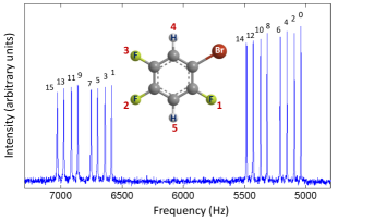
Figure 1: Molecular structure of 1-bromo-2,4,5-trifluorobenzene and ¹⁹F spectrum of F₁ spin. The state labels ($|{j}\rangle$) shown at the top of each transition are obtained through Z-COSY experiments and are consistent with the spin-states of the register (qubits 2 to 5).

In our experiments we utilize three ¹⁹F spins and two ¹H spins of 1-bromo-2,4,5-trifluorobenzene partially oriented in liquid crystal N-(4-methoxybenzaldehyde)-4-butylaniline (MBBA). The molecular structure and the labelling of qubits are shown in the inset of Fig. 1. All the experiments are carried out on a 500 MHz Bruker UltraShield spectrometer at an ambient temperature of 300 K. The effective couplings in such a system is due to scalar interactions (J-couplings) as well as partially averaged dipolar interactions (DD-couplings). The values of resonance frequencies in a doubly rotating frame, longitudinal relaxation time constants (T₁), effective transverse relaxation time constants (T₂), and strengths of effective couplings ($D_{ij}$) are tabulated below:

Spin	$\nu_{i}$	$T_{1}$	$T_{2}^{*}$
number	(Hz)	(s)	(ms)
1	6029	0.7	65-125
2	-3680	0.4	45-65
3	-6743	0.5	45-65
4	50	1.4	150
5	29	1.3	150

$D_{ij}$ (Hz)
$D_{12}$ = 277	$D_{24}$ = 106
$D_{13}$ = 116	$D_{25}$ = 1270
$D_{14}$ = 54	$D_{34}$ = 1532
$D_{15}$ = 1556	$D_{35}$ = 55
$D_{23}$ = -26	$D_{45}$ = -7.6

As evident from the above table, all the 80 transitions in the oriented 5-spin system are fully resolved. We utilize the first qubit as ancilla and rest (i.e., qubits 2 to 5) as the four-qubit quantum register, whose computational states encode the 16 discrete points in position as well as momentum bases. Further, the ancilla has 16 well-resolved transitions, each of which corresponds to one particular qubit-state of the register (see Fig. 1).

Since the chemical shift difference $|\nu_{j}-\nu_{i}|$ in each pair of spins $(i,j)$ is much higher than the intra-pair effective coupling strength ($D_{ij}$), the Hamiltonian can be approximated to the form Cavanagh et al. (1995)

$${\cal H}_{\mathrm{int}}=-\pi\sum\limits_{i=1}^{n}\nu_{i}\sigma_{i}^{z}+\frac{\pi}{2}\sum\limits_{\begin{subarray}{c}i,j=1\\ i<j\end{subarray}}^{n}D_{ij}\sigma_{i}^{z}\sigma_{j}^{z}.$$ (10)

The first step in quantum simulation typically involves preparation of an initial pure state which is difficult using conventional NMR techniques. Instead a pseudopure state (PPS), with the density matrix

$$\rho(0) \ =\ \frac{1}{2^{n}}(1-\epsilon)\mathbbm{1}+\epsilon|\psi\rangle\langle\psi|,$$ (11)

isomorphous to a pure state $|{\psi}\rangle\langle{\psi}|$, can be prepared. There are a number of methods available for this purpose Cory et al. (1998); Knill et al. (1998); Mahesh and Kumar (2001); Knill et al. (2000); Roy and Mahesh (2010). Here we utilize the pair of pseudopure states (POPS) method described by Fung Fung (2001). In this method, as illustrated in Fig. 2, the full-system basis is divided into two sub-systems based on the ancilla states. The preparation consists of a pair of experiments, one starting from equilibrium population distribution $\{p_{i}\}$ (Fig. 2(a)), and the other starting from an initial distribution $\{q_{i}\}$ obtained by inverting a single transition of ancilla (Fig. 2(b)). Assuming linear response, the difference between the signals obtained in the two experiments corresponds to an initial state which is the difference of the initial population distributions, i.e., $\{p_{i}-q_{i}\}$ (Fig. 2(c)). For example, if the ancilla transition between the levels $|{00000}\rangle$ and $|{10000}\rangle$ is inverted, one obtains $|{0000}\rangle$ POPS (see Fig. 2(c)), which encodes the quantum system localized at position $|{j=0}\rangle$.

If the subsystems are not allowed to mix during the computation, (i.e., if no pulses are applied on the ancilla qubit) they undergo independent, simultaneous, and identical evolutions. Therefore the initial populations of the subsystems are redistributed within each subsystem in an identical manner (Fig. 2(d)), such that the differential deviation populations are same, but are of opposite signs in the two subsystems. In this work, the spatial probabilities are encoded by these differential populations $\{p_{i}-q_{i}\}$ and are reflected in the intensities of the ancilla spectral lines.

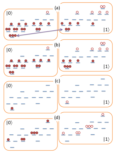
Figure 2: The energy-levels and representative deviation population distributions in the two subsystems corresponding to $|{0}\rangle$ and $|{1}\rangle$ states of the ancilla qubit. The filled circles indicate positive deviations (above the background population) and the empty circles indicate negative deviations (below the background population). Here following situations are illustrated (a) equilibrium distribution, (b) after inverting a transition (as shown in (a)), (c) difference between (a) and (b) forming a POPS, and (d) an example of intra-subsystem redistribution of the differential populations after applying an unitary (with identity on ancilla).

The pulse sequence for the simulation experiments are illustrated in Fig. 3. To measure the spatial probabilities after a time interval $\delta t$, we carry out two experiments (i) apply $e^{-i{\cal H}\delta t}$ to equilibrium state $\rho(0)$, destroy the transverse magnetization by using a pulsed field gradient (PFG), and read the signal by applying a linear detection pulse ($(\pi/2)_{y}^{1}$ pulse on ancilla) (see Fig. 3 (a)), and (ii) invert the desired ancilla transition, apply $e^{-i{\cal H}\delta t}$, destroy the transverse magnetization, and again read the signal by applying the linear detection pulse (see Fig. 3 (b)). The difference between the signals obtained in these two experiments directly encode the spatial probabilities. Thus the ancilla qubit provides a direct spectral information on the dynamics of the quantum system. In order to study the dynamics at a set of regularly spaced time instants, we repeat the evolution pulses shown in dashed boxes in Fig. 3.

The initial transition selective $\pi$ pulse in Fig. 3(b) is realized by a long Gaussian RF pulse of duration 30 ms. Other RF pulses used in the above pulse sequences are constructed using GRadient Ascent Pulse Engineering (GRAPE) technique and are designed to be robust against RF inhomogeneity. The operators shown in the dashed box, for each potential, in Fig. 3 are constructed as a single GRAPE pulse of duration 24 ms. The fidelities (averaged over inhomogeneous spatial distribution of RF amplitudes) of these pulses were better than 0.95. The final selective $(\pi/2)_{y}^{1}$ pulse on the ancilla was of duration 500 $\upmu$s and of average fidelity better than 0.99.

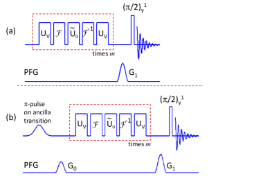
Figure 3: NMR pulse sequences used for simulating the quantum dynamics. The sequence (b) differs from (a) only by the initial transition selective inversion followed by a PFG (G₀). The PFG G₁ is used to destroy all the transverse magnetization before the final $(\pi/2)_{y}^{1}$ detection pulse on the ancilla. The operators in the dashed box, corresponding to the Schrodinger evolution, are repeated $m$ times to achieve an evolution over duration $m\delta t$.

We simulated the quantum dynamics of a particle starting from rest (with zero momentum expectation value) in the following three cases.

• Free-particle (Fig. 4): $V(x)=0$ for all values of $x$ in a lattice of length $L=8$. The particle starts from rest at $x=4/15$ ($j=8$ in Eq. (4)) and the evolution interval is $\delta t=\pi/20$.

• Particle in a well (Fig. 5): $V(x)=0$ for $-2/5\leq x\leq 2/15$ (i.e., $6\leq j\leq 8$), and $V(x)=60$ elsewhere in a lattice of length $L=4$. The particle starts from rest at $x=-2/15$ ($j=7$) and the evolution interval is $\delta t={\pi}/{100}$.

• Reflection from a barrier (Fig. 6): $V(x)=100$ at $2/5\leq x\leq 2/3$ (i.e., $9\leq j\leq 10$) and $V(x)=0$ elsewhere in a lattice of length $L=4$. The particle starts from rest at $x=-2/15$ ($j=7$) and the evolution interval is $\delta t={\pi}/{100}$.

It can be noticed that units of $V$ and $L$ are set by the conditions $\hbar=1$ and mass $\mu=1$. The parameter values in the above are chosen considering the contrast of spatial probabilities at different instants of time.

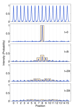
Figure 4: Top trace is the reference spectrum of ancilla obtained by rearranging normalized peaks from Fig. 1 in the increasing order of spectral labelling. Here position is in units of $\Delta x$. The spectra at $\delta t=0$ corresponds to the $|{j=8}\rangle$ POPS. Other spectra correspond to different evolution intervals as indicated. Shaded bars shown behind the spectral lines indicate expected probabilities.

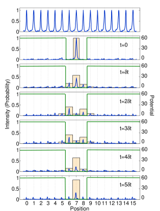
Figure 5: Reference spectrum (top trace) and spectra corresponding to the simulation of particle in a well for sequential intervals of time as indicated. The spectra at $\delta t=0$ corresponds to the $|{j=7}\rangle$ POPS. Shaded bars shown behind the spectral lines indicate expected probabilities. Potential is indicated by a solid line.

In the following we discuss each of these cases. For the case of free-particle, there is no need to apply $U_{V}$ mentioned in the pulse-sequence shown in Fig. 3. The GRAPE pulse implementing the propagator ${\cal F}^{-1}\widetilde{U}_{0}{\cal F}$ had an average fidelity of 0.98. The experimental results are shown in Fig. 4. The ancilla spectral lines normalized into equal intensities and ordered in the increasing values of transition-labels $(j)$ are shown in the top trace of Fig.4. These spectral lines are used as references for normalizing spectral lines in the other traces of the figure. The spectrum corresponding to $t=0$ is obtained from $|{j=8}\rangle$ POPS. The remaining traces show the spectra obtained after subsequent intervals of evolution (up to $3\delta t$). The expected spatial probabilities under an ideal reproduction of GRAPE pulses are shown as shaded bars behind the spectral lines. The spreading of the wave-function in zero-potential is clearly manifested in both theoretical and experimentally simulated plots. Ideally peak-heights of the spectral lines and the bars should match. Experimentally however, the spectral lines are generally of lower intensities as a result of decoherence. The overall duration of the pulse-sequence for simulating $3\delta t$ evolution is about 72 ms which is comparable to the $T_{2}$ values of the various spins in the molecule. Another major challenge is the gradual fluctuations in the residual dipolar couplings due to the local changes in the order parameter of the liquid crystal. This resulted not only in the line-broadening of spectral lines, but also temporal modulations in the Hamiltonian parameters. Other sources of errors like RF inhomogeneity, static-field inhomogeneity, and non-linear reproduction of the GRAPE pulses by the RF coils also contribute to the deviations of the experimental spectra from theory.

In order to compare the overall experimental performance with theory, we use the contour plots of the spatial probability with evolution time shown in Fig. 7 (a) and (b). Here the experimental contours (Fig. 7 (b)) are obtained by normalizing the sum of spectral intensities at each time-steps to unity, so that the effect of overall-decay is removed. Though the experimental contours deviate from theory (Fig. 7 (a)), the over-all pattern appears to match, indicating a satisfactory quantum simulation of the free-particle case. We use root-mean-square (RMS) errors to estimate the quality of the simulation (in a scale of 0 to 1). The RMS errors for various steps of evolution are plotted in Fig. 8. In the case of free-particle simulation, the maximum RMS error was less than 0.05.

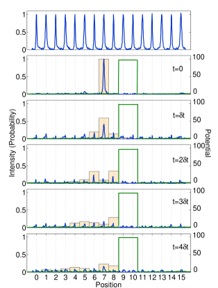
Figure 6: Reference spectrum (top trace) and spectra corresponding to the simulation of reflection from a barrier for sequential intervals of time as indicated. The spectra at $\delta t=0$ corresponds to the $|{j=7}\rangle$ POPS. Shaded bars shown behind the spectral lines indicate expected probabilities. Potential is indicated by a solid line.

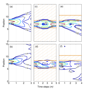
Figure 7: Theoretical (top row) and experimental (bottom row) contour plots showing time evolution of spatial probabilities in the case of (a,b) free-particle, (c,d) particle in a well, and (e,f) reflection from a barrier. Here position is in units of $\Delta x$ and time is in units of $m\delta t$. In plots (c)-(f), the patched areas correspond to non-zero values of potentials.

For the potential-well, the GRAPE evolution pulse had a lesser average fidelity of 0.95. Fig. 5 displays the results of simulations of particle in a well. Again the first trace is the reference and subsequent traces display the results corresponding to various evolution intervals. The initial state $|{j=7}\rangle$ is not a stationary state, but has a periodicity close to $5\delta t$. Comparison with the expected probabilities (shaded bars), indicates a gradual decay of the spectral lines, again due to decoherence. Comparison of the theoretical contours of probabilities in Fig. 7(c) with experimental contours in Fig. 7(d) indicates a fairly good simulation of the dynamics. Further, Fig. 8 indicates that RMS errors build up rapidly from the 4th step. However the overall experimental contour patterns in Fig. 7(d) reveal the $5\delta t$ periodicity as expected.

The GRAPE evolution pulse simulating reflection from a barrier also had a lesser average fidelity of 0.95. Fig. 6 displays the corresponding results. Again the initial state $|{j=7}\rangle$ is not a stationary state. As it spreads, it gets reflected from the barrier and is constrained to one side of the barrier. This phenomenon is evident in both the expected probabilities (shaded bars) as well as in the experimental spectral lines. The contours of probabilities in Fig. 7(e) and (f) also show a similar behavior. In this case, however, the pattern of experimental contours does not match exactly with the theory. This is again due to the lower fidelity of the GRAPE pulse and other hardware limitations as mentioned earlier. The RMS errors (Fig. 8) also indicate a poorer performance for the initial time-steps.

IV Conclusions

Simulation of quantum systems is an important motivation for building quantum processors. It has been theoretically established that such quantum processors, in which Hamiltonian can be controlled, can simulate other quantum phenomena much more efficiently than classical processors. In this work we used a 5-qubit NMR quantum simulator for simulating the dynamics of a quantum particle in three one-dimensional potentials. The simulator consisted of a mutually interacting 5-spin system partially oriented in a liquid crystal, and had stronger spin-spin interactions and convenient spectral dispersions. We used one of the qubits as the ancilla, which assisted in not only preparing the initial state, but also direct spectral read-out of spatial probabilities at various intervals of evolution. The Schrodinger dynamics under various potentials were implemented by robust RF pulses designed by GRAPE technique. While the experimental results indicated an overall agreement with theory, the deviations are mainly due to the temporal fluctuations in Hamiltonian parameters of the 5-qubit register caused by local changes in the order parameter of the liquid crystal. Other sources of errors included decoherence and spectrometer limitations. This work is an initial step in such direct quantum simulations and needs several improvements towards achieving a versatile simulator. The future work could include initializing wave-functions with any desired complex amplitude distributions, achieving higher spatial as well as temporal resolutions, and simulating with better fidelities. With the increase in the size of quantum register and development of control techniques, it may also be possible to simulate dynamics of multi-dimensional potentials with higher complexities.

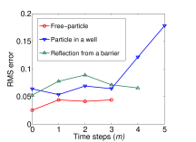
Figure 8: RMS error as a function of time-steps for the three potentials discussed in the text.

References

- Moore et al. (1965) G. E. Moore et al., “Cramming more components onto integrated circuits,” (1965).
- Feynman (1982) R. P. Feynman, International journal of theoretical physics 21, 467 (1982).
- Shory (1995) P. W. Shory, arXiv preprint quant-ph/9508027 (1995).
- Buluta and Nori (2009) I. Buluta and F. Nori, Science 326, 108 (2009).
- Lloyd (1996) S. Lloyd, Science 273, 1073 (1996).
- Lloyd and Braunstein (1999) S. Lloyd and S. L. Braunstein, Phys. Rev. Lett. 82, 1784 (1999).
- Farhi and Gutmann (1998) E. Farhi and S. Gutmann, Physical Review A 58, 915 (1998).
- Havel et al. (2002) T. Havel, D. Cory, S. Lloyd, N. Boulant, E. Fortunato, M. Pravia, G. Teklemariam, Y. Weinstein, A. Bhattacharyya, and J. Hou, American Journal of Physics 70, 345 (2002).
- Negrevergne et al. (2005) C. Negrevergne, R. Somma, G. Ortiz, E. Knill, and R. Laflamme, Physical Review A 71, 032344 (2005).
- Leibfried et al. (2002) D. Leibfried, B. DeMarco, V. Meyer, M. Rowe, A. Ben-Kish, J. Britton, W. M. Itano, B. Jelenković, C. Langer, T. Rosenband, and D. J. Wineland, Phys. Rev. Lett. 89, 247901 (2002).
- Zhang et al. (2005) J. Zhang, G. L. Long, W. Zhang, Z. Deng, W. Liu, and Z. Lu, Phys. Rev. A 72, 012331 (2005).
- Lanyon et al. (2010) B. P. Lanyon, J. D. Whitfield, G. Gillett, M. E. Goggin, M. P. Almeida, I. Kassal, J. D. Biamonte, M. Mohseni, B. J. Powell, M. Barbieri, et al., Nature Chemistry 2, 106 (2010).
- Du et al. (2010) J. Du, N. Xu, X. Peng, P. Wang, S. Wu, and D. Lu, Phys. Rev. Lett. 104, 030502 (2010).
- Soares-Pinto et al. (2011) D. O. Soares-Pinto, J. Teles, A. M. Souza, E. R. Deazevedo, R. S. Sarthour, T. J. Bonagamba, M. S. Reis, and I. S. Oliveira, International Journal of Quantum Information 09, 1047 (2011).
- Rao et al. (2013) K. Rao, A. S. De, U. Sen, H. Katiyar, T. S. Mahesh, and A. Kumar, arXiv preprint arXiv:1301.1834 (2013).
- Suter et al. (2010) D. Suter et al., Frontiers of physics in China 5, 1 (2010).
- Benenti and Strini (2008) G. Benenti and G. Strini, American Journal of Physics 76, 657 (2008).
- Nielsen and Chuang (2010) M. A. Nielsen and I. L. Chuang, Quantum computation and quantum information (Cambridge university press, 2010).
- Boashash (2003) B. Boashash, Time frequency analysis (Access Online via Elsevier, 2003).
- Wiesner (1996) S. Wiesner, arXiv preprint quant-ph/9603028 110 (1996).
- Zalka (1998) C. Zalka, Fortschritte der Physik 46, 877 (1998).
- Strini (2002) G. Strini, Fortschritte der Physik 50, 171 (2002).
- Cavanagh et al. (1995) J. Cavanagh, W. J. Fairbrother, A. G. Palmer III, and N. J. Skelton, Protein NMR spectroscopy: principles and practice (Academic Press, 1995).
- Cory et al. (1998) D. Cory, M. Price, and T. Havel, Physica D 120, 82 (1998).
- Knill et al. (1998) E. Knill, I. Chuang, and R. Laflamme, Physical Review A 57, 3348 (1998).
- Mahesh and Kumar (2001) T. S. Mahesh and A. Kumar, Physical Review A 64, 12307 (2001).
- Knill et al. (2000) E. Knill, R. Laflamme, R. Martinez, and C.-H. Tseng, Nature 404, 368 (2000).
- Roy and Mahesh (2010) S. S. Roy and T. S. Mahesh, Physical Review. A 82 (2010).
- Fung (2001) B. Fung, Physical Review A 63, 022304 (2001).