Properties of Magnetic Neutral Line Gradients and Formation of Filaments

Abstract

We investigate gradient of magnetic field across neutral lines (NLs), and compare their properties for NLs with and without the chromospheric filaments. Our results show that there is a range of preferred magnetic field gradients where the filament formation is enhanced. On the other hand, a horizontal gradient of magnetic field across a NL alone does not appear to be a single factor that determines if a filament will form (or not) in a given location.

1 Introduction

Chromospheric filaments (prominences at the limb) are one of the major features characterizing the solar activity in low solar atmosphere (chromosphere and low corona). Filament eruptions are at the core of many solar-terrestrial effects or Space Weather. The filaments are formed along magnetic polarity inversion lines, but only a minority of these neutral lines (NLs) has filaments above them. Several studies were made trying to find the necessary conditions for filament formation, but still there is no clear understanding of this [Mackay et al. (2010)]. It was found by previous studies that filaments form only in filament channels (for review, see Gaizauskas1998), which overlay NLs. Some studies have indicated that the convergence of magnetic flux leading to either flux cancellation or reconnection is required for filament formation (see Mackay2008; Martin1998; Martin1990, and references therein). Recently, Martin2012 suggested that formation of filament and filament channels is part of development of large-scale chiral systems. In our present study, we concentrate only on properties of neutral lines, and do not consider other aspects of filament formation (such as, for example, role of helicity).

Gaizauskas2001 have shown that one important condition for the formation of a filament channel is a strong horizontal component of magnetic field aligned with the magnetic neutral line. Thus, one can ask if the properties (and evolution) of magnetic NLs could be sufficient to identify potential location of filament formation? Indeed, several studies (e.g., Maksimov1995; Nagabhushana1990) have suggested that the gradient of magnetic field transverse to the neutral line may play a significant role in filament formation. According to Demoulin1998 one of the necessary conditions for the filament formation is a low gradient of magnetic field transverse to NL.

Here we conduct a statistical study of horizontal gradients of magnetic field across neutral lines, and investigate how these properties differ for NLs with filaments and without them. We also investigate whether the properties of neutral lines change with solar cycle, and whatever this change can be the cause of variation in filaments length and total number with the solar cycle.

2 Data and Data Analysissec:data

We employ daily H$\alpha$ full-disk images from Mauna Loa Solar Observatory (MLSO) and SOHO/MDI (Michelson Doppler Imager) synoptic maps for 1997-2010 years. For our main H$\alpha$ data set, we included daily full-disk images corresponding to two complete Carrington rotations (CRs) per year with a time separation between selected CRs about five months. However, due to lack of data, only one rotation was taken for the years 1997, 2003, and 2010; and for year 2000, we selected three (non-consecutive) solar rotations. In addition to MDI synoptic maps (for same Carrington rotations as our H$\alpha$ data), we also use the Synoptic Optical Long-term Investigations of the Sun (SOLIS, Bala2011) synoptic maps and the full-disk magnetograms taken at Ca II 854.2 nm chromospheric line to study properties of the chromospheric neutral lines.

Because of the statistical nature of our study, we automated the identification of filaments (using H$\alpha$ full-disk images) and neutral lines (using MDI synoptic maps). Several studies were made in developing filament automatic detection (e.g., Shih2003; Qu2005; Scholl2008; Joshi2010). Most of them have an extensive algorithm of filament detection from an image taken in a single wavelength or use multiple images taken in different wavelengths. In our algorithm, we used both H$\alpha$ daily full-disk images and magnetograms. This allowed us to significantly simplify the process of filament detection by comparing the location of potential filaments (dark features initially found on H$\alpha$ images) with underlying magnetic field. This approach also helped to reduce (computer) processing time.

The criterion for filament identification is an intensity threshold which is defined as an average intensity over the full-disk image minus two standard deviations of the average. All pixels satisfying the above criterion (but excluding pixels near the limb) are considered as potential filaments. The final selection takes into account existence of NL inside the filament contour. Magnetic neutral lines were identified on synoptic maps after smoothing them by 50 x 50 pixels running window.

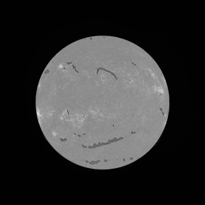
Figure 1.: H${\alpha}$ full-disk image with filament contours as identified by our automated procedure. fig1

Figure 1 shows an example of a H$\alpha$ full-disk image with filament contours found by our automated procedure. It is clear that our procedure successfully identifies all major filaments. Small clumps of filament material could be missed especially in locations near the solar limb. For example, while the procedure identifies one clump of filament material near the North polar region (near the top of solar disk in Figure 1), it misses several other clumps in the same location. As an additional test, for a few selected solar rotations, we compared our filament identification with the data from the BASS2000 Solar Survey Database (bass2000.obspm.fr). Figure 2 demonstrates a very good agreement between filaments from BASS2000 data base (green), and those identified by our method (red).

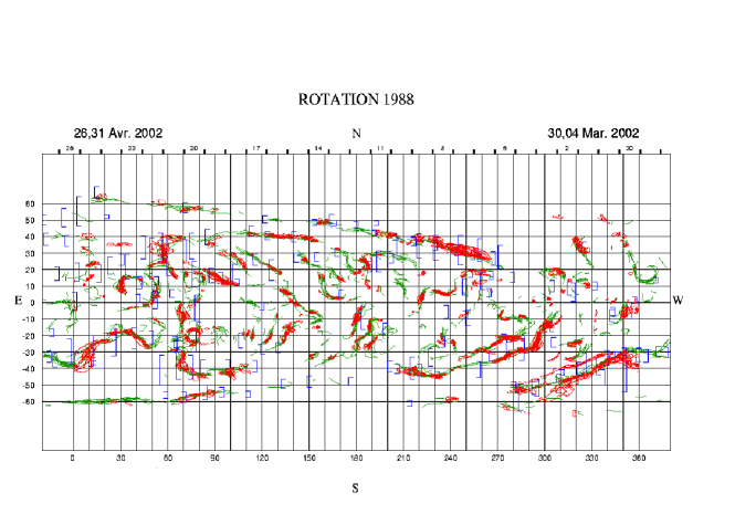
Figure 2.: Filaments from BASS2000 Solar Survey Database (green) and our identification method (red). fig2

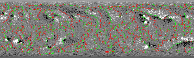
Figure 3.: Example of MDI synoptic map for the Carrington Rotation 1932 with neutral lines. Green color is used for type A lines (inside one bipolar region) and red is for type B lines (between two bipolar regions). Black/white corresponds to negative/positive polarities. fig3

Figure 3 is an MDI synoptic map with neutral lines drawn in different colors. The colors are used to indicate the type of NL: green is for the lines between magnetic polarities inside one active region, and red is for the lines separating polarities of two different active regions. For the reasons of automation, the determination of a type of NL (inter/intra- active region) is based on the polarity of fields to the West and East of the neutral line. If the orientation of these two polarities followed the Hale polarity rule, we called the neutral line as intra-active region. Otherwise, it was classified as inter-region NL. Inevitably, this approach mis-identifies non-Hale polarity active regions. But the fraction of such regions is very minor, and thus, the effect on overall statistics is insignificant.

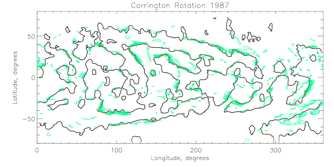
Figure 4.: Example of neutral lines (black) with filament contours (green). Parts of neutral lines that have filaments are marked by red color. fig4

Figure 4 provides example of neutral lines associated with the chromospheric filaments as identified by our procedure. The portions of neutral lines with filaments are marked by red color.

Although we analyze only two solar rotations per year, our data set of filaments is representative of a complete data. For example, a latitudinal distribution of filaments in our data set exhibits well-known latitudinal drift (e.g., Li2010). During the rising phase of solar activity, the filaments distribution (in our set) shows a clear preference for high latitudes, and as the cycle progresses, more filaments are found at lower latitudes following the equatorward drift similar to sunspot’s butterfly diagram.

3 Displacement of filaments with respect to neutral lines

While the chromospheric filaments are located above the magnetic neutral lines, it is not uncommon to see a displacement between the location of a NL (as measured in the photosphere) and the filament body (as observed in H$\alpha$) in full-disk images. One can contribute such a displacement to the fact that filaments are the features located at certain heights above the photosphere and to their projection to the image plane.

However, our analysis suggests that this displacement could not be explained by a simple projection effect alone. To further explore this displacement, we analyzed a number of filaments observed near the central meridian. High-latitude filaments ($|$lat$|{\geq}$ 60 degrees) were excluded from this analysis. We also compared the change in filament-NL displacements for selected filaments near the East and West limbs. The displacements between the filament body and the neutral line were present in different locations independent of closeness to the limb or the central meridian. In some cases, only a part of a filament was displaced relative to closest neutral line, while the rest of the filament was perfectly aligned with NL. Figure 5 (left panel) shows one such an example.

Since the filaments could be located at a certain height above the photosphere, one could argue that their location should correlate better with the neutral lines of the chromospheric fields (which are formed higher in the atmosphere). Contrary to this expectation, some filaments show a larger displacement relative to closest chromospheric neutral line as compared with the photospheric NL (compare left and right panels in Figure 5). Thus, the displacement of filament location (as seeing in image plane of the photospheric and chromospheric magnetograms) is clearly not due to a projection effect alone.

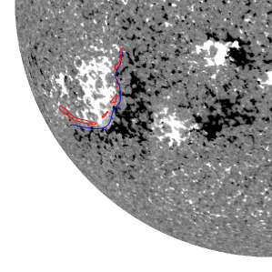
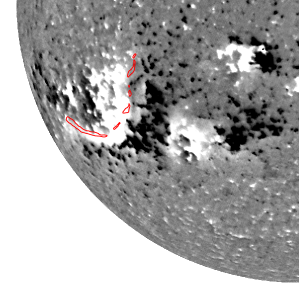
Figure 5.: Example of filament displacement with respect to neutral line on photospheric (left) and chromospheric (right) magnetogram from VSM on SOLIS. Blue line represents neutral line, red contour - a filament. Black/white corresponds to negative/positive polarities. fig5

One possible explanation for the displacements described above is that the ”neutral lines” are not lines but planes separating opposite polarities. These ”polarity inversion planes” are not always vertical, but they could be inclined depending on flux systems they separate. One can visualize this as a ribbon (perhaps, a current sheet) “waving” around the isolated coronal flux systems. The intersection of this polarity inversion plane with the photosphere corresponds to the photospheric neutral line, and the filament can form within this plane higher up. If this interpretation is correct, the displacement between the photospheric NL and filament body would be an interplay between the location (height) of filament within the polarity inversion plane and the tilt of the plane relative to solar surface. The idea that (some) chromospheric filaments are sheet-like structures is not new. We simply use it to demonstrate that a broadly held belief that the filaments are located above magnetic neutral lines should be taken with a clear understanding that in image plane that location of filament bodies and the neutral lines could be displaced from each other, and not only due to elevation of filament above the photosphere, but also because of its height geometry.

In some cases of relatively weak (and fragmented) magnetic fields, the exact location of the photospheric neutral line is very uncertain. In some of these cases, a continuous photospheric neutral line may not even exist underneath of a filament. For example, filament segment in the low-right corner of Figure 6 overlies patch of negative polarity; there appears no clear neutral line (of photospheric field) that can be associated with this filament segment.

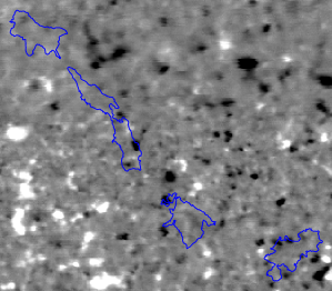
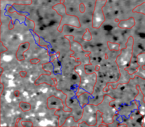
Figure 6.: Example of a filament contour (blue) displayed on magnetogram. Red color is used for neutral lines. Black/white corresponds to negative/positive polarities. fig6

The inconsistencies between the location of filaments and the photospheric/ chromospheric neutral lines described in this section may indicate that the filament location is governed by the coronal magnetic fields rather than the photospheric or even the chromospheric fields.

As a rule, we find a better agreement between the neutral lines and filament positions when we use synoptic maps. We speculate that since these maps are based on an averaged magnetic field, they may better represent the large-scale magnetic domains. Even though for filament identification we employ daily full-disk images, we do average filament positions over several days, and thus, any projection effects are minimized.

Based on the results of the analysis presented in this Section, for our study of magnetic properties of NLs we chose to use the synoptic magnetograms.

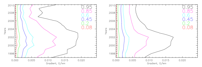
Figure 7.: Temporal variation of gradient distribution. Left - for NLs with filaments, right - for lines without filaments. Colored contours correspond to fraction of gradients below a certain value. For instance, for year 1997 95% of all NL without filaments have gradients below 0.0088 G km^-1 (right panel). fig7

4 Role of gradient of magnetic fieldsec:results

First, we investigate gradients of magnetic field across the neutral line and their variation with level of solar activity. Figure 7 shows temporal variation of gradient distribution for NLs with filaments (left panel) and without them (right panel). The gradients were computed at uniformly spaced intervals along magnetic neutral lines. Then, each segment was identified either as having a filament or not based on proximity of filament material to this part of neutral line. We did not attempt any averaging of field gradients for individual filaments. Different colors are used to indicate the fraction of NLs with a specific property. For example, contour labeled 0.95 means that 95% of the NLs have gradients less or equal of gradient shown as abscissa on Figure 7. For instance, for the year 1997, 95% of NLs with filaments (Figure 7, left) have gradients ${\leq}$ 0.011 G km^-1, while 95 % of NLs without filaments (Figure 7, right) have gradients ${\leq}$ 0.0088 G km^-1.

At the first glance, the distributions of gradients across NLs with and without filaments are very similar. However, neutral lines with filaments exhibit systematically stronger gradients as compared with NLs without filaments (compare Figure 7 left and right panels). Filaments are observed above the NLs with gradients ranging from 6.6 $\times$ 10^-5 G km^-1 to 0.11 G km^-1. Only a small fraction of filaments are formed above the NLs with gradients outside that range. A fraction of the neutral lines with gradients smaller than about 0.001 G km^-1 is about 20% for NLs with or without filaments, and it does not seem to vary with solar activity cycle. A fraction of neutral lines with gradients higher than 0.005 G km^-1 shows a strong variation with solar activity cycle. By its amplitude, NLs with and without filaments show comparable change between solar minimum and maximum: for NLs with filaments, 95% level decreases from about 0.019 G km^-1 (year 2002) to about 0.007 G km^-1 (year 2009), while for NLs without filaments it changes from 0.017 G km^-1 (year 2002) to 0.006 G km^-1 (year 2009). On the other hand, the changes for NLs with filaments occur over a longer period of time (i.e., peak corresponding to 95% level on Figure 7 left panel is much ”broader” as compared with Figure 7, right panel). In 2002, about 50% (between 0.95 and 0.45 contours in Figure 7) NLs with filaments fall within 0.019-0.0035 G km^-1. In the same year, 35% of all filaments (between 0.95 and 0.45 contours in Figure 7) formed above NLs within 0.019-0.005 G km^-1 range of gradients. In comparison, 50% of NLs without filaments fell within 0.017-0.0025 G km^-1, and 35% of NLs (without filaments) were in 0.017-0.004 G km^-1 range. In 2004, 50% (0.95-0.45 levels in Figure 7) of filaments developed above NLs with 0.0155-0.0022 G km^-1 magnetic field gradients, while 50% NLs without filaments fall within 0.0095-0.0018 G km^-1 range of gradients. During periods of low sunspot activity (i.e., 2007-2009), neutral lines with and without filaments have similar range of gradients (e.g., in 2007, 85% of neutral lines with and without filaments were below about 0.005 G km^-1 (c.f., Figure 7 left and right panels).

Thus, our data show a clear tendency for NLs with filaments to have stronger magnetic gradients during the rising and declining phases and the maximum of solar cycle, as compared with NLs without filaments. Although filaments are formed above the NLs with a wide range of gradients, there appears to be a preferred range of gradients where filaments are observed more often. This preferred range covers gradients from about 0.0025 to 0.019 G km^-1. Less than 20% of filaments were formed at gradients below about 0.001 G km^-1, and less than about 5% of filaments have developed above NLs with 0.0019 G km^-1 (at solar maximum). On the other hand, having ”preferred” horizontal gradient does not guarantee the filament formation there; large fraction of NLs which exhibit similar gradients remains empty of filament material. Furthermore, on average, only a small fraction of neutral lines is associated with filaments. This fraction varies from about 2% at solar minimum to 15% at solar maximum (Figure 8).

Figure 8.: Fraction of NL total length occupied by filaments as a function of time. Solid line shows measurements from selected Carrington rotations, and the dashed line represents 5-point central moving average. fig8

Next, we investigate the properties of magnetic field gradients for different types of filaments. One of the earliest classification schemes (e.g., Tang1987) segregates filaments on two categories based on the nature of the NL above which the filament lies. If filament overlays a neutral line separating two polarities forming an active region, it is classified as a ‘bipolar region filament’, or type A. When filament is formed above a NL that separates two different active regions, it is called a ‘between bipolar region filament’, or type B. To automate the categorization of NLs, we assigned their type based on magnetic polarity orientation and the Hale polarity rule (i.e., if the (leading-following) polarity orientation for a given NL agrees with the Hale-Nicholson polarity rule, this NL and filament above it were classified as type A). Otherwise, the NL (and a filament) were classified as type B. Example of such classification is shown in Figure 2. Green color is used for type A lines and red color – for type B. Although this simplified approach allows an automatic identification of the type of NLs and filaments, it has a limitation of mis-identifying NLs and filaments associated with non-Hale polarity regions. Likely, only a small fraction (about a few percent) of all active regions disobeys the Hale-Nicholson polarity rule.

Two types of NLs (and filaments) do not appear to show any significant difference in properties of magnetic gradients. We did find, however, a slight preference for filaments to form in between active regions (type B) at a rising phase of solar cycle, while type A filaments (inside active region) were more abundant at the declining phase of cycle.

Lastly, we expanded our investigation to the neutral lines derived from the chromospheric magnetic fields observed by Vector Spectromagnetograph (VSM) on SOLIS. We applied the same technique as for the photospheric magnetograms. The results are very similar to those derived from the photospheric fields with respect to the pattern of gradients described above.

5 Discussionsec:summary

We studied the properties of horizontal gradients across neutral lines depending on presence or absence of filaments above them. We found a preferred range of NL gradients where filaments are observed relatively more frequently. Still only about 18% of neutral lines within that ”preferred range” of gradients have filaments above them. Thus, a mere fact that a horizontal gradient across magnetic neutral line falls within a ”preferred” range does not guarantee that a filament will form in that location. One cannot exclude, however, that together with other factors these gradient properties could play a role in creating overall conditions for filament formation. Thus, for example, several studies suggested that convergence of magnetic field may be required for the filament formation (e.g., Martin1990; Martin1998; Mackay2008). Another factor that could play important role in filament formation is the rate of canceling magnetic features that were hypothesized to supply the material to filaments [Martin (1998), Litvinenko and Martin (1999)]. Due to spatial and temporal limitation of the data set used in this study, we did not investigate the role of these other factors in filament formation.

The gradients for neutral lines with filaments show similar variations with the solar cycle as do the neutral lines without filaments (i.e., an increase in fraction of stronger gradients during the maximum of solar activity). However, this change in properties of gradients for NLs with filaments is enhanced during the rising and declining phases of cycle, while the properties of NLs without filaments are more narrowly defined to a maximum of solar cycle. During these periods (of rising and declining phases of solar cycle), a larger fraction of NLs within preferred range of gradients is occupied by filaments.

Although we did not find a strong preponderance of filament formation on the properties of magnetic gradients of neutral lines, our data do suggest that there is a range of magnetic gradients preferred for filament formation. A cyclic increase in fraction of neutral lines (with these preferred gradients) may provide enhancement in favorable conditions for more filament formation during solar maximum. However, there is a need for an additional mechanism(s) that takes advantage of the above favorable conditions to create more filaments. Such additional condition could be the amount of material in the corona available for filament formation. One can speculate that during solar maximum, overall conditions in the photosphere and chromosphere (e.g., enhanced network fields, larger number of small-scale reconnection events etc.) may result in a significantly larger amount of material supplied to the corona. In combination with the increased fraction of NLs with stronger gradients, having more material in the corona may create more opportunities for condensation of this material to form the chromospheric filaments.

Finally, the noted displacement of filaments (with respect to the photospheric neutral lines) and the lack of a strong correlation between the gradient properties of NLs and filament formation may suggest that filament formation is governed by properties of coronal magnetic fields rather than the photospheric or chromospheric magnetic fields. In itself, this may fit better with the model in which the excess of material in the corona combined with changes in properties of NLs at solar cycle maximum is the prime reason for a solar cycle variation in chromospheric filaments. At the present, no such model exists.

Acknowledgements

The authors acknowledge funding from NASA’s NNH09AL04I inter agency transfer and NSF grant AGS-0837915. This work utilizes SOLIS data obtained by the NSO Integrated Synoptic Program (NISP), managed by the National Solar Observatory, which is operated by the Association of Universities for Research in Astronomy (AURA), Inc. under a cooperative agreement with the National Science Foundation. SOHO is a project of international cooperation between ESA and NASA. National Solar Observatory (NSO) is operated by the Association of Universities for Research in Astronomy, AURA Inc under cooperative agreement with the National Science Foundation (NSF).

References

- Balasubramaniam and Pevtsov (2011) Balasubramaniam, K.S. and Pevtsov, A.: 2011, Ground-based Synoptic Instrumentation for Solar Observations, Society of Photo-Optical Instrumentation Engineers (SPIE) CS-8148, 814809.
- Démoulin (1998) Démoulin, P.: 1998, Magnetic Fields in Filaments, in A.S.P. Conf. Series, Vol. 150, IAU Colloq. 167: New Perspectives on Solar Prominences, eds. David Webb, David Rust, Brigitte Schmieder (San Francisco: ASP), 78.
- Gaizauskas (1998) Gaizauskas, V.: 1998, “Filament Channels: Essential Ingredients for Filament Formation”, in A.S.P. Conf. Series, Vol. 150, IAU Colloq. 167: New Perspectives on Solar Prominences, eds. David Webb, David Rust, Brigitte Schmieder (San Francisco: ASP), 257.
- Gaizauskas, Mackay, and Harvey (2001) Gaizauskas, V., Mackay, D. H., Harvey, K. L.: 2001, Astrophys. J. 558, 888.
- Joshi, Srivastava, and Mathew (2010) Joshi, A. D., Srivastava, N., Mathew, S. K.: 2010, Solar Phys. 262, 425.
- Li (2010) Li, K. J.: 2010, Monthly Notices of the Royal Astronomical Society 405, 1040.
- Litvinenko and Martin (1999) Litvinenko, Y. E., Martin S. F.: 1999, Solar Phys. 190, 45.
- Mackay, Gaizauskas and Yeates (2008) Mackay, D. H., Gaizauskas, V., Yeates, A. R.: 2008, Solar Phys. 248, 51.
- Mackay et al. (2010) Mackay, D. H., Karpen, J. T., Ballester, J. L., Schmieder, B., Aulanier, G.: 2010, Space Sci. Rew., 151, 333.
- Maksimov and Prokopiev (1995) Maksimov, V. P. Prokopiev, A. A.: 1995, Astron. Nachrichten, 316, 249.
- Martin (1990) Martin, S. F.: 1990, Lecture Notes in Physics, 363, 1.
- Martin (1998) Martin, S. F.: 1998, Solar Phys. 182, 107.
- Martin et al. (2012) Martin, S.F., Panasenco, O., Berger, M.A., Engvold, O., Lin, Y., Pevtsov, A.A., Srivastava, N.: 2012, Second ATST-EAST Meeting: Magnetic Fields from the Photosphere to the Corona. 463, 157.
- Nagabhushana and Gokhale (1990) Nagabhushana, B.S., Gokhale, M.H.: 1990, Lecture Notes in Physics, 363, 234.
- Qu et al. (2005) Qu, M., Shih, F. Y., Jing, J., Wang, H.: 2005, Solar Phys. 228, 119.
- Scholl and Habbal (2008) Scholl, I. F., Habbal, S. R.: 2008, Solar Phys. 248, 425.
- Shih and Kowalski (2003) Shih, F. Y. Kowalski, A. J.: 2003, Solar Phys. 218, 99.
- Tang (1987) Tang, F.: 1987, Solar Phys. 107, 233.