Semantic Context Forests for Learning-Based Knee Cartilage Segmentation in 3D MR Images

Abstract

The automatic segmentation of human knee cartilage from 3D MR images is a useful yet challenging task due to the thin sheet structure of the cartilage with diffuse boundaries and inhomogeneous intensities. In this paper, we present an iterative multi-class learning method to segment the femoral, tibial and patellar cartilage simultaneously, which effectively exploits the spatial contextual constraints between bone and cartilage, and also between different cartilages. First, based on the fact that the cartilage grows in only certain area of the corresponding bone surface, we extract the distance features of not only to the surface of the bone, but more informatively, to the densely registered anatomical landmarks on the bone surface. Second, we introduce a set of iterative discriminative classifiers that at each iteration, probability comparison features are constructed from the class confidence maps derived by previously learned classifiers. These features automatically embed the semantic context information between different cartilages of interest. Validated on a total of 176 volumes from the Osteoarthritis Initiative (OAI) dataset, the proposed approach demonstrates high robustness and accuracy of segmentation in comparison with existing state-of-the-art MR cartilage segmentation methods.

1 Introduction

The quantitative analysis of knee cartilage is advantageous for the study of cartilage morphology and physiology. In particular, it is an important prerequisite for the clinical assessment and surgical planning of the cartilage diseases, such as knee osteoarthritis which is characterized as the cartilage deterioration and a prevalent cause of disability among elderly population. As the leading imaging modality used for articular cartilage quantification [1], magnetic resonance (MR) imaging provides direct and noninvasive visualization of the whole knee joint including the soft cartilage tissues (Fig. 1c). However, automatic segmentation of the cartilage tissues from MR images, which is required for accurate and reproducible quantitative cartilage measures, still remains an open problem because of the inhomogeneity, small size, low tissue contrast, and shape irregularity of the cartilage.

An earlier endeavor on this problem is Folkesson et al.’s voxel classification approach [2], which runs an approximate $k$NN classifier on voxel intensity and absolute position based features. However, due to the overlap of intensity distribution between cartilage and other tissues such as menisci and muscles, as well as the variability of the cartilage locations from scan to scan, the performance of this method is limited. More recently, Vincent et al. have developed a knee joint segmentation approach based on active appearance model (AAM), which captures the statistics of both object shape and image cues. Though promising results are reported in [3], the search for the initial model pose parameter can be very time consuming even if a coarse to fine searching strategy is used.

Given the strong spatial relation between the cartilages and bones in the knee joint, most proposed cartilage segmentation methods are based on a framework that each bone is segmented first in the knee joint [4, 5, 6], which is usually easier than direct cartilage segmentation because the bones are much larger in size with more regular shapes. Fripp et al. segment the bones based on 3D active shape model (ASM) incorporating the cartilage thickness statistics, and the outer cartilage boundary is then determined by examining the intensity profile along the normal to the bone surface, while being constrained by the cartilage thickness model [4]. In Yin’s work [5], the volume of interest containing the bones and cartilages is first detected using a learning-based approach, then the bones and cartilages are jointly segmented by solving an optimal multi-surface detection problem via multi-column graph cuts [7]. Lee et al. employ a constrained branch-and-mincut method with shape priors to obtain the bone surface, and then segment the cartilage with MRF optimization based on local shape and appearance information [6]. In spite of the differences, these approaches all require classification of bone surface voxels into bone cartilage interface (BCI) and non-BCI, which is an important intermediate step to determine the search space or impose prior constraint for cartilage segmentation. Therefore, any classification error of BCI will probably propagate to the final cartilage segmentation result.

In this paper, we present a fully automatic learning-based voxel classification method for cartilage segmentation. It also requires pre-segmentation of corresponding bones in the knee joint. However, the new approach does not rely on explicit classification of BCI. Instead, we construct distance features from each voxel to a large number of anatomical landmarks on the surface of the bones to capture the spatial relation between the cartilages and bones. By removing the intermediate step of BCI extraction, the whole framework is simplified and classification error propagation can be avoided.

Besides the connection between the cartilages and bones, strong spatial relation also exists among different cartilages which is more often overlooked in earlier approaches. For example, the femoral cartilage is always above the tibial cartilage and two cartilages touch each other in the region where two bones slide over each other during joint movements. To utilize this constraint, we introduce the iterative discriminative classification that at each iteration, the multi-class probability maps obtained by previous classifiers are used to extract semantic context features. In particular, we compare the probabilities at positions with random shift and compute the difference. These features, which we name as the random shift probability difference (RSPD) features, are more computationally efficient and more flexible for different range of context compared to the calculation of probability statistics at fixed relative positions [8, 9].

2 Review of Bone Segmentation

In this work, we employ a learning-based bone segmentation approach which has shown the efficiency and effectiveness in different medical image segmentation problems [10, 11]. We represent the shape of a bone by a closed triangle mesh $\mathcal{M}$. Given a number of training volumes with manual bone annotations, we use the coherent point drift algorithm (CPD) [12] to find anatomical correspondences of the mesh points and thereof construct the statistical shape models with mean shape $\overline{\mathcal{M}}$ [13]. As shown in Fig. 1a, the whole bone segmentation framework comprises three steps.

1. Pose Estimation: For a volume $\mathcal{V}$, the bone is first localized by searching for the (sub-)optimal pose parameters $(\hat{t},\hat{r},\hat{s})$, i.e., the translation, rotation and anisotropic scaling, using the marginal space learning (MSL) [11]:

   $$(\hat{t},\hat{r},\hat{s})\approx(\arg\max_{t}P(t|\mathcal{V}),\arg\max_{r}P(r|\mathcal{V},\hat{t}),\arg\max_{s}P(s|\mathcal{V},\hat{t},\hat{r})),\vspace{-3mm}$$ (1)

   and the shape is initialized by linearly transforming the mean shape $\overline{\mathcal{M}}$.

2. Model Deformation: At this stage, the shape is repeatedly deformed to fit the boundary and projected to the variation subspace until convergence.

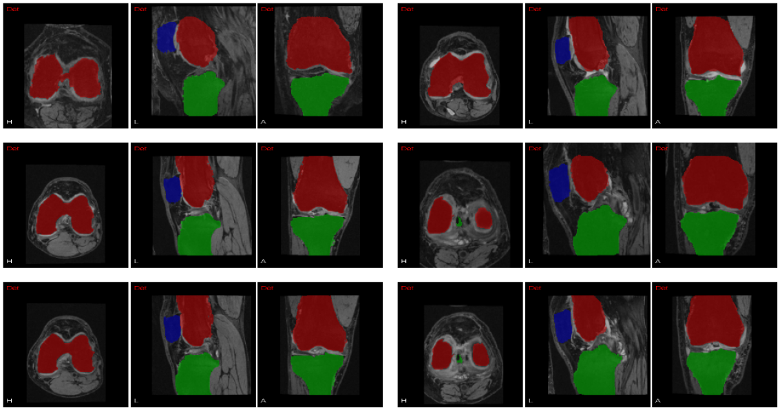
Figure 4: Example bone segmentations. Each case has three views, from left to right: transversal plane, sagittal plane, coronal plane. Red: femur; green: tibia; blue: patella.

3. Boundary Refinement: To further improve the segmentation accuracy, we use the random walks algorithm [14] to refine the bone boundary (see Table 1 and Fig. 4 for results) and employ the CPD algorithm to obtain anatomically equivalent landmarks on the refined bone surface.

3 Cartilage Classification

Given all three knee bones being segmented, we first extract a band of interest within a maximum distance threshold from each of the bone surface, and only classify voxels in the band of interest to simplify the training and testing by removing irrelevant negative voxels.

3.1 Feature Extraction

For each voxel with spatial coordinate $\mathbf{x}$, we construct a number of base features which can be categorized into three subsets.

Intensity Features include the voxel intensity and its gradient magnitude, respectively: $f_{1}(\mathbf{x})=I(\mathbf{x})$, $f_{2}(\mathbf{x})=||\nabla I(\mathbf{x})||$.

Distance Features measure the signed Euclidean distances from each voxel to different knee bone boundaries: $f_{3}(\mathbf{x})=d_{F}(\mathbf{x})$, $f_{4}(\mathbf{x})=d_{T}(\mathbf{x})$, $f_{5}(\mathbf{x})=d_{P}(\mathbf{x})$, where $d_{F}$ is the signed distance to the femur, $d_{T}$ to tibia, and $d_{P}$ to patella. Then we have their linear combinations:

$$f_{6/7}(\mathbf{x})=d_{F}(\mathbf{x})\pm d_{T}(\mathbf{x}),\qquad\qquad f_{8/9}(\mathbf{x})=d_{F}(\mathbf{x})\pm d_{P}(\mathbf{x}).\vspace{-2mm}$$ (2)

These features are useful because the sum features $f_{6}$ and $f_{8}$ measure whether voxel $\mathbf{x}$ locates within the narrow space between two bones, and the difference features $f_{7}$ and $f_{9}$ measure which bone it is closer to. Fig. 3b shows how $f_{6}$ and $f_{7}$ in addition to intensity feature $f_{1}$ separate tibial cartilage from femoral and patellar cartilages.

Given the prior knowledge that the cartilage can only grow in certain area on the bone surface, it is useful for the cartilage segmentation to not only know how close the voxel is to the bone surface, but also where it is anatomically. Therefore we define the distance features to the densely registered landmarks on the bone surface as described in Section 2: $f_{10}(\mathbf{x,\zeta})=||\mathbf{x}-\mathbf{z}_{\zeta}||$, where $\mathbf{z}_{\zeta}$ is the spatial coordinate of the $\zeta$th landmark of all bone mesh points. $\zeta$ is randomly generated in training due to the great number of mesh points available (Fig. 3a).

	Femur DSC (%)	Tibia DSC (%)	Patella DSC (%)
Before RW	$92.37\pm 1.58$	$94.64\pm 1.18$	$92.07\pm 1.47$
After RW	$94.86\pm 1.85$	$95.96\pm 1.64$	$94.31\pm 2.15$

Table 1: The Dice similarity coefficient (DSC) of bone segmentation results before and after random walks (3-fold cross validation on 176 OAI volumes).

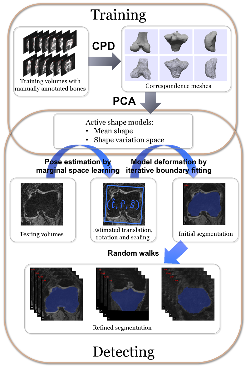
(a)

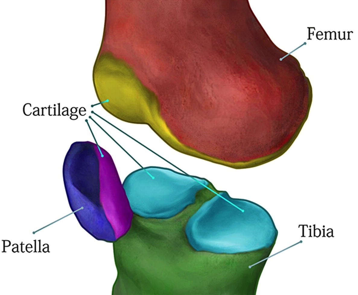
(b)

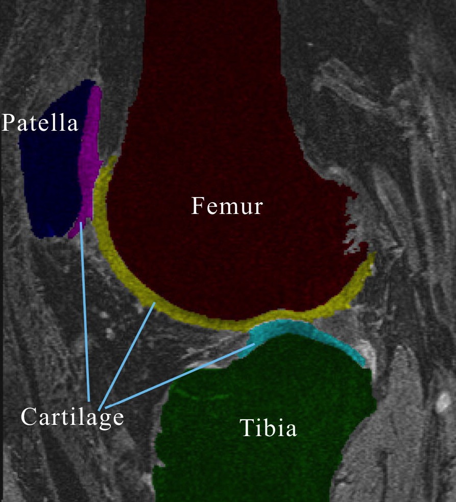
(c)

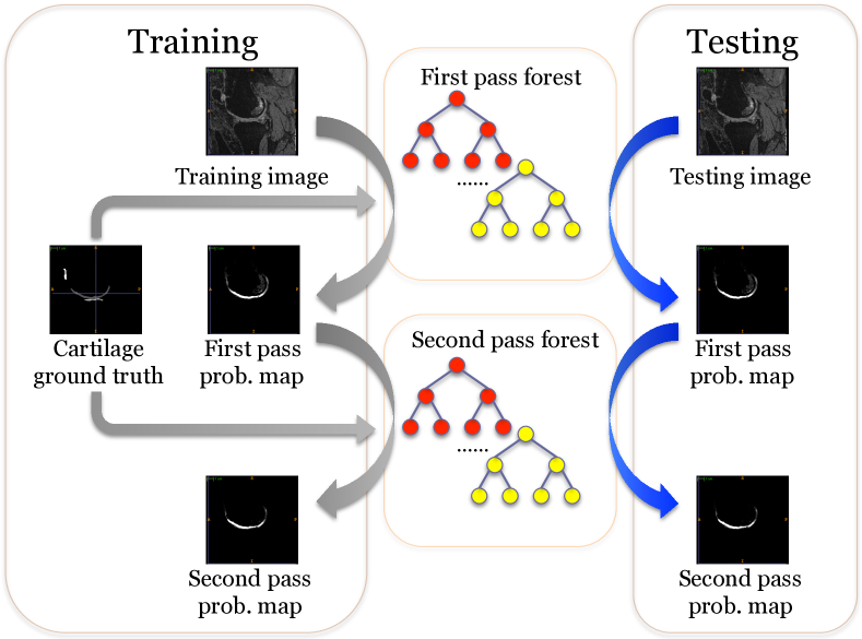
(d)

Figure 1: (a) The bone segmentation framework. (b) 3D anatomy of knee joint. (c) Example of a 2D MR slice [6]. (d) The semantic context forests diagram.

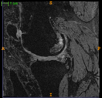
(a)

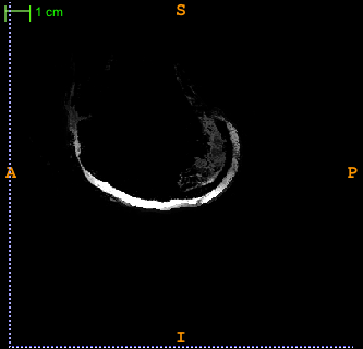
(b)

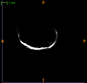
(c)

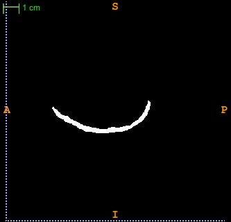
(d)

Figure 2: Probability maps of femoral cartilage by semantic context forests. (a) Original image. (b) Prob. map of the 1st pass. (c) Prob. map of the 2nd pass. (d) Ground truth.

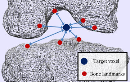
(a)

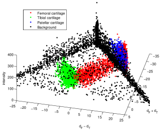
(b)

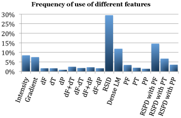
(c)

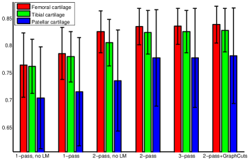
(d)

Figure 3: (a) Distances to densely registered bone landmarks encode anatomical position of a voxel. (b) Feature scatter plot: intensity and distance features separate tibial cartilage from femoral and patellar cartilages. (c) Frequency of each feature selected by the classifier in the 2nd pass. (d) A comparison of segmentation performance (DSC): 1-pass/2-pass forests without using distance to landmark (LM) features; 1-pass/2-pass/3-pass forests using distance to landmark features; 2-pass forests with graph cuts optimization (3-fold cross validation).

Context Features compare the intensity of the current voxel $\mathbf{x}$ and another voxel $\mathbf{x}+\mathbf{u}$ with random offset $\mathbf{u}$: $f_{11}(\mathbf{x,u})=I(\mathbf{x+u})-I(\mathbf{x})$, where $\mathbf{u}$ is a random offset vector. This subset of features, named as random shift intensity difference (RSID) features in this paper, capture the context information in different ranges by randomly generating a large number of different values of $\mathbf{u}$ from a uniform distribution in training. They were earlier used to solve pose classification [15] and keypoint recognition [16] problems.

3.2 Iterative Semantic Context Forests

In this paper, we present a multi-pass iterative classification method to automatically exploit the semantic context for multiple object segmentation problems. In each pass, the generated probability maps will be used to extract the context embedded features to enhance the classification performance of the next pass. Fig. 1d shows a 2-pass iterative classification framework with the random forests [15, 16, 17, 18, 19, 20] selected as the base classifier for each pass. However, the method can be extended to more iterations with the use of other discriminative classifiers.

Semantic Context Features

After each pass of the classification, the probability maps are generated and used to extract semantic context features as defined below: $f_{12}(\mathbf{x})=P_{F}(\mathbf{x})$, $f_{13}(\mathbf{x})=P_{T}(\mathbf{x})$, $f_{14}(\mathbf{x})=P_{P}(\mathbf{x})$, where $P_{F}$, $P_{T}$ and $P_{P}$ stand for the femoral, tibia and patellar cartilage probability map, respectively. In the same fashion as the RSID features, we compare the probability response of two voxels with random shift:

$$f_{15/16/17}(\mathbf{x},\mathbf{u}) = P_{F/T/P}(\mathbf{x+u})-P_{F/T/P}(\mathbf{x}),\vspace{-2mm}$$ (3)

which is called random shift probability difference features (RSPD). RSPD provides semantic context information because the probability map values are directly associated with anatomical labels, rather than original intensity volume.

In Fig. 2, it can be observed that the probability map of the second pass classification is significantly enhanced with much less noisy responses, compared with the first pass.

3.3 Post-processing by Graph Cuts Optimization

After the classification, we finally use the probabilities of being the background and the three cartilages to construct the energy functions and perform multi-label graph cuts [21] to refine the segmentation with smoothness constraints.

The graph cuts algorithm assigns a label $l(\mathbf{x})$ to each voxel $\mathbf{x}$, such that the energy below is minimized:

$$E(L)=\sum\limits_{\{\mathbf{x,y}\}\in\mathcal{N}}V_{\mathbf{x,y}}(l(\mathbf{x}),l(\mathbf{y}))+\sum\limits_{\mathbf{x}}D_{\mathbf{x}}(l(\mathbf{x})),$$ (4)

where $L$ is the global label configuration, $\mathcal{N}$ is the neighborhood system, $V_{\mathbf{x,y}}(\cdot)$ is the smoothness energy, and $D_{\mathbf{x}}(\cdot)$ is the data energy. We define

$$D_{\mathbf{x}}(l(\mathbf{x})) = -\lambda\ln P_{l(\mathbf{x})}(\mathbf{x}),$$ (5)

$$V_{\mathbf{x,y}}(l(\mathbf{x}),l(\mathbf{y})) = \delta_{l(\mathbf{x})\neq l(\mathbf{y})}e^{\frac{(I(\mathbf{x})-I(\mathbf{y}))^{2}}{2\sigma^{2}}}.$$ (6)

$\delta_{l(\mathbf{x})\neq l(\mathbf{y})}$ takes value 1 when $l(\mathbf{x})$ and $l(\mathbf{y})$ are different labels, and takes value 0 when $l(\mathbf{x})=l(\mathbf{y})$. $P_{l(\mathbf{x})}(\mathbf{x})$ takes the value $P_{F}(\mathbf{x})$, $P_{T}(\mathbf{x})$, $P_{P}(\mathbf{x})$ or $1-P_{F}(\mathbf{x})-P_{T}(\mathbf{x})-P_{P}(\mathbf{x})$, depending on the label $l(\mathbf{x})$. $\lambda$ and $\sigma$ are two parameters. $\lambda$ specifies the weight of data energy versus smoothness energy, while $\sigma$ is associated with the image noise [22].

4 Experimental Results

4.1 Dataset and Experiment Settings

The dataset we use in our work is the publicly available Osteoarthritis Initiative (OAI) dataset, which contains both 3D MR images and ground truth cartilage annotations, referred to as “kMRI segmentations (iMorphics)”. The sagittal 3D 3T (Tesla) DESS (dual echo steady state) WE (water-excitation) MR images in OAI have high-resolution, good delineation of articular cartilage, fast acquisition time and high SNR. Our dataset consists of 176 volumes from 88 subjects, and belongs to the Progression subcohort, where all subjects show symptoms of OA. Each subject has two volumes scanned in different years. The size of each image volume is $384\times 384\times 160$ voxels, and the voxel size is $0.365\times 0.365\times 0.7\,\mathrm{mm^{3}}$.

For the validation, we divide the OAI dataset to three equally-sized subsets: $D_{1}$, $D_{2}$ and $D_{3}$, and perform a three-fold validation. The two volumes from the same subject are always placed in the same subset. For each randomized decision tree, we set the depth of the tree to 18, and train 60 trees in each pass. During training, the number of candidates at each non-leaf node is set to 1000. The dice similarity coefficient (DSC) is used to measure the performance of our method since it is commonly reported in previous literature [2, 4, 5, 6, 23].

4.2 Results

First, we compare the frequency of different features that is selected by the classifiers. As shown in Fig. 3c, RSID, RSPD and the distance to dense landmarks are very informative features to embed spatial constraints.

Then we compare the segmentation performance with and without the use of the distance features to the anatomical dense landmarks, and also the results with different number of classification iterations. The results in Fig. 3d demonstrate the effectiveness of the distance features to dense landmarks and iterative classification with semantic context forests. In particular, 2-pass random forests achieve significant performance improvement, whereas the gain seems quite negligible by adding more passes.

Finally, the quantitative results (2-pass classification) are listed in Table 2 together with the numbers reported in the earlier literature. Because the datasets used are different by all these approaches, the numbers in the table are only for reference. Note that only our experiments are based on a relatively large dataset. As shown in the table, we achieved high performance with regard to the femoral and tibial cartilage, whereas the DSC of patellar cartilage is notably lower than the other two cartilages. This is partly because the size of patellar cartilage is much smaller than femoral and tibial cartilage, so that the same amount of segmentation error will result in lower DSC. Besides, some patellar cartilage annotations in the dataset do not appear very consistent with others. Example segmentation results are shown in Fig. 5.

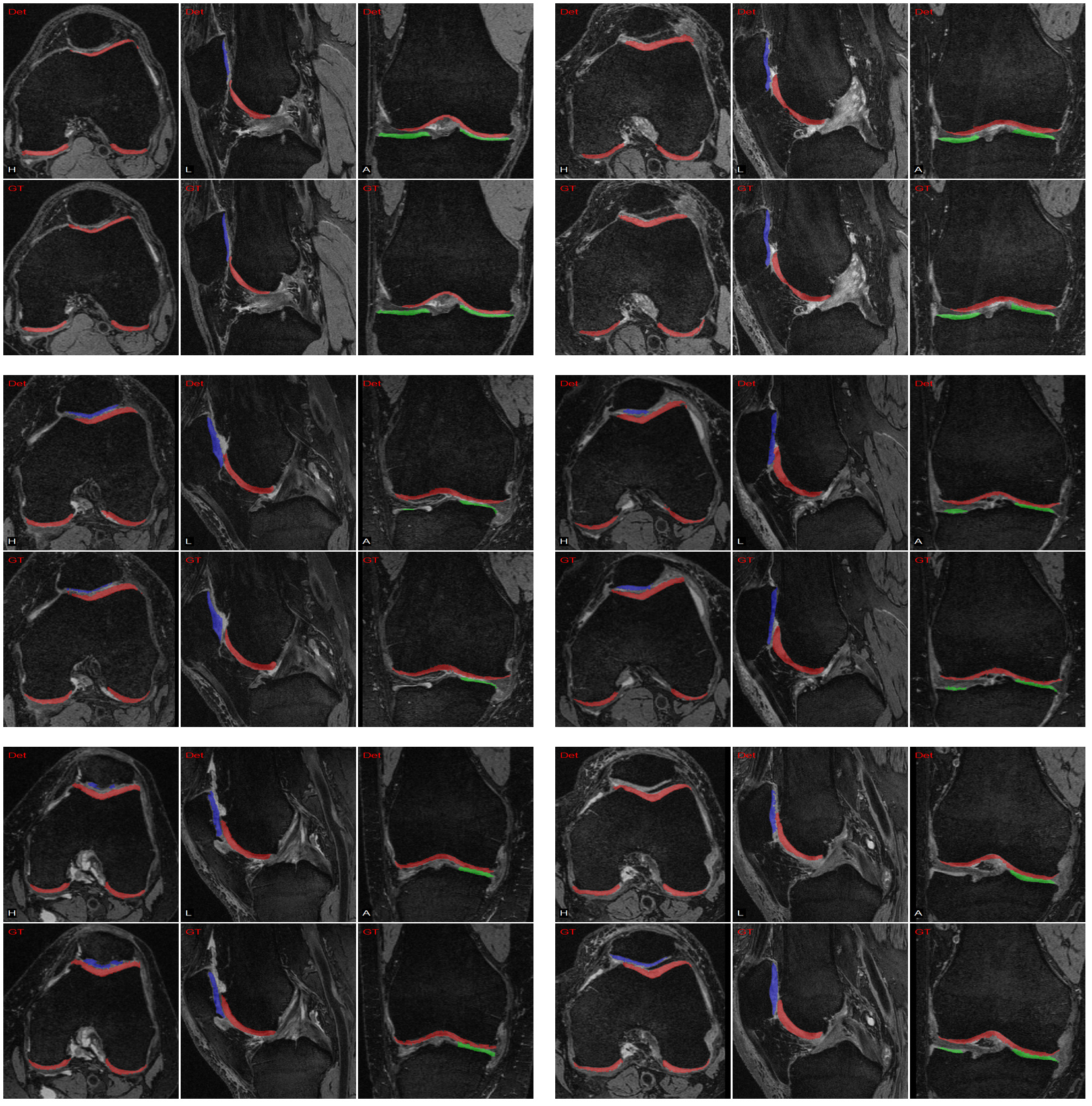
Figure 5: Examples cartilage segmentations compared with ground truth. Each case has six images: segmentation results in upper row, ground truth in lower row. Red: femoral cartilage; green: tibial cartilage; blue: patellar cartilage.

5 Conclusion

We have presented a new approach to segment the three knee cartilages in 3-D MR images, which effectively exploits the semantic context information in the knee joint. By using the distance features to the bone surface as well as to the dense anatomical landmarks on the bone surface, the spatial constraints between cartilages and bones are incorporated without the need of explicit extraction of the bone cartilage interface. Furthermore, the use of multi-pass iterative classification with semantic context forests provides more spatial constraints between different cartilages to further improve the segmentation. The experiment validation shows the effectiveness of this method. Ongoing work include the joint bone-and-cartilage voxel classification in the iterative classification framework.

		Fem. Cart. DSC		Tib. Cart. DSC		Pat. Cart. DSC
Author	Dataset	Mean	Std.	Mean	Std.	Mean	Std.
Shan [23]	18 SPGR images	78.2%	5.2%	82.6%	3.8%	–	–
Folkesson [2]	139 Esaote C-Span images	77%	8.0%	81%	6.0%	–	–
Fripp [4]	20 FS SPGR images	84.8%	7.6%	82.6%	8.3%	83.3%	13.5%
Lee [6]	10 images in OAI	82.5%	–	80.8%	–	82.1%	–
Yin [5]	60 images in OAI	84%	4%	80%	4%	80%	4%
	OAI, $D_{1}$ subset (58 images)	85.47%	3.10%	84.96%	3.82%	78.56%	9.38%
Proposed	OAI, $D_{2}$ subset (58 images)	85.20%	3.65%	83.52%	4.08%	80.79%	7.40%
method	OAI, $D_{3}$ subset (60 images)	84.22%	3.05%	82.74%	3.84%	78.12%	9.63%
	OAI, overall (176 images)	84.96%	3.30%	83.74%	4.00%	79.16%	8.88%

Table 2: Performance of our method compared with other state-of-the-art cartilage segmentation methods: mean DSC and standard deviation.

References

- [1] Graichen, H., Eisenhart-Rothe, R., Vogl, T., Englmeier, K.H., Eckstein, F.: Quantitative assessment of cartilage status in osteoarthritis by quantitative magnetic resonance imaging. Arthritis Rheumatism (2004)
- [2] Folkesson, J., Dam, E., Olsen, O., Pettersen, P., Christiansen, C.: Segmenting articular cartilage automatically using a voxel classification approach. IEEE Trans. Med. Imag. 26(1) (Jan. 2007) 106–115
- [3] Vincent, G., Wolstenholme, C., Scott, I., Bowes, M.: Fully automatic segmentation of the knee joint using active appearance models. In: Medical Image Analysis for the Clinic: A Grand Challenge. (2010)
- [4] Fripp, J., Crozier, S., Warfield, S., Ourselin, S.: Automatic segmentation and quantitative analysis of the articular cartilages from magnetic resonance images of the knee. IEEE Trans. Med. Imag. 29(1) (Jan. 2010) 55–64
- [5] Yin, Y., Zhang, X., Williams, R., Wu, X., Anderson, D., Sonka, M.: Logismos – layered optimal graph image segmentation of multiple objects and surfaces: Cartilage segmentation in the knee joint. IEEE Trans. Med. Imag. 29(12) (Dec. 2010) 2023–2037
- [6] Lee, S., Park, S.H., Shim, H., Yun, I.D., Lee, S.U.: Optimization of local shape and appearance probabilities for segmentation of knee cartilage in 3-d mr images. CVIU 115(12) (Dec. 2011) 1710–1720
- [7] Li, K., Wu, X., Chen, D., Sonka, M.: Optimal surface segmentation in volumetric images–a graph-theoretic approach. IEEE Trans. PAMI 28(1) (Jan. 2006) 119–134
- [8] Tu, Z., Bai, X.: Auto-context and its application to high-level vision tasks and 3d brain image segmentation. IEEE Trans. PAMI (Oct. 2010) 1744–1757
- [9] Montillo, A., Shotton, J., Winn, J., Iglesias, J., Metaxas, D., Criminisi, A.: Entangled decision forests and their application for semantic segmentation of ct images. In: IPMI. (2011) 184–196
- [10] Ling, H., Zheng, Y., Georgescu, B., Zhou, S.K., Suehling, M.: Hierarchical learning-based automatic liver segmentation. In: CVPR. (2008)
- [11] Zheng, Y., Barbu, A., Georgescu, M., Scheuring, M., Comaniciu, D.: Four-chamber heart modeling and automatic segmentation for 3D cardiac CT volumes using marginal space learning and steerable features. IEEE Trans. Med. Imag. 27(11) (2008) 1668–1681
- [12] Myronenko, A., Song, X.: Point set registration: Coherent point drift. IEEE Trans. PAMI 32(12) (Dec. 2010) 2262–2275
- [13] Cootes, T., Taylor, C., Cooper, D., Graham, J.: Active shape models–their training and application. CVIU 61(1) (1995) 38–59
- [14] Grady, L.: Random walks for image segmentation. IEEE Trans. PAMI 28(11) (Nov. 2006) 1768–1783
- [15] Shotton, J., Fitzgibbon, A., Cook, M., Sharp, T., Finocchio, M., Moore, R., Kipman, A., Blake, A.: Real-time human pose recognition in parts from single depth images. In: CVPR. (Jun. 2011) 1297–1304
- [16] Lepetit, V., Lagger, P., Fua, P.: Randomized trees for real-time keypoint recognition. In: CVPR. Volume 2. (Jun. 2005) 775–781 vol. 2
- [17] Quinlan, J.R.: Induction of decision trees. Machine learning 1(1) (1986) 81–106
- [18] Breiman, L.: Random forests. Machine learning 45(1) (2001) 5–32
- [19] Wang, Q., Ou, Y., Julius, A.A., Boyer, K.L., Kim, M.J.: Tracking Tetrahymena Pyriformis Cells using Decision Trees. In: ICPR. (Nov. 2012)
- [20] Zikic, D., Glocker, B., Konukoglu, E., Shotton, J., Criminisi, A., Ye, D., Demiralp, C., Thomas, O., Das, T., Jena, R., et al.: Context-sensitive classification forests for segmentation of brain tumor tissues, MICCAI (2012)
- [21] Boykov, Y., Veksler, O., Zabih, R.: Fast approximate energy minimization via graph cuts. IEEE Trans. PAMI 23(11) (Nov. 2001) 1222–1239
- [22] Boykov, Y., Funka-Lea, G.: Graph cuts and efficient n-d image segmentation. Int. J. Comput. Vis. 70(2) (Nov. 2006) 109–131
- [23] Shan, L., Charles, C., Niethammer, M.: Automatic atlas-based three-label cartilage segmentation from mr knee images. In: 2012 IEEE Workshop on Mathematical Methods in Biomedical Image Analysis. (Jan. 2012) 241–246