Quantum-classical comparison: arrival times and statistics

Abstract

Classical and quantum scattering of a non-Gaussian wave packet by a rectangular barrier is studied in terms of arrival times to a given detector location. A classical wave equation, proposed by N. Rosen [Am. J. Phys. 32 (1964) 377], is used to study the corresponding classical dynamics. Mean arrival times are then computed and compared for different values of initial wave packet parameters and barrier width. The agreement is improved in the large mass limit as one expects. A short comment on the possibility of generalization of Rosen’s proposal to a two-body system is given. Differences in distributions of particles obeying different statistics are studied by considering a system composed of two free particles.

I Introduction

The classical limit of quantum mechanics is continuously an interesting research topic Ho_book_1993_1 ; Ba-book-1998 ; Home-book-1997 . It is often considered that $\hbar\rightarrow 0$ gives the classical limit. Other limits that are very often used are large quantum numbers (correspondence principle), short de Broglie wavelengths and large masses. It has been argued that the limit $\hbar\rightarrow 0$ is conceptually and mathematically problematic. In addition, different possible limiting procedures that can be used in a given problem are mathematically inequivalent Ho_book_1993_1 . Very recently, a dividing line between quantum and classical trajectories in the continuous measurement process has been proposed leading to the so-called Bohmian time constant antonio2013 .

It is well known that the wave function $\psi$ provides statistical knowledge of the state of a system. The classical analog of this system corresponds to an ensemble of particles following deterministic trajectories. Thus, comparison of classical and quantum mechanics should be meaningful provided that their statistical predictions for the dynamical evolutions of the same given initial ensemble is used, apart from some version of the correspondence principle. Quantum mechanics is formulated in Hilbert space while classical statistical mechanics is formulated in phase space. Thus, the corresponding evolution equations are the Schrödinger and Liouville equations, respectively. According to Feynman in his dynamical theory of the Josephson effect FeLeSa-book-1965 , classical and quantum mechanics may be embedded in the same Hamiltonian formulation by using complex canonical coordinates St-RMP-1966 ; He-PRD-1985 . Based on Heslot’s work He-PRD-1985 , a theory of quantum-classical hybrid dynamics has been proposed Elz-PRA-2012 , which concerns the direct coupling of classical and quantum mechanical degrees of freedom. Application of this proposal to entanglement dynamics and mirror-induced decoherence has been studied FrLaEl-arxiv-2014 ; LaFrEl-arxiv-2014 .

For a given system, the initial phase space distribution of an ensemble is not uniquely defined. The simplest choice is to take a product of the position and momentum distributions. Based on this scheme, the quantum-classical correspondence of an arrival time distribution has been considered in terms of a non-minimum-uncertainty-product Gaussian wave packet (known as a squeezed state) which evolves in the presence of a linear potential HoPaBa-JPA-2009 ; Ri-JPA-2013 ; HoPaBa-JPA-2013 . In particular, it was shown by Riahi Ri-JPA-2013 that, if the compared initial distribution functions are Gaussian with identical statistical properties, the quantum and the classical mean arrival times are the same under the influence of at most quadratic potentials. Moreover, for potentials of the form $V(x)=Ax^{2}+Bx+C$, the Liouville equation for the classical phase space distribution function coincides with the evolution equation for the Wigner function Ba-book-1998 . So, if both functions coincide initially, they will coincide all the time in such a potential. Home et al. HoPaBa-JPA-2009 have taken the initial classical phase space distribution as the product of the position and the momentum distributions, and this is the point which has been criticized by Riahi. This author, in contrast, considers the initial phase space distribution function to be the Wigner function that is evaluated using the given initial wave function. In their reply, Home et al. state that it is not desirable to use any quantum input to fix the initial conditions for classical calculations when one considers classical limit of quantum mechanics.

An alternative route which has been less used in literature, it is that initially proposed by Rosen Ro-AJP-1964 . He argues that, in the large mass limit, the Schrödinger equation should be replaced by another Schrödinger-like equation, known as classical wave equation, which is equivalent to the classical continuity and Hamilton-Jacobi equations. He, by speculation, conjectured that transition from quantum domain to the classical one takes place for masses of the order of $m_{0}=2.18\times 10^{-5}$g or larger.

This classical wave equation contains a non-linear term in $\psi$ which in general prevents superposition of different states unless these states do not overlap or can be expressed as a multiplication of each other. Thus, instead of superposition, pure states are combined to produce mixed states Ro-AJP-1965 . For instance, in the scattering of a wave packet by a barrier, if the the energy is less than the barrier height, the solutions of the classical wave equation, that is, the incident and reflected functions describe independent motions, without no interference effects. On the contrary, in the corresponding quantum problem, the quantum pure state remains pure and there is no classical limit Ho_book_1993_1 .

In this work, our aim is to examine the quantum-classical correspondence by analyzing the dynamics of a wave packet with different barrier parameters and masses in terms of mean arrival times. The detector location is situated well behind the barrier to prevent some overlapping. We would like to provide a criterion for the magnitude of mass for which the classical wave equation of Rosen should be used instead of the Schrödinger equation. Then we consider a two-body system and discuss about the possibility of generalization of Rosen’s classical wave equation. Although particles are non-interacting, due to the symmetry of the total wave function spatial correlations exist. By deriving one-body distributions, we study differences between fermions and bosons.

II Scattering of a wave packet by a rectangular barrier and arrival times

Consider a beam of incident particles from the left by a rectangular potential barrier defined as $V(x)=V_{0}\Theta(x)\Theta(a-x)$, where $\Theta(x)$ is the step function and $a$ is the corresponding width. An ideal detector placed at $x=X~{}\gg~{}a$, very far from the barrier, can detect transmitted particles at a given time. The initial wave function is assumed to be of the form

$$\psi_{0}(x) = R_{0}(x)e^{ip_{0}x/\hbar}~{},$$ (1)

in the region $x<0$, which is a plane wave modulated by the variable amplitude $R_{0}(x)$ and with initial momentum $p_{0}$. The corresponding initial, classical phase space distribution function is

$$D_{0}(x,p)=\left\{\begin{array}[]{ll}|R_{0}(x)|^{2}\delta(p-p_{0}),&\mbox{$x<0$}\\ 0,&\mbox{$x>0$.}\end{array}\right.$$ (2)

This initial wave function describes classically a set of particles having the same momentum $p_{0}$. Quantum mechanically a momentum distribution is usually assumed. When the incident energy is greater than the barrier height, that is, $E_{0}=p_{0}^{2}/2m>V_{0}$, classically, all particles of mass $m$ ultimately cross the barrier and arrive at the detector location, $X$. However, quantum mechanically, the particles can also be reflected by the barrier. Due to the fact the detector is located very far from the barrier, then it suffices to consider only the transmitted part of the initial wave packet.

II.1 Quantum treatment

Once an incident particle coming from the left of the barrier has passed completely through it, the transmitted part of the wave packet is given by CoDiLa_book_1977

$$\psi_{T}(x,t)=\frac{1}{\sqrt{2\pi}}\int_{0}^{\infty}dk~{}e^{i(kx-E_{k}t/\hbar)}T(k)\phi(k)~{},$$ (3)

where $E_{k}=\hbar^{2}k^{2}/2m$, $\phi(k)$ being the Fourier transform of the initial wave function and

$$T(k)=\frac{4kqe^{i(q-k)a}}{(k+q)^{2}-(k-q)^{2}e^{2iaq}}~{},$$ (4)

is the transmission probability amplitude for monochromatic incidence with $q=\sqrt{2m(E_{k}-V_{0})/\hbar^{2}}$.

If the width of the momentum distribution is sufficiently narrow, the wave packet does not suffer an important distortion or reshaping Wi-PR-2006 because of approximate constancy of the transmission coefficient over the range of the corresponding integral

$$\psi_{T}(x,t)=\frac{1}{\sqrt{2\pi}}|T(k_{0})|\int_{0}^{\infty}dke^{i[kx-E_{k}t/\hbar+\eta(k)]}\phi(k)~{},$$ (5)

where $\eta(k)$ is the phase of $T(k)$ and $k_{0}$ corresponds to the maximum of $\phi(k)$.

II.2 Classical treatment

Rosen Ro-AJP-1964 discussed and proposed a nonlinear equation in the configuration space of the form

$$i\hbar\frac{\partial\psi}{\partial t}=\left(-\frac{\hbar^{2}}{2m}\nabla^{2}+V+\frac{\hbar^{2}}{2m}\frac{\nabla^{2}|\psi|}{|\psi|}\right)\psi~{},$$ (6)

instead of the Schrödinger equation for the case of large mass particles, very often known as the classical Schrödinger equation. If the wave function is written in polar form as $\psi(x,t)=R(x,t)e^{iS(x,t)/\hbar}$, and is substituted in that equation one readily obtains

$$\frac{\partial S}{\partial t}+\frac{(\nabla S)^{2}}{2m}+V = 0~{},$$ (7)

$$\frac{\partial\rho}{\partial t}+\nabla\cdot{\bf{j}} = 0,$$ (8)

which are the classical Hamilton-Jacobi and continuity equations, respectively. Here $\rho=R^{2}$ represents the probability density of an ensemble of trajectories associated with the same S-function, ${\bf{j}}=\frac{\hbar}{m}\Im(\psi^{*}\nabla\psi)=R^{2}\frac{\nabla S}{m}$ the probability current density and $S$ the classical action. The real functions $R$ and $S$ are primary and the classical wave function $\psi$ is deduced from them, i.e., it has ”a purely descriptive or mathematical significance” Ho_book_1993_2 . From Eqs. (7) and (8), one easily reaches the continuity of $S$ and ${\bf{j}}\cdot\hat{\bf{n}}$ at a surface where the potential energy changes discontinuously; $\hat{\bf{n}}$ being the normal to the surface Ro-AJP-1965 .

When $E_{0}=p_{0}^{2}/2m>V_{0}$, the solution of the classical wave equation with initial condition (1) is given by

$$\psi_{C}(x,t)=\left\{\begin{array}[]{lll}R_{0}\left(x-\frac{p_{0}t}{m}\right)e^{i[p_{0}x-E_{0}t]/\hbar}&\mbox{$x<0$,}\\ \sqrt{\frac{p_{0}}{p^{\prime}_{0}}}R_{0}\left[\frac{p_{0}}{p^{\prime}_{0}}\left(x-\frac{p^{\prime}_{0}t}{m}\right)\right]e^{i(p^{\prime}_{0}x-E_{0}t)/\hbar}&\mbox{$0<x<a$ ,}\\ R_{0}\left[x-\frac{p_{0}t}{m}+a\left(\frac{p_{0}}{p^{\prime}_{0}}-1\right)\right]e^{i[p_{0}x-E_{0}t+(p^{\prime}_{0}-p_{0})a]/\hbar}&\mbox{$a<x$ .}\end{array}\right.$$ (9)

where $p^{\prime}_{0}=\sqrt{2m(E_{0}-V_{0})}$ and the continuity of the action $S$ and current density ${\bf j}$ have been used at the boundaries $x=0$ and $x=a$. The classical action $S$ generates the classical trajectory

$$x(t)=x_{0}+u.\left\{\begin{array}[]{lll}t~{}~{}~{}~{}~{}~{}~{}~{}~{}~{}~{}~{}~{},&\mbox{$0\leq t<-mx_{0}/p_{0}$}\\ \frac{p^{\prime}_{0}}{p_{0}}t~{}~{}~{}~{}~{}~{}~{}~{}~{},&\mbox{$-mx_{0}/p_{0}\leq t<m(-x_{0}/p_{0}+a/p^{\prime}_{0})$}\\ t~{}~{}~{}~{}~{}~{}~{}~{}~{}~{}~{}~{}~{}~{},&\mbox{$m(-x_{0}/p_{0}+a/p^{\prime}_{0})\leq t$ ,}\end{array}\right.$$ (10)

where $u=p_{0}/m$ is the velocity of the particle in the free region. Thus, a classical particle arrives at the detector location $X$ at time

$$t_{C}(x_{0};X)=\frac{X-x_{0}}{u}+a\left(\frac{1}{\sqrt{u^{2}-\frac{2V_{0}}{m}}}-\frac{1}{u}\right)~{}.$$ (11)

One then readily sees that $t_{C}(x_{0};X)$ decreases with the mass and increases with the barrier width, when other parameters are kept constant.

II.3 Arrival times

In both treatments, the arrival time distribution at the detector location is given by

$$\Pi(t;X) = \frac{|j(X,t)|}{\int_{0}^{\infty}dt|j(X,t)|}~{},$$ (12)

from which the mean arrival time is calculated,

$$\tau(X) = \int_{0}^{\infty}dt~{}t~{}\Pi(t;X)~{}.$$ (13)

At this point, it should be noted that in classical mechanics the concept of arrival time is clear and meaningful. Furthermore, one can easily prove that its distribution is given by (12). On the contrary, in the standard interpretation of quantum mechanics, this concept is rather controversial and there are different proposals for its definition (see, for example, Ref. MuLe-PR-2000 for a review).

Another point that has been noticed in literature is the uniqueness of the Schrödinger probability current density. Demanding that the non-relativistic current to be the non-relativistic limit of the unique relativistic current, a unique form has been derived for the probability current density of spin-$1/2$ Ho-PRA-1999 ; and spin-$0$ and spin-$1$ particles StBaNeWe-PLA-2004 . In the case of spin-$1/2$ particles for a spin eigenstate in the absence of a magnetic field, the spin-dependent term $(\hbar/m)\Re(\psi^{*}\nabla\psi)\times\hat{{\bf{s}}}$ is added to the usual Schrödinger current. Here, $\hat{{\bf{s}}}=\chi^{\dagger}\hat{\sigma}\chi$ is the spin vector and $\hat{\sigma}$ is the Pauli matrix. Spin is a quantum-mechanical intrinsic property and does not have a classical counterpart. Spin-dependent term vanished in the limit $\hbar\rightarrow 0$ or large mass limit; and in one-dimensional motion this term does not contribute. So, we put it away in our calculations.

One can also directly obtain classical mean arrival times without computing the classical arrival time distribution by means of

$$\tau_{C}(X) = \int dx_{0}~{}t_{C}(x_{0};X)~{}[R_{0}(x_{0})]^{2}$$ (14)

$$= \frac{X-\langle x_{0}\rangle}{u}+a\left(\frac{1}{\sqrt{u^{2}-\frac{2V_{0}}{m}}}-\frac{1}{u}\right)~{}.$$

Just for completeness we mention that the corresponding fluctuation $\Delta\tau_{C}$ is given by the rms width of the classical arrival time distribution

$$\Delta\tau_{C} = \sqrt{\int dx_{0}~{}[t_{C}(x_{0};X)]^{2}~{}[R_{0}(x_{0})]^{2}-[\tau_{C}(X)]^{2}}$$ (15)

$$= \frac{\sqrt{\langle x_{0}^{2}\rangle-\langle x_{0}\rangle^{2}}}{u}\equiv\frac{\sigma_{x}}{u}~{},$$

which is independent of the detector location and barrier width.

II.4 Quantum-classical correspondence for a freely evolving Gaussian packet

Before going to the general case of scattering of a non-Gaussian packet by a rectangular barrier, it is instructive at first to consider free evolution of a Gaussian packet. It’s notable that the results of the previous section are valid here by putting $a=0$ and $V_{0}=0$. By solving Eqs. (7) and (8) one obtains

$$\rho_{C}(x,t) = \rho_{0}(x-ut)=\frac{1}{\sqrt{2\pi\sigma_{0}^{2}}}\exp{\left[-\frac{(x-x_{c}-ut)^{2}}{2\sigma_{0}^{2}}\right]}~{},$$ (16)

$$S_{C}(x,t) = p_{0}x-E_{0}t~{},$$ (17)

$$j_{C}(x,t) = u.\rho_{C}(x,t)~{},$$ (18)

for the classical quantities. $\rho_{0}(x)$ stands for the initial probability density which is taken to be a Gaussian. Quantum mechanically one has

$$\rho_{Q}(x,t) = \frac{1}{\sqrt{2\pi\sigma^{2}}}\exp{\left[-\frac{(x-x_{c}-ut)^{2}}{2\sigma^{2}}\right]}~{},$$ (19)

$$S_{Q}(x,t) = S_{C}(x,t)-\frac{\hbar}{2}\tan^{-1}\left(\frac{\hbar t}{2m\sigma_{0}^{2}}\right)+\frac{(x-x_{c}-ut)^{2}\hbar^{2}t}{8m\sigma_{0}^{2}\sigma^{2}}~{},$$ (20)

$$j_{Q}(x,t) = u\left[1+\frac{\hbar^{2}t}{4m^{2}\sigma_{0}^{2}\sigma^{2}}\left(\frac{x-x_{c}}{u}-t\right)\right].\rho_{Q}(x,t)~{},$$ (21)

where $\sigma=\sigma_{0}\sqrt{1+\left(\frac{\hbar t}{2m\sigma_{0}^{2}}\right)^{2}}$. One clearly sees that in the limit $\hbar\rightarrow 0$, or in the large mass limit quantum results approaches to the corresponding classical ones. So, in this specific example these two limits give the same result.

II.5 Quantum-classical correspondence for a non-Gaussian packet

For practical purposes, we can choose $R_{0}$ to be a non-Gaussian function such as ChHoMaMoMoSi-CQG-2012

$$R_{0}(x) = \frac{1}{(2\pi\sigma_{0}^{2})^{1/4}\sqrt{1+\frac{\alpha^{2}}{2}(1-e^{-\pi^{2}/8})}}\left[1+\alpha\sin\left(\pi\frac{x-x_{c}}{4\sigma_{0}}\right)\right]$$ (22)

$$\times \exp{\left[-\frac{(x-x_{c})^{2}}{4\sigma_{0}^{2}}\right]}~{},$$

$\alpha$ being a tunable parameter showing deviation from Gaussianity; $\sigma_{0}$ and $x_{c}$ are the Gaussian ($\alpha=0$) wave packet width and center, respectively. This center is chosen to be far from the barrier in such a way that there is no overlapping with the barrier. Our main motivation to use a non-Gaussian wave packet, apart from being a more general wave packet, comes from the fact that it is rather difficult to build exactly Gaussian wave packets in real experiments. This non-Gaussian function has already been used to study the weak equivalence principle of gravity in quantum mechanics ChHoMaMoMoSi-CQG-2012 . In appendix A, some useful information about this function is provided.

From Eq. (9), the classical wave function after passing completely through the barrier now takes the form

$$\psi_{C}(x,t) = \frac{1}{(2\pi\sigma_{0}^{2})^{1/4}\sqrt{1+\frac{\alpha^{2}}{2}(1-e^{-\pi^{2}/8})}}$$ (23)

$$\times \left[1+\alpha\sin\left(\pi\frac{(x-x_{c})-u~{}t+a\left(\frac{p^{\prime}_{0}}{p_{0}}-1\right)}{4\sigma_{0}}\right)\right]$$

$$\times \exp{\left\{ik_{0}\left[x-\frac{u}{2}t+a\left(\frac{p^{\prime}_{0}}{p_{0}}-1\right)\right]\right\}}$$

$$\times \exp{\left\{-\frac{\left[(x-x_{c})-u~{}t+a\left(\frac{p_{0}}{p^{\prime}_{0}}-1\right)\right]^{2}}{4\sigma_{0}^{2}}\right\}}~{},$$

where $k_{0}=p_{0}/\hbar$. In this case, by using Eqs. (14) and (41), one obtains an analytic relation for the mean arrival time to be

$$\tau_{C}(X) = \frac{1}{u}\left(X-x_{c}-\sigma_{0}\frac{\pi e^{3\pi^{2}/32}\alpha}{\alpha^{2}(e^{\pi^{2}/8}-1)+2e^{\pi^{2}/8}}\right)$$

$$+ a\left(\frac{1}{\sqrt{u^{2}-\frac{2V_{0}}{m}}}-1\right)~{}.$$

One sees that $\tau_{C}(X)$ is linear in $X$, $x_{c}$, $\sigma_{0}$ and $a$ but not in $\alpha$. This classical mean arrival time decreases (increases) with $\sigma_{0}$ for positive (negative) values of $\alpha$ but there is no dependence on the initial width for a Gaussian packet ($\alpha=0$). This is approximately true for a non-Gaussian wave packet with a very large $\alpha$. In the large mass limit, the classical mean arrival time reduces to $\tau_{C}=(X-\langle x_{0}\rangle)/u$ which is independent of the mass for a given value of $u$. From Eqs. (15) and (42), it is apparent that the classical fluctuation $\Delta\tau_{C}$ is independent of the mass, for a given value of $u$, and is minimum for a Gaussian wave packet. Using Eqs. (5) and (43) one readily obtains,

$$\psi_{T}(x,t) \simeq \frac{1}{\sqrt{2\pi}}\left(\frac{2\sigma_{0}^{2}}{\pi}\right)^{1/4}\frac{1}{\sqrt{1+\frac{\alpha^{2}}{2}(1-e^{-\pi^{2}/8})}}$$ (25)

$$\times \left\{f(k_{0})-i\frac{\alpha}{2}\left[f(k_{+})-f(k_{-})\right]\right\}~{},$$

where

$$f(k_{j}) = |T(k_{j})|\sqrt{\frac{\pi}{\sigma_{0}^{2}\left[1+i\frac{\hbar t}{2m\sigma_{0}^{2}}-i\frac{\eta^{\prime\prime}(k_{j})}{2\sigma_{0}^{2}}\right]}}$$ (26)

$$\times \exp{\left\{ik_{j}\left[x-\frac{\hbar k_{j}}{2m}t+\frac{\eta(k_{j})}{k_{j}}\right]\right\}}~{}$$

$$\times \exp{\left\{-\frac{[(x-x_{c})-\frac{\hbar k_{j}}{m}t+\eta^{\prime}(k_{j})]^{2}}{4\sigma_{0}^{2}\left[1+i\frac{\hbar t}{2m\sigma_{0}^{2}}-i\frac{\eta^{\prime\prime}(k_{j})}{2\sigma_{0}^{2}}\right]}\right\}}~{}.$$

$\eta^{\prime}(k_{j})$ and $\eta^{\prime\prime}(k_{j})$ are respectively the first and second derivative of $\eta(k)$ with respect to $k$ at $k_{j}$; $j=0,\pm$. We have used the fact that according to (43) the amplitude $\phi(k)$ is a superposition of three Gaussian functions with the same width $\sigma_{k}=1/2\sigma_{0}$ but with different wave numbers $k_{0}$ and $k_{\pm}=k_{0}\pm\pi/4\sigma_{0}$. It has also been assumed that $\sigma_{k}$ is sufficiently narrow. Thus, the corresponding integrals have been extended from $[0,\infty]$ to $[-\infty,\infty]$ and exponentials Taylor expanded about the corresponding kick momenta. The reduction of Eqs. (23) and (25) for a Gaussian wave packet, $\alpha=0$, shows that:

• The centers of the classical and quantum wave packets differ by an amount $a(p_{0}/p^{\prime}_{0}-1)-\eta^{\prime}(k_{0})$.

• The width of the classical wave packet is constant while the width of the quantum wave packet increases with time.

With these observations classical and quantum packets , i.e., $|\psi_{C}|^{2}$ and $|\psi_{T}|^{2}$ will coincide when

$$a\left(\frac{p_{0}}{p^{\prime}_{0}}-1\right)-\eta^{\prime}(k_{0}) \rightarrow 0~{},$$ (27)

$$\left(\frac{\hbar t}{2m\sigma_{0}^{2}}-\frac{\eta^{\prime\prime}(k_{0})}{2\sigma_{0}^{2}}\right)^{2} \rightarrow 0~{},$$ (28)

and $T(k_{0})\simeq 1$.

II.6 A two-body non-interacting system

Schrödinger equation for a N-body system in 1D reads

$$i\hbar\frac{\partial\Psi(x_{1},x_{2},\cdots,x_{N},t)}{\partial t} = \left(\sum_{i=1}^{N}\frac{-\hbar^{2}}{2m_{i}}\partial_{i}^{2}+V(x_{1},x_{2},\cdots,x_{N},t)\right)\Psi(x_{1},x_{2},\cdots,x_{N},t)~{},$$ (29)

where $\partial_{i}=\frac{\partial}{\partial x_{i}}$. Generalization of Rosen’s proposal to a N-body system is straightforward. By changing the Schrödinger equation as

$$i\hbar\frac{\partial\Psi(x_{1},x_{2},\cdots,x_{N},t)}{\partial t}=\left(\sum_{i=1}^{N}\frac{-\hbar^{2}}{2m_{i}}\frac{\partial^{2}}{\partial x_{i}^{2}}+V+\sum_{i=1}^{N}\frac{\hbar^{2}}{2m_{i}}\frac{\partial_{i}^{2}\Psi}{|\Psi|}\right)\Psi(x_{1},x_{2},\cdots,x_{N},t)$$

and writing the polar form of the wavefunction $\Psi(x_{1},x_{2},\cdots,x_{N},t)=R(x_{1},x_{2},\cdots,x_{N},t)e^{iS(x_{1},x_{2},\cdots,x_{N},t)/\hbar}$ one obtains,

$$\frac{\partial S(x_{1},x_{2},\cdots,x_{N},t)}{\partial t}+\sum_{i=1}^{N}\frac{[\partial_{i}S(x_{1},x_{2},\cdots,x_{N},t)]^{2}}{2m_{i}}+V(x_{1},x_{2},\cdots,x_{N},t) = 0~{},$$

$$\frac{\partial R^{2}(x_{1},x_{2},\cdots,x_{N},t)}{\partial t}+\sum_{i=1}^{N}\partial_{i}\left(R^{2}(x_{1},x_{2},\cdots,x_{N},t)\frac{\partial_{i}S(x_{1},x_{2},\cdots,x_{N},t)}{m_{i}}\right) = 0~{}.$$ (30)

Now consider a 1D system composed of two free identical particles. Classically, particles are distinguishable and obey classical Maxwell-Boltzmann (MB) statistics. Quantum mechanically they are indistinguishable and obey different statistics. Fermions (Bosons) obey Fermi-Dirac (Bose-Einstein) statistics for which the total wavefunction must be antisymmetric (symmetric) under the exchange of particles in the system. Since particles do not interact, one can construct solutions of the Schrödinger equation from two single-particle wavefunctions $\psi_{a}$ and $\psi_{b}$ as follows:

$$\Psi_{\mathrm{MB}}(x_{1},x_{2},t) = \psi_{a}(x_{1},t)\psi_{b}(x_{2},t)~{},$$ (31)

$$\Psi_{\pm}(x_{1},x_{2},t) = N_{\pm}[\psi_{a}(x_{1},t)\psi_{b}(x_{2},t)\pm\psi_{b}(x_{1},t)\psi_{a}(x_{2},t)]~{},$$ (32)

where upper (lower) sign stands for BE (FD) statistics. If single-particle wavefunctions $\psi_{a}(x_{1},t)$ and $\psi_{b}(x_{2},t)$ are solutions of classical one-body wave equation (6) then $\psi_{a}(x_{1},t)\psi_{b}(x_{2},t)$ and $\psi_{b}(x_{1},t)\psi_{a}(x_{2},t)$ separately satisfy eq. (II.6), but due to the non-linearity of this equation symmetrized wavefunctions $\Psi_{\pm}(x_{1},x_{2},t)$ are not solutions of classical wave equation, i.e., there is no corresponding classical wave equation for indistinguishable particles as one expects.

Due to indistinguishability of identical particles for the quantum BE and FD statistics, one-body density (density probability for observing a particle at point $x$ irrespective of the position of the other particle) is given by Zelev-book-2011

$$\rho_{1}(x,t) = \int dx_{1}dx_{2}~{}\delta(x-x_{1})~{}|\Psi(x_{1},x_{2},t)|^{2}=\frac{1}{2}\left[\int dx_{2}|\Psi(x,x_{2},t)|^{2}+\int dx_{1}|\Psi(x_{1},x,t)|^{2}\right]$$ (33)

$$= |N_{\pm}|^{2}\left(~{}|\psi_{a}(x,t)|^{2}+|\psi_{b}(x,t)|^{2}\pm 2~{}\Re\left[\langle\psi_{a}(t)|\psi_{b}(t)\rangle~{}\psi^{*}_{a}(x,t)\psi_{b}(x,t)\right]~{}\right)~{},$$

where $\langle\psi_{a}(t)|\psi_{b}(t)\rangle=\int dx~{}\psi^{*}_{a}(x,t)\psi_{b}(x,t)$. It must be noted that probability distributions for finding a particle at a point $x$ are different for two particles in the classical MB statistics,

$$\rho_{1}^{(1)}(x,t)=|\psi_{a}(x,t)|^{2}~{},~{}~{}~{}~{}~{}~{}~{}~{}~{}~{}~{}~{}~{}~{}~{}~{}~{}~{}\rho_{1}^{(2)}(x,t)=|\psi_{b}(x,t)|^{2}~{}.$$ (34)

By straightforward algebra one gets a continuity equation for one-body density,

$$\frac{\partial\rho_{1}(x,t)}{\partial t}+\frac{\partial}{\partial x}j_{1}(x,t) = 0~{},$$ (35)

where,

$$j_{1}(x,t) = \frac{\hbar}{2m}\Im\left\{\int dx_{2}\Psi^{*}(x,x_{2},t)\frac{\partial\Psi(x,x_{2},t)}{\partial x}+\int dx_{1}\Psi^{*}(x_{1},x,t)\frac{\partial\Psi(x_{1},x,t)}{\partial x}\right\}$$ (36)

$$= \frac{\hbar}{m}|N_{\pm}|^{2}\Im\left\{\psi^{*}_{a}\frac{\partial\psi_{a}}{\partial x}+\psi^{*}_{b}\frac{\partial\psi_{b}}{\partial x}\pm\langle\psi_{a}(t)|\psi_{b}(t)\rangle~{}\psi^{*}_{b}\frac{\partial\psi_{a}}{\partial x}\pm\langle\psi_{b}(t)|\psi_{a}(t)\rangle~{}\psi^{*}_{a}\frac{\partial\psi_{b}}{\partial x}\right\}~{},$$

and we have used the fact that the wavefunction becomes zero as $x\rightarrow\pm\infty$. For distinguishable particles obeying classical MB statistics one has two probability current densities for each particle,

$$j_{1}^{(1)}(x,t)=\frac{\hbar}{m}\Im\left\{\psi^{*}_{a}(x,t)\frac{\partial\psi_{a}(x,t)}{\partial x}\right\}~{},~{}~{}~{}~{}~{}~{}~{}~{}~{}~{}~{}j_{1}^{(2)}(x,t)=\frac{\hbar}{m}\Im\left\{\psi^{*}_{b}(x,t)\frac{\partial\psi_{b}(x,t)}{\partial x}\right\}~{},$$ (37)

Noting eqs. (33) and (36), one sees that as long as the single-particle wavefunctions has negligible overlap, i.e., $\langle\psi_{a}(t)|\psi_{b}(t)\rangle\simeq 0$ then there is no need for symmetrization. As a result one can ignore distinguishability of particles and thus uses MB statistics for which motions of particles are independent and everything is the same as the one-body systems which was discussed in previous sections. Thus, we will not consider such a statistics anymore.

By taking the one-particle wavefunctions as Gaussian packets,

$$\psi_{i}(x,t)=(2\pi s_{ti}^{2})^{-1/4}\exp{\left[{ik_{i}(x-u_{i}t/2)-\frac{(x-u_{i}t-x_{ci})^{2}}{4s_{ti}\sigma_{0i}}}\right]},~{}~{}~{}~{}s_{ti}=\sigma_{0i}(1+i\hbar t/2m\sigma_{0i}^{2})~{},$$ (38)

with $i={a,b}$, the overlap integral is given by,

$$\langle\psi_{a}(t)|\psi_{b}(t)\rangle = \sqrt{\frac{2\sigma_{0a}\sigma_{0b}}{\sigma_{0a}^{2}+\sigma_{0b}^{2}}}~{}\exp{\left[-\frac{4(k_{a}-k_{b})^{2}\sigma_{0a}^{2}\sigma_{0b}^{2}+(x_{ca}-x_{cb})^{2}+4i(k_{a}-k_{b})(\sigma_{0b}^{2}x_{ca}+\sigma_{0a}^{2}x_{cb})}{4(\sigma_{0a}^{2}+\sigma_{0b}^{2})}\right]}~{}.$$ (39)

It is seen that overlap integral $\langle\psi_{a}(t)|\psi_{b}(t)\rangle$ is independent of time and normalization constants are given by

$$N_{\pm} = \frac{1}{\sqrt{2}}\left\{1\pm\frac{2\sigma_{0a}\sigma_{0b}}{\sigma_{0a}^{2}+\sigma_{0b}^{2}}\exp{\left[-\frac{4(k_{a}-k_{b})^{2}\sigma_{0a}^{2}\sigma_{0b}^{2}+(x_{ca}-x_{cb})^{2}}{2(\sigma_{0a}^{2}+\sigma_{0b}^{2})}\right]}\right\}^{-1/2}~{}.$$ (40)

III Results and discussion

For the calculations, the following parameters are kept fixed: $x_{c}=-50$ $\AA$, $V_{0}=5$ eV, $u=4.52\times 10^{-3}c$ and $X=75$ $\AA$, where $c$ is the light velocity in vacuum. Mean arrival time is computed quantum mechanically and classically for different masses and barrier widths. Results are expressed by using the following units: time is given in femtosecond, length in Angstrom and mass in MeV$/$c².

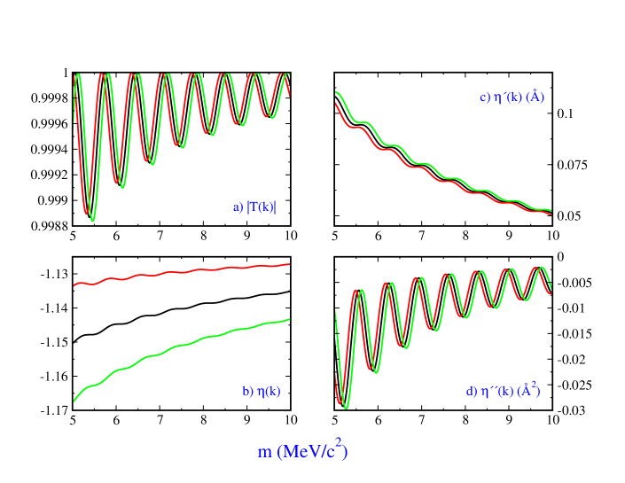
Figure 1: (Color online) a) $|T(k)|$ b) $\eta(k)$ , c) $\eta^{\prime}(k)$ and d) $\eta^{\prime\prime}(k)$ for $k=k_{0}$ (black curve), $k=k_{+}$ (red curve) and $k=k_{-}$ (green curve) versus mass for $a=2$Å.

We first present some information about the transmission probability for the wave numbers $k_{0}$ and $k=k_{\pm}$. As Eq. (25) shows, the probability density and probability current density depend on the modulus of transmission amplitude and its phase; and the first and the second derivative of the phase at $k=k_{0}$ and $k=k_{\pm}$. Figure 1 shows theses quantities as a function of the mass for a given value of barrier width. One sees all of these parameters oscillate as mass changes and oscillations become small as mass increases. At this point it is worth mentioning that the transmitted wave packet looks like the one for free propagation with minor differences in between their extrema (compare Eqs. (25) and (46)).

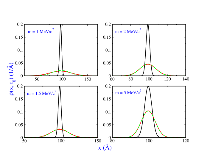
Figure 2: (Color online) Probability density for a Gaussian wave packet versus $x$ at time $t_{0}=11.07$ fs for $\sigma_{0}=2$Å and $a=8$Å; and for different values of mass. Black curve is the classical wave (23), red curve is the quantum wave computed by (25) and the green one computed by (3). One sees that red and green curves coincide as mass increases to a value $m\geq 5$ MeV$/$c².

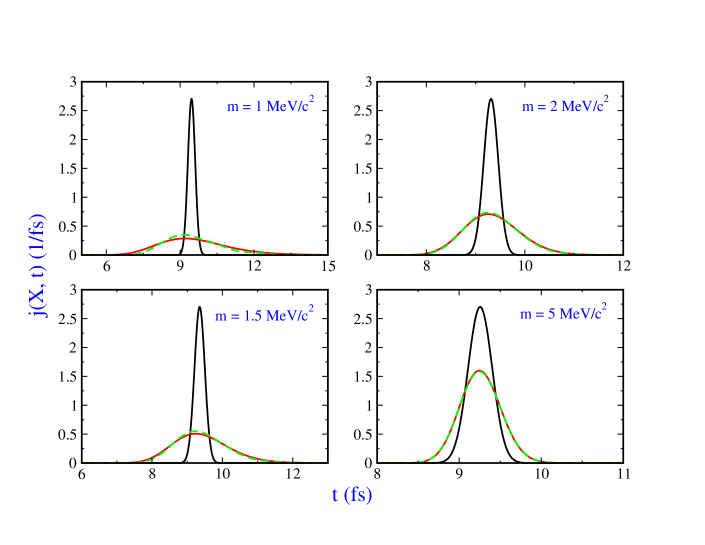
Figure 3: (Color online) Probability current density for a Gaussian wave packet versus $t$ at detector location $X=75$Å for $\sigma_{0}=2$Å and $a=8$Å; and for different values of mass. Black curve is the classical result while the red one is the quantum result computed by the wave function (25) and the green curve shows the quantum result computed by the wave function (3).

In Figures 2 and 3 we display the probability density and probability current density for a Gaussian wave packet for different values of mass. This density current is positive for all times at detector location $X$. These figures show that quantum results computed by Eqs. (25) and (3) approach as mass increases. For our working parameters, coincidence appears as $m\geq 5$MeV$/$c². Further computations show that for a given mass and barrier width $a$ these results are closer as $\sigma_{0}$ increases. Moreover, for a given mass and packet width $\sigma_{0}$, results become more similar as $a$ decreases. We have also checked that (25) and (3) give the same result as $m\geq 5$MeV$/$c², $a\leq 8$ Å and $\sigma_{0}\geq 2$Å. By choosing the parameters in this range we compute quantum mean arrival time $\tau_{Q}$ by means of the wave function (25). Finally, from Figure 4 one clearly sees that for large masses and different values of $|\alpha|$, the difference between classical and quantum mean arrival times increase. These differences decrease with mass and for a given value of $\alpha$. It is also apparent that $\tau_{C}<\tau_{Q}$, which is also a result of HoPaBa-JPA-2009 for the propagation of a non-minimum-uncertainty Gaussian wave packet in the presence of a linear gravitational field. However, this problem has been computed by a different scheme, that is, the Liouville equation instead of the classical wave equation.

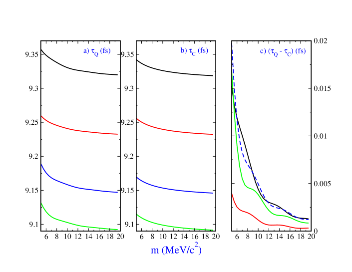
Figure 4: (Color online) a) $\tau_{Q}$, b) $\tau_{C}$ and c) $\tau_{Q}-\tau_{C}$ versus $m$ for $a=8$Å and $\sigma_{0}=2$Å; for $\alpha=-5$ (black curve), $\alpha=0$ (red curve), $\alpha=2$ (green curve) and $\alpha=5$ (blue curve).

In figure 5 we have depicted one-body densities for a two-body system composed of two identical particles. As this figure shows distributions of FD statistics are wider than that of BE ones. One-body probability current density at detector location $x_{d}=0$ shows arrival time distribution in this point. For our parameters arrival of fermions at detector location takes place sooner than bosons.

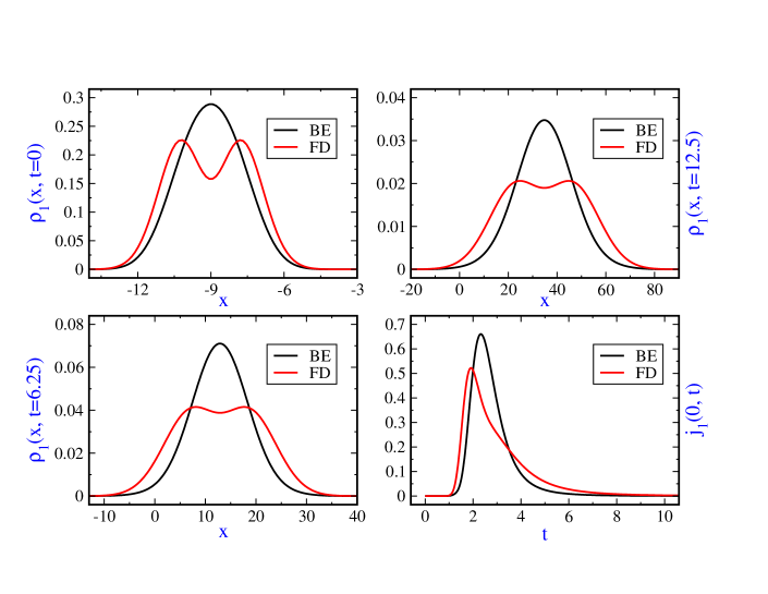
Figure 5: (Color online) one-body probability density versus space coordinate $x$ at different times and one-body probability current density versus time at detector location $x_{d}=0$. To produce this figure we have used $m=0.5$, $\hbar=1$, $k_{a}=2/\sigma_{0}$, $k_{b}=1.5/\sigma_{0}$, $x_{ca}=-10\sigma_{0}$ $x_{cb}=-8\sigma_{0}$ ,$\sigma_{0a}=\sigma_{0b}=\sigma_{0}$ and $\sigma_{0}=1$.

Summarizing, in this work, quantum and classical correspondence are studied based on the evolution of a non-Gaussian wave packet in configuration space under the presence of a rectangular potential barrier. Mean arrival times, at a given detector location, are analyzed classically and quantum mechanically versus different values of parameters of the initial wave packet and the barrier. In particular, we have observed that (i) quantum mean arrival times are larger than the classical ones, (ii) by increasing mass or width of the initial wave packet classical and quantum results approach, (iii) even though classical and quantum mean arrival times do not have regular behavior with the non-Gaussian parameter $\alpha$, their difference increases with $|\alpha|$ and (iv) in the range of our parameters even though the transmitted wave packet looks like the free evolved one, they are displaced relative to each other due to the first derivative of the phase of the transmission probability in the peak momentum $p_{0}$. As it is widely discussed by Holland Ho_book_1993_1 even though classical and quantum behaviors are approaching to the same limit, it cannot be claimed that one has deduced classical mechanics from the quantum theory in the conventional language, because the former is a deterministic theory of motion while the later is a statistical theory of observation. Thus, a physical postulate (similar to the one is arranged in the causal interpretation) must be added to quantum mechanics. In agreement with one’s intuition there is no classical wave equation for many-body systems composed of identical particles. At the end we state that it should be constructive to use other approaches for computing the quantum arrival time distribution in our example, and then compare the results of these approaches with those of the present paper.

Acknowledgment

Support from the COST Action MP 1006 is acknowledged.

Appendix A

In this appendix some details on the non-Gaussian wave packet are provided. This corresponding initial wave packet is built from the amplitude function (22) and is actually a superposition of three Gaussian wave packets with the same center $x_{c}$ but with different kick wave vectors $k_{0}$, $k_{+}$ and $k_{-}$. The expectation value of the position operator and the uncertainty in position are respectively,

$$\langle x\rangle = x_{c}+\sigma_{0}\frac{\pi e^{3\pi^{2}/32}\alpha}{\alpha^{2}(e^{\pi^{2}/8}-1)+2e^{\pi^{2}/8}}~{},$$ (41)

$$\sigma_{x} = \sqrt{\langle x^{2}\rangle-\langle x\rangle^{2}}$$ (42)

$$= \sigma_{0}\sqrt{1+\frac{\pi^{2}\alpha^{2}[\alpha^{2}(e^{\pi^{2}/8}-1)+2e^{\pi^{2}/8}-4e^{3\pi^{2}/16}]}{4[\alpha^{2}(e^{\pi^{2}/8}-1)+2e^{\pi^{2}/8}]^{2}}}~{}.$$

The Fourier transform of the initial wave packet is

$$\phi(k) = \left(\frac{2\sigma_{0}^{2}}{\pi}\right)^{1/4}\frac{e^{-\sigma_{0}^{2}(k-k_{0})^{2}}}{\sqrt{1+\frac{\alpha^{2}}{2}(1-e^{-\pi^{2}/8})}}$$ (43)

$$\times \left[1-\frac{i~{}\alpha}{2}e^{-\pi^{2}/16}\left(e^{\frac{\pi\sigma_{0}}{2}(k-k_{0})}-e^{-\frac{\pi\sigma_{0}}{2}(k-k_{0})}\right)\right]~{},$$

and the expectation value of the momentum operator and the uncertainty in momentum are respectively (in terms of wave vectors),

$$\langle k\rangle = k_{0}~{},$$ (44)

$$\sigma_{k} = \sqrt{\langle k^{2}\rangle-\langle k\rangle^{2}}=\frac{1}{2\sigma_{0}}\sqrt{1+\frac{\alpha^{2}\pi^{2}}{8+4\alpha^{2}(1-e^{-\pi^{2}/8})}}$$ (45)

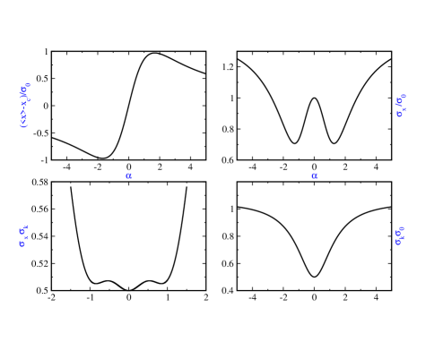
Figure 6: (Color online) $\langle x\rangle$, $\sigma_{x}$, $\sigma_{k}$ and $\sigma_{x}\sigma_{k}$ versus $\alpha$ for the initial non-Gaussian wave packet.

One clearly sees that $\sigma_{x}$, $|\phi(k)|^{2}$ and $\sigma_{k}$ are even functions of $\alpha$. The function $\rho(k)=|\phi(k)|^{2}$ is symmetric around central wave number $k_{0}$; and this point is a global maximum for $-\alpha_{0}<\alpha<\alpha_{0}$ while is a local minimum for $\alpha<-\alpha_{0}$ or $\alpha_{0}<\alpha$, where $\alpha_{0}=2\sqrt{2}\exp{[\pi^{2}/16]}/\pi=1.66836$. In Figure 6 the expectation value of position, uncertainty in position, uncertainty in momentum and the product of uncertainties versus $\alpha$ are plotted. Finally, the propagation of the above non-Gaussian packet in free space is given by

$$\psi(x,t) = \frac{1}{\left(2\pi\sigma_{0}^{2}\left[1+i\frac{\hbar t}{2m\sigma_{0}^{2}}\right]^{2}\right)^{1/4}}\frac{1}{\sqrt{1+\frac{\alpha^{2}}{2}(1-e^{-\pi^{2}/8})}}$$ (46)

$$\times \left[1+\alpha~{}e^{\frac{\pi^{2}}{16}\left(\frac{1}{1+i\frac{\hbar t}{2m\sigma_{0}^{2}}}-1\right)}\sin\left(\pi\frac{(x-x_{c})-ut}{4\sigma_{0}\left[1+i\frac{\hbar t}{2m\sigma_{0}^{2}}\right]}\right)\right]$$

$$\times \exp{\left\{ik_{0}\left[x-\frac{u}{2}t\right]\right\}}~{}\exp{\left\{-\frac{[(x-x_{c})-ut]^{2}}{4\sigma_{0}^{2}\left[1+i\frac{\hbar t}{2m\sigma_{0}^{2}}\right]}\right\}}~{}.$$

References

- (1) P. R. Holland 1993, The Quantum Theory of Motion (Cambridge: Cambridge University Press), chapter 6 and references therein
- (2) L. E. Ballentine 1998 Quantum Mechanics: A Modern Development (Singapore: World Scientific), chapter 14
-
(3)
D. Home 1997 Conceptual Foundations of Quantum Physics: An
Overview from Modern Perspectives (New York: Plenum), chapter 3 ;
D. Dürr, S. Goldstein and N. Zanghi 2013 Quantum Physics Without Quantum Philosophy (Berlin Heidelberg: Springer-Verlag) chapter 5 - (4) A. B. Nassar and S. Miret-Artés, Phys. Rev. Lett. 111, 150401 (2013)
- (5) R. P. Feynman, R. B. Leighton and M. Sands 1965 Lectures on Physics vol. III, Addison–Wesley, Reading, MA
- (6) F. Strocchi, Rev. Mod. Phys. 38 (1966) 36
- (7) A. Heslot, Phys. Rev. D 31 (1985) 1341
- (8) H-T. Elze Phys. Rev. A 85 (2012) 052109
- (9) L. Fratinoa, A. Lampob and H.-T. Elze (2014) arXiv:1408.1008
- (10) A. Lampo, L. Fratino and H.-T. Elze (2014) arXiv:1410.4472
- (11) D. Home, A. K. Pan and A. Banerjee J. Phys. A 42 (2009) 165302
- (12) N. Riahi J. Phys. A 46 (2013) 208001
- (13) D. Home, A. K. Pan and A. Banerjee J. Phys. A 46 (2013) 208002
- (14) N. Rosen, Am. J. Phys. 32 (1964) 377
- (15) N. Rosen, Am. J. Phys. 33 (1965) 146
-
(16)
C. Cohen-Tannoudji, B. Diu, F. Lalöe, 1977 Quantum
Mechanics (Paris: Wiley);
A.E. Bernardini, Ann. Phys. 324 (2009) 1303 - (17) H. G. Winful, Phys. Rep. 436 (2006) 1
- (18) P. R. Holland 1993, The Quantum Theory of Motion (Cambridge: Cambridge University Press) pp 55-61
- (19) J. G. Muga and C. R. Leavens Phys. Rep. 338 (2000) 353
- (20) P. R. Holland Phys. Rev. A 60 (1999) 4326
- (21) W. Struyve, W. De Baere, J. De Neve and S. De weird Phys. Lett. A 322 (2004) 24
- (22) P. Chowdhury, D. Home, A. S. Majumdar, S. V. Mousavi, M. R. Mozaffari and S. Sinha Class. Quantum Grav. 29 (2012) 025010
- (23) V. Zelevinsky 2011, Quantum Physics: From Time-Dependent Dynamics to Many-Body Physics and Quantum Chaos (Weinheim: Wiley-VCH), page 393