“Magic” Numbers in Smale’s 7th Problem

Abstract

This paper inquires into the concavity of the map $N\mapsto v_{s}(N)$ from the integers $N\geq 2$ into the minimal average standardized Riesz pair-energies $v_{s}(N)$ of $N$-point configurations on the sphere $\mathbb{S}^{2}$ for various $s\in\mathbb{R}$. The standardized Riesz pair-energy of a pair of points on $\mathbb{S}^{2}$ a chordal distance $r$ apart is $V_{s}(r)=s^{-1}\left(r^{-s}-1\right)$, $s\neq 0$, which becomes $V_{0}(r)=\ln\frac{1}{r}$ in the limit $s\to 0$. Averaging it over the $\left(\hskip-4.0pt\begin{array}[]{c}N\\ 2\end{array}\hskip-4.0pt\right)$ distinct pairs in a configuration and minimizing over all possible $N$-point configurations defines $v_{s}(N)$. It is known that $N\mapsto v_{s}(N)$ is strictly increasing for each $s\in\mathbb{R}$, and for $s<2$ also bounded above, thus “overall concave.” It is (easily) proved that $N\mapsto v_{-2}(N)$ is even locally strictly concave, and that so is the map $2n\mapsto v_{s}(2n)$ for $s<-2$. By analyzing computer-experimental data of putatively minimal average Riesz pair-energies $v_{s}^{x}(N)$ for $s\in\{-1,0,1,2,3\}$ and $N\in\{2,...,200\}$, it is found that the map $N\mapsto{v}_{-1}^{x}(N)$ is locally strictly concave, while $N\mapsto{v}_{s}^{x}(N)$ is not always locally strictly concave for $s\in\{0,1,2,3\}$: concavity defects occur whenever $N\in{\cal C}^{x}_{+}(s)$ (an $s$-specific empirical set of integers). It is found that the empirical map $s\mapsto{\cal C}^{x}_{+}(s),\ s\in\{-2,-1,0,1,2,3\}$, is set-theoretically increasing; moreover, the percentage of odd numbers in ${\cal C}^{x}_{+}(s),\ s\in\{0,1,2,3\}$ is found to increase with $s$. The integers in ${\cal C}^{x}_{+}(0)$ are few and far between, forming a curious sequence of numbers, reminiscent of the “magic numbers” in nuclear physics. It is conjectured that these new “magic numbers” are associated with optimally symmetric optimal-log-energy $N$-point configurations on $\mathbb{S}^{2}$. A list of interesting open problems is extracted from the empirical findings, and some rigorous first steps toward their solutions are presented. It is emphasized how concavity can assist in the solution to Smale’s $7$th Problem, which asks for an efficient algorithm to find near-optimal $N$-point configurations on $\mathbb{S}^{2}$ and higher-dimensional spheres.

 Typeset in LaTeX by the authors. To appear in Journal of Statistical Physics under the title: Optimal $N$-Point Configurations on the Sphere: “Magic” Numbers and Smale’s 7th Problem
In celebration of Doron Zeilberger’s $(1+\surd\epsilon)\cdot 60$-th birthday.

©2014 The authors. This preprint may be reproduced for noncommercial purposes.

1 Introduction

In various fields of science, ranging from biology over chemistry and physics to computer science, one encounters $N$-point optimization problems for which the following one is archetypical. Consider $N\geq 2$ distinct points on the two-sphere $\mathbb{S}^{2}$. Any such $N$-point configuration will be denoted by $\omega_{N}\subset\mathbb{S}^{2}$. The positions of the $N$ points are conveniently given by vectors ${\boldsymbol{{q}}}_{k}\in\mathbb{R}^{3}$ of Euclidean length $|{\boldsymbol{{q}}}_{k}|=1$, $k=1,\dots,N$, so that $\left|{\boldsymbol{{q}}}_{i}-{\boldsymbol{{q}}}_{j}\right|$ is the chordal distance between the two points in the pair $(i,j)$. Any pair $(i,j)$ is now assigned a standardized Riesz pair-energy $V_{s}(\left|{\boldsymbol{{q}}}_{i}-{\boldsymbol{{q}}}_{j}\right|)$, with

$$V_{s}(r) \equiv s^{-1}\left(r^{-s}-1\right),\qquad s\in\mathbb{R},\quad s\neq 0;$$ (1)

$$V_{0}(r) \equiv -\ln{r}\qquad\qquad\qquad\Big{(}\!\!=\lim_{s\rightarrow 0}V_{s}(r)\Big{)}.$$ (2)

The average standardized Riesz pair-energy of a configuration is given by

$$\langle V_{s}\rangle(\omega_{N})\equiv\frac{2}{N(N-1)}\;\sum\sum\limits_{\hskip-17.07182pt1\leq i<j\leq N}V_{s}(|{\boldsymbol{{q}}}_{i}-{\boldsymbol{{q}}}_{j}|),$$ (3)

and the minimal average standardized Riesz pair-energy by

$$v_{s}(N)\equiv\inf_{\omega_{N}\subset\mathbb{S}^{2}}\langle V_{s}\rangle(\omega_{N}).$$ (4)

The problem is to determine $v_{s}(N)$ together with the minimizing configuration(s) $\omega_{N}^{s}$ (also known as $N$-tuple of elliptic $s$-Fekete points) whenever such exist. For the convenience of the non-expert reader, in our Appendix A we present a brief survey of this intriguingly beautiful and rich, but also challengingly hard mathematical problem to which nobody knows the general solution. Only for one distinguished value of $s$ has this problem been solved for all $N$, and only for a few $N$-values has it been conquered for all $s$. Also computers are soon overwhelmed when $N$ becomes large.

Indeed, as apparently first noticed in [ErHo97], computer-assisted searches (see, e.g., [RSZ94], [RSZ95], [Aetal97], [Petal97], [ErHo97],  [BCNT02], [BCNT06], [Betal07],

[WaUl06], [WMA09]) for the minimizing configuration(s) suggest that the number of local minimum energy configurations (most of which are not globally minimizing) grows exponentially with $N$. An exponential proliferation of local minimizers, and by implication of critical points, eliminates the possibility of a polynomial-in-$N$ algorithm which first solves the algebraic problem of finding all critical points, then evaluates their energies, and finally picks the lowest energy configuration(s) amongst all critical points. Since it is so difficult to find the optimizing configurations, one may need to settle for less and employ computer-assisted (random) searches. Unfortunately, with increasing likelihood when $N$ becomes large a practically feasible random search will find only one of these exponentially many non-global minima without guarantee of its energy being close to the optimum. This is not good enough. What one wants is a controlled approximation. Smale’s 7th Problem [Sma98] is formulated in this spirit:

     

Find an algorithm which, upon input $N$, in polynomial time returns a configuration $\omega_{N}$ on $\mathbb{S}^{2}$ whose average standardized Riesz pair-energy does not deviate from the optimal value obtained with $\omega_{N}^{s}$ by more than a certain conjectured $s$-specific function of $N$.

     

Remark 1.

Smale’s problem was originally posed for $s=0$, viz. $V_{0}(r)=-\ln r$, and then not for the average logarithmic pair-energy but for the total logarithmic energy of the $N$-point configurations, i.e. for ${\mathcal{E}}_{0}(N)=$$\left(\hskip-4.0pt\begin{array}[]{c}N\\ 2\end{array}\hskip-4.0pt\right)$$v_{0}(N)$. The “$s$-specific function of $N$” in this original formulation is the fourth term of the partially proved, partially conjectured large-$N$ asymptotic expansion of the optimal logarithmic energy of $N$-point configurations on $\mathbb{S}^{2}$ [RSZ94, RSZ95],

$${\mathcal{E}}_{0}(N)=aN^{2}+bN\ln N+cN+d\ln N+\mathcal{O}(1),$$ (5)

with $a=\textstyle{\frac{1}{4}}\ln\textstyle{\frac{e}{4}}$ and $b=-\textstyle{\frac{1}{4}}$ rigorously known, and with rigorous upper and lower bounds on $c$, and numerical estimates for $d$, given in [RSZ94] (for an update, see [BHS12]). The coefficient “$d$” in Smale’s problem is unspecified and allowed to be bigger than any asymptotically determined “$d.\!$” 

Subsequently Smale extended his problem to $s\in[0,2)$; and he remarked that analogous problems can be formulated for higher-dimensional spheres $\mathbb{S}^{\mathrm{d}},{\mathrm{d}}=3,4,...$.

To the best of our knowledge, no algorithm has yet been found which delivers what Smale is asking for. Instead, as already mentioned, when $N$ gets (too) large, random searches and educated guesses (inevitably also of the type “trial and error”) are employed which produce many different local energy minimizers for the same $N$, amongst which the one with the lowest energy is a putatively energy-optimizing configuration — until a better one is found eventually, perhaps. In this situation it becomes important to search for necessary criteria that can test those configurations, which have produced the lowest energy amongst all empirically found configurations with a given $N$, for their potential optimality. We emphasize that such types of tests can only identify non-optimal data, but not confirm optimal ones.

One such test, based on the strict monotonic increase of $N\mapsto{v}_{s}(N)$ (see [Lan72] for a proof), was proposed and carried out successfully in [Kie09b]. There, about two dozen experimentally found putatively minimal energies ${v}_{s}^{x}(N)$ were identified, in publically available lists of empirical data, at which the empirical map $N\mapsto{v}_{s}^{x}(N)$ failed to be monotonically increasing — hence, these data could not possibly be true minimal energies $v_{s}(N)$, making it plain that it was / is worth an effort to do better.

Of course, all empirical maps $N\mapsto v_{s}^{x}(N)$ which we analyzed in this paper we also tested for whether they strictly increase — all data passed this first derivative test.

Remark 2.

Incidentally, also the map $s\mapsto v_{s}(N)$ is strictly monotonically increasing (see Appendix C for a proof), supplying another necessary criterion for optimality of putative standardized Riesz pair-energy minimizers. All empirical maps $s\mapsto v_{s}^{x}(N)$ which we analyzed in this paper we also tested for whether they strictly increase — all data passed this first derivative test, too.

The main purpose of the present paper is to report the results of our quest for additional tests in form of necessary criteria for minimality, based not on the first, but on the second discrete derivative of $N\mapsto{v}_{s}(N)$. Our point of departure was the observation that strict monotonic increase of $N\mapsto v_{s}(N)$ in concert with its boundedness above for $s<2$ (a simple variational estimate) implies that the overall shape of the graph $\{(N,v_{s}(N)):N=2,3,....\}$ must be “concave in the large” for each $s<2$. This raised the question whether this graph is perhaps even locally, at each $N>2$, strictly concave when $s<2$. Moreover, although $v_{s}(N)$ is not bounded above for $s\geq 2$, the leading-order terms of the asymptotic large-$N$ expansion of $v_{s}(N)$, namely $v_{2}(N)\propto\ln N$ [KuSa98] and $v_{s}(N)\propto N^{(s-2)/2}$ for $s>2$ [HaSa05], are strictly locally concave for $2\leq s<4$, so that it was even conceivable that so was $N\mapsto v_{s}(N)$. So the question we asked ourselves was whether the discrete second derivative of $v_{s}(N)$, given by

$$\ddot{v}_{s}(N)=v_{s}(N-1)-2v_{s}(N)+v_{s}(N+1),\qquad N>2,$$ (6)

is perhaps strictly negative for all $N>2$ when $s<2$ (or possibly even when $s\leq 4$). Clearly, knowledge of any $s$-values for which the map $N\mapsto{v}_{s}(N)$ is everywhere strictly concave will yield a necessary criterion for minimality that can be fielded as a test for lists of empirical data of those putatively minimal Riesz $s$-energies.

Remark 3.

As with Smale’s 7th problem, analogous concavity questions can be raised about the minimal average Riesz $s$-energy $v_{s}(N)$ for the higher-dimensional spheres $\mathbb{S}^{\rm d}$, $\rm d=3,4,...$, and also for the circle $\mathbb{S}^{1}$ (although no optimality test for putative minimizers on $\mathbb{S}^{1}$ is needed — all optimizers with $N\geq 2$ and $s\geq-2$ are explicitly known, see [BHS09]). Interestingly enough, for the problem on $\mathbb{S}^{1}$ the $N$-dependence of $N\mapsto v_{s}(N)$ is polynomial for special $s$-values [Bra11] — in particular, the map $N\mapsto v_{2}(N)$ is affine linear; furthermore, our own partly analytical / partly numerical studies of the explicit finite sum formulas for ${v}_{s}(N)$ strongly support the conjecture that $N\mapsto v_{s}(N)$ is locally strictly concave for $s\in(-2,2)$ and locally strictly convex for $s>2$, indeed!

What we found out about the minimal average Riesz $s$-energy ${v}_{s}(N)$ for $\mathbb{S}^{2}$ — mostly empirically yet partly rigorously — went beyond our expectations, including not only strict concavity of the theoretical map $N\mapsto{v}_{s}(N)$, respectively the empirical map $N\mapsto{v}_{s}^{x}(N)$, for some $s$-values, but also hints at a monotonic increase with $s$ of the set of convexity points whenever concavity of ${v}_{s}^{x}(N)$ failed, suggesting novel and unexpected test criteria for optimality! In particular, the hypothesis that the empirically suggested monotonicities are factual has led us to discover in a published data list three non-optimal data points which had not previously been detected.

More precisely, we readily affirmed the strict concavity of $N\mapsto{v}_{s}(N)$ for the special value $s=-2$, for which the problem of the elliptic $s$-Fekete points is exactly solvable for all $N$; cf. Appendix A. Thus, simply by differentiating the expression (109) for $v_{-2}(N)$ twice one gets a strictly negative expression for the second discrete derivative. Furthermore, twofold discrete differentiation of $v_{s}(2n)$ when $s<-2$ (see (110)) showed that also $2n\mapsto v_{s}(2n)$ is strictly locally concave for $s<-2$; of course, this does not prove that $N\mapsto v_{s}(N)$ is strictly concave for all $N>2$ when $s<-2$, but it suggests that one may be able to prove it rigorously. This already exhausts the $s$-values for which we were able to rigorously prove some strict local concavity result. Unfortunately, the regime $s\leq-2$ is of rather academic interest — in particular, for the exactly solvable case $s=-2$ one does not need any necessary criteria for minimality to test putative optimizers! The practically interesting regime is $s>-2$.

In the absence of any closed form expressions of $v_{s}(N)$ for $s>-2$ we decided to gather some experimental input and turned to the empirical data published in [ErHo97, HSS94, RSZ95, Cal09], and [WaUl], and to those publicly available at the website [BCGMZ] (some of which we generated ourselves). By carefully scrutinizing these data lists we discovered that strict local concavity of $N\mapsto v_{s}(N)$ may in fact hold for $s=-1$, but not for $s\in\{0,1,2,3\}$ — we then proved, quasi-rigorously for $s\in\{0,1,2,3\}$, rigorously for $s\geq 10$, that local concavity of $N\mapsto v_{s}(N)$ fails.

We then inspected the sets of the $N$-values at which $\ddot{v}_{s}^{x}(N)\geq 0$ more closely. Empirically we found that these sets were set-theoretically increasing with $s$ — except for two relatively large $N$-values, namely $N=177$ and $N=197$, when $s$ was 2 or 3. Since the empirical data become less trustworthy the larger $N$ becomes, and also the larger $s$ becomes, we used the “Thomson applet” at [BCGMZ] to see whether we could find configurations with lower energy using an “educated guess” as input configuration for $N=177$ and $N=197$. Happily we succeeded, and when we used these better energy data points for $N=177$ and $N=197$ at $s=2$, respectively 3, those $N$-values were no longer exceptions to the empirical overall monotonic increase of the sets of the $N$-values at which $\ddot{v}_{s}^{x}(N)\geq 0$.

To summarize, we have collected empirical evidence for the following conjectures:

Conjecture 1.

The map $N\mapsto v_{-1}(N)$ is locally strictly concave for all $N>2$.

Conjecture 2.

When $s\in\{0,1,2,3\}$ the map $N\mapsto v_{s}(N)$ is not locally strictly concave, and the set of $N$-values at which strict concavity fails is expanding with $s$.

Clearly, if proven true, these regularities will serve as useful test criteria for optimality of empirical large $N$-configurations at the above $s$-values. Yet our empirical findings also suggest a catalog of interesting new questions for general $s$-values.

A Catalog of Interesting Questions (and some Partial Answers)

To pose our questions sharply, we define several new quantities. First of all, for each $s$ we partition the integer subset $\{N>2\}$ into three mutually disjoint subsets: the set of strict local concavity ${\cal C}_{-}(s)$, the set of strict local convexity ${\cal C}_{+}(s)$, and the set of local linearity ${\cal C}_{0}(s)$, defined as

$${\cal C}_{-}(s) \equiv\{N>2|\ddot{v}_{s}(N)<0\},$$ (7)

$${\cal C}_{+}(s) \equiv\{N>2|\ddot{v}_{s}(N)>0\},$$ (8)

$${\cal C}_{0\,}(s) \equiv\{N>2|\ddot{v}_{s}(N)=0\},$$ (9)

respectively. We note that ${\cal C}_{-}(s)\cup{\cal C}_{0}(s)\cup{\cal C}_{+}(s)=\{N>2\}$. We are now ready to raise our first mathematical question.

Empirically we found that ${\cal C}_{+}^{x}(0)\subset{\cal C}_{+}^{x}(1)\subset{\cal C}_{+}^{x}(2)\subset{\cal C}_{+}^{x}(3)$. Thus we ask:

1. Is $s\mapsto{\cal C}_{+}(s),s\!\in\!\mathbb{R}$, monotonic increasing in the sense of set-theoretic inclusion?

If the answer to Q 1 is affirmative, then this set-theoretical monotonicity supplies a potentially useful test for optimality of putative energy minimizers for any real $s$, not just for the handful of integer $s$-values which we have studied empirically. In particular, it would imply that ${\cal C}_{+}(s)=\emptyset$ for all $s\leq-2$ (for ${\cal C}_{+}(-2)=\emptyset$), and even for all $s\leq-1$ if Conjecture 1 is true. More precisely, an affirmative answer to Q 1 would imply that for some $s_{*}\geq-2$ one has ${\cal C}_{+}(s)=\emptyset$ whenever $s\leq s_{*}$.

Incidentally, by itself this would not yet imply strict local concavity of the map $N\mapsto v_{s}(N)$ for $s<s_{*}$, only local concavity, because we cannot conclude that ${\cal C}_{0}(s)$ would be empty for all $s<s_{*}$; yet we suspect that in fact ${\cal C}_{0}(s)=\emptyset$ for all $s<s_{*}$.

To address the question of strict local concavity of $N\mapsto v_{s}(N)$ independently of whether or not the answer to Q 1 is affirmative, we define $s_{*}$ as follows,

$$s_{*}\equiv\sup\{s^{\prime}|{\cal C}_{0}(s)\cup{\cal C}_{+}(s)=\emptyset\ \forall\ s\leq s^{\prime}\}.$$ (10)

Note that the “sup” cannot be a “max” because for any fixed configuration $\omega_{N}$ the map $s\mapsto\langle V_{s}\rangle(\omega_{N})$ is a $C^{\infty}$ function, which implies that the map $s\mapsto v_{s}(N)$ is a $C^{0}$ function. ($C^{\infty}$ regularity of $s\mapsto v_{s}(N)$ should hold almost everywhere, but for each $N>2$ the minimizing configuration may change discontinuously at some $s$-value(s), at which only $C^{0}$ regularity can be guaranteed.) Alternatively, $s_{*}$ is defined as

$$s_{*}\equiv\inf\{s|\text{ $\ddot{v}_{s}(N)\geq 0$ for at least one $N>2$}\},$$ (11)

and “$\inf{}=\min{}$” if and only if $s_{*}>-\infty$. Thus we ask:

1. Is $s_{*}>-\infty$?

2. If $s_{*}>-\infty$, then what is the value of $s_{*}$?

Because of the strict local concavity of the maps $N\mapsto v_{-2}(N)$ and $2n\mapsto v_{s}(2n)$ for $s<-2$, we not only suspect that $s_{*}>-\infty$, but that $s_{*}\geq-2$. In fact, the strict local concavity of the empirical map $N\mapsto v_{-1}^{x}(N)$ even suggests that $s_{*}\geq-1$, while the violations of strict local concavity by the empirical map $N\mapsto v_{0}^{x}(N)$ suggest that $s_{*}<0$. If confirmed that $s_{*}\in(-2,0)$, strict local concavity of $N\mapsto v_{s}(N)$ can be fielded as rigorous test criterion for optimality of putative optimizers for $s\in(-\infty,s_{*})$, even though only $s\in(-2,s_{*})$ would seem to be of practical interest.

If $s_{*}>-\infty$, then ${\cal C}_{+}(s)=\emptyset$ for $s\leq s_{*}$, and ${\cal C}_{0}(s)=\emptyset$ for $s<s_{*}$ but not for $s=s_{*}$. This leads us to now define the critical set of local linearity,

$${\cal L}_{*}\equiv{\cal C}_{0}(s_{*})\ (\mbox{if}\ s_{*}>-\infty).$$ (12)

Assuming that $s_{*}>-\infty$, we now expand our list of mathematical questions:

1. Is the set ${\cal L}_{*}$ finite or infinite?

2. Can one explicitly compute the set ${\cal L}_{*}$?

3. Which optimal configurations correspond to the set ${\cal L}_{*}$?

Again supposing that $s_{*}>-\infty$, there are then also interesting questions to ask about the regime $s>s_{*}$. In particular, since $\mathbb{N}$ is countable while $\mathbb{R}$ is not, the continuity of $s\mapsto\ddot{v}_{s}(N)$ suggests that ${\cal C}_{0}(s)$ is empty almost everywhere (w.r.t. Lebesgue measure). Thus it is natural to ask:

1. Is the set of $s$-values for which ${\cal C}_{0}(s)\neq\emptyset$ finite or infinite?

2. Can one compute the set of $s$-values at which ${\cal C}_{0}(s)\neq\emptyset$?

As with ${\cal L}_{*}$, one can raise similar questions for all non-empty ${\cal C}_{0}(s)$, thus

1. For each non-empty ${\cal C}_{0}(s)$: is it finite or infinite?

2. For each non-empty ${\cal C}_{0}(s)$: can one compute it?

3. For each non-empty ${\cal C}_{0}(s)$: which configurations does it represent?

Questions Q 2 – Q11 do not presuppose that Q 1 is answered affirmatively. Yet if the answer to Q 1 is affirmative, then both $\lim_{s\to-\infty}{\cal C}_{+}(s)\equiv{\cal C}_{+}(-\infty)$ and $\lim_{s\to\infty}{\cal C}_{+}(s)\equiv{\cal C}_{+}(\infty)$ exist. In particular, then ${\cal C}_{+}(-\infty)=\emptyset={\cal C}_{+}(s)\;\forall s\leq s_{*}$, with $s_{*}\geq-2$, as we already know. As for the opposite limit, since the large-$N$ asymptotics of ${v}_{s}(N)$ is locally strictly convex for $s>4$ [HaSa05], it is tempting to speculate whether there exists $s^{*}<\infty$ such that the map $N\mapsto{v}_{s}(N)$ itself is locally strictly convex for all $s>s^{*}$, which would mean that ${\cal C}_{+}(\infty)=\mathbb{N}\setminus\{1,2\}={\cal C}_{+}(s)\;\forall\;s>s^{*}$; equivalently, ${\cal C}_{-}(s)=\emptyset$ for all $s\geq s^{*}$. However, we shall provide partly rigorous, partly numerical evidence for ${\cal C}_{+}(\infty)\neq\mathbb{N}\setminus\{1,2\}$. So ${\cal C}_{+}(\infty)$, if it exists, is likely more complicated, and more interesting than the full set of admissible integers $\mathbb{N}\setminus\{1,2\}$. Thus, under the hypothesis that Q 1 is answered affirmatively, we also ask:

1. Can one explicitly characterize ${\cal C}_{+}(\infty)$?

Finally, the question of $s^{*}$ persists:

1. Does there exist an $s^{*}<\infty$ such that ${\cal C}_{+}(s)={\cal C}_{+}(\infty)$ for all $s>s^{*}$?

2. If yes, can one compute $s^{*}<\infty$?

All these questions are presumably quite difficult to answer. In any event, it is reasonable to expect valuable insights even from partial answers. For example, to answer Q 2, and also Q 3 conditional on an affirmative answer for Q 2, one may want to try proving a negative upper bound on $\ddot{v}_{s}(N)$ for all $s$ below some critical value. Any upper bound on $\ddot{v}_{s}(N)$ obtained in the process, even if not negative, would offer a test criterion for optimality. In this vein, in subsection 4.2 of this paper we prove the following bounds:

Proposition 1.

For $s<0$ the second discrete derivative of $v_{s}(N)$ is bounded above and below as follows,

$$\frac{2}{(N+1)(N-2)}\left(v_{s}(N)+\frac{1}{s}\right)\leq\ddot{v}_{s}(N)\leq-\frac{2}{(N+1)N}\left(v_{s}(N)+\frac{1}{s}\right).$$

Of course, our Proposition 1 is not strong enough to offer an answer even to Q 2.

Coming to Q 3, we will provide some (quasi-)rigorous upper bounds on $s_{*}$. We already mentioned that the large-$N$ asymptotics of the map $N\mapsto{v}_{s}(N)$ is strictly convex for $s>4$ [HaSa05], which implies that $s_{*}\leq 4$; yet, empirically from the analysis of putative minimizers we expect that $s_{*}<0$. Indeed, with the help of the partly empirically / partly rigorously known optimizers for $N\in\{5,7\}$ in the range $s\in[0,2)$ and the rigorously known optimizer for $N=6$, in subsection 3.5 we will prove the following:

Proposition 2.

Under the assumption that for $N\in\{5,7\}$ the optimizing configurations in the range $s\in[0,2)$ are given by the regular triangular and pentagonal bi-pyramids, respectively, one has $s_{*}<0.$

We will rigorously prove Proposition 2; yet the bound on $s_{*}$ in Proposition 2 is called quasi-rigorous, for the named configurations are not rigorously known to be optimizers for all $s\in[0,2)$, although there can be hardly any doubt that they are.

With the help of the rigorously known optimizing configurations for $N\in\{4,6\}$ and the only partly rigorously known, hence putatively optimizing configurations for $N=5$ in the respective ranges $s\in(-2,s^{\dagger}]$ and $s\in[s^{\dagger},\infty)$, with $s^{\dagger}=15.04807...$, in subsection 4.4 we will also supply partly rigorous and partly numerical evidence for

Conjecture 3.

Under the assumption that the optimizing configurations for $N=5$ in the range $s\in(-2,\infty)$ are given by the regular triangular bi-pyramid (when $s\leq s^{\dagger}$) and the square pyramid with adjusted height (when $s\geq s^{\dagger}$), we have that

$$\forall\;s\in(-2,\infty):\quad\ddot{v}_{s}(5)<0.$$

Thus, while it is locally strictly concave for $s=-2$ and presumably for all $s\leq-2$, and possibly for all $s\leq-1$, the map $N\mapsto{v}_{s}(N)$ is very likely not locally strictly convex for any $s$ — even though its large-$N$ asymptotics is, when $s>4$. So as for Q12, very likely ${\cal C}_{+}(\infty)$ (if it exists) is not $\mathbb{N}\setminus\{1,2\}$.

We have mentioned large-$N$ asymptotics several times already. We ourselves shall produce several well-motivated conjectures that relate the concavity of $N\mapsto{v}_{s}(N)$ to its asymptotics at large $N$ for which even computer-assisted searches of the optimal $N$-point configurations are hopeless. We defer stating our conjectures to Section 5, for we need technical preparations beyond the scope of this introduction.

Our last remark makes it plain that we consider our mathematical questions to be of theoretical interest in their own right, too, irrespective of whether some test for empirical data will ensue from their answers or not. In this spirit we also raise an intriguing question which cannot be so sharply formulated:

“Magic” numbers: “Optimally optimal” configurations?

For $s=0$, the smallest $s$-value for which we found empirical violations of strict local $N$-concavity, i.e. for the logarithmic pair interaction invoked in the original formulation of Smale’s $7$th Problem, the violations of strict local concavity were few and far between. They occurred at the following experimental sequence of integers:

$${\cal C}_{+}^{x}(0)=\big{\{}\underline{6},\underline{12},\underline{24},32,\underline{48},\underline{60},67,\underline{72},80,104,\underline{108},122,\underline{132},137,...\big{\}}.$$ (13)

Curiously, the majority of the numbers in the sequence (13) are multiples of $6$ (underlined), or almost multiples (like $67$ and $137$) — coincidence?

We note that the logarithmic-energy minimizers for the first two “integers of convexity,” i.e. $N=6$ and $N=12$, are two “optimally symmetric” configurations, namely Platonic polyhedra: the octahedron ($N=6$) and icosahedron ($N=12$); also the (putative) minimizers for $N\in\{24,48,60\}$ are highly symmetric configurations; in particular, the one for $N=24$ is an Archimedean polyhedron (also for $N\in\{48,60\}$ there are Archimedean polyhedra, but these are NOT log-energy optimizers). To be sure, there is an integer inbetween which is not divisible by $6$, namely $N=32$ (the highly symmetric optimizer is a Catalan polyhedron), and also the “odd-balls” $N=67$ and (of all integers!) $N=137$ show up.

Yet, assuming that ${\cal C}_{+}^{x}(0)={\cal C}_{+}(0)$, it is an intriguing thought that the $N$-values in ${\cal C}_{+}(0)$ may correspond to $\log$-energy-optimizing configurations which are “optimally symmetric” in the following sense. Most of the $\log$-energy-optimizing configurations associated with ${\cal C}_{+}^{x}(0)$ are separated by longer $N$-intervals in which $N\mapsto v_{0}^{x}(N)$ is strictly concave. This suggests that, perhaps, the configurations in an interval of concavity form a family of more-and-more symmetric optimizers which better-and-better approximate a highly symmetric endpoint configuration. Once an endpoint configuration is reached, the addition of the next point inevitably will destroy a high amount of symmetry, for which an extra large amount of energy may be required.

These “concave families” would thus be vaguely analogous to the “periods” in the so-called periodic table of the chemical atoms. The endpoints of the periods are the chemically very inert noble gases which are associated with highly symmetric “electronic configurations” about the nuclei with charge number $Z\in\{2,10,18,...\}$. Incidentally, also the atomic nuclei seem to form something akin to “periods,” in the sense that the set of nucleon numbers $\{2,8,20,28,50,82,126,...?...\}$ is associated with nuclei that have a particular high binding energy per nucleon. This set of nucleon numbers is known as the Magic Numbers of nuclear physics. By analogy, we call the set ${\cal C}_{+}(0)$ (for now: ${\cal C}^{x}_{+}(0)$) the “Magic Numbers of Smale’s 7th Problem.”

The structure of the remaining sections

     

• In Section 2 we present the details of our analysis of the data of [HSS94, RSZ95, Cal09, BCGMZ, WaUl], which induced us to formulate questions Q 1 – Q14.

• In Section 3 we address Q 3, obtaining (quasi-)rigorous upper bounds on $s_{*}$. More to the point, we give a computer-assisted proof of Proposition 2. For this we explicitly compute the (putative) expressions for $s\mapsto\ddot{v}_{s}(N)$ for $N\in\{3,4,5,6\}$ when $s$ runs through certain intervals in which these functions are elementary, easily discussed, and readily evaluated with maple, mathematica, or matlab. With the help of the exactly computable $s\mapsto\ddot{v}_{s}(3)$ we also show rigorously that ${\cal C}_{+}(s)$ is nonempty whenever $s\geq 10>s_{*}$.

• In Section 4 we prove various rigorous upper and lower bounds on $\ddot{v}_{s}(N)$ which go to zero like a power of $N$ when $N\to\infty$ and $s<0$. In particular, we prove Proposition 1. We re-emphasize that our upper and lower bounds can serve for testing optimality of putative energy minimizers. While our rigorous bounds are not strong enough to prove negativity of $\ddot{v}_{s}(N)$ uniformly in $N>2$ for any $s>-2$, we do rigorously prove negativity of $\ddot{v}_{s}(N)$ for $N\in\{4,6\}$ in some regime of negative $s$-values $>-2$ by taking advantage of the explicitly known optimizers for these $N$-values (and for $N=2$). We also obtain a rigorous upper bound for $s\mapsto\ddot{v}_{s}(12)$, but this bound is positive because the control of the opitimizers for $N\in\{11,13\}$ is too weak. We also vindicate Conjecture 3.

• In Section 5 we present an asymptotic analysis of $N\mapsto\ddot{v}_{s}(N)$ for the large-$N$ regime and produce several well-motivated conjectures that relate the concavity of $N\mapsto{v}_{s}(N)$ to the large-$N$ asymptotics. The character of the asymptotics depends on whether $s$ is in the potential regime $s\in(-2,2)$, in the hypersingular regime $s>2$, or exactly inbetween — at the singular $s=2$. A discussion of the “degeneracy regime” $s\leq-2$ will be left for some future work.

• In Section 6 we summarize our findings and suggest future inquiries.

• In Appendix A we briefly survey some distinguished minimal Riesz $s$-energy problems for $N$-point configurations on $\mathbb{S}^{2}$ and the pertinent literature.

• In Appendix B we prove relations (111) and (112) needed in Appendix A.

• In Appendix C we prove the strict monotonic increase of $s\mapsto{v}_{s}(N)$.

• In Appendix D we include a brief study of data of spherical digital nets.

2 Data analysis for $s\in\{-1,0,1,2,3\}$ and $N\leq 200$

There are many studies of putatively minimal standardized Riesz $s$-energies, but only a few feature data lists for consecutive $N$-values which are sufficiently long for our purposes. In [ErHo97] the first 110 consecutive data for the Thomson problem ($s=1$) are reported; similarly, on the website [HSS94] the first 130 consecutive data for $s=1$ are listed, and on the website [WaUl06], 391 consecutive data for $s=1$, starting with $N=10$, are reported — all these are never worse than those of [ErHo97]. In [RSZ95] one finds the first 200 consecutive data for $s\in\{-1,0,1\}$, and these authors remark that their data for $s=1$ agree with those of [HSS94] for the same $N$-values. M. Calef in his thesis [Cal09] lists 180 consecutive data for minimizing configurations, starting at $N=20$, covering the cases $s\in\{0,1,2,3\}$; he also identified the number of “stable” configurations observed during many trials. In $16$ cases the obtained results for $s=0$ and $1$ differed by more than $10^{-6}$ compared to results in [RSZ95] ($s=0$ and $1$) and [MDH96] ($s=1$), some lower and some higher than those of these other two works. On the interactive website [BCGMZ] putatively minimal Riesz energies are reported for $s\in\{0,1,\dots,12\}$, yet for variously many consecutive $N$-values. Although there one finds consecutive data for $s=0$ and $s=1$ up to $N$ in the thousands, data become less trustworthy with increasing $N$; yet whenever a user finds a lower-energy than previously observed, this new record holder is substituted for the old one.

We chose to work with about 200 numerical data each for $s\in\{-1,0,1,2,3\}$. In each case, we selected the lowest-energy data available from any of the mentioned lists. Thus, for $s\in\{-1,0,1\}$ we worked with the data from [RSZ95], except that for $s=0$ and $1$ we replaced a few data points by lower-energy data from [Cal09]; for $s=1$ they agree with those at [WaUl06]. For $s\in\{2,3\}$ and $N\in\{20,...,200\}$, we used the data from [Cal09], supplemented by data from [BCGMZ] for $s\in\{2,3\}$ and $N\in\{3,...,19\}$; however, for $s=3$ consecutive data were available at [BCGMZ] only for $N\in\{3,..,12\}$, together with data for $N\in\{16,18,19\}$. So we used the applet [BCGMZ] to create our own experimental $s=3$ data for $N\in\{13,14,15,17\}$. Moreover, we also used the applet [BCGMZ] to create our own experimental $s=2$ and $3$ data for $N=177$ and $197$, improving over those reported in [Cal09]; see below.

The experimental data ${\cal E}^{x}_{s}(N)$ reported in [RSZ95, Cal09, BCGMZ] (and in the other above-cited publications) have been computed with the conventional Riesz $s$-energy. We converted the data into putatively minimal average standardized Riesz pair-energies, using the formula $v^{x}_{s}(N)=\frac{1}{s}\big{(}\frac{2}{N(N-1)}{\cal E}^{x}_{s}(N)-1\big{)}$ for $s\in\{-1,1,2,3\}$; when $s=0$ only multiplication by $2/N(N-1)$ was required to obtain $v^{x}_{0}(N)$.

Since the forward derivative $N\mapsto\dot{v}_{s}^{+}(N)\equiv{v}_{s}(N+1)-{v}_{s}(N)$ is strictly increasing, for each $s\in\{-1,0,1,2,3\}$ we first checked whether $v^{x}_{s}(N+1)>v^{x}_{s}(N-n)$ for all $0\leq n\leq N-2$. All data that we pooled together for each $s$-value passed this test.

2.1 Plots of ${v}_{s}^{x}(N)$ and $\ddot{v}_{s}^{x}(N)$ vs. $N$

A first impression was gained by plotting $v_{s}^{x}(N)$ versus $N$ for $N\in\{2,\dots,200\}$ and $s\in\{-1,0,1,2,3\}$. The easy-to-prove ordering (see Appendix C)

$$v_{s}(N)>v_{t}(N)\quad\mbox{for}\quad s>t$$ (14)

suggested to us to plot all five graphs $(N,v_{s}^{x}(N))$, $s\in\{-1,0,1,2,3\}$, of the empirical data jointly into a single figure; see Fig. 1, which shows (a) the graph $(N,v_{-1}^{x}(N))$ computed with consecutive data for ${\cal E}^{x}_{-1}(N)$ from [RSZ95], (b) the graphs $(N,v_{0}^{x}(N))$ and $(N,v_{1}^{x}(N))$, both computed with consecutive data for ${\cal E}^{x}_{0}(N)$, respectively ${\cal E}^{x}_{1}(N)$, pooled from [RSZ95, Cal09], and (c) the graphs $(N,v_{2}^{x}(N))$ and $(N,v_{3}^{x}(N))$, both computed with consecutive data for ${\cal E}^{x}_{s}(N)$, $s\in\{2,3\}$, pooled from [Cal09] and [BCGMZ] (all data points with the same $s$-value are joined by thin solid lines to guide the eye). Fig. 1 reveals that $v^{x}_{-1}(N)<v^{x}_{0}(N)<v^{x}_{1}(N)<v^{x}_{2}(N)<v^{x}_{3}(N)$; thus, all empirical data that entered Fig. 1 pass the test implied by (14) (cf. Remark 2).

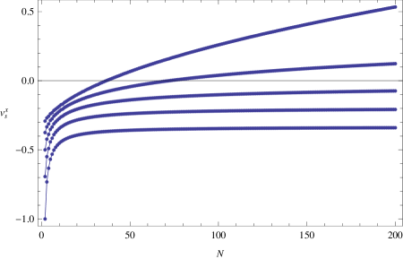
Figure 1: The empirical functions $v^{x}_{s}(N)$ vs. $N$ for $s\in\{-1,0,1,2,3\}$.

Fig. 1 reveals also that the five empirical graphs $N\mapsto v_{s}^{x}(N)$, $s\in\{-1,0,1,2,3\}$, are strictly increasing (as already mentioned above) and overall concave (as they should). Furthermore, to the human eye the empirical map $N\mapsto v_{s}^{x}(N)$ appears to be strictly locally concave for $s\in\{-1,0\}$, while convexity defects seem to occur for $s\in\{1,2,3\}$; interestingly, the online version of Fig. 1 allows one to zoom in, re-enforcing the impression about strict concavity vs. convexity defects. Of course, the human eye can only distinguish so much, so we next plotted the second discrete derivative $\ddot{v}_{s}^{x}(N)$ for $s\in\{-1,0,1,2,3\}$, and $N\in\{3,...,199\}$.

Shown in Fig. 2 is the graph $(N,\ddot{v}^{x}_{-1}(N))$ for $2<N<200$, together with a zoom-in of the domain $100\leq N<200$. (Since the amplitude of $\ddot{v}_{-1}^{x}(N)$ decays from about $10^{-1}$ to less than $10^{-6}$ when $N$ ranges from 3 to 199, no single plot can show the global structure of the graph as well as its fine structure.) The data $\ddot{v}^{x}_{-1}(N)$ in Fig. 2 remain below the $N$ axis, confirming the impression that $N\mapsto{v}^{x}_{-1}(N)$ is strictly locally concave.

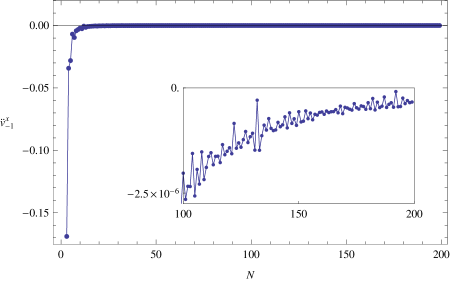
Figure 2: $\ddot{v}^{x}_{-1}(N)$ as a function of $N$. The solid line is drawn to guide the eye.

While Fig.s 1 and 2 do show strict local concavity of $N\mapsto v_{-1}^{x}(N)$, we also confirmed the optical impression of the strict local concavity of the empirical function $N\mapsto v^{x}_{-1}(N)$ with a refined data analysis; see below. The strict local concavity of $N\mapsto v_{-1}^{x}(N)$ for $2\leq N\leq 200$ can be taken as mild empirical support for our Conjecture 1 that $N\mapsto v_{-1}(N)$ is strictly locally concave.

Also the plot of $N\mapsto v_{0}^{x}(N)$ in Fig. 1 does look pretty much strictly concave everywhere; however, the graph of $N\mapsto\ddot{v}_{0}^{x}(N)$, shown in Fig. 3 for $N\in\{3,...,199\}$, reveals that the graph of $N\mapsto v_{0}^{x}(N)$ is not locally strictly concave! Despite the strictly concave optical appearance of $N\mapsto v_{0}^{x}(N)$, tiny violations of concavity occur every now and then, in fact already when $N$ is less than a dozen. The positivity of some small-$N$ data in the graph of $N\mapsto v_{0}^{x}(N)$ is clearly visible, but not for $N$ larger than a dozen (say), because the amplitude of $\ddot{v}_{s}^{x}(N)$ now decays from a value of order $10^{-1}$ to less than $10^{-5}$ when $N$ ranges from 3 to 199. To aid the visualization in the global graph, we plotted positive data points with black filled diamonds, negative ones with blue filled circles (colors online); again, we also inserted a zoom-in for the domain $100\leq N<200$ — note the different vertical scale.

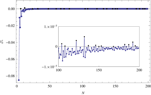
Figure 3: $\ddot{v}^{x}_{0}(N)$ as a function of $N$. The solid line is drawn to guide the eye.

We already mentioned that zooming into Fig. 1 reveals that neither of the graphs $N\mapsto v_{s}^{x}(N)$, $s\in\{1,2,3\}$, appears locally strictly concave, not even to the human eye. Indeed, the graphs $(N,\ddot{v}^{x}_{s}(N))$ for $N\in\{3,...,199\}$ and $s\in\{1,2,3\}$ clearly cross the $\ddot{v}^{x}_{s}(N)=0$ axis many times; see Fig.s 4, 5, and 6, which are designed like Fig. 3.

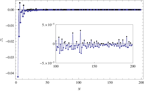
Figure 4: $\ddot{v}^{x}_{1}(N)$ as a function of $N$. The solid line is drawn to guide the eye.

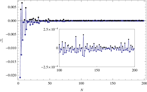
Figure 5: $\ddot{v}^{x}_{2}(N)$ as a function of $N$. The solid line is drawn to guide the eye.

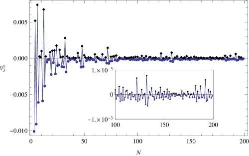
Figure 6: $\ddot{v}^{x}_{3}(N)$ as a function of $N$. The solid line is drawn to guide the eye.

Since the minimizing configurations for $N$ less than a dozen or so have been determined numerically with a high degree of confidence, the empirical violations of strict local concavity for $s\in\{0,1,2,3\}$ at the smaller $N$ values do not seem to be due to incorrect computations of the minimal average pair-energies.

2.2 The sets ${\cal C}_{+}^{x}(s)$

We next inspected the numerical data of the second discrete derivative $\ddot{v}_{s}^{x}(N)\equiv\dot{v}_{s}^{+}(N)-\dot{v}_{s}^{-}(N)$ (where $\dot{v}_{s}^{-}(N)\equiv{v}_{s}(N)-{v}_{s}(N-1)$ is the first backward derivative) for $N\in\{3,...,199\}$ and $s\in\{-1,0,1,2,3\}$. For each of these $s$-values we have collected the $N$-values at which $\ddot{v}_{s}^{x}(N)>0$ into the empirical set ${\cal C}_{+}^{x}(s)$.

Empirically, we thereby found the following experimental sets of convexity:

$${\cal C}_{+}^{x}(-1)=\emptyset,\phantom{nixxxxxxxxxxxxxxxxxxxxxxxxxxxxxxxxxxxxxxxxxx}$$ (15)

$${\cal C}_{+}^{x}(\;0\;)=\big{\{}6,12,24,32,48,60,67,72,80,104,108,122,132,\phantom{nixxxxxxx}\hfill$$ (16)

$$\phantom{6}137,146,150,153,168,182,187,192,195,...?...\big{\}},$$

$${\cal C}_{+}^{x}(\;1\;)=\big{\{}4,6,12,18,20,22,24,27,32,44,48,50,60,62,67,72,75,\phantom{nix}\hfill$$ (17)

$$\phantom{equaaas}77,78,80,88,94,96,98,100,104,108,111,112,117,122,$$

$$\phantom{equalLs}127,132,135,137,141,144,146,150,153,155,159,160,$$

$$\phantom{equaLLLs}162,168,170,174,180,182,184,187,192,195,197,...?...\big{\}},$$

$${\cal C}_{+}^{x}(\;2\;)=\big{\{}4,6,10,12,18,20,22,24,27,28,30,32,34,40,44,45,48,\phantom{nix}\hfill$$ (18)

$$\phantom{equl}50,51,54,56,60,62,67,70,72,75,77,78,80,83,88,$$

$$\phantom{equals}90,92,94,96,98,100,104,106,108,111,112,115,117,$$

$$\phantom{equalls}122,127,130,132,135,137,141,144,146,148,150,153,$$

$$\phantom{equalls}155,157,159,160,162,168,170,171,174,175,177,180,$$

$$\phantom{equals}182,184,187,192,195,{\bf 197},...?...\big{\}},\phantom{nixxxxxxxxxxxx}$$

$$\;{\cal C}_{+}^{x}(\;3\;)=\big{\{}4,6,8,9,10,12,14,18,20,22,24,27,28,30,32,34,36,40,42,$$ (19)

$$\phantom{equaLLL1}44,45,48,50,51,54,56,60,62,63,67,70,72,75,77,78,80,$$

$$\phantom{equaLLl}83,88,90,92,94,96,98,100,104,106,108,111,112,115,$$

$$\phantom{equaLs}117,122,124,127,130,132,135,137,141,143,144,146,$$

$$\phantom{equalls}148,150,153,155,157,159,160,162,165,168,170,171,$$

$$\phantom{equaLLLs}174,175,{\bf 177},178,180,182,184,187,192,195,{\bf 197},...?...\big{\}}.$$

Here, the numbers $N=177$, marked bold in ${\cal C}_{+}^{x}(3)$, and $N=197$, marked bold in ${\cal C}_{+}^{x}(s)$ for $s\in\{2,3\}$, were absent when we used the data of [Cal09], but appeared after we replaced the corresponding energy data from [Cal09] with lower energy data discovered ourselves by using the applet [BCGMZ]. The reason for why we became suspicious of those data in [Cal09] is explained next.

Namely, inspection of the empirical sets $s\mapsto{\cal C}_{+}^{x}(s)$ reveals a quite interesting property: the map $s\mapsto{\cal C}_{+}^{x}(s)$ increases, set-theoretically! More precisely, before replacing the data of [Cal09] for $N=177$ when $s=3$, and for $N=197$ when $s\in\{2,3\}$, with lower-energy data obtained with the help of the applet [BCGMZ], we had noticed that the map $s\mapsto{\cal C}_{+}^{x}(s)$ seemed to be “mostly increasing,” set-theoretically, with the exception of exactly those three data points. Thus we found that ${\cal C}_{+}^{x}(0)\backslash{\cal C}_{+}^{x}(1)=\emptyset$, whereas

$$\begin{split}{\cal C}_{+}^{x}(1)\backslash{\cal C}_{+}^{x}(0)=\{&4,18,20,22,27,44,50,62,75,77,78,88,94,96,98,\\ &100,111,112,117,127,135,141,144,155,159,\\ &160,162,170,174,180,184,197\};\end{split}$$ (20)

and without the bold data we found ${\cal C}_{+}^{x}(1)\backslash{\cal C}_{+}^{x}(2)=\{197\}$, whereas

$$\begin{split}{\cal C}_{+}^{x}(2)\backslash{\cal C}_{+}^{x}(1)=\{&10,28,30,34,40,45,51,54,56,70,83,90,92,\\ &106,115,130,148,157,171,175,177\};\end{split}$$ (21)

and finally, without the bold data we found ${\cal C}_{+}^{x}(2)\backslash{\cal C}_{+}^{x}(3)=\{177\}$, whereas

$$\begin{split}{\cal C}_{+}^{x}(3)\backslash{\cal C}_{+}^{x}(2)=\{&8,9,14,36,42,63,124,143,165,178\}.\end{split}$$ (22)

So, restricted to $N\leq 176$, and to $s\in\{-2,-1,0,1,2,3\}$, the map $s\mapsto{\cal C}_{+}^{x}(s)$ increased set-theoretically. Also ${\cal C}_{+}^{x}(s)\cap\{178,...,196\}$ increased set-theoretically. Curiously, $N=177\in{\cal C}_{+}^{x}(2)$ but $177\not\in{\cal C}_{+}^{x}(3)$ without the bold data; even more curious was the fact that $N=197\in{\cal C}_{+}^{x}(1)$ but $197\not\in{\cal C}_{+}^{x}(2)$ and $197\not\in{\cal C}_{+}^{x}(3)$ without the bold data. Since these non-monotonic outliers occurred for quite large $N$-values, it was tempting to conjecture that $s\mapsto{\cal C}_{+}(s)$ may actually increase set-theoretically. To test this hypothesis we tried to beat Calef’s $N=177$ data for $s=3$ and $N=197$ data for $s=2$ and $s=3$; cf. [Cal09]. We achieved this goal by loading the (presumably optimal) $s=1$ configurations for $N=177$ and $N=197$, respectively, and evaluated their Riesz $s$-energies for $s=2$ and $s=3$. These new data are now available at [BCGMZ]. With these new bold data in place for those of [Cal09], the set-theoretical differences became ${\cal C}_{+}^{x}(1)\backslash{\cal C}_{+}^{x}(2)=\emptyset$, as well as ${\cal C}_{+}^{x}(2)\backslash{\cal C}_{+}^{x}(3)=\emptyset$, while the set-theoretical differences ${\cal C}_{+}^{x}(2)\backslash{\cal C}_{+}^{x}(1)$ and ${\cal C}_{+}^{x}(3)\backslash{\cal C}_{+}^{x}(2)$ remained as shown in (21) and (22).

We summarize: with the best available data in place, the empirical map $s\mapsto{\cal C}_{+}^{x}(s),s\in\{-1,0,1,2,3\}$, increases strictly, set-theoretically. This is the basis of our Conjecture 2 that the actual map $s\mapsto{\cal C}_{+}(s),s\in\mathbb{R}$, increases set-theoretically.

The increase of the map $s\mapsto{\cal C}_{+}^{x}(s)$ becomes easier discernable by collecting the sets ${\cal C}^{x}_{+}(s)\subset\{3,...,199\}$ for $s\in\{-1,0,1,2,3\}$ into the following table.

Table 1: The sets ${\cal C}^{x}_{+}(s)$ for $s\in\{-1,0,1,2,3\}$ and $2<N<200$.

${\cal C}_{+}^{x}(-1)$	${\cal C}_{+}^{x}(\;0\;)$	${\cal C}_{+}^{x}(\;1\;)$	${\cal C}_{+}^{x}(\;2\;)$	${\cal C}_{+}^{x}(\;3\;)$
		4	4	4
	6	6	6	6
				8
				9
			10	10
	12	12	12	12
				14
		18	18	18
		20	20	20
		22	22	22
	24	24	24	24
		27	27	27
			28	28
			30	30
	32	32	32	32
			34	34
				36
			40	40
				42
		44	44	44
			45	45
	48	48	48	48
		50	50	50
			51	51
			54	54
			56	56
	60	60	60	60
		62	62	62
				63
	67	67	67	67
			70	70
	72	72	72	72
		75	75	75
		77	77	77
		78	78	78
	80	80	80	80
			83	83
		88	88	88
			90	90
			92	92
		94	94	94
		96	96	96
		98	98	98
		100	100	100
	104	104	104	104
			106	106
	108	108	108	108
		111	111	111
		112	112	112
			115	115
		117	117	117
	122	122	122	122
				124
		127	127	127
			130	130
	132	132	132	132
		135	135	135
	137	137	137	137
		141	141	141
				143
		144	144	144
	146	146	146	146
			148	148
	150	150	150	150
	153	153	153	153
		155	155	155
			157	157
		159	159	159
		160	160	160
		162	162	162
				165
	168	168	168	168
		170	170	170
			171	171
		174	174	174
			175	175
			177	177
				178
		180	180	180
	182	182	182	182
		184	184	184
	187	187	187	187
	192	192	192	192
	195	195	195	195
		197	197	197

It is also of interest to supplement the qualitative statement, that $s\mapsto{\cal C}_{+}^{x}(s)$ increases monotonically with $s\in\{-1,0,1,2,3\}$, by quantitative information about bulk properties of these increasing sets ${\cal C}_{+}^{x}(s)$ as $s$ varies through $\{-1,0,1,2,3\}$. Thus, the percentage of integers in $\{3,...,199\}$ belonging to ${\cal C}_{+}^{x}(s)$ increases with $s$ as follows:

${\cal C}_{+}^{x}(-1)$ contains $\ 0\%$ of the integers from $\{3,...,199\}$;

${\cal C}_{+}^{x}(\;0\;)$ contains $11\%$ of the integers from $\{3,...,199\}$;

${\cal C}_{+}^{x}(\;1\;)$ contains $27\%$ of the integers from $\{3,...,199\}$;

${\cal C}_{+}^{x}(\;2\;)$ contains $38\%$ of the integers from $\{3,...,199\}$;

${\cal C}_{+}^{x}(\;3\;)$ contains $43\%$ of the integers from $\{3,...,199\}$.

These percentages suggest that ${\cal C}_{+}^{x}(s)$ contains more and more integers when $s$ increases continuously, but they do not reveal that ${\cal C}_{+}^{x}(s)$ increases monotonically in $s$.

Similarly, it is readily seen that:

 5 out of 22 integers in ${\cal C}_{+}^{x}(\;0\;)$ are odd, or $23\%$;

16 out of 54 integers in ${\cal C}_{+}^{x}(\;1\;)$ are odd, or $30\%$;

24 out of 75 integers in ${\cal C}_{+}^{x}(\;2\;)$ are odd, or $32\%$;

28 out of 85 integers in ${\cal C}_{+}^{x}(\;3\;)$ are odd, or $33\%$.

This second table of percentages reveals yet another monotonicity: the percentage of odd integers in ${\cal C}_{+}^{x}(s)$ increases monotonically with $s$. This raises the question whether such a monotonicity is perhaps a property of the theoretical map $s\mapsto{\cal C}_{+}(s)$ for $s\in\mathbb{R}$. If the percentage of odd numbers in ${\cal C}_{+}(s)$ is indeed increasing, then — since it cannot increase beyond 100% — it will converge to some limit when $s$ increases (provided the percentage remains meaningful, i.e. as long as ${\cal C}_{+}(s)$ is not empty), and also when $s\downarrow s_{*}<0$, if such a $s_{*}$ exists. In particular, it makes one wonder whether only even integers will remain in ${\cal C}_{0}(s_{*})$.

2.3 Further visualization of the increase of the sets ${\cal C}_{+}^{x}(s)$

To further aid the visualization of the set-theoretical differences for $s_{1}<s_{2}$, we defined “signed indicator functions” $\Delta_{s_{1}}^{s_{2}}(N)\equiv{\bf I}_{{\cal C}_{+}^{x}(s_{2})}(N)-{\bf I}_{{\cal C}_{+}^{x}(s_{1})}(N)$, where ${\bf I}_{{\cal C}_{+}^{x}(s)}(N)=1$ if $N\in{{\cal C}_{+}^{x}(s)}$, and ${\bf I}_{{\cal C}_{+}^{x}(s)}(N)=0$ if $N\not\in{{\cal C}_{+}^{x}(s)}$. Thus,

$$\Delta_{s_{1}}^{s_{2}}(N)=\begin{cases}\ \ 1&\mbox{\footnotesize{if}}\;N\not\in{\cal C}_{+}(s_{1})\;\mbox{\footnotesize{and}}\;N\in{\cal C}_{+}(s_{2}),\\ \ \ 0&\mbox{\footnotesize{if}}\;N\in{\cal C}_{+}(s_{1})\cap{\cal C}_{+}(s_{2})\;\mbox{\footnotesize{or}}\;N\not\in{\cal C}_{+}(s_{1})\cup{\cal C}_{+}(s_{2}),\\ -1&\mbox{\footnotesize{if}}\;N\in{\cal C}_{+}(s_{1})\;\mbox{\footnotesize{and}}\;N\not\in{\cal C}_{+}(s_{2}).\end{cases}$$ (23)

Whenever a convexity point $N^{\prime}$ is lost by passing from $s_{1}$ to $s_{2}$, the signed indicator function $N\mapsto\Delta_{s_{1}}^{s_{2}}(N)$ will take the value $-1$ at $N=N^{\prime}$; otherwise $N\mapsto\Delta_{s_{1}}^{s_{2}}(N)$ is non-negative. This affords a convenient way of checking for set-theoretical monotonicity, compared to the painstaking sifting through numerical tables.

Fig.s 7, 8, and 9 below show $\Delta_{0}^{1}(N)$, $\Delta_{1}^{2}(N)$, and $\Delta_{2}^{3}(N)$ for $N\in\{3,...,199\}$. Since ${\cal C}_{+}^{x}(0)\subset{\cal C}_{+}^{x}(1)\subset{\cal C}_{+}^{x}(2)\subset{\cal C}_{+}^{x}(3)$, these diagnostic functions only take the values $0$ and $1$.

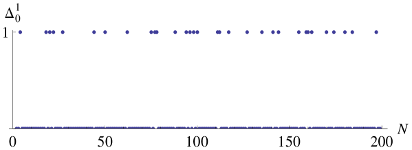
Figure 7: $N\mapsto\Delta_{0}^{1}(N)$. See text.

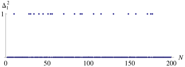
Figure 8: $N\mapsto\Delta_{1}^{2}(N)$. See text.

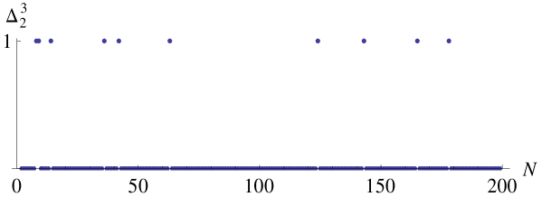
Figure 9: $N\mapsto\Delta_{2}^{3}(N)$. See text.

This concludes our data analysis section. We next present our theoretical results.

3 (Quasi-)rigorous upper bounds on $s_{*}$

While it may not be so easy to obtain a rigorous lower bound on $s_{*}$, it is relatively easy to find a rigorous upper bound on $s_{*}$ by studying the $s$-dependence of $\ddot{v}_{s}(3)$; and with the help of computer evaluations of $\ddot{v}_{s}(N)$ for $N\in\{3,4,5,6\}$ we easily obtained better, though only “quasi-rigorous,” upper bounds on $s_{*}$.

To study the $s$-dependence of $\ddot{v}_{s}(N)$ for $N\in\{3,4,5,6\}$ when $s>-2$, we need to know the minimizing $N$-point configurations for $N\in\{2,3,4,5,6,7\}$ if $-2\leq s<\infty$. We begin by summarizing what we know about these.

3.1 ${\omega}_{N}^{s}$ for $N\in\{2,3,4,5,6,7\}$ and $s\in(-2,\infty)$

Below we list the four rigorously known optimizers $\omega_{N}^{s}$, $N\in\{2,3,4,6\}$, together with the partly rigorously known but mostly computer-generated putative optimizers $\omega_{5}^{s}$ and $\omega_{7}^{s}$ for $s\in(-2,\infty)$. Note that for $N\in\{2,3,4,6\}$ each optimizer $\omega_{N}^{s}$ is independent of $s\in(-2,\infty)$, while the (putative) optimizers $\omega_{5}^{s}$ and $\omega_{7}^{s}$ display a non-trivial dependence on $s\in(-2,\infty)$:

$$\omega_{2}^{s} : \quad\mbox{two antipodal points}\hskip 55.0pts\in(-2,\infty);$$ (24)

$$\omega_{3}^{s} : \quad\mbox{equatorial equilateral triangle}\hskip 10.0pts\in(-2,\infty);$$ (25)

$$\omega_{4}^{s} : \quad\mbox{regular tetrahedron}\hskip 62.0pts\in(-2,\infty);$$ (26)

$$\omega_{5}^{s} : \begin{cases}\mbox{triangular bi-pyramid}&\quad\hskip 20.0pts\in(-2,15.04807...],\\ \mbox{square pyramid $(f=1)$}&\quad\hskip 20.0pts\in[15.04807...,\infty);\end{cases}$$ (27)

$$\omega_{6}^{s} : \quad\mbox{regular octahedron}\hskip 65.0pts\in(-2,\infty);$$ (28)

$$\omega_{7}^{s} : \begin{cases}C_{2}(1^{1}2^{3})(f=5)&\quad\hskip 24.0pts\in(-2,0],\\ \mbox{pentagonal bi-pyramid}&\quad\hskip 24.0pts\in[0,2],\\ C_{2}(1^{1}2^{3})(f=5)&\quad\hskip 24.0pts\in[2,5],\\ C_{2v}(1^{1}4^{1}2^{1})(f=3)&\quad\hskip 24.0pts\in[5,5.5979...],\\ C_{3v}(1^{1}3^{2})(f=2)&\quad\hskip 24.0pts\in[5.5979...,\infty).\end{cases}$$ (29)

In the above we use the Schönflies point group notation; $f$ is the number of degrees of freedom of the configuration; e.g., for the square pyramid at $N=5$ the height varies with $s$. The configurations for $N\in\{5,7\}$ are taken from [MKS77] for $s\geq 1$, and from [BeHa77] for $s=-1$. As to the $C_{2}$-symmetric $N=7$ configuration at $s=-1$, we quote from [BeHa77]: “It consists of two points almost antipodal and the remaining five points sprinkled around an equatorial band.” This suggested to us that this configuration belongs to a family which bifurcates off of the pentagonal bi-pyramid, which we then computed numerically ourselves to happen at $s=0$. Moreover, by the nearly complete degeneracy of the $s=-2$ problem, this family of configurations will have another bifurcation point at $s=-2$. Intriguingly, geometrically this is the “same” $C_{2}$ family of configurations which was discovered by [MKS77] to bifurcate off of the pentagonal bi-pyramid at $s=2$ and to merge with the $C_{2v}$ configuration at $s=5$ (note, though, that [MKS77] did not carry out a complete bifurcation analysis); yet, presumably the five degrees of freedom in the family will be differently optimized in each family, in the sense that for most (if not all) $s\in(-2,0)$ there is no $s\in(2,5)$ with the same configuration.

3.2 Explicit maps $s\mapsto{v}_{s}(N)$ for $N\in\{2,3,4,5,6,7\}$

Based on the table shown in Subsection 3.1 we computed explicit expressions for $v_{s}(N)$ in all situations where we did not have to numerically optimize any of the degrees of freedom. Thus, for $N\in\{2,3,4,6\}$ and $s\in(-2,\infty)$ one has

$${v}_{s}(2) =\textstyle\frac{1}{s}\left(\big{(}\frac{1}{2}\big{)}^{s}-1\right),$$ (30)

$${v}_{s}(3) =\textstyle\frac{1}{s}\left(\big{(}\frac{1}{3}\big{)}^{\frac{s}{2}}-1\right),$$ (31)

$${v}_{s}(4) =\textstyle\frac{1}{s}\left(\big{(}\frac{3}{8}\big{)}^{\frac{s}{2}}-1\right),$$ (32)

and

$${v}_{s}(6)=\textstyle\frac{1}{s}\left(\frac{1}{5}\big{(}\frac{1}{2}\big{)}^{s}+\frac{4}{5}\big{(}\frac{1}{2}\big{)}^{\frac{s}{2}}-1\right),$$ (33)

while for $v_{s}(5)$ an explicit expression is available for $s\in(-2,15.04807...]$, viz.

$${v}_{s}(5)=\textstyle\frac{1}{s}\left(\frac{1}{10}\big{(}\frac{1}{2}\big{)}^{s}+\frac{3}{10}\big{(}\frac{1}{3}\big{)}^{\frac{s}{2}}+\frac{3}{5}\big{(}\frac{1}{2}\big{)}^{\frac{s}{2}}-1\right),$$ (34)

and for $v_{s}(7)$ the following expression is valid for $s\in(0,2)$:

$${v}_{s}(7)=\textstyle\frac{1}{s}\left(\frac{1}{21}\big{(}\frac{1}{2}\big{)}^{s}+\frac{5}{21}\!\left(\!\left(2\sin\frac{2\pi}{5}\right)^{-s}+\left(2\sin\frac{\pi}{5}\right)^{-s}\right)+\frac{10}{21}\big{(}\frac{1}{2}\big{)}^{\frac{s}{2}}-1\right).$$ (35)

3.3 Bounds on $s_{*}$ from $s\mapsto\ddot{v}_{s}(3)$ for $s\in(-2,\infty)$

Only for $N=3$ can we compute $\ddot{v}_{s}(N)$ for all $s>-2$, viz.

$$\ddot{v}_{s}(3)=\textstyle\frac{1}{s}\left(\big{(}\frac{1}{2}\big{)}^{s}+\big{(}\frac{3}{8}\big{)}^{\frac{s}{2}}-2\big{(}\frac{1}{3}\big{)}^{\frac{s}{2}}\right).$$ (36)

The elementary function $s\mapsto\ddot{v}_{s}(3)$ is sufficiently simple to allow a thoroughly rigorous discussion. Thus, inserting $s=-2$ we obtain $\ddot{v}_{-2}(3)=-1/3$, but we already knew that any function $s\mapsto\ddot{v}_{s}(N)$ had to be strictly negative at $s=-2$. On the other hand, rewriting $\ddot{v}_{s}(3)$ as

$$\ddot{v}_{s}(3)=\textstyle\frac{1}{s}\big{(}\frac{3}{8}\big{)}^{\frac{s}{2}}\left(1-\big{(}\frac{8}{9}\big{)}^{\frac{s}{2}}\left(1-\big{(}\frac{3}{4}\big{)}^{\frac{s}{2}}\right)\right),$$ (37)

we can extract the large-$s$ asymptotic behavior $\ddot{v}_{s}(3)\asymp\frac{1}{s}\Big{(}\frac{3}{8}\Big{)}^{\frac{s}{2}}>0$. As a continuous function, $\ddot{v}_{s}(3)$ therefore has to have an odd number of zeros in $(-2,\infty)$. Let $s_{1}^{(3)}$ denote the smallest zero of $\ddot{v}_{s}(3)$ in $(-2,\infty)$. Then $s_{*}\leq s_{1}^{(3)}$, rigorously.

Of course, the bound $s_{*}\leq s_{1}^{(3)}$ is not explicit. An explicit upper bound is obtained by inserting $s=10$ into (36), or (37), which yields the strictly positive (tiny) value $\ddot{v}_{10}(3)=1289/79626240$. Thus we have rigorously proved:

Proposition 3.

The critical $s_{*}$ satisfies the upper bound $s_{*}\leq s_{1}^{(3)}<10$.

With a little extra effort one can show that $\ddot{v}_{s}(3)$ has exactly one zero in $(-2,\infty)$. Namely, starting at $s=-2$ with a strictly negative value, $\ddot{v}_{s}(3)$ then increases monotonically to a single — strictly positive — maximum, after which it decays monotonically to zero as $s\to\infty$. We illustrate this behavior with a mathematica plot of $s\mapsto\ddot{v}_{s}(3)$, see Fig. 10.

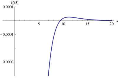
Figure 10: Behavior of $\ddot{v}_{s}(3)$ as a function of $s$.

Numerically we get $s_{1}^{(3)}\approx 9.4$, so that our explicit upper bound on $s_{*}$ is not much worse than this numerically computed bound on $s_{*}$.

The bound stated in Proposition 3 is the only upper bound on $s_{*}$ which we were able to establish with complete rigor by analyzing explicitly known finite-$N$ optimizers. Quantitatively this bound is lousy. In particular, as mentioned in the introduction, Hardin and Saff [HaSa05] rigorously showed that $N\mapsto{v}_{s}(N)$ is asymptotically, for large $N$, strictly convex when $s>4$, which implies that $s_{*}\leq 4$.

In the ensuing subsections we will obtain several (much) better upper bounds, alas aided by a computer. Some of these are stated as (conditional) propositions, which includes Proposition 2.

3.4 Bounds on $s_{*}$ via $s\mapsto\ddot{v}_{s}(4)$, $-2<s\leq 15.048...$

For $N=4$ we can explicitly compute $\ddot{v}_{s}(N)$ when $-2<s\leq 15.04807...$, namely:

$$\ddot{v}_{s}(4) =\textstyle\frac{1}{s}\left(\frac{1}{10}\big{(}\frac{1}{2}\big{)}^{s}+\frac{13}{10}\big{(}\frac{1}{3}\big{)}^{\frac{s}{2}}+\frac{3}{5}\big{(}\frac{1}{2}\big{)}^{\frac{s}{2}}-2\big{(}\frac{3}{8}\big{)}^{\frac{s}{2}}\right).$$ (38)

The $s$-dependence of this elementary function is also simple enough to allow a thoroughly rigorous discussion, which reveals the following. Thus, $\ddot{v}_{-2}(4)$ is strictly negative, again as we know already it must. Also the large-$s$ asymptotics of r.h.s.(38) can be worked out immediately, r.h.s.(38)$\,\asymp\frac{1}{s}\frac{3}{5}\big{(}\frac{1}{2}\big{)}^{\frac{s}{2}}>0$, yielding the information that r.h.s.(38) has an odd number of zeros in $(-2,\infty)$. However, since the validity of the expression (38) is restricted to $s\in(-2,15.04807...]$, the asymptotic result does not yield relevant information which — in concert with the strict negativity of $\ddot{v}_{-2}(4)$ — would allow us to draw any conclusions about $s\mapsto\ddot{v}_{s}(4)$ in $s\in(-2,15.04807...]$. Instead we need to take a closer look.

Inserting $s=2$, we easily find $\ddot{v}_{2}(4)=\frac{41}{120}>0$. As a continuous function, $\ddot{v}_{s}(4)$ therefore has to have an odd number of zeros in $(-2,2)$. Let $s_{1}^{(4)}$ denote the smallest zero of $\ddot{v}_{s}(4)$ in $(-2,2)$. Then $s_{1}^{(4)}$ is a (quasi-)rigorous upper bound on $s_{*}$. Also the bound $s_{*}\leq s_{1}^{(4)}$ is not explicit, but $s_{1}^{(4)}<2$ gives the explicit (quasi-)rigorous upper bound $s_{*}<2$ which improves over $s_{*}<10$, and also over $s_{*}\leq 4$ from the asymptotic analysis [HaSa05].

Also, with the aid of maple (or such) the explicit quasi-rigorous upper bound can be improved to $s_{*}<1$, for numerically ${\ddot{v}_{1}(4)=0.0000745467...>0}$ (in remarkable agreement with the numerical data extracted from the computer experiments), so that $s_{1}^{(4)}<1$. In fact, this can also be made quasi-rigorous.

Proposition 4.

The critical $s_{*}$ satisfies the upper bound $s_{*}<1$ as

$$\ddot{v}_{1}(4)=\textstyle\frac{1}{20}+\frac{13}{10}\big{(}\frac{1}{3}\big{)}^{\frac{1}{2}}+\frac{3}{5}\big{(}\frac{1}{2}\big{)}^{\frac{1}{2}}-\big{(}\frac{3}{2}\big{)}^{\frac{1}{2}}>0.$$ (39)

Proof.

First, we derive a sufficiently tight lower bound of $(1-x)^{1/2}$ in terms of a polynomial that gives a rational number if $x$ is rational. (The usual Taylor polynomial with Lagrange remainder term does not provide good enough bounds.) Using the binomial formula, Pochhammer symbols, and Gauss hypergeometric functions, we get for every positive integer $K$

$$\left(1-x\right)^{1/2} =\sum_{k=0}^{\infty}\binom{1/2}{k}(-x)^{k}=\sum_{k=0}^{K-1}\frac{{\left(-1/2\right)_{k}}}{k!}x^{k}+\sum_{k=K}^{\infty}\frac{{\left(-1/2\right)_{k}}}{k!}x^{k}$$

$$=\sum_{k=0}^{K-1}\frac{{\left(-1/2\right)_{k}}}{k!}x^{k}+\frac{{\left(-1/2\right)_{K}}}{K!}x^{K}{\sideset{{}_{2}}{{}_{1}}{\operatorname{F}}\!\left(\begin{subarray}{c}\displaystyle K-1/2,1\\ \displaystyle K+1\end{subarray};x\right)}.$$

Since ${\left(-1/2\right)_{K}}=\Gamma(K-1/2)/\Gamma(-1/2)<0$, and since the Gauss hypergeometric function is strictly increasing in $x$ on $[0,1]$, assuming the value $2K$ at $x=1$ (cf. DLMF Eq. 15.4.20), we arrive at

$$\left(1-x\right)^{1/2}>\sum_{k=0}^{K-1}\frac{{\left(-1/2\right)_{k}}}{k!}x^{k}-\frac{{\left(1/2\right)_{K-1}}}{(K-1)!}x^{K}\qquad\text{for $0<x<1$.}$$

Thus, we estimate

$$\left(\frac{1}{3}\right)^{1/2} =\left(1-\frac{2}{3}\right)^{1/2}>\sum_{k=0}^{K-1}\frac{{\left(-1/2\right)_{k}}}{k!}\left(\frac{2}{3}\right)^{k}-\frac{{\left(1/2\right)_{K-1}}}{(K-1)!}\left(\frac{2}{3}\right)^{K},$$

$$\left(\frac{1}{2}\right)^{1/2} =\left(1-\frac{1}{2}\right)^{1/2}>\sum_{k=0}^{K-1}\frac{{\left(-1/2\right)_{k}}}{k!}\left(\frac{1}{2}\right)^{k}-\frac{{\left(1/2\right)_{K-1}}}{(K-1)!}\left(\frac{1}{2}\right)^{K}$$

for any positive integer $K$, whereas for even positive integers $K$

$$\left(\frac{3}{2}\right)^{1/2}=\left(1+\frac{1}{2}\right)^{1/2}<1+\sum_{k=1}^{K-1}\frac{{\left(-1/2\right)_{k}}}{k!}(-1)^{k}\left(\frac{1}{2}\right)^{k},$$

because the binomial expansion of $(1+x)^{1/2}-1$ is an alternating series.

Let $K=20$. Combining everything, we get

$$\ddot{v}_{1}(4) =\frac{1}{20}+\frac{13}{10}\left(\frac{1}{3}\right)^{1/2}+\frac{3}{5}\left(\frac{1}{2}\right)^{1/2}-\left(\frac{3}{2}\right)^{1/2}$$

$$>\frac{5764409437417341241721}{209374412387531441339105280}>0.$$

For the computation of the rational bounds one can use, e.g., mathematica. Hence, by the definition of $s_{*}$ we obtain the desired result. ∎

With some extra energy one should be able to make the above bounds totally rigorous, but this would require to prove that the triangular bi-pyramid is the $N=5$ optimizer for $s\in[0,2]$, say.

For the sake of completeness, in Fig. 11 we display a numerical plot of $s\mapsto\ddot{v}_{s}(4)$ for $s\in(-2,15.04807...]$.

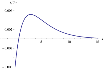
Figure 11: Behavior of $\ddot{v}_{s}(4)$ as a function of $s$ for $s\in(-2,15.04807...]$.

3.5 Bounds on $s_{*}$ from $s\mapsto\ddot{v}_{s}(6)$ for $0<s<2$

We now give a computer-assisted proof of Proposition 2.

Proof.

For $0<s<2$ we find

$$\ddot{v}_{s}(6)=\textstyle\frac{1}{s}\!\left(\!\frac{5}{21}\!\left(\!\left(2\sin\frac{2\pi}{5}\right)^{-s}\!+\!\left(2\sin\frac{\pi}{5}\right)^{-s}\right)\!+\!\frac{3}{10}\big{(}\frac{1}{3}\big{)}^{\frac{s}{2}}\!-\!\frac{11}{21}\big{(}\frac{1}{2}\big{)}^{\frac{s}{2}}\!-\!\frac{53}{210}\big{(}\frac{1}{2}\big{)}^{s}\right)\!.\!\!$$ (40)

The $s$-dependence of this elementary function is less simple. Moreover, the bifurcation of the $N=7$ minimizers at $s=0$ is known to us only through our numerical bifurcation analysis, so that it seems prudent for now to be satisfied with a computer-assisted evaluation. Fig. 12 shows a numerical rendering of r.h.s.(40).

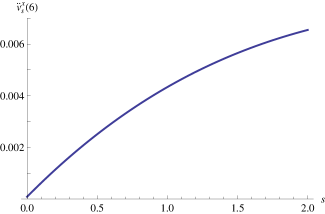
Figure 12: Graph of $\ddot{v}_{s}(6)$ for $s\in(0,2)$.

Numerically, $\lim_{s\to 0}\ddot{v}_{s}(6)=0.000084098...>0$, and since $\ddot{v}_{-2}(6)<0$, we conclude that the continuous map $s\mapsto\ddot{v}_{s}(6)$ has an odd number of zeros in $(-2,0)$. Let $s_{1}^{(6)}$ be the smallest one. Then $s_{*}\leq s_{1}^{(6)}<0$. This proves Proposition 2. ∎

3.6 Remarks on $s\mapsto\ddot{v}_{s}(12)$ for $-2<s<2$

Fig.s 3 and 4 suggest that the $N=6$ peak increases more rapidly with $s$ than the $N=12$ peak when $s$ runs from $0$ to $1$. Since the $N=12$ peak appears to be the highest peak for $s=0$ while the $N=6$ peak is barely above zero then, we suspect that by lowering $s$ below $0$ the $N=12$ peak will vanish at a lower $s$-value than the $N=6$ peak, so that the first zero of $s\mapsto\ddot{v}_{s}(12)$ will yield a better upper bound on $s_{*}$ than the one we have found with $N=6$.

Unfortunately, to evaluate $s\mapsto\ddot{v}_{s}(12)$ one needs to know the optimal configurations for $N\in\{11,13\}$. We are planning a computer-assisted evaluation of $s\mapsto\ddot{v}_{s}(12)$, which seems to be the best one can do right now.

4 Rigorous bounds on $\ddot{v}_{s}(N)$

4.1 Generic $\mathcal{O}(N^{-2})$ upper bounds on $\ddot{v}_{s}(N)$ for $s<0$

We now derive the following positive $\mathcal{O}(N^{-2})$ upper bound on $\ddot{v}_{s}(N)$ for $s<0$.

Proposition 5.

For $s<0$ the second derivative of ${v}_{s}(N)$ is bounded above by

$$\ddot{v}_{s}(N)\leq-\frac{2}{(N+1)N}\left(v_{s}(N-1)+\frac{1}{s}\right).$$ (41)

Proof.

We rewrite

$$2v_{s}(N)=(1+\delta)v_{s}(N)+(1-\delta)v_{s}(N),$$ (42)

where $\delta=2/(N+1)$. Next, since

$$v_{s}(N)=\langle V_{s}\rangle(\omega_{N}^{s}),$$

using (3) we now rewrite (42) further as

$$2v_{s}(N) =\left(1+\delta\right)\frac{2}{N(N-1)}\mathop{\sum\sum}_{1\leq i<j\leq N-1}V_{s}(|{\boldsymbol{{q}}}_{i}^{s}-{\boldsymbol{{q}}}_{j}^{s}|)$$

$$\phantom{=}+\left(1+\delta\right)\frac{2}{N(N-1)}\sum_{1\leq i\leq N-1}V_{s}(|{\boldsymbol{{q}}}_{i}^{s}-{\boldsymbol{{q}}}_{N}^{s}|)$$

$$\phantom{=}+\left(1-\delta\right)\frac{2}{N(N-1)}\mathop{\sum\sum}_{1\leq i<j\leq N}V_{s}(|{\boldsymbol{{q}}}_{i}^{s}-{\boldsymbol{{q}}}_{j}^{s}|),$$

and so, using that $\delta=2/(N+1)$,

$$\begin{split}2v_{s}(N)&=\frac{2(N+3)}{(N+1)N(N-1)}\mathop{\sum\sum}_{1\leq i<j\leq N-1}V_{s}(|{\boldsymbol{{q}}}_{i}^{s}-{\boldsymbol{{q}}}_{j}^{s}|)\\ &\phantom{=}+\frac{2(N+3)}{(N+1)N(N-1)}\sum_{1\leq i\leq N-1}V_{s}(|{\boldsymbol{{q}}}_{i}^{s}-{\boldsymbol{{q}}}_{N}^{s}|)\\ &\phantom{=}+\frac{2}{(N+1)N}\mathop{\sum\sum}_{1\leq i<j\leq N}V_{s}(|{\boldsymbol{{q}}}_{i}^{s}-{\boldsymbol{{q}}}_{j}^{s}|).\end{split}$$ (43)

For the term in the second line we use that $N+3=(N-1)+4$ and rewrite

$$\frac{2(N+3)}{(N+1)N(N-1)}=\frac{2}{(N+1)N}+\frac{8}{(N+1)N(N-1)}.$$ (44)

In the single sum receiving the factor $2/(N+1)N$ we now rename the point ${\boldsymbol{{q}}}_{N}^{s}$ into ${\boldsymbol{{q}}}_{N+1}^{\prime}$ and pool this single sum together with the double sum in the last line in (43), obtaining

$$\sum_{1\leq i\leq N-1}V_{s}(|{\boldsymbol{{q}}}_{i}^{s}-{\boldsymbol{{q}}}_{N+1}^{\prime}|)+\mathop{\sum\sum}_{1\leq i<j\leq N}V_{s}(|{\boldsymbol{{q}}}_{i}^{s}-{\boldsymbol{{q}}}_{j}^{s}|)=\frac{1}{s}+\mathop{\sum\sum}_{1\leq i<j\leq N+1}V_{s}(|{\boldsymbol{{q}}}_{i}^{\prime}-{\boldsymbol{{q}}}_{j}^{\prime}|),$$ (45)

where ${\boldsymbol{{q}}}_{k}^{\prime}={\boldsymbol{{q}}}_{k}^{s}$ for $1\leq k\leq N$ and ${\boldsymbol{{q}}}_{N+1}^{\prime}={\boldsymbol{{q}}}_{N}^{s}$, and where we used that $V_{s}(0)=-\frac{1}{s}$ for $s<0$; now multiplying by $2\big{/}(N+1)N$ and recalling (3) yields

$$\begin{split}&\frac{2}{(N+1)N}\left(\sum_{1\leq i\leq N-1}V_{s}(|{\boldsymbol{{q}}}_{i}^{s}-{\boldsymbol{{q}}}_{N+1}^{\prime}|)+\mathop{\sum\sum}_{1\leq i<j\leq N}V_{s}(|{\boldsymbol{{q}}}_{i}^{s}-{\boldsymbol{{q}}}_{j}^{s}|)\right)\\ &\phantom{equals}=\frac{2}{(N+1)N}\,\frac{1}{s}+\langle V_{s}\rangle(\omega_{N+1}^{\prime}),\end{split}$$ (46)

where $\omega_{N+1}^{\prime}=\{{\boldsymbol{{q}}}_{1}^{\prime},...,{\boldsymbol{{q}}}_{N+1}^{\prime}\}$.

For the remaining single sum, with factor $8\big{/}(N+1)N(N-1)$, we note that without loss of generality we may assume that

$$\sum_{1\leq i\leq N-1}V_{s}(|{\boldsymbol{{q}}}_{i}^{s}-{\boldsymbol{{q}}}_{N}^{s}|)\geq\sum_{\begin{subarray}{c}1\leq i\leq N,\\ i\neq j\end{subarray}}V_{s}(|{\boldsymbol{{q}}}_{i}^{s}-{\boldsymbol{{q}}}_{j}^{s}|),\qquad\forall j=1,\dots,N;$$

but then

$$\frac{1}{N-1}\sum_{1\leq i\leq N-1}V_{s}(|{\boldsymbol{{q}}}_{i}^{s}-{\boldsymbol{{q}}}_{N}^{s}|)\geq\frac{2}{N(N-1)}\mathop{\sum\sum}_{1\leq i<j\leq N}V_{s}(|{\boldsymbol{{q}}}_{i}^{s}-{\boldsymbol{{q}}}_{j}^{s}|),$$

and therefore also

$$\frac{1}{N-1}\sum_{1\leq i\leq N-1}V_{s}(|{\boldsymbol{{q}}}_{i}^{s}-{\boldsymbol{{q}}}_{N}^{s}|)\geq\frac{2}{(N-1)(N-2)}\mathop{\sum\sum}_{1\leq i<j\leq N-1}V_{s}(|{\boldsymbol{{q}}}_{i}^{s}-{\boldsymbol{{q}}}_{j}^{s}|).$$ (47)

This estimate of the single sum from the middle line of (43) in terms of the double sum in the first line of (43) gives us

$$\frac{2(N+3)}{(N+1)N(N-1)}\mathop{\sum\sum}_{1\leq i<j\leq N-1}V_{s}(|{\boldsymbol{{q}}}_{i}^{s}-{\boldsymbol{{q}}}_{j}^{s}|)$$

$$\phantom{equals=}+\frac{8}{(N+1)N(N-1)}\sum_{1\leq i\leq N-1}V_{s}(|{\boldsymbol{{q}}}_{i}^{s}-{\boldsymbol{{q}}}_{N}^{s}|)$$

$$\phantom{equals}\geq\frac{(N+3)(N-2)+8}{(N+1)N}\,\frac{2}{(N-1)(N-2)}\mathop{\sum\sum}_{1\leq i<j\leq N-1}V_{s}(|{\boldsymbol{{q}}}_{i}^{s}-{\boldsymbol{{q}}}_{j}^{s}|)$$

$$\phantom{equals}=\left(1+\frac{2}{(N+1)N}\right)\langle V_{s}\rangle(\omega^{s}_{N}{\!\setminus\!}\{{\boldsymbol{{q}}}^{s}_{N}\}).$$

In total, we therefore have the estimate

$$2v_{s}(N)\geq\frac{2}{(N+1)N}\,\frac{1}{s}+\langle V_{s}\rangle(\omega_{N+1}^{\prime})+\left(1+\frac{2}{(N+1)N}\right)\langle V_{s}\rangle(\omega^{s}_{N}{\!\setminus\!}\{{\boldsymbol{{q}}}^{s}_{N}\}),$$ (48)

which can be estimated again with the help of (4) to get

$$2v_{s}(N)\geq{{\frac{2}{(N+1)N}}}\,\frac{1}{s}+v_{s}({N+1})+\left(1+{{\frac{2}{(N+1)N}}}\right)v_{s}({N-1}).$$ (49)

Regrouping terms in (49) we get

$$v_{s}(N-1)-2v_{s}(N)+v_{s}(N+1)\leq-{{\frac{2}{(N+1)N}}}\left(\frac{1}{s}+v_{s}({N-1})\right).$$ (50)

The proof is complete. ∎

Remark 4.

Step (45) requires $V_{s}(0)<\infty$, which is true only for $s<0$.

Remark 5.

For $s<0$ we have $\frac{1}{s}+v_{s}({N-1})<0$ so that r.h.s.(50) $>0$.

Remark 6.

For the special value $s=-2$ we have the exact result (109), and a direct computation shows that $\ddot{v}_{-2}(N)=-2/(N-1)^{3}<0$. Therefore, at least for $s=-2$, the upper estimate is not optimal.

Also, for $s<-2$ and even $N$ we have the exact result (110), which converges to $v_{-2}(N)$ when taking the limit $s\uparrow-2$ of (110). Again, a simple computation shows that $\ddot{v}_{s}(N)<0$ for $s<-2$ and $N$ even. Modulo confirming that the situation doesn’t change when $N$ is odd, the upper bound on $\ddot{v}_{s}(N)$ for $s<0$ would be non-optimal for all $s\leq-2$.

Remark 7.

The ${1}/{s}$ at r.h.s.(50) is a consequence of our definition of $V_{s}(r)$. By working instead with $\widetilde{V}_{s}(r)=r^{-s}/s$, the $1/s$ term will not show up in (45) and (LABEL:MIDDLEsumDOUBLEsumMERGErewrite) and hence be absent in (50), which would read

$$\widetilde{v}_{s}(N-1)-2\,\widetilde{v}_{s}(N)+\widetilde{v}_{s}(N+1)\leq-{{\frac{2}{(N+1)N}}}\,\widetilde{v}_{s}({N-1}).$$ (51)

Note that indeed, the $1/s$ at r.h.s.(50) cancels against the $-1/s$ implicit in $v_{s}({N-1})$, and l.h.s.(50) is invariant under the change $V_{s}(r)\to\widetilde{V}_{s}(r)$ so that our (50) is quantitatively identical to (51).

Remark 8.

If one could improve the factor 2 at r.h.s.(47) into a $3/2$, this would prove concavity. However, the inequality (47) turns out to be sometimes an equality (e.g. when $s=-1$ and $N=3$ or $N=4$). Also (48), rewritten as

$$\begin{split}v_{s}(N-1)-2v_{s}(N)+v_{s}(N+1)&\leq v_{s}(N+1)-\langle V_{s}\rangle(\omega_{N+1}^{\prime})\\ &\phantom{=}+v_{s}(N-1)-\langle V_{s}\rangle(\omega^{s}_{N}{\!\setminus\!}\{{\boldsymbol{{q}}}^{s}_{N}\})\\ &\phantom{=}-\frac{2}{(N+1)N}\left(\frac{1}{s}+\langle V_{s}\rangle(\omega^{s}_{N}{\!\setminus\!}\{{\boldsymbol{{q}}}^{s}_{N}\})\right),\end{split}$$ (52)

is still sometimes an equality! For instance, take $s=-1$, then $v_{-1}(2)=1-2$ and $v_{-1}(3)=1-\sqrt{3}$ and $v_{-1}(4)=1-2\sqrt{2/3}$, so for $N=3$ then $\ddot{v}_{-1}(3)=v_{-1}(2)-2v_{s}(3)+v_{s}(4)=2(-1+\sqrt{3}-\sqrt{2/3})=-0.168891546...$, and the exact evaluation of r.h.s.(52) yields the same answer.

Remark 9.

The only true inequality is in the step from (48) to (49). Thus, to prove concavity at least for some $s$-values one has to improve this estimate.

We have checked that for $s=-1$ and $N=3$ the sum of the second line at r.h.s.(52) alone does not dominate the term in the third line; namely the sum of these two terms is $(7/6)\sqrt{3}-2>0$. Also, the term in the first line at r.h.s.(52) alone does not dominate the one in the third line in this case; namely, their sum equals $\sqrt{3}(1-2\sqrt{2}/3)>0$, too. Therefore, to prove concavity (for some negative $s$-values, say $s\leq-1$), one will need to prove that the first two lines at the r.h.s.(52) together are more negative than the last line is positive, at least for a certain range of negative $s$-values.

4.2 Point-energies: better $\mathcal{O}(N^{-2})$ bounds on $\!\ddot{v}_{s}(N),\,s<0$

So far our analysis has only used the concept of an “energy of a configuration of $N$ points,” which is based on the interpretation of $V_{s}(|{\boldsymbol{{q}}}-{\boldsymbol{{q}}}^{\prime}|)$ as a pair-energy. We now bring in the well-known concept of an “energy of an individual point,” or point-energy for short, which is based on the interpretation of $V_{s}(|{\boldsymbol{{q}}}-{\boldsymbol{{q}}}^{\prime}|)$ as the (potential) energy of a particle located at ${\boldsymbol{{q}}}$ in the potential field of a particle at ${\boldsymbol{{q}}}^{\prime}$, a notion which is clearly reflexive.

We recall that every (unlabeled) $N$-point configuration $\omega_{N}$ on $\mathbb{S}^{2}$ can be assigned a unique compatible family of normalized, so-called empirical $n$-point measures, with $1\leq n\leq N$, and vice versa. For instance, with the help of any labeling, the first two of these can be written as

$$\underline{\Delta}^{(1)}_{\omega_{N}}(d{\boldsymbol{{q}}})={{\frac{1}{N}}}\sum_{1\leq j\leq N}\delta_{{\boldsymbol{{q}}}_{j}}(d{\boldsymbol{{q}}}),$$ (53)

$$\underline{\Delta}^{(2)}_{\omega_{N}}(d{\boldsymbol{{q}}}d{\boldsymbol{{q}}}^{\prime})={{\frac{2}{N(N-1)}}}\sum\!\sum_{\hskip-19.91684pt1\leq j<k\leq N}\delta_{{\boldsymbol{{q}}}_{j}}(d{\boldsymbol{{q}}})\delta_{{\boldsymbol{{q}}}_{k}}(d{\boldsymbol{{q}}}^{\prime}),$$ (54)

and analogously one writes the empirical measures of higher order $n=3,...,N$; here, with a mild abuse of notation, $\delta_{{\boldsymbol{{q}}}_{j}}(d{\boldsymbol{{q}}})$ denotes the Dirac measure on $\mathbb{S}^{2}$ concentrated at ${\boldsymbol{{q}}}_{j}$, i.e. for any Borel subset $\Lambda$ of $\mathbb{S}^{2}$ we have $\int_{\Lambda}\delta_{{\boldsymbol{{q}}}_{j}}(d{\boldsymbol{{q}}})=0$ if ${\boldsymbol{{q}}}_{j}\not\in\Lambda$, and $\int_{\Lambda}\delta_{{\boldsymbol{{q}}}_{j}}(d{\boldsymbol{{q}}})=1$ if ${\boldsymbol{{q}}}_{j}\in\Lambda$. With the help of $\underline{\Delta}^{(2)}_{\omega_{N}}$ we can rewrite the average standardized Riesz pair-energy of an $N$-point configuration $\omega_{N}$ as

$$\langle V_{s}\rangle(\omega_{N})={\int\!\!\!\!\int}_{\mathbb{S}^{2}\times\mathbb{S}^{2}}V_{s}\left(\left|{\boldsymbol{{q}}}-{\boldsymbol{{q}}}^{\prime}\right|\right)\underline{\Delta}^{(2)}_{\omega_{N}}(d{\boldsymbol{{q}}}d{\boldsymbol{{q}}}^{\prime}).$$ (55)

Moreover, with the help of $\underline{\Delta}^{(1)}_{\omega_{N}}$ we can now associate with each $N$-point configuration $\omega_{N}$ a standardized Riesz $s$-potential function on $\mathbb{S}^{2}$, given by

$$\big{(}V_{s}\star\underline{\Delta}^{(1)}_{\omega_{N}}\big{)}({\boldsymbol{{q}}})\equiv\int_{\mathbb{S}^{2}}V_{s}\left(\left|{\boldsymbol{{q}}}-{\boldsymbol{{q}}}^{\prime}\right|\right)\underline{\Delta}^{(1)}_{\omega_{N}}(d{\boldsymbol{{q}}}^{\prime}),\qquad{\boldsymbol{{q}}}\in\mathbb{S}^{2},\quad s<0.$$ (56)

Remark 10.

Since $s<0$, the potential function (56) is well-defined and finite on all of $\mathbb{S}^{2}$ because $V_{s}:\mathbb{R}_{+}\to\mathbb{R}$ is continuous for $s<0$. Of course, provided one restricts ${\boldsymbol{{q}}}$ to $\mathbb{S}^{2}\!\setminus\!\omega_{N}$, one can also extend (56) continuously to the regime $s\geq 0$. Moreover, when $s\in[0,2)$ the function ${\boldsymbol{{q}}}^{\prime}\mapsto V_{s}\left(\left|{\boldsymbol{{q}}}-{\boldsymbol{{q}}}^{\prime}\right|\right)$ is weakly lower semi-continuous (i.e. $V_{s}$ is the pointwise limit of an increasing sequence of continuous functions), and therefore the potential function (56) is well-defined (in the sense that it may be positive infinite for certain ${\boldsymbol{{q}}}$) also for $N\to\infty$, whenever $\underline{\Delta}^{(1)}_{\omega_{N}}(d{\boldsymbol{{q}}}^{\prime})\rightharpoonup\mu(d{\boldsymbol{{q}}}^{\prime})$ in the weak^∗ sense, where $\mu(d{\boldsymbol{{q}}}^{\prime})$ is a regular Borel measure on $\mathbb{S}^{2}$. Note that $\big{(}V_{s}\star\mu\big{)}({\boldsymbol{{q}}})\leq\liminf\big{(}V_{s}\star\underline{\Delta}^{(1)}_{\omega_{N}}\big{)}({\boldsymbol{{q}}})$.

Of special interest to us are the standardized Riesz $s$-potentials of $N$-point configurations $\omega_{N}$ on $\mathbb{S}^{2}$ obtained from ${(N+1)}$-point configurations by removing any particular point — or rather: their analogues with $N$ replaced by $N-1$. Every $\omega_{N}$ defines a set of $N$ such ${(N-1)}$-point configurations. After introducing any convenient labeling of the points in $\omega_{N}$, this set of ${(N-1)}$-point configurations reads $\big{\{}{\omega_{N}{\!\setminus\!}\{{\boldsymbol{{q}}}_{\ell}\}}\big{\}}_{\ell=1}^{{}_{N}}$. For every ${(N-1)}$-point configuration there is a standardized Riesz $s$-potential function on $\mathbb{S}^{2}$, given by $\big{(}V_{s}\star\underline{\Delta}^{(1)}_{\omega_{N}{\!\setminus\!}\{{\boldsymbol{{q}}}_{\ell}\}}\big{)}({\boldsymbol{{q}}})$.

For every point ${\boldsymbol{{q}}}_{\ell}\in\omega_{N},\,\ell\in\{1,\dots,N\}$, its average standardized Riesz point-energy w.r.t. the reduced ${(N-1)}$-point configuration $\omega_{N}{\!\setminus\!}\{{\boldsymbol{{q}}}_{\ell}\}$ is simply the standardized Riesz $s$-potential of $\omega_{N}{\!\setminus\!}\{{\boldsymbol{{q}}}_{\ell}\}$ evaluated at ${\boldsymbol{{q}}}={\boldsymbol{{q}}}_{\ell}$, viz.

$$\frac{1}{N-1}\sum_{\begin{subarray}{c}1\leq j\leq N,\\ j\neq\ell\end{subarray}}V_{s}(|{\boldsymbol{{q}}}_{j}-{\boldsymbol{{q}}}_{\ell}|)=\big{(}V_{s}\star\underline{\Delta}^{(1)}_{\omega_{N}{\!\setminus\!}\{{\boldsymbol{{q}}}_{\ell}\}}\big{)}({\boldsymbol{{q}}}_{\ell}),\quad\ell=1,\dots,N.$$ (57)

Thus every $\omega_{N}$ defines a set of $N$ point-energies $\big{\{}\big{(}V_{s}\star\underline{\Delta}^{(1)}_{\omega_{N}{\!\setminus\!}\{{\boldsymbol{{q}}}_{\ell}\}}\big{)}({\boldsymbol{{q}}}_{\ell})\big{\}}_{\ell=1}^{{}_{N}}$. The average standardized Riesz pair-energy of $\omega_{N}$ is the mean of these:

$$\langle V_{s}\rangle(\omega_{N})=\frac{1}{N}\sum_{1\leq\ell\leq N}\big{(}V_{s}\star\underline{\Delta}^{(1)}_{\omega_{N}{\!\setminus\!}\{{\boldsymbol{{q}}}_{\ell}\}}\big{)}({\boldsymbol{{q}}}_{\ell}).$$ (58)

Remark 11.

Given a minimizing configuration $\omega_{N}^{s}$, it can easily be seen that

$$\big{(}V_{s}\star\underline{\Delta}^{(1)}_{\omega_{N}^{s}{\!\setminus\!}\{{\boldsymbol{{q}}}^{s}_{\ell}\}}\big{)}({\boldsymbol{{q}}})\geq\big{(}V_{s}\star\underline{\Delta}^{(1)}_{\omega_{N}^{s}{\!\setminus\!}\{{\boldsymbol{{q}}}^{s}_{\ell}\}}\big{)}({\boldsymbol{{q}}}^{s}_{\ell})\qquad\text{for all ${\boldsymbol{{q}}}\in\mathbb{S}^{2}$},$$ (59)

which simply says that each (generalized) unit point charge in a minimal-energy configuration occupies a point of minimal potential energy in the potential field generated by the remaining (generalized) unit point charges.

With the help of the so-defined potential functions and point energies, we are ready to prove Proposition 1, which improves the upper bound in Proposition 5 and also supplies a lower bound of the same type.

Proof.

(of Proposition 1) Using the definitions (3) and (57), for each $\ell=1,\dots,N$ we have

$$\langle V_{s}\rangle(\omega_{N})=\frac{N-2}{N}\,\langle V_{s}\rangle(\omega_{N}{\!\setminus\!}\{{\boldsymbol{{q}}}_{\ell}\})+\frac{2}{N}\big{(}V_{s}\star\underline{\Delta}^{(1)}_{\omega_{N}{\!\setminus\!}\{{\boldsymbol{{q}}}_{\ell}\}}\big{)}({\boldsymbol{{q}}}_{\ell}).$$ (60)

This will be our “master identity.”

First, averaging (60) over all ${\boldsymbol{{q}}}_{\ell}$, $\ell=1,\dots,N$, and recalling (58), gives

$$\langle V_{s}\rangle(\omega_{N})=\frac{1}{N}\sum_{1\leq\ell\leq N}\langle V_{s}\rangle(\omega_{N}{\!\setminus\!}\{{\boldsymbol{{q}}}_{\ell}\}).$$ (61)

Now replacing $\omega_{N}$ by $\omega_{N}^{s}=\{{\boldsymbol{{q}}}_{1}^{s},\dots,{\boldsymbol{{q}}}_{N}^{s}\}$, a minimizing $N$-point configuration, and using (4) for ${(N-1)}$-point configurations at the r.h.s., we recover the monotonicity relation

$$v_{s}(N)\geq v_{s}(N-1)\qquad\text{for all integers $N>2$;}$$ (62)

cf. [Lan72, Kie09a, Kie09b].

Second, replacing $\omega_{N}$ in (60) with $\omega_{N}\!\cup\!\{{\boldsymbol{{q}}}\}$, ${\boldsymbol{{q}}}\in\mathbb{S}^{2}$, and ${\boldsymbol{{q}}}_{\ell}$ by ${\boldsymbol{{q}}}$, yields

$$\langle V_{s}\rangle(\omega_{N}\!\cup\!\{{\boldsymbol{{q}}}\})=\frac{N-1}{N+1}\langle V_{s}\rangle(\omega_{N})+\frac{2}{(N+1)}\big{(}V_{s}\star\underline{\Delta}^{(1)}_{\omega_{N}}\big{)}({\boldsymbol{{q}}}),$$

or, equivalently,

$$\langle V_{s}\rangle(\omega_{N})=\frac{N+1}{N-1}\langle V_{s}\rangle(\omega_{N}\!\cup\!\{{\boldsymbol{{q}}}\})-\frac{2}{(N-1)}\big{(}V_{s}\star\underline{\Delta}^{(1)}_{\omega_{N}}\big{)}({\boldsymbol{{q}}}).$$ (63)

Now setting ${\boldsymbol{{q}}}={\boldsymbol{{q}}}_{\ell}\in\omega_{N}$ and averaging (63) over all ${\boldsymbol{{q}}}_{\ell}$, $\ell=1,\dots,N$, and recalling (57) and (58), gives

$$\langle V_{s}\rangle(\omega_{N})=\frac{N}{N+2}\,\frac{N+1}{N-1}\left\{\frac{1}{N}\sum_{1\leq\ell\leq N}\langle V_{s}\rangle(\omega_{N}\!\cup\!\{{\boldsymbol{{q}}}_{\ell}\})-\frac{2V_{s}(0)}{(N+1)N}\right\}.$$

Once again replacing $\omega_{N}$ by $\omega_{N}^{s}$, then using (4) with $N$ replaced by $N+1$ at the r.h.s., we find an estimate in the opposite direction to (62),

$$v_{s}(N)\geq\frac{(N+1)N}{(N+2)(N-1)}\,v_{s}(N+1)-\frac{2v_{s}(0)}{(N+2)(N-1)},\quad N>2;$$ (64)

note that $V_{s}(0)=-1/s$ for $s<0$.

Next, inserting a minimizing $N$-point configuration $\omega_{N}^{s}=\{{\boldsymbol{{q}}}_{1}^{s},\dots,{\boldsymbol{{q}}}_{N}^{s}\}$ directly into (60), and also into (63) with ${\boldsymbol{{q}}}={\boldsymbol{{q}}}_{\ell}^{s}$, then using (4), yields

$$v_{s}(N) \geq\frac{N-2}{N}v_{s}(N-1)+\frac{2}{N}\big{(}V_{s}\star\underline{\Delta}^{(1)}_{\omega_{N}^{s}{\!\setminus\!}\{{\boldsymbol{{q}}}^{s}_{\ell}\}}\big{)}({\boldsymbol{{q}}}^{s}_{\ell}),$$ (65)

$$v_{s}(N) \geq\frac{N+1}{N-1}v_{s}(N+1)-\frac{2}{N}\big{(}V_{s}\star\underline{\Delta}^{(1)}_{\omega_{N}^{s}{\!\setminus\!}\{{\boldsymbol{{q}}}^{s}_{\ell}\}}\big{)}({\boldsymbol{{q}}}^{s}_{\ell})-\frac{2V_{s}(0)}{N(N-1)}$$ (66)

for each $\ell=1,\dots,N$. Recalling definition (6) of $\ddot{v}_{s}(N)$, we split $2v_{s}(N)$ in (6) into $(1-\delta)v_{s}(N)+(1+\delta)v_{s}(N)$, then use inequality (65) to estimate $(1-\delta)v_{s}(N)$ and inequality (66) to estimate $(1+\delta)v_{s}(N)$, arriving (after simplifications) at

$$\begin{split}\ddot{v}_{s}(N)&\leq\frac{2+(N-2)\delta}{N}v_{s}(N-1)-\frac{2+(N+1)\delta}{N-1}v_{s}(N+1)\\ &\phantom{=}+4\delta\frac{1}{N}\big{(}V_{s}\star\underline{\Delta}^{(1)}_{\omega_{N}^{s}{\!\setminus\!}\{{\boldsymbol{{q}}}^{s}_{L}\}}\big{)}({\boldsymbol{{q}}}^{s}_{\ell})-\frac{2(1+\delta)}{s}\frac{1}{N(N-1)}.\end{split}$$ (67)

This relation holds for all $\ell=1,\dots,N$ and parameters $\delta$ with $-1\leq\delta\leq 1$.

Let $0<\delta\leq 1$, and pick $\ell$ such that

$$\big{(}V_{s}\star\underline{\Delta}^{(1)}_{\omega_{N}^{s}{\!\setminus\!}\{{\boldsymbol{{q}}}^{s}_{\ell}\}}\big{)}({\boldsymbol{{q}}}^{s}_{\ell})\leq v_{s}(N);$$ (68)

that such a choice of $\ell$ is possible follows from (58). With these choices of $\delta$ and $\ell$, inequality (67) and the monotonicity relation (62) together give

$$\ddot{v}_{s}(N) \leq\frac{2+(N-2)\delta}{N}v_{s}(N)-\frac{2+(N+1)\delta}{N-1}v_{s}(N)+\frac{4\delta}{N}v_{s}(N)$$

$$\qquad-\frac{2(1+\delta)}{s}\frac{1}{N(N-1)}$$

$$=-\frac{2(1+\delta)}{N(N-1)}\left(v_{s}(N)+\frac{1}{s}\right).$$

So nothing can be gained here.

Let $-2/(N+1)\leq\delta<0$, and now pick $\ell$ such that

$$\big{(}V_{s}\star\underline{\Delta}^{(1)}_{\omega_{N}^{s}{\!\setminus\!}\{{\boldsymbol{{q}}}^{s}_{\ell}\}}\big{)}({\boldsymbol{{q}}}^{s}_{\ell})\geq v_{s}(N);$$ (69)

that such a choice of $\ell$ is possible follows again from (58). With these choices of $\delta$ and $\ell$, inequality (67) and the estimate (64) together give

$$\ddot{v}_{s}(N)\leq-\frac{2(1+\delta)}{N(N-1)}\left(v_{s}(N)+\frac{1}{s}\right),\qquad-\frac{2}{N+1}\leq\delta<0,$$

for $2+(N-2)\delta\geq 0$ and $2+(N+1)\delta\geq 0$. Since $v_{s}(N)+1/s<0$, we obtain for $\delta=-2/(N+1)$ the upper estimate exhibited in Proposition 1,

$$\ddot{v}_{s}(N)\leq-\frac{2}{(N+1)N}\left(v_{s}(N)+\frac{1}{s}\right).$$

On the other hand, the estimates (66) and (68) can be used to get a lower bound for $v_{s}(N-1)$,

$$v_{s}(N-1)\geq\frac{N}{N+1}\frac{N-1}{N-2}v_{s}(N)-\frac{2V_{s}(0)}{(N+1)(N-2)}.$$

This estimate and the estimate $v_{s}(N+1)\geq v_{s}(N)$ allow us to estimate the r.h.s. in the definition (6) of $\ddot{v}_{s}(N)$ to obtain the lower estimate exhibited in Proposition 1,

$$\ddot{v}_{s}(N) \geq\frac{N}{N+1}\frac{N-1}{N-2}v_{s}(N)-\frac{2V_{s}(0)}{(N+1)(N-2)}-2v_{s}(N)+v_{s}(N)$$

$$=\frac{2}{(N+1)(N-2)}\left(v_{s}(N)-V_{s}(0)\right).$$

∎

Remark 12.

For $\delta\leq-2/(N+1)$ and $\ell$ as in (69) we obtain from (67) (using $v_{s}(N)\geq v_{s}(N-1)$)

$$\ddot{v}_{s}(N) \leq\frac{2+(N-2)\delta}{N}v_{s}(N-1)-\frac{2+(N+1)\delta}{N-1}v_{s}(N+1)+\frac{4\delta}{N}v_{s}(N)$$

$$\phantom{=}-\frac{2(1+\delta)}{s}\frac{1}{N(N-1)}$$

$$\leq\frac{2+(N+2)\delta}{N}v_{s}(N-1)-\frac{2+(N+1)\delta}{N-1}v_{s}(N+1)$$

$$\phantom{=}-\frac{2(1+\delta)}{s}\frac{1}{N(N-1)}$$

$$=\frac{2}{N}v_{s}(N-1)-\frac{2}{N-1}v_{s}(N+1)-\frac{2}{s}\frac{1}{N(N-1)}$$

$$\phantom{=}+\left(\frac{N+2}{N}v_{s}(N-1)-\frac{N+1}{N-1}v_{s}(N+1)-\frac{2}{s}\frac{1}{N(N-1)}\right)\delta.$$

Both factors $2+(N+2)\delta$ and $2+(N+1)\delta$ are $\leq 0$. As special cases one has

$$\ddot{v}_{s}(N) \leq-\frac{2}{N(N+1)}\left(v_{s}(N-1)+\frac{1}{s}\right) \delta=-\frac{2}{N+1}$$ if ,

$$\ddot{v}_{s}(N) \leq v_{s}(N+1)-v_{s}(N-1) \delta=-1$$ if ;

the first of these inequalities is simply Proposition 5, while the second one also follows trivially from the definition (6) and (62).

Remark 13.

The concept of the Riesz potential of an $N$-point configuration also allows one to obtain identities relating point energies and the average pair-energy when a single point is removed or added in again, as follows.

Again inserting a minimizing $N$-point configuration $\omega_{N}^{s}=\{{\boldsymbol{{q}}}_{1}^{s},\dots,{\boldsymbol{{q}}}_{N}^{s}\}$ into (60), and also into (63) with ${\boldsymbol{{q}}}={\boldsymbol{{q}}}^{s}_{\ell}$, but this time not using (4), yields

$$v_{s}(N) =\frac{N-2}{N}\,\langle V_{s}\rangle(\omega_{N}^{s}{\!\setminus\!}\{{\boldsymbol{{q}}}_{\ell}\})+\frac{2}{N}\big{(}V_{s}\star\underline{\Delta}^{(1)}_{\omega_{N}^{s}{\!\setminus\!}\{{\boldsymbol{{q}}}^{s}_{\ell}\}}\big{)}({\boldsymbol{{q}}}^{s}_{\ell}),$$ (70)

$$v_{s}(N) =\frac{N+1}{N-1}\,\langle V_{s}\rangle(\omega_{N}^{s}\!\cup\!\{{\boldsymbol{{q}}}^{s}_{\ell^{\prime}}\})-\frac{2}{N}\big{(}V_{s}\star\underline{\Delta}^{(1)}_{\omega_{N}^{s}{\!\setminus\!}\{{\boldsymbol{{q}}}^{s}_{\ell^{\prime}}\}}\big{)}({\boldsymbol{{q}}}^{s}_{\ell^{\prime}})$$ (71)

for all $\ell=1,\dots,N$, meaning we have $2N$ (not necessarily all different) expressions for $v_{s}(N)$.

Now subtracting (70) “from itself,” with two different $\ell$-values in place, and the same for (71), and the same for the identity r.h.s.(70) = r.h.s.(71), and resorting, yields for all $\ell,\ell^{\prime}=1,\dots,N$ the identities

$$\frac{N-2}{N}\left[\langle V_{s}\rangle(\omega_{N}^{s}{\!\setminus\!}\{{\boldsymbol{{q}}}_{\ell}\})-\langle V_{s}\rangle(\omega_{N}^{s}{\!\setminus\!}\{{\boldsymbol{{q}}}_{\ell^{\prime}}\})\right]$$

$$\phantom{equals}=\frac{2}{N}\left[\big{(}V_{s}\star\underline{\Delta}^{(1)}_{\omega_{N}^{s}{\!\setminus\!}\{{\boldsymbol{{q}}}^{s}_{\ell^{\prime}}\}}\big{)}({\boldsymbol{{q}}}^{s}_{\ell^{\prime}})-\big{(}V_{s}\star\underline{\Delta}^{(1)}_{\omega_{N}^{s}{\!\setminus\!}\{{\boldsymbol{{q}}}^{s}_{\ell}\}}\big{)}({\boldsymbol{{q}}}^{s}_{\ell})\right]$$

$$\phantom{equals}=\frac{N+1}{N-1}\left[\langle V_{s}\rangle(\omega_{N}^{s}\!\cup\!\{{\boldsymbol{{q}}}^{s}_{\ell^{\prime}}\})-\langle V_{s}\rangle(\omega_{N}^{s}\!\cup\!\{{\boldsymbol{{q}}}^{s}_{\ell}\})\right].$$

In this vein, alternate exact representations of the discrete second derivative of $v_{s}(N)$ follow; for instance, we offer

$$\begin{split}\ddot{v}_{s}(N)&=v_{s}(N-1)-\langle V_{s}\rangle(\omega_{N}^{s}{\!\setminus\!}\{{\boldsymbol{{q}}}_{\ell}\})+v_{s}(N+1)-\langle V_{s}\rangle(\omega_{N}^{s}\!\cup\!\{{\boldsymbol{{q}}}^{s}_{\ell^{\prime}}\})\\ &\phantom{=}-\frac{2}{N}\left[\big{(}V_{s}\star\underline{\Delta}^{(1)}_{\omega_{N}^{s}{\!\setminus\!}\{{\boldsymbol{{q}}}^{s}_{\ell}\}}\big{)}({\boldsymbol{{q}}}^{s}_{\ell})-\langle V_{s}\rangle(\omega_{N}^{s}{\!\setminus\!}\{{\boldsymbol{{q}}}_{\ell}\})\right.\\ &\phantom{=}\qquad\qquad+\left.\langle V_{s}\rangle(\omega_{N}^{s}\!\cup\!\{{\boldsymbol{{q}}}^{s}_{\ell^{\prime}}\})-\big{(}V_{s}\star\underline{\Delta}^{(1)}_{\omega_{N}^{s}{\!\setminus\!}\{{\boldsymbol{{q}}}^{s}_{\ell^{\prime}}\}}\big{)}({\boldsymbol{{q}}}^{s}_{\ell^{\prime}})\right]\\ &\phantom{=}+\frac{2}{N(N-1)}\left[\langle V_{s}\rangle(\omega_{N}^{s}\!\cup\!\{{\boldsymbol{{q}}}^{s}_{\ell^{\prime}}\})-V_{s}(0)\right].\end{split}$$

Note that from the definition (3) it follows that the first line at the r.h.s. $<0$.

By the last line in our remark we obtain an upper bound on $\ddot{v}_{s}(N)$ entirely in terms of expressions involving only the optimal $N$-point configuration, viz.

Proposition 6.

For $s<0$ the map $N\mapsto\ddot{v}_{s}(N)$ is bounded above by

$$\begin{split}\ddot{v}_{s}(N)&\leq-\frac{2}{N}\left[\big{(}V_{s}\star\underline{\Delta}^{(1)}_{\omega_{N}^{s}{\!\setminus\!}\{{\boldsymbol{{q}}}^{s}_{\ell}\}}\big{)}({\boldsymbol{{q}}}^{s}_{\ell})-\big{(}V_{s}\star\underline{\Delta}^{(1)}_{\omega_{N}^{s}{\!\setminus\!}\{{\boldsymbol{{q}}}^{s}_{\ell^{\prime}}\}}\big{)}({\boldsymbol{{q}}}^{s}_{\ell^{\prime}})\right.\\ &\left.\phantom{\underline{\Delta}^{(1)}_{\omega_{N}^{s}{\!\setminus\!}\{{\boldsymbol{{q}}}^{s}_{\ell^{\prime}}\}}\big{)}}+\langle V_{s}\rangle(\omega_{N}^{s}\!\cup\!\{{\boldsymbol{{q}}}^{s}_{\ell^{\prime}}\})-\langle V_{s}\rangle(\omega_{N}^{s}{\!\setminus\!}\{{\boldsymbol{{q}}}_{\ell}\})\right]\\ &\phantom{\leq}\ +\frac{2}{N(N-1)}\left[\langle V_{s}\rangle(\omega_{N}^{s}\!\cup\!\{{\boldsymbol{{q}}}^{s}_{\ell^{\prime}}\})-V_{s}(0)\right].\end{split}$$

4.3 Upper bounds on $\ddot{v}_{s}(N)$ for $N\in\{4,6,12\}$, $s\in(-2,\infty)$

The upper and lower bounds on $\ddot{v}_{s}(N)$ presented so far are valid for general $N>2$ and $s<0$. No structural information about any optimizer was used.

For the $N$-values of the universal configurations, viz. $N=3$, $4$, $6$, and $12$, one can easily get better upper bounds on $\ddot{v}_{s}(N)$ for any $s$; though for $N=3$ this is a pointless exercise, because (36) gives the exact expression of $\ddot{v}_{s}(3)$ for all $s>-2$; cf. Subsection 3.3, where we found that $\ddot{v}_{s}(3)<0$ for $s<9.4$ (approximately). This leaves the cases $N\in\{4,6,12\}$.

We begin by noting the obvious inequality

$$\ddot{v}_{s}(N)\leq\langle V_{s}\rangle(\omega_{N-1})-2{v}_{s}(N)+\langle V_{s}\rangle(\omega_{N+1});$$ (72)

here, $\omega_{N-1}$ and $\omega_{N+1}$ are any convenient ${(N\mp 1)}$-point configurations. Inequality (72) allows us to state an immediate corollary to the results of Section 3.

Corollary 1.

Since the optimizers for $N\!\in\!\{3,4\}$ are universal, but not the one for $N\!=\!5$, r.h.s.(38) is a rigorous upper bound to $\ddot{v}_{s}(4)$ for all $s\in(-2,\infty)$. As a consequence, $\ddot{v}_{s}(4)<0$ for all $s\in(-2,s_{1}^{(4)})$, with $s_{1}^{(4)}<1$ (yet $\approx 1$).

Since the $N=6$ optimizer is universal, but not those for $N\in\{5,7\}$, r.h.s.(40) is a rigorous upper bound to $\ddot{v}_{s}(6)$ for all $s\in(-2,\infty)$. As a consequence, $\ddot{v}_{s}(6)<0$ for all $s\in(-2,s_{1}^{(6)})$, with $s_{1}^{(6)}<0$ (yet $\approx 0$).

Similarly, based on the fact that the $N=12$ optimizer is universal while those for $N\in\{11,13\}$ are not, we can obtain rigorous upper bounds on $\ddot{v}_{s}(12)$.

Proposition 7.

The map $s\mapsto\ddot{v}_{s}(12)$ is bounded above by

$$\ddot{v}_{s}(12)<\langle V_{s}\rangle(\omega_{12}^{s}{\!\setminus\!}\{{\boldsymbol{{q}}}_{1}^{s}\})-2{v}_{s}(12)+\langle V_{s}\rangle(\omega_{12}^{s}\!\cup\!\{{\boldsymbol{{p}}}\}).$$ (73)

In particular, choosing the epi-center of a face of the icosahedron for ${\boldsymbol{{p}}}$ yields

$$\begin{split}\ddot{v}_{s}(12)<&\textstyle\frac{1}{s}\!\left(\frac{1}{26}\left[\Big{(}\sqrt{1-\frac{3+\sqrt{5}}{2\sqrt{3}\sin\frac{2\pi}{5}}+\frac{5+\sqrt{5}}{8\sin^{2}\frac{2\pi}{5}}}\Big{)}^{\,-s}\!+\Big{(}\sqrt{1+\frac{3+\sqrt{5}}{2\sqrt{3}\sin\frac{2\pi}{5}}+\frac{5+\sqrt{5}}{8\sin^{2}\frac{2\pi}{5}}}\Big{)}^{\,-s}\right.\right.\\ &\left.\left.\hskip 28.45274pt\textstyle+\Big{(}2\sin\Big{[}\frac{1}{2}\arccos\frac{1}{\sqrt{3}\sin\frac{2\pi}{5}}+\frac{1}{2}\arctan\frac{1}{2}\Big{]}\Big{)}^{-s}\right.\right.\\ &\left.\left.\hskip 28.45274pt\textstyle+\Big{(}2\sin\Big{[}\frac{1}{2}\arcsin\frac{1}{\sqrt{3}\sin\frac{2\pi}{5}}+\frac{1}{2}\mathrm{arccot}\,\frac{1}{2}\Big{]}\Big{)}^{-s}\right]\right.\\ &\qquad-\left.\textstyle\frac{2}{143}\left[5\Big{(}\frac{1}{\sin\frac{2\pi}{5}}\Big{)}^{-s}+5\Big{(}\frac{\sqrt{4\sin^{2}\frac{2\pi}{5}-1}}{\sin\frac{2\pi}{5}}\Big{)}^{-s}+2^{-s}\right]\right).\end{split}$$ (74)

Note that the two trial configurations used to obtain (74) are not local energy minimizers (not even mechanical equilibrium configurations). Unfortunately, we pay a high price for having chosen these configurations which allowed us to compute an upper estimate explicitly: r.h.s.(74)$\,>0$ for all $s$; its minimum $\approx 0.014$ at $s\approx-1.8$. Presumably good upper bounds can only be obtained with the aid of a computer, by optimizing the parameters in a well-chosen multi-parameter family of configurations.

4.4 Upper and lower bounds on $\ddot{v}_{s}(5)$ for $-2<s<\infty$

We begin with the rigorous lower bound.

Proposition 8.

For all $s\in(-2,\infty)$, we have

$$\ddot{v}_{s}(5) \geq\textstyle\frac{1}{s}\left(\big{(}\frac{3}{8}\big{)}^{\frac{s}{2}}-\frac{2}{5}\big{(}\frac{1}{2}\big{)}^{\frac{s}{2}}-\frac{3}{5}\big{(}\frac{1}{3}\big{)}^{\frac{s}{2}}\right).$$ (75)

Proof.

Since both $\omega_{4}^{s}$ and $\omega_{6}^{s}$ are rigorously known to be universal optimizers for all $s\geq-2$, and therefore do not depend on $s$ when $s\in(-2,\infty)$, whereas $\omega_{5}^{s}$ does, it follows from the definition (4) that

$$\ddot{v}_{s}(5) \geq{v}_{s}(4)-2\langle V_{s}\rangle(\omega_{5}^{\mathrm{trial}})+{v}_{s}(6),$$ (76)

where $\omega_{5}^{\mathrm{trial}}$ is any trial $5$-point configuration. Picking the regular triangular bi-pyramid, and using (30) and (33) yields (75). ∎

We next vindicate Conjecture 3. Thus we work under the hypothesis that the putative $5$-point minimizers listed in our table in Subsection 3.1 are actual minimizers.

Proposition 9.

For all $s\in(-2,\infty)$, we have

$$\textstyle\frac{1}{s}\left(\big{(}\frac{3}{8}\big{)}^{\frac{s}{2}}-\frac{2}{5}\big{(}\frac{1}{2}\big{)}^{\frac{s}{2}}-\frac{3}{5}\big{(}\frac{1}{3}\big{)}^{\frac{s}{2}}\right) <0.$$ (77)

Proof.

We break the proof down into several parts. First we show that l.h.s.(77)$\,<0$ for all $s>0$. We rewrite

$$\textstyle\big{(}\frac{3}{8}\big{)}^{\frac{s}{2}}-\frac{2}{5}\big{(}\frac{1}{2}\big{)}^{\frac{s}{2}}-\frac{3}{5}\big{(}\frac{1}{3}\big{)}^{\frac{s}{2}}=\big{(}\frac{3}{8}\big{)}^{\frac{s}{2}}\left(1-\frac{2}{5}\big{(}\frac{4}{3}\big{)}^{\frac{s}{2}}-\frac{3}{5}\big{(}\frac{8}{9}\big{)}^{\frac{s}{2}}\right),$$ (78)

now use the inequality between arithmetic and geometric means to estimate

$$\textstyle\frac{2}{5}\big{(}\frac{4}{3}\big{)}^{\frac{s}{2}}+\frac{3}{5}\big{(}\frac{8}{9}\big{)}^{\frac{s}{2}}\geq\big{(}\frac{4}{3}\big{)}^{\frac{s}{2}\frac{2}{5}}\big{(}\frac{8}{9}\big{)}^{\frac{s}{2}\frac{3}{5}}=\big{(}\frac{2^{13}}{3^{8}}\big{)}^{\frac{s}{10}}>1,$$ (79)

where the last estimate follows from ${2^{13}}/{3^{8}}=\frac{8192}{6561}>1$ and the strict increase of the map $x\mapsto x^{{s}/{10}}$ for $s>0$. This proves that l.h.s.(77)$\,<0$ when $0<s\leq 15.04807...$.

Remark 14.

For $s\geq 2$ the map $x\mapsto x^{{s}/{2}}$ is convex, so we can alternatively use Jensen’s inequality to get

$$\textstyle\frac{2}{5}\big{(}\frac{1}{2}\big{)}^{\frac{s}{2}}+\frac{3}{5}\big{(}\frac{1}{3}\big{)}^{\frac{s}{2}}\geq\big{(}\frac{2}{5}\frac{1}{2}+\frac{3}{5}\frac{1}{3}\big{)}^{\frac{s}{2}}=\big{(}\frac{2}{5}\big{)}^{\frac{s}{2}}>\big{(}\frac{3}{8}\big{)}^{\frac{s}{2}},$$ (80)

where the second inequality follows from the strict increase of the map $x\mapsto x^{{s}/{2}}$, noting that $\frac{2}{5}=\frac{16}{40}>\frac{15}{40}=\frac{3}{8}$.

Next we show that l.h.s.(77)$\,<0$ for all $-2\leq s<0$. For $-2\leq s<0$ the map $x\mapsto x^{{|s|}/{2}}$ is concave, so we use Jensen’s inequality to get

$$\textstyle\big{(}\frac{8}{3}\big{)}^{\frac{|s|}{2}}-\frac{2}{5}2^{\frac{|s|}{2}}-\frac{3}{5}3^{\frac{|s|}{2}}\geq\big{(}\frac{8}{3}\big{)}^{\frac{|s|}{2}}-\big{(}\frac{2}{5}2+\frac{3}{5}3\big{)}^{\frac{|s|}{2}}=\big{(}\frac{8}{3}\big{)}^{\frac{|s|}{2}}-\big{(}\frac{13}{5}\big{)}^{\frac{|s|}{2}}>0,$$ (81)

where the second inequality follows from $\frac{8}{3}=\frac{40}{15}>\frac{39}{15}=\frac{13}{5}$ and the strict increase of the map $x\mapsto x^{{|s|}/{2}}$. Since $s<0$, this proves that l.h.s.(77)$\,<0$ when $-2\leq s<0$.

It remains to show that l.h.s.(77)$\,<0$ when $s=0$. Indeed, what we proved so far does not rule out that l.h.s.(77)$\,=0$ when $s=0$. However, l’Hospital’s rule yields

$$\textstyle\lim_{s\to 0}\textstyle\frac{1}{s}\left(\big{(}\frac{3}{8}\big{)}^{\frac{s}{2}}-\frac{2}{5}\big{(}\frac{1}{2}\big{)}^{\frac{s}{2}}-\frac{3}{5}\big{(}\frac{1}{3}\big{)}^{\frac{s}{2}}\right)=\frac{1}{10}\ln\frac{3^{8}}{2^{13}}<0,$$ (82)

where the inequality follows from ${3^{8}}/{2^{13}}=\frac{6561}{8192}<1$, already used earlier.

This completes the proof that l.h.s.(77)$\,<0$ when $s\in(-2,\infty)$. ∎

By our hypotheses, according to our table in Subsection 3.1 the regular triangular bi-pyramid is the optimizer if $-2<s\leq 15.04807...$, thus $\ddot{v}_{s}(5)$ = r.h.s.(75) = l.h.s.(77) in this range of $s$-values. Since l.h.s.(77)$\,<0$ for $s\in(-2,\infty)$, we obtain

Corollary 2.

We have that $\ddot{v}_{s}(5)<0$ when $-2<s\leq 15.04807...$; see Fig. 13.

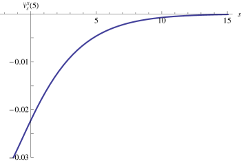
Figure 13: Behavior of $\ddot{v}_{s}(5)$ as a function of $s$ for $s\in(-2,15.08407...)$.

Unfortunately, empirically we know that r.h.s.(75) is not the correct formula for $\ddot{v}_{s}(5)$ when $s\in(15.04807...,\infty)$. Therefore our estimate (79) does not rule out that $\ddot{v}_{s}(5)$ may become positive for some $s\in(15.04807...,\infty)$. We now summarize our computer-generated evidence that $\ddot{v}_{s}(5)<0$ for $s\in(15.04807...,\infty)$.

By our hypotheses, the optimal $5$-point configuration for $s\in(15.04807...,\infty)$ is the square pyramid with adjusted height. So for $s\in(15.04807...,\infty)$ the optimal $5$-point average Riesz $s$-pair-energy is given by ${v}_{s}(5)=\langle V_{s}\rangle(\omega_{\mathrm{sqpyr}}^{s})$, with

$$\hskip-10.0pt\langle V_{s}\rangle(\omega_{\mathrm{sqpyr}}^{s})=\textstyle\frac{1}{s}\left(\frac{2^{1-{s}/{2}}}{5}\big{(}1-z\big{)}^{-\frac{s}{2}}+\frac{2^{1-{s}/{2}}}{5}\big{(}1-z^{2}\big{)}^{-\frac{s}{2}}+\frac{2^{-s}}{5}\big{(}1-z^{2}\big{)}^{-\frac{s}{2}}-1\right),$$ (83)

where $z$ is the unique solution in $(-1,0)$ of the equation

$$\big{(}1+z\big{)}^{1+\frac{s}{2}}+\big{(}2+2^{-{s}/{2}}\big{)}z=0;$$ (84)

the solution of (84) is the “$z$-coordinate” of the base of the pyramid if its tip is at $z=1$. For $s>15$, equation (84) has no explicit solution in terms of elementary functions, but l.h.s.(84) is convex and a Newton scheme very rapidly converges downward from $z_{0}=0$, for all $s>15$. With the help of the Newton scheme we found that

$${v}_{s}(4)-2\langle V_{s}\rangle(\omega_{\mathrm{sqpyr}}^{s})+{v}_{s}(6)<0$$ (85)

for $15<s<10^{6}$. To make this completely rigorous we need to show that asymptotically $\ddot{v}_{s}(5)<0$, with good error bounds, which we hope to supply in future work.

The vindication of Conjecture 3 is complete.

5 An asymptotic point of view

A rigorous proof of the concavity of $N\mapsto v_{s}(N)$ for some regime of $s$-values (possibly for all $s<s_{*}$, with $s_{*}$ conjectured to be in $(-1,0)$) most likely has to be based on a combination of different strategies. Attempts to rigorously identify all the optimizers and to check for the negativity of $\ddot{v}_{s}(N)$ by “explicit computation” may be feasible for sufficiently small $N$-values, but clearly are bound to fail even for moderately large $N$-values. On the other hand, the very-large-$N$ regime is to some extent accessible by asymptotic analysis. Ultimately the goal is to determine the complete asymptotic large-$N$ expansion of $N\mapsto v_{s}(N)$, but at least as many terms as possible. With enough hard work one may be able to extend the asymptotic control down to sufficiently small $N$-values to establish an overlap with some explicitly controlled small-$N$ regime. In the previous section we presented the type of analysis suitable for the small-$N$ regime. This section is devoted to asymptotic analysis.

It has already been mentioned in the introduction that the limit $\displaystyle{\lim_{N\to\infty}}v_{s}(N)$ is given by the variational principle (114). Explicitly

$$\lim_{N\to\infty}v_{s}(N)=\inf_{\mu\in\mathfrak{P}(\mathbb{S}^{2})}{\int\!\!\!\!\int}_{\!\!\!\mathbb{S}^{2}\times\mathbb{S}^{2}}\frac{1}{s}\left(\frac{1}{|{\boldsymbol{{p}}}-{\boldsymbol{{q}}}|^{s}}-1\right)\mu(d{\boldsymbol{{p}}})\mu(d{\boldsymbol{{q}}}),$$ (86)

where $\mathfrak{P}(\mathbb{S}^{2})$ is the set of all Borel probability measures supported on $\mathbb{S}^{2}$. By classical potential theory ([Bjo56] for $s<0$, and [Lan72] for $s>0$) one knows that for $s<2$,

$$\mathcal{I}_{s}[\mu]\equiv\int_{\mathbb{S}^{2}}\int_{\mathbb{S}^{2}}\frac{1}{\left|{\boldsymbol{{p}}}-{\boldsymbol{{q}}}\right|^{s}}\mu(d{\boldsymbol{{p}}})\mu(d{\boldsymbol{{q}}})$$ (87)

is well-defined and finite for any $\mu\in\mathfrak{P}(\mathbb{S}^{2})$. On $\mathfrak{P}(\mathbb{S}^{2})$ the Riesz $s$-energy integral has a degenerate maximum with value $2^{|s|-1}$ when $s\leq-2$, and it has a unique maximum when $-2<s<0$, respectively a unique minimum when $0<s<2$, achieved at the normalized surface area measure $\sigma$ on $\mathbb{S}^{2}\subset\mathbb{R}^{3}$, with value

$$\mathcal{I}_{s}[\sigma]=\frac{2^{1-s}}{2-s}\equiv W_{s};$$ (88)

this expression is also valid at $s=0$, with $\mathcal{I}_{0}[\mu]\equiv 1$ for all $\mu\in\mathfrak{P}(\mathbb{S}^{2})$. For $s\geq 2$ the energy integral (87) is $+\infty$ for any $\mu\in\mathfrak{P}(\mathbb{S}^{2})$. Altogether, therefore,

$$\lim_{N\to\infty}v_{s}(N)=\begin{cases}\frac{1}{s}\left(2^{-s-1}-1\right)&\quad\mbox{if}\quad s\in(-\infty,-2],\\ \frac{1}{s}\left(W_{s}-1\right)&\quad\mbox{if}\quad s\in[-2,2),\\ \infty&\quad\mbox{if}\quad s\in[2,\infty),\end{cases}$$ (89)

with the special case $s=0$ included as $\lim\limits_{s\to 0}\frac{1}{s}\left(W_{s}-1\right)=\frac{1}{2}+\ln\frac{1}{2}$. We need to know how these limiting “values” are approached by $v_{s}(N)$ as $N\to\infty$.

For the regime $s<-2$ we already have an exact formula for $v_{s}(N)$ valid for all even $N$, namely (110). Yet, as mentioned in Appendix A, the $s<-2$ regime is largely unsettled for odd $N$, and we have nothing to add to this here. Moreover, the case $s=-2$ is completely solved, with $v_{-2}(N)$ given by (109). Thus, henceforth we will discuss the regime $s>-2$. Clearly, we need to further make the distinction between the subregimes $s\in(-2,2)$ and $s\geq 2$.

As to the regime $s\in(-2,2)$, to find the large-$N$ asymptotic expansion of $v_{s}(N)$ one seeks the powers $\alpha_{s}\in\mathbb{R}$ and $\beta_{s}\in\mathbb{R}$ for which a nontrivial limit

$$\lim_{N\to\infty}N^{\alpha_{s}}(\ln{N})^{\beta_{s}}\Big{(}v_{s}(N)-\textstyle\frac{1}{s}\left(W_{s}-1\right)\Big{)}=\widehat{C}_{s}$$ (90)

exists; then subtracts $\widehat{C}_{s}$ from the expression under the limit in (90), multiplies by $N^{\alpha_{s}^{\prime}}(\ln{N})^{\beta_{s}^{\prime}}$ with new powers $\alpha_{s}^{\prime}$ and $\beta_{s}^{\prime}$, and repeats the procedure; etc. This strategy has to some extent been carried out in the literature, see [BHS12] for a recent account. We will call upon the results of [BHS12] in a moment. To pave the way for our discussion we first recall the definition (4) of $v_{s}(N)$, involving our standardized Riesz pair-energy $V_{s}(r)$ given in (1), and note that the additive term $\frac{1}{s}$ in the difference $v_{s}(N)-\frac{1}{s}\left(W_{s}-1\right)$ cancels out. This motivates the definition of the $\mathbb{S}^{2}$-adjusted Riesz pair-energy

$$U_{s}(r)\equiv s^{-1}\left(r^{-s}-W_{s}\right),\qquad s<2,\quad s\neq 0,$$ (91)

and its $s\to 0$ limit

$$U_{0}(r)\equiv-\log{r}-W_{\mathrm{log}},$$ (92)

where

$$W_{\mathrm{log}} \equiv\inf\Big{\{}\int_{\mathbb{S}^{2}}\int_{\mathbb{S}^{2}}\log\frac{1}{\left|{\boldsymbol{{p}}}-{\boldsymbol{{q}}}\right|}\mu(d{\boldsymbol{{p}}})\mu(d{\boldsymbol{{q}}}):\mu\in\mathfrak{P}(\mathbb{S}^{2})\Big{\}}$$

is the $s$-derivative of

$$\textstyle W_{s}=1+\left(\frac{1}{2}-\log 2\right)s+\mathcal{O}(s^{2})\qquad{\mathrm{as}}\quad s\to 0,$$

evaluated at $s=0$, with value $W_{\mathrm{log}}(=W_{0}^{\prime})=\frac{1}{2}+\log\frac{1}{2}=-0.193147...<0$.

We define the average $\mathbb{S}^{2}$-adjusted Riesz pair-energy of a configuration by

$$\langle U_{s}\rangle(\omega_{N})\equiv\frac{2}{N\left(N-1\right)}\mathop{\sum\sum}_{1\leq j<k\leq N}U_{s}(\left|{\boldsymbol{{q}}}_{j}-{\boldsymbol{{q}}}_{k}\right|),\quad s\in(-2,2),$$ (93)

and the minimal average $\mathbb{S}^{2}$-adjusted Riesz pair-energy by

$$u_{s}(N)\equiv\inf_{\omega_{N}\subset\mathbb{S}^{2}}\langle U_{s}\rangle(\omega_{N}),\quad s\in(-2,2).$$ (94)

We note that for each $s\in(-2,2)$ the map $N\mapsto u_{s}(N)$ is monotonically increasing and that, by construction, the limit is $0$. Hence $u_{s}(N)\leq 0$ for all $N$.

As for the regime $s\geq 2$, since $v_{s}(N)\to\infty$ as $N\to\infty$, it would seem that the asymptotic analysis has to be set up in a somewhat different manner. In fact, this is true for $s=2$ (see below). However, it is worth noting that r.h.s.(88) is defined on the complex $s$-plane except at the single and simple pole at $s=2$ and thus gives the analytic continuation of $W_{s}$ to the complex $s$-plane. We will denote this meromorphic function by the same symbol, $W_{s}$. Understood in this analytically extended way, (90) and the ensuing description, the definition (91), as well as (93) and (94), all make sense also for the regime $s>2$. Note, though, that for $s>2$ the map $N\mapsto u_{s}(N)$ diverges monotonically to $+\infty$ as $N\to\infty$ (hence $u_{s}(N)\not\leq 0$ for most $N$ when $s>2$), so that the power $\alpha_{s}\leq 0$ for $s>2$ (and if $\alpha_{s}=0$, then $\beta_{s}<0$), while for $s<2$ the power $\alpha_{s}\geq 0$ (and if $\alpha_{s}=0$, then $\beta_{s}>0$). While all this may seem just like a convenient coincidence, we shall see in Subsection 5.2 that the analytic continuation to $s>2$ actually seems to have some deeper significance for the aysmptotic problem; cf. [BHS12].

As to the singular case $s=2$, it obviously makes no sense to subtract the infinite term “$\frac{1}{2}W_{2}$” from $v_{2}(N)$, or from $V_{2}(r)$. Yet, if one replaces (90) by

$$\lim_{N\to\infty}N^{\alpha_{2}}(\ln{N})^{\beta_{2}}\big{(}v_{2}(N)+\textstyle\frac{1}{2}\big{)}=\widehat{C}_{2};$$ (95)

the ensuing description remains valid, with the definitions (93) and (94) extended to $s=2$ with the help of the definition $U_{2}(r)\equiv\frac{1}{2}\frac{1}{r^{2}}$. Note that $N\mapsto u_{2}(N)$ diverges monotonically to $+\infty$ as $N\to\infty$, so the same remarks apply as for the hypersingular regime $s>2$ regarding the powers $\alpha_{s}$ and $\beta_{s}$.

Clearly, for each $s\in(-2,\infty),\,s\neq 2$, the $\mathbb{S}^{2}$-adjusted pair-energy $U_{s}(r)$ on $\mathbb{S}^{2}$ and the standardized pair-energy $V_{s}(r)$ differ only by a constant, viz.

$$U_{s}(r)=V_{s}(r)+s^{-1}({1-W_{s}}),\quad r>0,$$ (96)

with the case $s=0$ understood as limit $s\to 0$, viz. $U_{0}(r)=V_{0}(r)+W_{\rm{log}}$. As a consequence, all their discrete $N$-derivatives coincide; in particular, we have

Lemma 1.

For all $s>-2$ ($s\neq 2$) we have

$$\dot{u}_{s}^{\pm}(N) =\dot{v}_{s}^{\pm}(N),$$ (97)

$$\ddot{u}_{s}(N) =\ddot{v}_{s}(N).$$ (98)

In the remaining subsections we will elaborate on the asymptotic expansion of $N\mapsto u_{s}(N)$ and its implications for the asymptotic expansion of $N\mapsto\ddot{v}_{s}(N)$. Subsection 5.1 is concerned with the potential regime $s\in(-2,2)$, Subsection 5.2 with the hypersingular regime $s>2$, and Subsection 5.3 with the singular case $s=2$. As mentioned earlier, a discussion of the “degeneracy regime” $s\leq-2$ has to be left for some future work.

5.1 The potential-theoretical regime $-2<s<2$

5.1.1 The non-logarithmic cases

In the non-logarithmic cases one has the following bounds for $u_{s}(N)$.

Proposition 10.

Let $-2<s<2$ with $s\neq 0$. Then there exist positive $s$-dependent constants $C>c>0$ such that for all sufficiently large $N\geq 2$

$$\frac{1}{s}\,\frac{W_{s}-c\,N^{s/2}}{N-1} \leq u_{s}(N)\leq\frac{1}{s}\,\frac{W_{s}-C\,N^{s/2}}{N-1} -2<s<0$$ if ,

$$\frac{1}{s}\,\frac{W_{s}-C\,N^{s/2}}{N-1} \leq u_{s}(N)\leq\frac{1}{s}\,\frac{W_{s}-c\,N^{s/2}}{N-1} 0<s<2$$ if .

Proof.

We will call upon the results of [BHS12] and references cited therein. To facilitate the identification of the relevant results in the pertinent literature, we introduce the optimal Riesz $s$-energy of $N$ points on $\mathbb{S}^{2}$, defined for $s\neq 0$ by

$${\mathpzc{E}}_{s}(\mathbb{S}^{2},N)\equiv\mathrm{sign}\,(s)\inf\Big{\{}2\mathop{\sum\sum}_{1\leq j<k\leq N}\frac{\mathrm{sign}\,(s)}{\left|{\boldsymbol{{q}}}_{j}-{\boldsymbol{{q}}}_{k}\right|^{s}}:\{{\boldsymbol{{q}}}_{1},\dots,{\boldsymbol{{q}}}_{N}\}\subset\mathbb{S}^{2}\Big{\}},$$

cf. [HaSa04]. Then it is known (cf. [BHS12]) that there are $s$-dependent constants $C>c>0$ such that

$$-C\,N^{1+s/2}\leq{\mathpzc{E}}_{s}(\mathbb{S}^{2},N)-W_{s}\,N^{2}\leq-c\,N^{1+s/2}$$

for all sufficiently large $N\geq 2$. Hence

$$-C\,\frac{N^{1+s/2}}{N(N-1)}\leq\frac{{\mathpzc{E}}_{s}(\mathbb{S}^{2},N)}{N(N-1)}-W_{s}+\left(1-\frac{N^{2}}{N(N-1)}\right)W_{s}\leq-c\,\frac{N^{1+s/2}}{N(N-1)},$$

or, equivalently,

$$\frac{W_{s}-C\,N^{s/2}}{N-1}\leq\frac{{\mathpzc{E}}_{s}(\mathbb{S}^{2},N)}{N(N-1)}-W_{s}\leq\frac{W_{s}-c\,N^{s/2}}{N-1}.$$

The desired relations follow by multiplying the last relations with $1/s$ and using the definition of the $\mathbb{S}^{2}$-adjusted Riesz pair-energy. ∎

From the bounds in Proposition 10 we get estimates for the discrete second derivative of $u_{s}(N)$ (and by means of Lemma 1 for $v_{s}(N)$).

Proposition 11.

Let $s\in(-2,2),\,s\neq 0$. Let $c$ and $C$ be the constants from Proposition 10. For $s\in(-2,0)$ the discrete second derivative of $u_{s}(N)$ satisfies

$$\ddot{u}_{s}(N)\leq-\frac{2(C-c)}{s}\,\frac{N^{s/2}}{N-1}+\frac{W_{s}}{s}\,\frac{1}{N(N-1)(N-2)}-\frac{C}{s}\frac{N^{s/2}H_{s}(N)}{N(N-1)(N-2)},$$

where $H_{s}(N)\to(2-s)(4-s)>0$ as $N\to\infty$. The right-hand side becomes a lower bound by interchanging $c$ and $C$.

The bounds for $0<s<2$ are obtained by interchanging $c$ and $C$ in the bounds for $\ddot{u}_{s}(N)$ with $-2<s<0$.

Proof.

Let $-2<s<0$. First, we consider the upper bound. By the definition of $\ddot{u}_{s}(N)$ and Proposition 10

$$\ddot{u}_{s}(N) \leq\frac{1}{s}\,\frac{W_{s}-C\,(N-1)^{s/2}}{N-2}-\frac{2}{s}\,\frac{W_{s}-c\,N^{s/2}}{N-1}+\frac{1}{s}\,\frac{W_{s}-C\,(N+1)^{s/2}}{N}$$

$$=\frac{W_{s}}{s}\left[\frac{1}{N-2}-\frac{2}{N-1}+\frac{1}{N}\right]$$

$$\quad-\frac{1}{s}\left\{\frac{C(N-1)^{s/2}}{N-2}-\frac{2cN^{s/2}}{N-1}+\frac{C(N+1)^{s/2}}{N}\right\}$$

$$=-\frac{2(C-c)}{s}\,\frac{N^{s/2}}{N-1}+\frac{W_{s}}{s}\,\frac{1}{N(N-1)(N-2)}$$

$$\quad-\frac{C}{s}\left\{\frac{(N-1)^{s/2}}{N-2}-\frac{2N^{s/2}}{N-1}+\frac{(N+1)^{s/2}}{N}\right\}.$$

Since the function (using the integral representation of the gamma function)

$$f(x)\equiv\frac{x^{s/2}}{x-1}=\sum_{n=0}^{\infty}\frac{1}{x^{n+1-s/2}}=\int_{0}^{\infty}e^{-xt}\sum_{n=0}^{\infty}\frac{t^{n-s/2}}{\Gamma(n+1-s/2)}\,dt,\quad x>1,$$

is strictly monotonically decreasing and convex, the last expression in braces is strictly positive. Series expansion (assisted by mathematica) reveals

$$\frac{(N-1)^{s/2}}{N-2}-\frac{2N^{s/2}}{N-1}+\frac{(N+1)^{s/2}}{N}=\frac{N^{s/2}\left\{(2-s)(4-s)-\frac{s(s-4)}{2}N^{-1}+\cdots\right\}}{N(N-1)(N-2)}.$$

Thus

$$\ddot{u}_{s}(N)\leq-\frac{2(C-c)}{s}\,\frac{N^{s/2}}{N-1}+\frac{W_{s}}{s}\,\frac{1}{N(N-1)(N-2)}-\frac{C}{s}\frac{N^{s/2}H_{s}(N)}{N(N-1)(N-2)},$$

where $H_{s}(N)\to(2-s)(4-s)>0$ as $N\to\infty$.

For a lower bound one has to interchange $C$ and $c$.

For $s\in(0,2)$, the above computations hold with $c$ and $C$ interchanged. ∎

Proposition 11, although much weaker than Proposition 1, clearly shows that one needs more information about the asymptotic behavior of $u_{s}(N)$ for large $N$.

The investigation of the asymptotic behavior of ${\mathpzc{E}}_{s}(\mathbb{S}^{2},N)$ for large $N$ yields the following fundamental conjecture. (We refer the interested reader to [BHS12] and papers cited therein.)

Conjecture 4.

Let $-2<s<2$ and $s\neq 0$. Then there exists a constant $C_{s}$ and a function $\Omega_{s}(N)$ such that

$$u_{s}(N)=\frac{1}{s}\frac{C_{s}}{(4\pi)^{s/2}}\,N^{s/2-1}+\frac{W_{s}}{s}N^{-1}+\Omega_{s}(N)\quad\text{for all $N\geq 2$}$$

and $N^{1-s/2}\Omega_{s}(N)\to 0$ as $N\to\infty$.

It should be noted that the $N^{-1}$-term may be dominated by the function $\Omega_{s}(N)$ for $0<s<2$. Indeed, at presence it is unclear how fast $N^{1-s/2}\Omega_{s}(N)$ tends to zero as $N\to\infty$. One suggestion is that $N^{(s-1)/2-1}$ (or even $N^{s/2-2}$) is the correct order of $N$ for the next term. The numerical evidence is inconclusive in this regard. Worse, the properly normalized $\Omega_{s}(N)$ may be oscillating with bounded non-zero amplitude as $N$ becomes large.

Motivation of Conjecture 4.

For $-2<s<2$ and $s\neq 0$, the following conjecture for the large-$N$ behavior of ${\mathpzc{E}}_{s}(\mathbb{S}^{2},N)$ is known (cf. [BHS12] for a most recent account)

$${\mathpzc{E}}_{s}(\mathbb{S}^{2},N)=W_{s}\,N^{2}+\frac{C_{s}}{(4\pi)^{s/2}}\,N^{1+s/2}+\mathcal{R}_{s}(N),$$

where $\mathcal{R}_{s}(N)\big{/}N^{1+s/2}\to 0$ as $N\to\infty$. Hence,

$$u_{s}(N) =\frac{1}{s}\left\{\frac{{\mathpzc{E}}_{s}(\mathbb{S}^{2},N)}{N(N-1)}-W_{s}\right\}$$

$$=\frac{1}{s}\left\{\left(\frac{N}{N-1}-1\right)W_{s}+\frac{C_{s}}{(4\pi)^{s/2}}\frac{N^{1+s/2}}{N(N-1)}+\frac{\mathcal{R}_{s}(N)}{N(N-1)}\right\}$$

$$=\frac{1}{s}\left\{\frac{C_{s}}{(4\pi)^{s/2}}\,N^{s/2-1}+W_{s}\,N^{-1}+\frac{W_{s}+\frac{C_{s}}{(4\pi)^{s/2}}\,N^{s/2}+\mathcal{R}_{s}(N)}{N(N-1)}\right\}$$

$$=\frac{1}{s}\frac{C_{s}}{(4\pi)^{s/2}}\,N^{s/2-1}+\frac{W_{s}}{s}\,N^{-1}+\Omega_{s}(N),$$

where

$$\Omega_{s}(N)=\frac{1}{N(N-1)}\left\{\frac{W_{s}}{s}+\frac{1}{s}\frac{C_{s}}{(4\pi)^{s/2}}\,N^{s/2}+\frac{1}{s}\frac{\mathcal{R}_{s}(N)}{N^{1+s/2}}\,N^{1+s/2}\right\}.$$

By the assumption on $\mathcal{R}_{s}(N)$ it follows that $N^{1-s/2}\Omega_{s}(N)\to 0$ as $N\to\infty$. ∎

Conjecture 4 imposes the following large-$N$ behavior for the discrete second derivative of $u_{s}(N)$.

Corollary 3.

Let $-2<s<2$ with $s\neq 0$. Under the assumption that Conjecture 4 is true, there holds

$$\ddot{u}_{s}(N)=\frac{(1-s/2)(2-s/2)}{s}\,\frac{C_{s}}{(4\pi)^{s/2}}\,N^{s/2-3}+\frac{2}{s}W_{s}\,N^{-3}+\ddot{\Omega}_{s}(N)+F_{s}(N)$$ (100)

with $N^{4-s/2}F_{s}(N)\to 0$ as $N\to\infty$.

Proof.

By the definition of the discrete second derivative (cf. (6))

$$\ddot{u}_{s}(N) =\frac{1}{s}\,\frac{C_{s}}{(4\pi)^{s/2}}\,N^{s/2-1}\left\{\left(1-\frac{1}{N}\right)^{s/2-1}-2-\left(1+\frac{1}{N}\right)^{s/2-1}\right\}$$

$$\phantom{=}+\frac{W_{s}}{s}\,N^{-1}\left\{\left(1-\frac{1}{N}\right)^{-1}-2-\left(1+\frac{1}{N}\right)^{-1}\right\}+\ddot{\Omega}_{s}(N).$$

Series expansion gives (here ${\left(a\right)_{n}}$ is the Pochhammer symbol or rising factorial)

$$\Big{(}1-\frac{1}{N}\Big{)}^{s/2-1}-2-\Big{(}1+\frac{1}{N}\Big{)}^{s/2-1}=\sum_{n=1}^{\infty}\frac{{\left(1-s/2\right)_{n}}}{n!}\,\frac{1+(-1)^{n}}{N^{n}}$$

and simplification yields

$$\Big{(}1-\frac{1}{N}\Big{)}^{-1}-2-\Big{(}1+\frac{1}{N}\Big{)}^{-1}=\frac{2}{N^{2}-1}.$$

Hence

$$\ddot{u}_{s}(N)=\frac{{\left(1-s/2\right)_{2}}}{s}\,\frac{C_{s}}{(4\pi)^{s/2}}\,N^{s/2-3}+\frac{2}{s}W_{s}\,N^{-3}+\ddot{\Omega}_{s}(N)+F_{s}(N),$$

where

$$\begin{split}F_{s}(N)&\equiv\frac{1}{s}\,\frac{C_{s}}{(4\pi)^{s/2}}\,N^{s/2-1}\Big{[}\Big{(}1-\frac{1}{N}\Big{)}^{s/2-1}\!\!-2-\Big{(}1+\frac{1}{N}\Big{)}^{s/2-1}\!\!-\frac{{\left(1-s/2\right)_{2}}}{N^{2}}\Big{]}\\ &\phantom{=}+\frac{W_{s}}{s}\,\frac{2}{N^{3}(N^{2}-1)}\end{split}$$

and $N^{4-s/2}F_{s}(N)\to 0$ as $N\to\infty$, since $-2<s<2$. ∎

Remark 15.

For $-2<s<0$ the dominant term in (100) is $(2W_{s}/s)N^{-3}$ or possibly $\ddot{\Omega}_{s}(N)$. Thus, for sufficiently large $N$ the sign of $\ddot{u}_{s}(N)$ is negative or interference from higher order terms in the conjectured asymptotic expansion of $u_{s}(N)$ forces a positive sign. The numerical evidence for $s=-1$ (no exceptional $N<200$ with non-negative discrete second derivative of $v_{-1}(N)$) discussed earlier supports a negative sign of $\ddot{v}_{-1}(N)$, viz. $\ddot{u}_{-1}(N)$. In fact, if $\ddot{u}_{s}(N)\geq 0$ for infinitely many growing $N_{k}$, then (100) would imply that

$$\ddot{\Omega}_{s}(N_{k})=\Omega_{s}(N_{k}-1)-2\Omega_{s}(N_{k})+\Omega_{s}(N_{k}+1)\geq-\textstyle\frac{2}{s}W_{s}N_{k}^{-3}>0.$$

Remark 16.

For $0<s<2$ the dominant term in (100) is the $C_{s}$-term or possibly $\ddot{\Omega}_{s}(N)$. It is not even known that the constant $C_{s}$ appearing in Conjecture 4 and thus in (100) exists. Results for the hypersingular case discussed below suggest that $C_{s}$ is related to the Epstein zeta function for the hexagonal lattice in the plane. An inspection of the graph of the conjectured value of $C_{s}$, analytically continued, shows that it is negative in the interval $(0,2)$! Asymptotically seen, higher-order terms in the large-$N$ expansion of $u_{s}(N)$, $0<s<2$ cause the appearance of “large” magic numbers $N$. Indeed, analysis of the putatively minimal average $\mathbb{S}^{2}$-adjusted Riesz pair-energy up to $N=200$ for $s=1$ gives a sequence of $N$’s for which $\ddot{u}_{s}(N)$ is not negative.

5.1.2 The logarithmic case

In the logarithmic case one has the following bounds for $u_{0}(N)$.

Proposition 12.

There exist positive constants $C>c>0$ such that for all sufficiently large $N$

$$\frac{W_{\mathrm{log}}-\frac{1}{2}\log N-C\,N}{N(N-1)}\leq u_{0}(N)\leq\frac{W_{\mathrm{log}}-\frac{1}{2}\log N-c\,N}{N(N-1)}.$$

Proof.

Let ${\mathpzc{E}}_{\mathrm{log}}(\mathbb{S}^{2},N)$ be defined by

$${\mathpzc{E}}_{\mathrm{log}}(\mathbb{S}^{2},N)\equiv\inf\Big{\{}2\textstyle\mathop{\sum\sum}\limits_{1\leq j<k\leq N}\log\frac{1}{\left|{\boldsymbol{{q}}}_{j}-{\boldsymbol{{q}}}_{k}\right|}:\{{\boldsymbol{{q}}}_{1},\dots,{\boldsymbol{{q}}}_{N}\}\subset\mathbb{S}^{2}\Big{\}}.$$

Then it is known that there are constants $C>c>0$ such that (cf. [BHS12])

$$-C\,N\leq{\mathpzc{E}}_{\mathrm{log}}(\mathbb{S}^{2},N)-W_{\mathrm{log}}\,N^{2}+\textstyle\frac{1}{2}N\log N\leq-c\,N$$

for all sufficiently large $N\geq 2$. Hence

$$\frac{-\frac{1}{2}\log N-C\,N}{N(N-1)}\leq\frac{{\mathpzc{E}}_{\mathrm{log}}(\mathbb{S}^{2},N)}{N(N-1)}-W_{\mathrm{log}}-\frac{1}{N-1}W_{\mathrm{log}}\leq\frac{-\frac{1}{2}\log N-c\,N}{N(N-1)}.$$

The desired bounds follow. ∎

Proposition 12 provides the following weak bounds for the discrete second derivative of $u_{0}(N)$ (and by means of Lemma 1 for $v_{s}(N)$).

Proposition 13.

Let $c$ and $C$ be the constants from Proposition 12. Then

$$\begin{split}\ddot{u}_{0}(N)&\leq\frac{2(C-c)}{N-1}-\frac{2c}{N(N-1)(N-2)}\\ &\phantom{=}-\frac{3\log N}{(N+1)N(N-1)(N-2)}+\frac{6W_{\mathrm{log}}+H_{0}(N)}{(N+1)N(N-1)(N-2)},\end{split}$$

where $H_{0}(N)\to 5/2$ as $N\to\infty$.

For the corresponding lower bound one has to interchange $c$ and $C$.

Proof.

First we consider the upper bound. By the definition of $\ddot{u}_{0}(N)$ and Proposition 12

$$\ddot{u}_{0}(N) \leq\frac{W_{\mathrm{log}}-\frac{1}{2}\log(N-1)-c\,(N-1)}{(N-1)(N-2)}-2\frac{W_{\mathrm{log}}-\frac{1}{2}\log N-C\,N}{N(N-1)}$$

$$\phantom{=}+\frac{W_{\mathrm{log}}-\frac{1}{2}\log(N+1)-c\,(N+1)}{(N+1)N}$$

$$=W_{\mathrm{log}}\left(\frac{1}{(N-1)(N-2)}-2\frac{1}{N(N-1)}+\frac{1}{(N+1)N}\right)$$

$$\phantom{=}-\frac{1}{2}\left[\frac{\log(N-1)}{(N-1)(N-2)}-2\frac{\log N}{N(N-1)}+\frac{\log(N+1)}{(N+1)N}\right]$$

$$\phantom{=}-\left\{\frac{c}{N-2}-2\frac{C}{N-1}+\frac{c}{N}\right\}.$$

Simplification (assisted by mathematica) gives for the expression in parenthesis

$$\frac{6}{(N+1)N(N-1)(N-2)},$$

for the expression in braces

$$-2\frac{C-c}{N-1}+c\left(\frac{1}{N-2}-\frac{2}{N-1}+\frac{1}{N}\right)=-2\frac{C-c}{N-1}+\frac{2c}{N(N-1)(N-2)}$$

and for the square-bracketed expression (using series expansion)

$$\begin{split}&\frac{6\log N}{(N+1)N(N-1)(N-2)}+\frac{\log(1-\frac{1}{N})}{(N-1)(N-2)}+\frac{\log(1+\frac{1}{N})}{(N+1)N}\\ &\phantom{equals}=\frac{6\log N}{(N+1)N(N-1)(N-2)}+\frac{-\frac{5}{N^{2}}+\frac{8}{N^{3}}+\cdots}{(N-1)(N-2)}.\end{split}$$

Putting everything together, we arrive at

$$\begin{split}\ddot{u}_{0}(N)&\leq\frac{2(C-c)}{N-1}-\frac{2c}{N(N-1)(N-2)}\\ &\phantom{=}-\frac{3\log N}{(N+1)N(N-1)(N-2)}+\frac{6W_{\mathrm{log}}+\frac{5}{2}-\frac{3}{2N}+\dots}{(N+1)N(N-1)(N-2)}.\end{split}$$

For the corresponding lower bound one has to interchange $c$ and $C$. ∎

The investigation of the asymptotic behavior of ${\mathpzc{E}}_{\mathrm{log}}(\mathbb{S}^{2},N)$ provides the following conjecture.

Conjecture 5.

There exists a constant $C_{\mathrm{log}}$ and a function $\Omega_{0}(N)$ such that

$$u_{0}(N)=-\frac{1}{2}\frac{\log N}{N}+\frac{W_{\mathrm{log}}+C_{\mathrm{log}}}{N}-\frac{1}{2}\frac{\log N}{N^{2}}+\frac{W_{\mathrm{log}}+C_{\mathrm{log}}}{N^{2}}+\Omega_{0}(N)\quad\forall N\geq 2,$$

where $N\Omega_{0}(N)\to 0$ (or in its stronger form $N^{2}\Omega_{0}(N)\to c_{0}\neq 0$) as $N\to\infty$.

The constant $C_{\mathrm{log}}$ is given by

$$C_{\mathrm{log}}=2\log 2+\frac{1}{2}\log\frac{2}{3}+3\log\frac{\sqrt{\pi}}{\Gamma(1/3)}=-0.05560530494339251850\ldots<0.$$

Motivation of Conjecture 5.

The following conjecture for the large-$N$ behavior of ${\mathpzc{E}}_{\mathrm{log}}(\mathbb{S}^{2},N)$ is known (cf. [BHS12] for a most recent account)

$${\mathpzc{E}}_{\mathrm{log}}(\mathbb{S}^{2},N)=W_{\mathrm{log}}\,N^{2}-\frac{1}{2}N\log N+C_{\mathrm{log}}\,N+\mathcal{R}_{\mathrm{log}}(N),$$

where $\mathcal{R}_{\mathrm{log}}(N)\big{/}N\to 0$ as $N\to\infty$. A stronger form states that $\mathcal{R}_{\mathrm{log}}(N)$ converges to a non-zero constant. Hence

$$u_{0}(N) =\frac{{\mathpzc{E}}_{\mathrm{log}}(\mathbb{S}^{2},N)}{N(N-1)}-W_{\mathrm{log}}$$

$$=\underbrace{\left(\frac{N^{2}}{N(N-1)}-1\right)}_{1/(N-1)}W_{\mathrm{log}}-\frac{1}{2}\frac{\log N}{N-1}+\frac{C_{\mathrm{log}}}{N-1}+\frac{\mathcal{R}_{\mathrm{log}}(N)}{N(N-1)}$$

$$=-\frac{1}{2}\frac{\log N}{N}+\frac{W_{\mathrm{log}}+C_{\mathrm{log}}}{N}-\frac{1}{2}\frac{\log N}{N^{2}}+\frac{W_{\mathrm{log}}+C_{\mathrm{log}}}{N^{2}}+\Omega_{0}(N),$$

where we used that

$$\frac{1}{N-1}=\frac{1}{N}+\frac{1}{N(N-1)}=\frac{1}{N}+\frac{1}{N^{2}}+\frac{1}{N^{2}(N-1)}$$

and

$$\Omega_{0}(N)\equiv\frac{1}{N(N-1)}\left\{\mathcal{R}_{\mathrm{log}}(N)-\frac{1}{2}\frac{\log N}{N}+\frac{W_{\mathrm{log}}}{N}\right\}.$$

From the assumptions on $\mathcal{R}_{\mathrm{log}}(N)$ it follows that $N\Omega_{0}(N)\to 0$ (or in its stronger form $N^{2}\Omega_{0}(N)\to c_{0}\neq 0$) as $N\to\infty$. ∎

Conjecture 5 implies the following large-$N$ behavior for the discrete second derivative of $u_{0}(N)$.

Corollary 4.

Under the assumption that Conjecture 5 is true, there holds

$$\ddot{u}_{0}(N)=-\frac{\log N}{N^{3}}+\frac{3/2+W_{\mathrm{log}}+C_{\mathrm{log}}}{N^{3}}+\ddot{\Omega}_{0}(N)+F_{0}(N),$$ (101)

with $N^{4-\epsilon}F_{0}(N)\to 0$ as $N\to\infty$ for any $\epsilon>0$.

Note that $3/2+W_{\mathrm{log}}+C_{\mathrm{log}}>0$.

Proof.

By the definition of the discrete second derivative (cf. (6))

$$\ddot{u}_{0}(N) =-\frac{1}{2}\left(\frac{\log(N-1)}{N-1}-2\frac{\log N}{N}+\frac{\log(N+1)}{N+1}\right)$$

$$\phantom{=}+\left(W_{\mathrm{log}}+C_{\mathrm{log}}\right)\left[\frac{1}{N-1}-2\frac{1}{N}+\frac{1}{N+1}\right]$$

$$\phantom{=}-\frac{1}{2}\left(\frac{\log(N-1)}{(N-1)^{2}}-2\frac{\log N}{N^{2}}+\frac{\log(N+1)}{(N+1)^{2}}\right)$$

$$\phantom{=}+\left(W_{\mathrm{log}}+C_{\mathrm{log}}\right)\left[\frac{1}{(N-1)^{2}}-2\frac{1}{N^{2}}+\frac{1}{(N+1)^{2}}\right]+\ddot{\Omega}_{0}(N).$$

The series expansions

$$\Big{(}1-\frac{1}{N}\Big{)}^{-\alpha}=\sum_{n=0}^{\infty}\frac{{\left(\alpha\right)_{n}}}{n!}\frac{1}{N^{n}}$$

and

$$\log\Big{(}1-\frac{1}{N}\Big{)}\Big{(}1-\frac{1}{N}\Big{)}^{-\alpha} =-\sum_{k=1}^{\infty}\sum_{n=0}^{\infty}\frac{1}{k}\frac{{\left(\alpha\right)_{n}}}{n!}\frac{1}{N^{k+n}}$$

$$=-\sum_{\ell=1}^{\infty}\left\{\sum_{n=0}^{\ell-1}\frac{1}{\ell-n}\frac{{\left(\alpha\right)_{n}}}{n!}\right\}\frac{1}{N^{\ell}}$$

yield

$$\frac{1}{N-1}-\frac{2}{N}+\frac{1}{N+1} =\frac{1}{N}\left(\frac{1}{1-\frac{1}{N}}-2+\frac{1}{1+\frac{1}{N}}\right)=\frac{1}{N}\sum_{n=2}^{\infty}\frac{1+(-1)^{n}}{N^{n}}$$

and thus

$$\frac{\log(N-1)}{N-1}-2\frac{\log N}{N}+\frac{\log(N+1)}{N+1}$$

$$\phantom{XX}=\log N\!\left[\!\frac{1}{N-1}-2\frac{1}{N}+\frac{1}{N+1}\!\right]+\frac{1}{N}\left[\!\frac{\log(1-\frac{1}{N})}{1-\frac{1}{N}}+\frac{\log(1+\frac{1}{N})}{1+\frac{1}{N}}\!\right]$$

$$\phantom{XX}=\frac{\log N}{N^{3}}\sum_{n=0}^{\infty}\frac{1+(-1)^{n}}{N^{n}}-\sum_{\ell=2}^{\infty}H_{\ell}\frac{1+(-1)^{\ell}}{N^{\ell+1}},$$

where $H_{\ell}$ denotes the $\ell$-th Harmonic number $H_{\ell}\equiv\sum_{k=1}^{\ell}\frac{1}{k}$; furthermore

$$\frac{1}{(N-1)^{2}}-2\frac{1}{N^{2}}+\frac{1}{(N+1)^{2}}=\frac{1}{N^{2}}\left(\frac{1}{(1-\frac{1}{N})^{2}}-2+\frac{1}{(1+\frac{1}{N})^{2}}\right)$$

$$\phantom{equals}=\frac{1}{N^{2}}\sum_{n=2}^{\infty}\frac{{\left(2\right)_{n}}}{n!}\frac{1+(-1)^{n}}{N^{n}}=\sum_{n=2}^{\infty}(n+1)\frac{1+(-1)^{n}}{N^{n+2}}$$

and thus

$$\frac{\log(N-1)}{(N-1)^{2}}-2\frac{\log N}{N^{2}}+\frac{\log(N+1)}{(N+1)^{2}}$$

$$\phantom{eq}=\log N\left(\frac{1}{(N-1)^{2}}-2\frac{1}{N^{2}}+\frac{1}{(N+1)^{2}}\right)$$

$$\phantom{equa}+\frac{1}{N^{2}}\left(\frac{\log(1-\frac{1}{N})}{(1-\frac{1}{N})^{2}}+\frac{\log(1+\frac{1}{N})}{(1+\frac{1}{N})^{2}}\right)$$

$$\phantom{eq}=\frac{\log N}{N^{4}}\sum_{n=0}^{\infty}(n+3)\frac{1+(-1)^{n}}{N^{n}}-\sum_{\ell=2}^{\infty}\left\{\sum_{n=0}^{\ell-1}\frac{1}{\ell-n}\frac{{\left(2\right)_{n}}}{n!}\right\}\frac{1+(-1)^{\ell}}{N^{\ell+2}}.$$

Combining everything (and shifting indices of summations), we arrive at

$$\ddot{u}_{0}(N) =-\frac{1}{2}\left(\frac{\log N}{N^{3}}\sum_{n=0}^{\infty}\frac{1+(-1)^{n}}{N^{n}}-\frac{1}{N^{3}}\sum_{\ell=0}^{\infty}H_{\ell+2}\frac{1+(-1)^{\ell}}{N^{\ell}}\right)$$

$$\phantom{=}+\frac{W_{\mathrm{log}}+C_{\mathrm{log}}}{N^{3}}\sum_{n=0}^{\infty}\frac{1+(-1)^{n}}{N^{n}}$$

$$\phantom{=}-\frac{\log N}{2N^{4}}\sum_{n=0}^{\infty}(n+3)\frac{1+(-1)^{n}}{N^{n}}$$

$$\phantom{=}+\frac{1}{2N^{4}}\sum_{\ell=0}^{\infty}\left\{\sum_{n=0}^{\ell+1}\frac{n+1}{\ell+2-n}\right\}\frac{1+(-1)^{\ell}}{N^{\ell}}$$

$$\phantom{=}+\frac{W_{\mathrm{log}}+C_{\mathrm{log}}}{N^{4}}\sum_{n=0}^{\infty}(n+3)\frac{1+(-1)^{n}}{N^{n}}$$

$$\phantom{=}+\ddot{\Omega}_{0}(N).$$

Rearranging the terms gives

$$\ddot{u}_{0}(N)=-\frac{\log N}{N^{3}}+\frac{3/2+W_{\mathrm{log}}+C_{\mathrm{log}}}{N^{3}}+\ddot{\Omega}_{0}(N)+F_{0}(N),$$

where

$$F_{0}(N) \equiv-\frac{1}{2}\frac{\log N}{N^{3}}\sum_{n=2}^{\infty}\frac{1+(-1)^{n}}{N^{n}}+\frac{1}{2}\frac{1}{N^{3}}\sum_{\ell=2}^{\infty}H_{\ell+2}\frac{1+(-1)^{\ell}}{N^{\ell}}$$

$$\phantom{=}+\frac{W_{\mathrm{log}}+C_{\mathrm{log}}}{N^{3}}\sum_{n=2}^{\infty}\frac{1+(-1)^{n}}{N^{n}}$$

$$\phantom{=}-\frac{\log N}{2N^{4}}\sum_{n=0}^{\infty}(n+3)\frac{1+(-1)^{n}}{N^{n}}$$

$$\phantom{=}+\frac{1}{2N^{4}}\sum_{\ell=0}^{\infty}\left\{\sum_{n=0}^{\ell+1}\frac{n+1}{\ell+2-n}\right\}\frac{1+(-1)^{\ell}}{N^{\ell}}$$

$$\phantom{=}+\frac{W_{\mathrm{log}}+C_{\mathrm{log}}}{N^{4}}\sum_{n=0}^{\infty}(n+3)\frac{1+(-1)^{n}}{N^{n}}$$

with $N^{4-\epsilon}F_{0}(N)\to 0$ as $N\to\infty$ for any $\epsilon>0$. ∎

Remark 17.

The dominant term in (101) is the negative $-(\log N)/N^{3}$ term or possibly $\ddot{\Omega}_{0}(N)$. An increasing infinite sequence of magic numbers $(N_{k})$ with $\ddot{u}_{0}(N_{k})\geq 0$ would be caused by higher-order terms in the conjectured asymptotic expansion of $u_{0}(N)$ and thus would, for example, exclude the hypothetical expansion $\Omega_{0}(N)=c_{0}+\widetilde{\Omega}_{0}(N)$ with $\widetilde{\Omega}_{0}(N)/\big{[}(\log N)/N\big{]}\to 0$ as $N\to\infty$.

5.2 The hypersingular regime $s>2$

For $s>2$ it is proved in Hardin and Saff [HaSa05] that

$$\lim_{N\to\infty}\frac{{\mathpzc{E}}_{s}(\mathbb{S}^{2},N)}{N^{1+s/2}}=\frac{C_{s}}{(4\pi)^{s/2}}$$

for some constant $C_{s}$ depending on $s$. In [KuSa98] it is shown that, for $s>2$,

$$\limsup_{N\to\infty}\frac{{\mathpzc{E}}_{s}(\mathbb{S}^{2},N)}{N^{1+s/2}}\leq\frac{\left(\sqrt{3}/2\right)^{s/2}\operatorname{\zeta}_{\Lambda}(s)}{\left(4\pi\right)^{s/2}},$$

and it is conjectured in [KuSa98] that for $s>2$,

$$C_{s}=\left(\sqrt{3}/2\right)^{s/2}\operatorname{\zeta}_{\Lambda}(s),$$ (102)

where $\operatorname{\zeta}_{\Lambda}$ is the zeta function associated with the hexagonal lattice. The zeta function associated with the hexagonal lattice admits the factorization

$$\textstyle\operatorname{\zeta}_{\Lambda}(s)=6\operatorname{\zeta}\big{(}\frac{s}{2}\big{)}\operatorname{L}_{-3}\big{(}\frac{s}{2}),\qquad\mathop{\mathrm{Re}}s>2,$$

where $\zeta(s)$ is the Riemann zeta function and $\operatorname{L}_{-3}(s)$ a Dirichlet $\operatorname{L}$-Series, viz.

$$\operatorname{\zeta}(s) =1+\frac{1}{2^{s}}+\frac{1}{3^{s}}+\frac{1}{4^{s}}+\frac{1}{5^{s}}+\frac{1}{6^{s}}+\cdots,\qquad\mathop{\mathrm{Re}}s>1,$$

$$\operatorname{L}_{-3}(s) =1-\frac{1}{2^{s}}+\frac{1}{4^{s}}-\frac{1}{5^{s}}+\frac{1}{7^{s}}-\frac{1}{8^{s}}+\cdots,\qquad\mathop{\mathrm{Re}}s>1.$$

For computational purposes it is more convenient to express this Dirichlet $\operatorname{L}$-series in terms of the Hurwitz zeta function

$$\zeta(s,a)\equiv\sum_{k=0}^{\infty}\frac{1}{\left(k+a\right)^{s}},\quad\mathop{\mathrm{Re}}s>1,$$

by means of

$$\operatorname{L}_{-3}(s)=3^{-s}\textstyle{\left[\zeta\big{(}s,\frac{1}{3}\big{)}-\zeta\big{(}s,\frac{2}{3}\big{)}\right].}$$

Using these representations we computed the graph of r.h.s.(102), see Fig. 14.

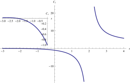
Figure 14: The graph of the right-hand side of (102).

The fundamental conjecture for the asymptotic expansion of ${\mathpzc{E}}_{s}(\mathbb{S}^{2},N)$, $s\in(2,4)$, as $N$ becomes large states that

Conjecture 6.

For $s\in(2,4)$ the asymptotic expansion of ${\mathpzc{E}}_{s}(\mathbb{S}^{2},N)$ reads

$${\mathpzc{E}}_{s}(\mathbb{S}^{2},N)\sim{\big{(}\sqrt{3}/8\pi\big{)}^{s/2}\operatorname{\zeta}_{\Lambda}(s)}\,N^{1+s/2}+W_{s}\,N^{2}+o(N^{2})\quad\text{as $N\to\infty$.}$$

Note the appearance of (the analytically continued) $W_{s}$ as coefficient of the $\mathcal{O}(N^{2})$-term, which now is the next-to-leading-order term.

The fundamental conjecture motivates the introduction of the following $\mathbb{S}^{2}$-re-adjusted pair-energy

$$\widetilde{U}_{s}(r)\equiv s^{-1}\left(r^{-s}-W_{s}-\big{(}\sqrt{3}/8\pi\big{)}^{s/2}\operatorname{\zeta}_{\Lambda}(s)\,N^{s/2-1}\right),\quad s\in(2,4),$$ (103)

the associated average $\mathbb{S}^{2}$-re-adjusted pair-energy of a configuration $\omega_{N}$,

$$\langle\widetilde{U}_{s}\rangle(\omega_{N})\equiv\frac{2}{N\left(N-1\right)}\mathop{\sum\sum}_{1\leq j<k\leq N}\widetilde{U}_{s}(\left|{\boldsymbol{{q}}}_{j}-{\boldsymbol{{q}}}_{k}\right|),\quad s\in(2,4),$$ (104)

and the minimal average $\mathbb{S}^{2}$-re-adjusted Riesz pair-energy, given by

$$\tilde{u}_{s}(N)\equiv\inf_{\omega_{N}\subset\mathbb{S}^{2}}\langle\widetilde{U}_{s}\rangle(\omega_{N}),\quad s\in(2,4).$$ (105)

According to the fundamental conjecture, $\tilde{u}_{s}(N)$ would be bounded above and tend to $0$ when $N\to\infty$, for all $2<s<4$.

However, since $N\mapsto N^{s/2-1}$ is a concave, increasing function for $s\in(2,4)$, it is neither clear whether $N\mapsto\tilde{u}_{s}(N)={u}_{s}(N)-\big{(}\sqrt{3}/8\pi\big{)}{}^{\!\!s/2}\operatorname{\zeta}_{\Lambda}(s)N^{s/2-1}$ is increasing (whereas $N\mapsto{u}_{s}(N)$ is), nor whether $N\mapsto\tilde{u}_{s}(N)$ is concave whenever $N\!\mapsto\!{u}_{s}(N)$ is. These are interesting open problems for future study.

5.3 The singular case $s=2$

Kuijlaars and Saff [KuSa98] showed that

$$\lim_{N\to\infty}\frac{{E}_{2}(N)}{N^{2}\log N}=\frac{1}{4}.$$

A conjecture of Brauchart, Hardin and Saff [BHS12] is that

$$\textstyle{E}_{2}(N)\sim\frac{1}{4}\,N^{2}\log N+C_{2}N^{2}+o(N^{2})\quad\text{as $N\to\infty$,}$$

where

$$\hskip-5.0pt\textstyle C_{2}=\frac{1}{4}\left[\gamma-\log(2\sqrt{3}\pi)\right]+\frac{\sqrt{3}}{4\pi}\left[\gamma_{1}\big{(}\frac{2}{3}\big{)}-\gamma_{1}\big{(}\frac{1}{3}\big{)}\right]=-0.08576841030090...<0.$$

This motivates the introduction of the following $\mathbb{S}^{2}$-re-adjusted pair-energy,

$$\widetilde{U}_{2}(r)\equiv\textstyle\frac{1}{2}\left(r^{-2}-C_{2}-\frac{1}{4}\log N\right),$$ (106)

its associated average $\mathbb{S}^{2}$-re-adjusted pair-energy of a configuration $\omega_{N}$,

$$\langle\widetilde{U}_{2}\rangle(\omega_{N})\equiv\frac{2}{N\left(N-1\right)}\mathop{\sum\sum}_{1\leq j<k\leq N}\widetilde{U}_{2}(\left|{\boldsymbol{{q}}}_{j}-{\boldsymbol{{q}}}_{k}\right|),$$ (107)

and the minimal average $\mathbb{S}^{2}$-re-adjusted Riesz pair-energy at $s=2$, given by

$$\tilde{u}_{2}(N)\equiv\inf_{\omega_{N}\subset\mathbb{S}^{2}}\langle\widetilde{U}_{2}\rangle(\omega_{N}).$$ (108)

By the above conjecture, $\tilde{u}_{2}(N)$ would be bounded and tend to $0$ when $N\to\infty$.

However, since $N\mapsto\log N$ is a concave, increasing function, it is neither clear whether $N\mapsto\tilde{u}_{2}(N)={u}_{2}(N)-C_{2}-\frac{1}{4}\log N$ is increasing (whereas $N\mapsto{u}_{2}(N)$ is) nor whether $N\mapsto\tilde{u}_{2}(N)$ is concave whenever $N\!\mapsto\!{u}_{2}(N)$ is. Also these are interesting open problems for future study.

6 Summary and Outlook

In this paper we have inquired into the local concavity properties of the map $N\mapsto v_{s}(N)$, where $v_{s}(N)$ is the minimal average standardized Riesz pair-energy for $N$-point configurations on the unit 2-sphere $\mathbb{S}^{2}\subset\mathbb{R}^{3}$. By “standardized” Riesz pair-energy we mean $V_{s}(r)=s^{-1}\left(r^{-s}-1\right)$, with $s\in\mathbb{R}$, where $r$ is the chordal distance between the points of the pair. The map $s\mapsto V_{s}(r)$ defines a real analytical family of increasing pair-energies; in particular, it includes the logarithmic interaction $-\ln r=\lim_{s\to 0}V_{s}(r)$.

Given the limited amount of knowledge about true minimizers (see Appendix A), we have studied mostly the $N$-dependence of putatively minimal average standardized Riesz pair-energies $v^{x}_{s}(N)$, obtained numerically in computer experiments. Our empirical findings indicate that for $s=-1$ the minimal average standardized Riesz pair-energy could be locally strictly concave function of $N$, without any “convex anomalies.” However, when $s\in\{0,1,2,3\}$ we have found that $N\mapsto v^{x}_{s}(N)$ is not strictly concave. Based on our empirical findings we have conjectured that there exists an $s_{*}\in(-1,0)$ such that $N\mapsto v^{x}_{s}(N)$ is locally strictly concave for all $s<s_{*}$, while local strict concavity is violated at some $N$-values whenever $s\geq s_{*}$. We presented some rigorous (but rough), and some quasi-rigorous (yet more promising) upper bounds on $s_{*}$. Also, in Appendix A, we shall readily see analytically that $N\mapsto v_{-2}(N)$ is strictly locally concave, and restricted to even numbers $N=2n$, the results of [Bjo56] imply the strict local concavity of $N\mapsto v_{s}(N)$ also for $s<-2$.

We also presented various rigorous bounds on the second discrete derivative, $\ddot{v}_{s}(N)$, of $N\mapsto v_{s}(N)$, and we related concavity to an asymptotic analysis of the large-$N$ regime. Our control of $\ddot{v}_{s}(N)$ is not good enough to prove strict local concavity for any $s$ other than $s=-2$, yet we expect that our analysis will serve as a stepping stone along the way to a concavity proof for $s<s_{*}$. In any event, our rigorous bounds can serve as test criteria for optimality.

We emphasize that an a-priori knowledge of any concavity properties of the actual maps $N\mapsto v_{s}(N)$ will furnish valuable test criteria for the accuracy of empirical maps $N\mapsto v^{x}_{s}(N)$. In particular, given the practical importance of the $s=-1$ problem in numerical integration schemes as mentioned in Appendix A, it is of special interest to prove, or disprove, the empirically suggested local strict concavity of $N\mapsto v_{-1}(N)$. Since the optimizers of the $s=-1$ Fekete problem are related to spherical digital nets, it is of interest to raise our concavity questions also for these average standardized Riesz pair-energies computed for such nets; see our Appendix D.

For each studied $s$-value, the $N$-values at which the map $N\mapsto v^{x}_{s}(N)$ is strictly convex were collected into a set ${\cal C}_{+}^{x}(s)$. Inspection of the empirical map $s\mapsto{\cal C}_{+}^{x}(s)$ suggested to us the conjecture that the actual map $s\mapsto{\cal C}_{+}(s)$ is set-theoretically monotonic increasing. Inspired by this conjecture we suspected, and then verified (by finding lower-energy configuations), that the $N=177$ and $N=197$ data points in the computer-experimental tables of putatively minimal Riesz pair-energies for $s\in\{2,3\}$ in [Cal09] are non-optimal. This makes it plain that a-priori knowledge of any monotonicity property of the map $s\mapsto{\cal C}_{+}(s)$ will also furnish valuable test criteria for the accuracy of empirical maps $N\mapsto v^{x}_{s}(N)$.

We have also discovered yet another empirical monotonicity: the percentage of odd numbers in ${\cal C}_{+}^{x}(s)$ increases monotonically with $s\in\{0,1,2,3\}$. Based on this finding it is reasonable to conjecture that the percentage of odd numbers in ${\cal C}_{+}(s)$ increases monotonically with $s>s_{*}$, if such $s_{*}$ exists.

We have not been able to detect any algebraic generating rule of ${\cal C}_{+}^{x}(s)$ for any $s\in\{0,1,2,3\}$, and with increasing $s$ it seems increasingly unlikely (another monotonicity property!) to detect any such rule, because the sets ${\cal C}_{+}^{x}(s)$ appear more and more random as $s$ increases from $0$ to $3$. On the other hand, the set ${\cal C}_{+}^{x}(0)$ exhibits some intriguing quasi-regular patterns which reminded us of the periodic table of the chemists, or the “magic” numbers in nuclear physics; incidentally, note that the $s=0$ problem can be viewed as the electric ground state energy problem for a system of $N$ “two-dimensional” point charges on $\mathbb{S}^{2}$. Thus we decided to call the $N$-values in ${\cal C}_{+}^{x}(0)$ the “Magic Numbers of Smale’s $7$th Problem.” We have speculated that those “magic” numbers are perhaps associated with “optimally symmetric” endpoints of families of more-and-more symmetric configurations, based on our observation that the first few configurations associated with ${\cal C}_{+}^{x}(0)$ are highly symmetric. In order to switch from a “magic-$N$” optimal configuration to an optimal $N+1$ configuration by adding a particle would then require an unusually large amount of energy to break up the “optimally symmetric (magic-$N$)” configuration — hence the convexity.

We hope that our paper triggers further research into the concavity properties of the minimial average standardized Riesz pair-energies on $\mathbb{S}^{2}$, in particular the structure of its sets of convexity defects as functions of $s$. As a preliminary guide into such future inquiries, we have formulated a list of 14 interesting questions, yet surely there are many more! It would also be interesting to try to answer analogues of our questions formulated for the $s$-Fekete problem on other compact manifolds ${\cal M}$. In particular, we expect that the analogue of our list of questions Q 1 – Q14 for ${\cal M}=\mathbb{S}^{1}$ can be answered in complete detail; cf. our Remark 3.

Furthermore, even though the paper [MKS77] contains many numerically computed bifurcation diagrams, we noticed the absence of any proper bifurcation analyses in the literature on the $s$-Fekete problems. To assist our inquiries we have begun such a bifurcation analysis, so far numerically, for a few small $N$-values. In the process we discovered a previously undetected bifurcation in the $N=7$-point problem at $s=0$, where the local minimality is exchanged between the pentagonal bi-pyramid and a $C_{2}(1^{1}2^{3})(f=5)$ configuration. We have not confirmed that this family is truly globally minimizing for the interval $-2<s<0$, neither did we confirm that the pentagonal bi-pyramid is globally minimizing for $0<s<1$; yet we strongly suspect that all this is true. We are planning a more detailed bifurcation analysis, with special attention given to the $7$-point problem, to be reported on in a future publication. We emphasize that a bifurcation analysis will be practically feasible only for moderate $N$ values because the eigenvalue problems involve nontrivial $2N\times 2N$ matrices which will become difficult to handle when $N$ gets too large.

We mentioned that computer-experimental evidence suggests that the number of non-globally minimizing configurations (modulo rotations on $\mathbb{S}^{2}$), is growing exponentially with $N$; cf. [ErHo97]. It would be good to have a rigorous proof, together with a determination of the growth rate. But to the best of our knowledge, there is no rigorous estimate even of their number being finite! This reminds one of Smale’s 6-th problem, viz. the celestial-mechanical counterpart of such a finiteness proof.

An exponential growth rate of the number of locally minimizing configurations (or perhaps of the number of equilibrium configurations) is reminiscent of “the complexity of the energy landscape,” see [Wal04]. As far as we know, not much is known about the Riesz $s$-energy landscape for $N$-point configurations on $\mathbb{S}^{2}$. With the help of catalogs of non-globally minimizing configurations and their energies it should be feasible to determine the experimental number counts of the local minimizers below a certain energy $E$; see [Cetal13] for a most recent study and additional references.

Acknowledgement: J.B. and M.K thank Ed Saff for his role as “matchmaker” that started our collaboration at the conference OPTIMAL 2010 at Vanderbilt University, Nashville, Tennessee, and for interesting comments. R.N. and M.K. thank Michael Kastner for providing the opportunity to get our collaboration started at the 2011 STIAS workshop on “Equilibrium and Equilibration” in Stellenbosch, South Africa, and Lapo Casetti for his support of our collaboration and his interesting comments on energy landscapes. We would like to thank Rob Womersley (UNSW) for numerical data and helpful discussions regarding the numerics. J.B. greatfully acknowledges partial support by an APART-Fellowship of the Austrian Academy of Sciences and the hospitality of the School of Mathematics and Statistics at UNSW and the support of the Australian Research Council; R.N. and M.K. greatfully acknowledge partial financial support by the NSF through grant DMS 0807705, and by the INFN, Sezione di Firenze. Lastly, we thank the referee for the careful reading of the original manuscript and for constructive criticism.

Appendix A

Optimal Riesz energy configurations on $\mathbb{S}^{2}$: A brief survey

The problem to determine $v_{s}(N)$ together with the minimizing configuration(s) $\omega_{N}^{s}$ has been solved completely for all $N\geq 2$ only at the distinguished value $s=-2$, by explicit calculation. Namely, $s=-2$ yields the energy law for the completely integrable Newtonian $N$-body problem with repulsive harmonic forces. Any $N$-point configuration satisfying $\sum_{i=1}^{N}{\boldsymbol{{q}}}_{i}=\mathbf{0}$ is a minimizing configuration of $\langle V_{s}\rangle(\omega_{N})$, and only such are. The minimal energy reads

$$v_{-2}(N)=-\frac{1}{2}\frac{N+1}{N-1}.$$ (109)

The (presumably) next-simplest parameter regime is $s<-2$. Here one is confronted with the possibly startling observation that for large $N$ the $N$-tuple Fekete points accumulate around two opposite points, and the localization sharpens as $N$ is getting larger; this is a consequence of Theorem 7 in [Bjo56]. In particular, it follows right away from Theorem 7 in [Bjo56] that for even $N$ the infimum $v_{s}(N),\,s<-2$, is achieved if and only if half of the particles each are placed at two antipodal points, yielding

$$v_{s}(N)=-\frac{1}{|s|}\,\frac{\left(2^{|s|-1}-1\right)N+1}{N-1},\qquad s<-2,\qquad N=2n,$$ (110)

which converges to $v_{-2}(N)$ when taking the limit $s\uparrow-2$ of (110). When $N$ is odd the situation is already more tricky, and more interesting! For instance, for the smallest allowed odd $N=3$ it is suggestive to conjecture that the minimizing configuration consists of the corners of an equilateral triangle in an arbitrary equatorial plane; yet comparison with an antipodal “configuration” (arrangement) with two labeled points in the North and one in the South Pole reveals that the equilateral configuration yields a lower average standardized Riesz pair-energy only for $s_{3}<s<-2$, where $s_{3}\equiv\ln(4/9)/\ln(4/3)$, while for $s<s_{3}$ the antipodal arrangement yields the lower average standardized Riesz pair-energy; in this case one can easily show rigorously that the antipodal arrangement is in fact optimal: namely, the equilateral triangle and the antipodal arrangement are the only equilibrium arrangements of 3 labeled points. When comparing the average standardized Riesz pair-energy for antipodal and equilateral arrangements for other odd $N$, this changeover happens only if $N$ is a multiple of $3$. The critical $s_{3(2n-1)}$ tends monotonically to $-2$ as $N=3(2n-1)\to\infty$. Of course, this does not prove that either arrangement is optimal in the respective range of $s$. To the best of our knowledge, the optimal arrangement of odd-$N$ points as a function of $s<-2$ is far from being settled.

The concentration of the minimizing “$N$-point configuration” for $s<-2$ at a few distinct points indicates that the optimization problem is incorrectly posed in the set of proper $N$-point configurations. (The deeper reason is that the Riesz pair-energy ceases to be positive definite in the sense of Schoenberg [Sch38] for $s<-2$.) Interestingly, the sum of distance problem for $s<-2$ plays a central role in the theory of Quasi-Monte Carlo integration schemes for functions in smooth enough function spaces over $\mathbb{S}^{2}$; we refer the interested reader to [BSSW14, BrDi13a, BrDi13b] and papers cited therein.

When $s>-2$ the problem becomes drastically more complicated. One needs to distinguish the cases $-2<s<2$, $s=2$, $s>2$, and the limit ${s\to\infty}$.

The interval $-2<s<2$ is known as the potential-theoretical regime, since concepts and methods of potential theory can be applied to study both the discrete and the continuous (i.e. $N\to\infty$) optimization problems. Within this regime the integer values $s=-1$, $s=0$, and $s=1$ are of particular interest. When $s=-1$ the minimal average standardized Riesz pair-energy problem is equivalent to the maximal average pairwise chordal distance problem; see [FejT56, Sto75, Bec84]. In [BrDi13b] it is shown that maximum-sum-of-distance configurations are ideal integration nodes for a certain optimal-order Quasi-Monte Carlo integration scheme on $\mathbb{S}^{2}$; we will come back to this in Appendix D. The case “$s=0$,” i.e. the limit $s\to 0$, which yields the logarithmic pair-energy (2) (also known as the Coulomb energy for a pair of “two-dimensional unit point charges” on $\mathbb{S}^{2}$, respectively the Kirchhoff energy [Kir83] of a pair of unit point vortices on $\mathbb{S}^{2}$), occurs in a stunning variety of problems (on $\mathbb{S}^{2}$ and other manifolds) in the sciences and mathematics; see, e.g. [FJM92, ShSm93, ChKi94, SaTo97, BCNT02, Ketal04, NeCh09, For10, KiWa12]. Originally Smale’s 7th problem for the 21st century [Sma98] was formulated for the logarithmic energy, see below. Lastly, the value $s=1$ yields the Coulomb pair-energy of “three-dimensional unit point charges” associated with the so-called Thomson problem (see [Tho04, Why52, ErHo97, Aetal97, Petal97, BCGMZ, LaF13]).

Amongst the values $s\geq 2$, the borderline value $s=2$ is special in the sense that the finite-$N$ behavior is qualitatively different from both, the regime $-2<s<2$, and the regime $s>2$. Yet it can be understood by considering a certain limit process $s\to 2$; cf. [CaHa09] for the limit process $s\to d$ in analogous optimization problems formulated on $d$-dimensional manifolds. The Riesz pair interaction for $s=2$, in physics considered as correction term to Newton’s gravity [Man25], is also special in the sense that it yields a Newtonian $N$-body problem in $\mathbb{R}^{3}$ with additional isolating integrals of motion [BoIb89, LyBe99, CaLe13], besides those associated with Galilei invariance. Restricted to $\mathbb{R}$ the motion is even completely integrable for all $N$ [Cal71, Mos75].

The large-$s$ behavior of $\langle V_{s}\rangle(\omega_{N})$ ($N$ fixed) is intimately connected with the classical Tammes’s problem ([Tam30]) or hard sphere (best-packing) problem (cf. [CoSl99]); that is, to find a configuration of $N$ points on the sphere with the minimal pairwise (chordal) distance between the points being as large as possible. It is not too difficult to see (cf. Appendix B) that for any $N$-point configuration $\omega_{N}=\{{\boldsymbol{{q}}}_{1},\dots,{\boldsymbol{{q}}}_{N}\}\subset\mathbb{S}^{2}$ the following limit relation holds:

$$\lim_{s\to\infty}\left[\langle V_{s}\rangle(\omega_{N})+{\textstyle\frac{1}{s}}\right]^{-1/s}=\min_{1\leq i<j\leq N}\left|{\boldsymbol{{q}}}_{i}-{\boldsymbol{{q}}}_{j}\right|\equiv\varrho(\omega_{N}).$$ (111)

Moreover, whenever a family of minimizing configurations $\omega_{N}^{s}$ converges to a limit configuration $\omega_{N}^{\infty}$ one has the relation (cf. Appendix B)

$$\lim_{s\to\infty}\left[v_{s}(N)+{\textstyle\frac{1}{s}}\right]^{-1/s}=\varrho(\omega_{N}^{\infty})\equiv\rho(N),$$ (112)

where $\rho(N)$ is the best-packing (chordal) distance, which maximizes the least distance $\varrho(\omega_{N})$ among all $N$-point configurations on $\mathbb{S}^{2}$, and $\omega_{N}^{\infty}$ is the best-packing configuration. The best-packing distance $\rho(N)$ is only known for $N=2,\ 3,\ \dots,\ 12$ and $24$ (cf.​ [FejT43, SchW51, Rob61, Bor83, Dan86]).

Another way of obtaining a nontrivial limit problem is to let $s\to\infty$ in $V_{s}(r)$, which gives

$$V_{\infty}(r)\equiv\lim_{s\rightarrow\infty}V_{s}(r)=\begin{cases}\infty&\text{if $r<1$,}\\ 0&\text{if $r\geq 1$.}\end{cases}$$ (113)

In that case $v_{\infty}(N)=0$ for $N\leq N_{*}$, while $v_{\infty}(N)=\infty$ for $N>N_{*}$, viz. $N_{*}$ is the maximum number of non-overlapping calottes with spherical radius $\pi/6$ which can be placed on the unit sphere. By picking any ball, $B$, from a hexagonal close packing (hcp) of $\mathbb{R}^{3}$ with unit balls, then projecting its 12 nearest neighbors (unit balls) radially onto the surface of the central ball $B$, one sees that $N_{*}\geq 12$. And dividing the surface area of the unit sphere, $4\pi$, by the area of a calotte, $\pi(2-\sqrt{3})$, yields $\approx 14.92820323$, giving the upper bound $N_{*}<15$. But how large is $N_{*}$, exactly?

Interestingly, the sharp value for $N_{*}$ is found by studying the related Tammes problem. For $2\leq N\leq 12$ one has $\rho(N)>1$. L. Fejes Tóth’s famous inequality ([FejT43]),

$$\left[\rho(N)\right]^{2}\leq 4-\Bigl{[}\mathrm{cosec}\Big{(}\frac{\pi}{6}\frac{N}{N-2}\Big{)}\Bigr{]}^{2},$$

where equality holds only for $N=3$, $4$, $6$ and $12$, gives $\rho(N)<1$ for $N\geq 14$. From [BaVa08] follows $\rho(13)<1$. Hence, $N_{*}=12$.

To our best knowledge, the following point sets are the only ones for which one can rigorously prove that they have minimal average standardized Riesz pair-energy for all $s>-2$. One can easily characterize the minimizing configuration explicitly only when $N=2$ or $3$ (as the antipodal and equilateral configuration, respectively). The minimizing configuration has been characterized explicitly also for $N=4$, $6$, and $12$ as the vertices of Platonic solids (tetrahedron, octahedron, and icosahedron), which are known to be universally optimal (see [CoKu07]); such configurations minimize the potential energy of completely monotonic pair-energy functions. The standardized Riesz pair-energies for $s>-2$ (including the logarithmic pair-energy at $s=0$) fall into this category. The listed configurations for $N=2$, $3$, $4$, $6$, and $12$ exhaust the possibilities for universally optimal configurations on $\mathbb{S}^{2}$; cf. [Lee57, CoKu07].

The surprisingly difficult task of finding a proof of minimality can, perhaps, be best illustrated with the only partly resolved five point problem on $\mathbb{S}^{2}$. It is clear from [CoKu07, Prop. 14] that there is no universally optimal $5$-point configuration on $\mathbb{S}^{2}$. Indeed, computational optimization reveals that the minimal-energy arrangement of five labeled points on $\mathbb{S}^{2}$ changes many times as $s$ varies over the real line. Thus, for $s\leq-2.368335...$ an antipodal arrangement with two labeled points in the South, and three in the North Pole (say) is the optimizer; at $s=-2.368335...$ a crossover takes place, and for $-2.368335...\leq s\leq-2$ the energy-minimizing arrangement of five labeled points is an isosceles triangle on a great circle, with one point in the North Pole and two labeled points each in the other two corners, with (numerically) optimized height. At $s=-2$ the isosceles arrangement bifurcates off of a continuous family of rectangular pyramids with height $h=5/4$, all of which have the same energy $-3/4$ at $s=-2$, and of which the isosceles arrangement is the degenerate limit. At $s=-2$ also another crossover happens, and for $-2\leq s\leq 15.048077392\dots$ the regular triangular bi-pyramid is the putative energy-minimizing configuration. At $s=15.048077392\dots$, yet another crossover happens, at which the triangular bi-pyramid and a square pyramid with height $h\approx 1.1385$ have the same average (standardized) Riesz pair-energy. A square pyramid with (numerically) optimized height as function of $s$ appears to have lower (standardized) Riesz pair-energy for $s\in[15.04807...,\infty)$. Lastly, it is well-known that the triangular bi-pyramid and the square pyramid with height $1$ both are particular best-packing configurations, with $\varrho(\omega_{5}^{\infty})=\sqrt{2}$, so that “at $s=\infty$” an “asymptotic crossover, or degenerate bifurcation,” happens.

How much of this has been proved rigorously? By traditional methods (see [DLT02]) it can be shown that the triangular bi-pyramid consisting of two antipodal points at, say, the North and the South Pole, and three equally spaced points on the Equator, is the unique (up to orthogonal transformation) minimizer of the logarithmic average pair-energy. The proof that the same configuration maximizes the sum of distances (that is: assumes $v_{-1}(5)$) is computer-aided, exploiting interval methods and related techniques (see [HoSh11]). In [Schw13] a computer-aided approach is proposed to show optimality of the triangular bi-pyramid for $s=1$ and $s=2$. The optimality of both the triangular bi-pyramid and the family of rectangular pyramids with height $5/4$ at $s=-2$ can be shown with elementary techniques. The rest of the $s$-parameter regime still awaits its rigorous treatment.

Numerical results in [MKS77], carried out with varying $s\in[1,400]$ for $N\in\{2,...,16\}$ fixed, suggest that also for other values of $N\not\in\{2,3,4,6,12\}$ the minimizing configuration $\omega_{N}^{s}$ may generally change as $s$ passes through critical values, and their number seem to depend on $N$. In particular, for $N=7$ there seem to be three(!) critical $s$-values in $[1,6]$ at which the minimizing configuration changes, and presumably a few more when $s<1$, cf. [BeHa77] for $s=-1$. The general dependence on $s$ of the optimal $N$-point configurations $\omega_{N}^{s}$ is one of the intriguing features of this minimization problem. All the same, it makes it plain why the rigorous determination of the optimizers is a highly nontrivial task even for moderate $N$-values other than the special ones $2,3,4,6,12$, becoming hopelessly complicated when $N$ increases.

Yet, the large-$N$ asymptotics of the minimal average standardized Riesz pair-energy $v_{s}(N)$ can be determined without seeking the exact Fekete points, see [RSZ94]. In particular, $\lim_{N\to\infty}v_{s}(N)$ is for all $s$ determined by the variational principle (see [Sze24, Bjo56, Lan72, KiSp99])

$$\lim_{N\to\infty}v_{s}(N)=\inf_{\mu\in\mathfrak{P}(\mathbb{S}^{2})}{\int\!\!\!\!\int}_{\!\!\!\mathbb{S}^{2}\times\mathbb{S}^{2}}V_{s}(|{\boldsymbol{{p}}}-{\boldsymbol{{q}}}|)\mu(d{\boldsymbol{{p}}})\mu(d{\boldsymbol{{q}}});$$ (114)

here, $\mathfrak{P}(\mathbb{S}^{2})$ is the set of all Borel probability measures supported on $\mathbb{S}^{2}$. For $s\leq-2$ the minimizer is not unique, but all minimizers are known; in particular, for $s<-2$ the minimizer, after factoring out $SO(3)$, is a symmetric measure which is concentrated on two antipodal points, see [Bjo56]. From classical potential theory (cf. [Lan72] for $s\in[0,2)$ and [Bjo56] for $s\in(-2,0)$) it is well-known that the uniform normalized (Lebesgue) surface area measure on $\mathbb{S}^{2}$, denoted by $\sigma$, uniquely minimizes the right-hand side in (114) for $-2<s<2$. For $s\geq 2$ the l.h.s. and r.h.s. of (114) are both $\infty$; in this case the rate of divergence of $v_{s}(N)$ can be determined. It “suffices” to know that for large $N$ the Voronoi cells around the charges are mostly hexagons of a certain size; see [SaKu97] for an enlightening discussion. The picture one should have in mind, when $N$ is large, is a vast sea of hexagonal Voronoi cells around most of the points. Thus, the dual structure of the Voronoi cell decomposition, the Delaunay triangulation, is a network of mostly six-fold coordinated sites. The reason for the qualification “mostly” lies in the topology of the sphere, which gives rise to geometric frustration (see [SaMo99] for a thorough exposition of this notion). Certain points “pick up” a topological charge that measures the departure from the ideal coordination number, $6$, of the planar triangular lattice. The celebrated Euler theorem of topology yields that the total topological charge on $\mathbb{S}^{2}$ is always 12. This accounts, for example, for the appearance of 12 (isolated) pentagons in the common soccer ball design. For large $N$ one observes “scars” emerging from these isolated centers that attract pentagon-heptagon pairs (having total topological charge $0$). Scars and other topology-induced defects of the hexagonal lattice become important when pushing the asymptotic analysis to higher order, and are not well understood. For instance, to the best of our knowledge it is an unresolved question if there are $n$-gon Voronoi cells with $n\geq 8$ in a minimizing configuration. See [BoGi09] for an approach using elastic continuum formalism.

The truly hard regime is the vast intermediate range of $N$ which are generically too large to allow for an explicit determination of the minimizing configuration, but not large enough for the asymptotic formulas to yield sufficiently accurate results.

This concludes our brief survey of this fascinating field. Further information can be found in the survey articles [ErHo97], [SaKu97], [HaSa04], and on the websites [BCGMZ] and [Wom09]. See also the delightful article [AtSu03] where, based on numerical evidence, the first dozen minimizers are discussed mostly for Thomson’s problem ($s=1$).

Appendix B

In this appendix we supply the proofs of relations (111) and (112) which control the limit $s\to\infty$.

Proof of Relation (111)

Suppose $\omega_{N}=\{{\boldsymbol{{q}}}_{1},\dots,{\boldsymbol{{q}}}_{N}\}\subset\mathbb{S}^{2}$ is a fixed $N$-point set, with separation distance $\varrho(\omega_{N})=\min_{1\leq i<j\leq N}|{\boldsymbol{{q}}}_{i}-{\boldsymbol{{q}}}_{j}|$. Then using that the function $f(x)\equiv x^{-1/s}$ is strictly decreasing for $s>0$, we find that

$$\left[\langle V_{s}\rangle(\omega_{N})+{\frac{1}{s}}\right]^{-1/s} =\left[\frac{1}{s}\frac{2}{N(N-1)}\mathop{\sum\sum}_{1\leq i<j\leq N}\frac{1}{\left|{\boldsymbol{{q}}}_{i}-{\boldsymbol{{q}}}_{j}\right|^{s}}\right]^{-1/s}$$

$$=\varrho(\omega_{N})\left[\frac{1}{s}\frac{2}{N(N-1)}\mathop{\sum\sum}_{1\leq i<j\leq N}\left(\frac{\varrho(\omega_{N})}{\left|{\boldsymbol{{q}}}_{i}-{\boldsymbol{{q}}}_{j}\right|}\right)^{s}\right]^{-1/s}$$

$$\geq\varrho(\omega_{N})\left(\frac{1}{s}\right)^{-1/s}$$

$$\geq\varrho(\omega_{N}).$$

On the other hand, retaining only one of the least distance pairs in the double sum yields

$$\left[\langle V_{s}\rangle(\omega_{N})+{\frac{1}{s}}\right]^{-1/s} \leq\left(\frac{1}{s}\frac{2}{N(N-2)}\frac{1}{\varrho(\omega_{N})^{s}}\right)^{-1/s}$$

$$=\varrho(\omega_{N})\left(\frac{1}{s}\right)^{-1/s}\left(\frac{2}{N(N-2)}\right)^{-1/s}$$

$$\to\varrho(\omega_{N})\qquad\mbox{as}\quad s\to\infty.$$

This completes the proof of (111).

Proof of Relation (112)

Let $\omega_{N}^{s}=\{{\boldsymbol{{q}}}_{1}^{s},\dots,{\boldsymbol{{q}}}_{N}^{s}\}\subset\mathbb{S}^{2}$ denote a minimizing $N$-point set, and suppose $\omega_{N}^{\infty}$ is a best-packing configuration with $\varrho(\omega_{N}^{\infty})=\rho(N)$.

Then, first of all,

$$\langle V_{s}\rangle(\omega_{N}^{s})\leq\langle V_{s}\rangle(\omega_{N}^{\infty});$$

but $\langle V_{s}\rangle(\omega_{N}^{s})=v_{s}(N)$, and so, by (111), we have

$$\liminf_{s\to\infty}\left[v_{s}(N)+{\textstyle\frac{1}{s}}\right]^{-1/s}\geq\varrho(\omega_{N}^{\infty})\equiv\rho(N).$$ (115)

On the other hand, using that $|{\boldsymbol{{q}}}_{i}^{s}-{\boldsymbol{{q}}}_{j}^{s}|=\varrho(\omega_{N}^{s})$ for at least one pair $(i,j)$, and furthermore that $\varrho(\omega_{N}^{s})\leq\rho(N)$, we obtain

$$\langle V_{s}\rangle(\omega_{N}^{s})+{\frac{1}{s}} ={\frac{1}{s}\frac{2}{N(N-1)}}\mathop{\sum\sum}_{1\leq i<j\leq N}\left|{\boldsymbol{{q}}}_{i}^{s}-{\boldsymbol{{q}}}_{j}^{s}\right|^{-s}$$

$$=\left[\rho(N)\right]^{-s}\frac{1}{s}\frac{2}{N(N-1)}\mathop{\sum\sum}_{1\leq i<j\leq N}\left[\frac{\rho(N)}{\left|{\boldsymbol{{q}}}_{i}^{s}-{\boldsymbol{{q}}}_{j}^{s}\right|}\right]^{s}$$

$$\geq\left[\rho(N)\right]^{-s}\frac{1}{s}\frac{2}{N(N-1)}>0.$$

Hence,

$$\left[\langle V_{s}\rangle(\omega_{N}^{s})+{\frac{1}{s}}\right]^{-1/s} \leq\rho(N)s^{1/s}\left(N(N-1)/2\right)^{1/s}$$

$$\to\rho(N)\qquad\mbox{as}\quad s\to\infty;$$

but again, $\langle V_{s}\rangle(\omega_{N}^{s})=v_{s}(N)$, and so we get

$$\limsup_{s\to\infty}\left[v_{s}(N)+{\textstyle\frac{1}{s}}\right]^{-1/s}\leq\rho(N).$$ (116)

By (115) and (116)

$$\lim_{s\to\infty}\left[v_{s}(N)+{\textstyle\frac{1}{s}}\right]^{-1/s}=\rho(N).$$

This completes the proof of (112).

Appendix C

We now prove the strict monotonic increase of $s\mapsto v_{s}(N)$.

Proof of Relation (14)

We begin with the observation that the map $s\mapsto V_{s}(r)$ is monotone increasing for all $r\in(0,2]$, in fact strictly so except when $r=1$. To see this, take the first partial derivative of $V_{s}(r)$ w.r.t. $s$ to get

$$\partial_{s}V_{s}(r)=-s^{-2}\left(r^{-s}-1\right)-s^{-1}r^{-s}\ln r.$$ (117)

Clearly, r.h.s.(117) $=0$ if $r=1$. We now show that r.h.s.(117) $>0$ if $r\neq 1$.

To this end, now take the first partial derivative of $\partial_{s}V_{s}(r)$ w.r.t. $r$ to get

$$\partial_{r}\partial_{s}V_{s}(r)=r^{-s-1}\ln r.$$ (118)

Clearly, r.h.s.(118) $=0$ iff $r=1$; thus, $r\mapsto\partial_{s}V_{s}(r)$ has a critical point at $r=1$, and only this one. Finally, take the second partial derivative of $\partial_{s}V_{s}(r)$ w.r.t. $r$ to get

$$\partial_{r}^{2}\partial_{s}V_{s}(r)=r^{-s-2}\left(1-(1+s)\ln r\right).$$ (119)

Evaluating r.h.s.(119) at $r=1$ yields $\partial_{r}^{2}\partial_{s}V_{s}(1)=1$; thus, for each $s$ the map $r\mapsto\partial_{s}V_{s}(r)$ has a non-degenerate minimum at $r=1$ with value $0$, and no other critical point. Therefore, $\partial_{s}V_{s}(r)\geq 0$, with “$=0$” iff $r=1$.

With the help of this calculus result we now conclude that whenever $s>t$, then

$$v_{s}(N)=\langle V_{s}\rangle(\omega_{N}^{s})>\langle V_{t}\rangle(\omega_{N}^{s})\geq\langle V_{t}\rangle(\omega_{N}^{t})=v_{t}(N);$$ (120)

here, the strict inequality holds because there is no optimizing $N$-point configuration on $\mathbb{S}^{2}$ with all pairs having distance 1.

This completes the proof.

Appendix D

Spherical digital nets

Maximal sum-of-distance points (i.e. optimal configurations $\omega_{N}^{s}$ for $s=-1$) provide optimal integration nodes for equal-weight numerical integration rules on the sphere; see [BrDi13b] and [BSSW14, BrWo]. In general, such configurations are obtained by solving a highly non-linear optimization problem which makes them impractical for large number of points.

Digital nets and sequences introduced in [Nie87] are efficiently computable so-called low-discrepancy point systems in the unit square that define effective Quasi-Monte Carlo rules for integrating functions on the unit square

$$\frac{1}{N}\sum_{j=1}^{N}f({\boldsymbol{{x}}}_{j})\approx{\int\!\!\!\!\int}_{\!\![0,1]^{2}}f({\boldsymbol{{x}}})\,d{\boldsymbol{{x}}}.$$

Informally speaking, the points of a digital net in $[0,1]^{2}$ are distributed in such a way that a large number of elementary rectangles contain precisely the fraction of all points that corresponds to their area; cf. [DiPi10] and Fig. 15.

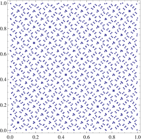
Figure 15: $2048$ Sobol’ points in the unit square generated using a method by [JoKu03].

This distribution property remains unchanged when lifting a digital net and elementary rectangles (now called spherical rectangles) to $\mathbb{S}^{2}$ using the area-preserving Lambert transformation of the map makers. These spherical digital nets are studied in [BrDi12] and [ABD12]. Of particular interest is that numerically they are comparable with maximal sum-of-distance points. It is conjectured that $\langle V_{-1}\rangle(\omega_{N}^{\mathrm{sphDN}})$ will approach the same limit as $v_{-1}(N)$ with the same rate of convergence as $N\to\infty$.

We tested for local concavity a sequence of $N$-point spherical digital nets formed by the first $N$ points of a Sobol’ sequence lifted to the sphere. For the implementation of the Sobol’ points we used [JoKu03]; cf. Fig. 15. The graph of $N\mapsto\langle V_{-1}\rangle(\omega_{N}^{\mathrm{sphDN}})$ (Fig. 16) shows an overall concave shape.

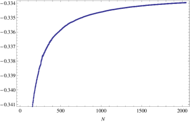
Figure 16: $\langle V_{-1}\rangle(\omega_{N}^{\mathrm{sphDN}})$ based on the $2048$ Sobol’ points given in Fig. 15.

Yet, some irregularities are clearly discernible in Fig. 16; in fact, the discrete second derivative of $N\mapsto\langle V_{-1}\rangle(\omega_{N}^{\mathrm{sphDN}})$ reveals that $N\mapsto\langle V_{-1}\rangle(\omega_{N}^{\mathrm{sphDN}})$ for this sequence of spherical digital nets is locally highly non-concave; see Fig. 17.

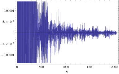
Figure 17: Discrete second derivative of $\langle V_{-1}\rangle(\omega_{N}^{\mathrm{sphDN}})$ based on the $2048$ Sobol’ points given in Fig. 15. The discrete points are joint by lines to guide the eye.

 

nerattini@fi.infn.it

brauchart@math.tugraz.at

miki@math.rutgers.edu

“Magic” numbers in Smale’s 7th problem:
Supplement

This supplementary section lists the standardized Riesz $s$-energy data used in the main part of our paper.

4.1 Tables for $s=-1$

Table 2: *

Putatively minimal average standardized Riesz pair-energy $v^{x}_{-1}(N)$ and its second derivative $\ddot{v}^{x}_{-1}$ converted from computer-experimental data ${\cal{E}}^{x}_{-1}(N)$ in [RSZ95]
$N$	$v^{x}_{-1}(N)$	$\ddot{v}^{x}_{-1}(N)$
2	-1.0000000000
3	-0.7320508077	-0.1688915465
4	-0.6329931618	-0.0342078637
5	-0.5681433797	-0.0280772524
6	-0.5313708499	-0.0068743336
7	-0.5014726538	-0.0096073663
8	-0.4811818239	-0.0042099548
9	-0.4651009489	-0.0031963792
10	-0.4522164530	-0.0020269265
11	-0.4413588837	-0.0025731588
12	-0.4330744732	-0.0004714806
13	-0.4252615432	-0.0014567068
14	-0.4189053200	-0.0007901741
15	-0.4133392709	-0.0007194468
16	-0.4084926687	-0.0005618514
17	-0.4042079178	-0.0004755958
18	-0.4003987627	-0.0003245148
19	-0.3969141224	-0.0004449970
20	-0.3938744790	-0.0002396557
21	-0.3910744914	-0.0002663080
22	-0.3885408118	-0.0001709545
23	-0.3861780867	-0.0002601472
24	-0.3840755088	-0.0001091965
25	-0.3820821274	-0.0001747639
26	-0.3802635100	-0.0001542742
27	-0.3785991667	-0.0000886587
28	-0.3770234821	-0.0000994882
29	-0.3755472858	-0.0001196462
30	-0.3741907356	-0.0000753432
31	-0.3729095285	-0.0001033183
32	-0.3717316398	-0.0000232543
33	-0.3705770053	-0.0000928414
34	-0.3695152123	-0.0000545753
35	-0.3685079946	-0.0000610507
36	-0.3675618275	-0.0000478945
37	-0.3666635549	-0.0000476311
38	-0.3658129134	-0.0000422886
39	-0.3650045606	-0.0000399725
40	-0.3642361802	-0.0000352382
41	-0.3635030381	-0.0000354383
42	-0.3628053343	-0.0000304398
43	-0.3621380703	-0.0000343435
44	-0.3615051498	-0.0000230366
45	-0.3608952658	-0.0000242521
46	-0.3603096340	-0.0000251566
47	-0.3597491588	-0.0000320904
48	-0.3592207739	-0.0000094516
49	-0.3587018407	-0.0000275106
50	-0.3582104181	-0.0000158895
51	-0.3577348849	-0.0000176294
52	-0.3572769812	-0.0000179846
53	-0.3568370621	-0.0000167784
54	-0.3564139214	-0.0000138648
55	-0.3560046454	-0.0000157930
56	-0.3556111625	-0.0000126576
57	-0.3552303372	-0.0000127819
58	-0.3548622938	-0.0000128192
59	-0.3545070695	-0.0000130118
60	-0.3541648570	-0.0000082593
61	-0.3538309038	-0.0000130841
62	-0.3535100347	-0.0000083204
63	-0.3531974859	-0.0000095653
64	-0.3528945024	-0.0000092839
65	-0.3526008028	-0.0000099603
66	-0.3523170635	-0.0000085228
67	-0.3520418471	-0.0000061002
68	-0.3517727307	-0.0000084551
69	-0.3515120695	-0.0000077804
70	-0.3512591888	-0.0000065818
71	-0.3510128898	-0.0000089700
72	-0.3507755608	-0.0000017464
73	-0.3505399783	-0.0000083169
74	-0.3503127126	-0.0000070610
75	-0.3500925079	-0.0000049921
76	-0.3498772953	-0.0000064646
77	-0.3496685474	-0.0000044272
78	-0.3494642267	-0.0000047166
79	-0.3492646225	-0.0000053979
80	-0.3490704162	-0.0000036243
81	-0.3488798341	-0.0000053146
82	-0.3486945667	-0.0000046236
83	-0.3485139228	-0.0000041813
84	-0.3483374603	-0.0000040455
85	-0.3481650433	-0.0000039518
86	-0.3479965781	-0.0000038940
87	-0.3478320068	-0.0000038600
88	-0.3476712956	-0.0000032965
89	-0.3475138808	-0.0000035676
90	-0.3473600336	-0.0000032498
91	-0.3472094363	-0.0000031976
92	-0.3470620364	-0.0000030669
93	-0.3469177035	-0.0000032350
94	-0.3467766057	-0.0000027273
95	-0.3466382351	-0.0000030607
96	-0.3465029252	-0.0000024914
97	-0.3463701068	-0.0000030062
98	-0.3462402945	-0.0000021599
99	-0.3461126421	-0.0000028725
100	-0.3459878622	-0.0000020284
101	-0.3458651107	-0.0000026513
102	-0.3457450106	-0.0000023406
103	-0.3456272511	-0.0000023449
104	-0.3455118366	-0.0000015587
105	-0.3453979807	-0.0000025700
106	-0.3452866950	-0.0000019386
107	-0.3451773478	-0.0000022877
108	-0.3450702883	-0.0000015216
109	-0.3449647504	-0.0000021798
110	-0.3448613924	-0.0000018916
111	-0.3447599259	-0.0000016306
112	-0.3446600899	-0.0000015411
113	-0.3445617950	-0.0000018275
114	-0.3444653276	-0.0000016283
115	-0.3443704885	-0.0000016236
116	-0.3442772731	-0.0000017758
117	-0.3441858334	-0.0000013487
118	-0.3440957425	-0.0000015893
119	-0.3440072409	-0.0000015063
120	-0.3439202456	-0.0000014235
121	-0.3438346739	-0.0000015652
122	-0.3437506673	-0.0000008439
123	-0.3436675047	-0.0000014344
124	-0.3435857765	-0.0000013062
125	-0.3435053545	-0.0000014107
126	-0.3434263433	-0.0000012300
127	-0.3433485620	-0.0000010363
128	-0.3432718170	-0.0000012992
129	-0.3431963713	-0.0000011613
130	-0.3431220868	-0.0000010782
131	-0.3430488805	-0.0000014789
132	-0.3429771532	-0.0000002910
133	-0.3429057168	-0.0000014821
134	-0.3428357625	-0.0000011364
135	-0.3427669446	-0.0000008849
136	-0.3426990116	-0.0000010022
137	-0.3426320808	-0.0000007288
138	-0.3425658788	-0.0000009612
139	-0.3425006380	-0.0000010152
140	-0.3424364125	-0.0000009987
141	-0.3423731856	-0.0000008186
142	-0.3423107773	-0.0000009224
143	-0.3422492915	-0.0000008783
144	-0.3421886840	-0.0000006861
145	-0.3421287625	-0.0000009504
146	-0.3420697915	-0.0000005912
147	-0.3420114117	-0.0000008435
148	-0.3419538754	-0.0000007333
149	-0.3418970724	-0.0000008899
150	-0.3418411593	-0.0000005652
151	-0.3417858113	-0.0000008084
152	-0.3417312717	-0.0000007905
153	-0.3416775227	-0.0000005462
154	-0.3416243199	-0.0000007311
155	-0.3415718481	-0.0000005965
156	-0.3415199729	-0.0000007574
157	-0.3414688550	-0.0000006272
158	-0.3414183644	-0.0000006462
159	-0.3413685199	-0.0000005827
160	-0.3413192581	-0.0000005710
161	-0.3412705674	-0.0000006268
162	-0.3412225034	-0.0000005491
163	-0.3411749886	-0.0000005855
164	-0.3411280593	-0.0000005656
165	-0.3410816956	-0.0000005625
166	-0.3410358944	-0.0000005158
167	-0.3409906091	-0.0000005912
168	-0.3409459150	-0.0000004328
169	-0.3409016537	-0.0000006121
170	-0.3408580044	-0.0000004603
171	-0.3408148156	-0.0000004770
172	-0.3407721037	-0.0000005051
173	-0.3407298968	-0.0000005265
174	-0.3406882164	-0.0000003733
175	-0.3406469094	-0.0000004704
176	-0.3406060727	-0.0000005030
177	-0.3405657391	-0.0000004271
178	-0.3405258325	-0.0000004416
179	-0.3404863676	-0.0000005073
180	-0.3404474099	-0.0000003502
181	-0.3404088025	-0.0000004928
182	-0.3403706878	-0.0000002503
183	-0.3403328233	-0.0000005234
184	-0.3402954823	-0.0000003383
185	-0.3402584796	-0.0000004666
186	-0.3402219435	-0.0000004336
187	-0.3401858409	-0.0000002152
188	-0.3401499536	-0.0000004637
189	-0.3401145299	-0.0000003905
190	-0.3400794967	-0.0000003512
191	-0.3400448147	-0.0000004582
192	-0.3400105908	-0.0000000862
193	-0.3399764531	-0.0000004471
194	-0.3399427626	-0.0000004414
195	-0.3399095134	-0.0000002415
196	-0.3398765058	-0.0000003723
197	-0.3398438704	-0.0000002997
198	-0.3398115348	-0.0000003509
199	-0.3397795500	-0.0000003349
200	-0.3397479002

4.2 Tables for $s=0$

Table 3: *

Putatively minimal average standardized Riesz pair-energy $v^{x}_{0}(N)$ and its second derivative $\ddot{v}^{x}_{0}$ converted from computer-experimental data ${\cal{E}}^{x}_{0}(N)$ in [RSZ95,Ca09]
$N$	$v^{x}_{0}(N)$	$\ddot{v}^{x}_{0}(N)$
2	-0.6931471806
3	-0.54930614433405	-0.08494951843776
4	-0.49041462650586	-0.01052760684652
5	-0.44205071552419	-0.02220150379344
6	-0.41588830833597	8.40980789335588E-05
7	-0.38964180306881	-0.00903390867908
8	-0.37242920648072	-0.00277652137846
9	-0.35799313127109	-0.00229013036125
10	-0.34584718642271	-0.00121657153476
11	-0.33491781310909	-0.0033773970446
12	-0.32736583684007	0.001009733962
13	-0.31880412660905	-0.0019313529543
14	-0.31217376933233	-0.00062683826669
15	-0.3061702503223	-0.00071787003732
16	-0.30088460134959	-0.00052653998475
17	-0.29612549236163	-0.00046555949713
18	-0.29183194287079	-0.0001802707487
19	-0.28771866412865	-0.00066371974506
20	-0.28426910513158	-0.00013717831788
21	-0.28095672445238	-0.0003037417766
22	-0.27794808554978	-7.39232856201699E-05
23	-0.27501336993281	-0.00043578332413
24	-0.27251443763996	2.3805380444275E-05
25	-0.26999169996667	-0.00025233942062
26	-0.26772130171399	-0.00022427146747
27	-0.26567517492879	-1.80666292328713E-05
28	-0.26364711477282	-9.17118141883222E-05
29	-0.26171076643103	-0.00020088190385
30	-0.2599752999931	-6.19871738598565E-05
31	-0.25830182072903	-0.00018389162935
32	-0.25681223309431	0.00011843935354
33	-0.25520420610606	-0.00019321886972
34	-0.25378939798752	-4.90378805957925E-05
35	-0.25242362774958	-9.14574502674514E-05
36	-0.2511493149619	-5.09700840284344E-05
37	-0.24992597225826	-6.00975463840858E-05
38	-0.248762727101	-5.12949955380482E-05
39	-0.24765077693927	-4.79551673250311E-05
40	-0.24658678194487	-3.72211580642046E-05
41	-0.24556000810854	-4.80799643073904E-05
42	-0.24458131423651	-3.35668470362871E-05
43	-0.24363618721152	-5.92585111488242E-05
44	-0.24275031869767	-7.97229394605692E-06
45	-0.24187242247778	-2.56166416358061E-05
46	-0.24102014289952	-3.72799285126846E-05
47	-0.24020514324977	-7.61240941284103E-05
48	-0.23946626769415	3.52976504339186E-05
49	-0.2386920944881	-6.46098671298889E-05
50	-0.23798253114917	-8.34470347785277E-06
51	-0.23728131251373	-2.04882748124635E-05
52	-0.23660058215309	-2.95202648709358E-05
53	-0.23594937205733	-2.36160936392393E-05
54	-0.23532177805521	-1.40962708229109E-05
55	-0.23470828032391	-2.5931202199847E-05
56	-0.23412071379481	-1.39709159995838E-05
57	-0.2335471181817	-1.6695091408836E-05
58	-0.23299021766001	-2.03062754731143E-05
59	-0.23245362341379	-2.26108284711313E-05
60	-0.23193963999605	7.18878297334413E-07
61	-0.2314249377	-2.7881591285861E-05
62	-0.23093811699524	-5.04737413728473E-06
63	-0.23045634366462	-1.27476168964025E-05
64	-0.22998731795089	-1.36433729289731E-05
65	-0.2295319356101	-1.78383549429839E-05
66	-0.22909439162424	-1.46188939495751E-05
67	-0.22867146653234	1.55185044292683E-06
68	-0.22824698958999	-1.55888787838065E-05
69	-0.22783810152643	-1.38738439675878E-05
70	-0.22744308730683	-6.93485401087601E-06
71	-0.22705500794125	-2.33475483877588E-05
72	-0.22669027612405	2.08645393496298E-05
73	-0.2263046797675	-2.20759411346805E-05
74	-0.22594115935209	-1.64016705273828E-05
75	-0.22559404060721	-3.30638960721608E-06
76	-0.22525022825193	-1.42299813379876E-05
77	-0.22492064587799	-2.00815429066137E-06
78	-0.22459307165834	-4.1880322580734E-06
79	-0.22426968547095	-1.04558366928464E-05
80	-0.22395675512025	4.70035913385791E-07
81	-0.22364335473364	-1.17868321321268E-05
82	-0.22334174117916	-8.75711084366571E-06
83	-0.22304888473553	-5.13968401155696E-06
84	-0.2227611679759	-5.62785486868389E-06
85	-0.22247907907115	-5.83387355199139E-06
86	-0.22220282403995	-6.58125936803255E-06
87	-0.22193315026811	-6.69772472819408E-06
88	-0.221670174221	-3.04605593015594E-06
89	-0.22141024422983	-6.19556534545151E-06
90	-0.221156509804	-4.28504674476748E-06
91	-0.22090706042491	-4.74832589339447E-06
92	-0.22066235937172	-4.02426048681792E-06
93	-0.22042168257901	-6.39575705141393E-06
94	-0.22018740154335	-2.6865068587234E-06
95	-0.21995580701456	-5.94847179991032E-06
96	-0.21973016095756	-2.35317439198357E-06
97	-0.21950686807496	-6.28182405801314E-06
98	-0.21928985701641	-8.8521900634686E-07
99	-0.21907373117687	-6.46345842683638E-06
100	-0.21886406879576	-7.93152682282416E-07
101	-0.21865519956733	-5.71565295034993E-06
102	-0.21845204599185	-3.77464931103355E-06
103	-0.21825266706568	-4.18706082880305E-06
104	-0.21805747520034	1.42216777929138E-06
105	-0.21786086116722	-7.1023501805878E-06
106	-0.21767134948428	-2.19010238333706E-06
107	-0.21748402790372	-5.3241145300531E-06
108	-0.21730203043769	2.69653456036467E-07
109	-0.21711976331821	-5.13758892570215E-06
110	-0.21694263378766	-3.57301988601622E-06
111	-0.21676907727699	-1.42480800854883E-06
112	-0.21659694557432	-8.29740063129636E-07
113	-0.21642564361173	-3.92481912320219E-06
114	-0.21625826646825	-2.41470970263613E-06
115	-0.21609330403448	-2.46277665663652E-06
116	-0.21593080437736	-4.2627595661926E-06
117	-0.21577256747981	-1.03527765454858E-06
118	-0.21561536585992	-3.10505495168534E-06
119	-0.21546126929497	-2.72592851491282E-06
120	-0.21530989865854	-2.43580446937508E-06
121	-0.21516096382658	-3.8488017444771E-06
122	-0.21501587779637	3.00937311131788E-06
123	-0.21486778239304	-3.51128303460735E-06
124	-0.21472319827275	-2.21756418575247E-06
125	-0.21458083171665	-3.45687768296687E-06
126	-0.21444192203822	-2.04205052439788E-06
127	-0.21430505441032	-4.39271462648883E-07
128	-0.21416862605389	-2.94498047931357E-06
129	-0.21403514267793	-1.952346087436E-06
130	-0.21390361164806	-1.51577687462767E-06
131	-0.21377359639507	-4.98986151248326E-06
132	-0.21364857100359	4.91205787697679E-06
133	-0.21351863355423	-5.43774509326189E-06
134	-0.21339413384996	-2.66422865552451E-06
135	-0.21327229837435	-6.31500497255688E-07
136	-0.21315109439924	-1.74302284844385E-06
137	-0.21303163344697	4.95917642923116E-07
138	-0.21291167657707	-1.79459218507816E-06
139	-0.21279351429934	-2.16703439157029E-06
140	-0.21267751905601	-2.73921437016211E-06
141	-0.21256426302705	-6.26072131720834E-07
142	-0.21245163307022	-2.13000696466792E-06
143	-0.21234113312036	-1.53863234181317E-06
144	-0.21223217180284	-2.44880969918482E-07
145	-0.21212345536628	-2.51754395819148E-06
146	-0.21201725647369	6.48949280507294E-07
147	-0.21191040863181	-1.89781145781831E-06
148	-0.2118054586014	-1.08596148842843E-06
149	-0.21170159453247	-2.47021583343887E-06
150	-0.21160020067937	4.70809362607127E-08
151	-0.21149875974534	-1.91372729155259E-06
152	-0.2113992325386	-1.9098988737476E-06
153	-0.21130161523074	2.90559403481883E-07
154	-0.21120370736347	-1.75255558348963E-06
155	-0.21110755205178	-4.45913007351972E-07
156	-0.2110118426531	-2.13449161656776E-06
157	-0.21091826774604	-9.05849323884489E-07
158	-0.2108255986883	-1.27272163832903E-06
159	-0.2107342023522	-6.79465345265751E-07
160	-0.21064348548145	-6.48182475859738E-07
161	-0.21055341679317	-1.35787387045561E-06
162	-0.21046470597876	-6.42757788021919E-07
163	-0.21037663792214	-1.10541287440258E-06
164	-0.21028967527839	-1.03610910762164E-06
165	-0.21020374874375	-9.70611329143001E-07
166	-0.21011879282045	-6.94936569872739E-07
167	-0.21003453183371	-1.51683901841726E-06
168	-0.20995178768599	3.98236263132734E-08
169	-0.20986900371464	-1.81203067378677E-06
170	-0.20978803177396	-4.81552880238212E-07
171	-0.20970754138617	-6.28672096575356E-07
172	-0.20962767967047	-1.00642611994273E-06
173	-0.2095488243809	-1.16785260270702E-06
174	-0.20947113694392	-2.97605704802084E-08
175	-0.20939347926752	-7.39769662222445E-07
176	-0.20931656136078	-1.31451110071956E-06
177	-0.20924095796514	-5.50239363683591E-07
178	-0.20916590480886	-7.50620530370893E-07
179	-0.20909160227312	-1.42310080628039E-06
180	-0.20901872283818	-1.0896361599122E-07
181	-0.20894595236685	-1.42841684058759E-06
182	-0.20887461031237	1.0368942854333E-06
183	-0.2088022313636	-1.96770331067908E-06
184	-0.20873182011814	-5.79824303015286E-08
185	-0.20866146685511	-1.47193601873763E-06
186	-0.2085925855281	-1.17488648110342E-06
187	-0.20852487908757	1.14936697975798E-06
188	-0.20845602328007	-1.62552704796592E-06
189	-0.20838879299961	-8.99850945978997E-07
190	-0.20832246257009	-5.7871458888914E-07
191	-0.20825671085517	-1.55592193121223E-06
192	-0.20819251506217	2.22030766108827E-06
193	-0.20812609896152	-1.68921007370759E-06
194	-0.20806137207094	-1.70547896297113E-06
195	-0.20799835065932	3.95655705892617E-07
196	-0.20793493359199	-1.01998206419873E-06
197	-0.20787253650673	-1.7647982364366E-07
198	-0.2078103159013	-9.81940776911827E-07
199	-0.20774907723664	-7.58389227834E-07
200	-0.20768859696121

4.3 Tables for $s=1$

Table 4: *

Putatively minimal average standardized Riesz pair-energy $v^{x}_{1}(N)$ and its second derivative $\ddot{v}^{x}_{1}$ converted from computer-experimental data ${\cal{E}}^{x}_{1}(N)$ in [RSZ95,Ca09]
$N$	$v^{x}_{1}(N)$	$\ddot{v}^{x}_{1}(N)$
2	-0.5
3	-0.42264973066667	-0.04232810533333
4	-0.38762756666667	7.45526666665608E-05
5	-0.35253085	-0.01688044
6	-0.33431457333333	0.00433531571429
7	-0.31176298095238	-0.00809975785714
8	-0.29731114642857	-0.00158550753968
9	-0.28444481944444	-0.00137818531746
10	-0.27295667777778	-0.00041418207071
11	-0.26188271818182	-0.00426316414141
12	-0.25507192272727	0.00278972470862
13	-0.2454714025641	-0.00252072968698
14	-0.23839161208791	-0.00040013934066
15	-0.23171196095238	-0.00070389601648
16	-0.22573620583333	-0.00045716105042
17	-0.22021761176471	-0.00043518230392
18	-0.2151342	4.76747850017833E-05
19	-0.21000311345029	-0.0010144555731
20	-0.20588648247368	6.32914970759568E-05
21	-0.20170656	-0.00036281636979
22	-0.1978894538961	0.00012053221909
23	-0.19395181557312	-0.00075729358319
24	-0.19077147083333	0.00030032709354
25	-0.187290799	-0.00039502261795
26	-0.18420514978462	-0.00035453068433
27	-0.18147403125356	0.00014910944208
28	-0.17859380328042	-6.36662690692846E-05
29	-0.17577724157635	-0.00036358242656
30	-0.17332426229885	-3.01405055350701E-05
31	-0.17090142352688	-0.00034949054751
32	-0.16882807530242	0.00047453285447
33	-0.16628019422348	-0.00043015872711
34	-0.16416247187166	-2.26916734467064E-05
35	-0.16206744119328	-0.00015075078669
36	-0.16012316130159	-5.10168934061417E-05
37	-0.1582298983033	-8.08560605566333E-05
38	-0.15641749136558	-6.56186490742838E-05
39	-0.15467070307692	-5.64969681400296E-05
40	-0.15298041175641	-3.09230519075498E-05
41	-0.1513210434878	-7.33915171534649E-05
42	-0.14973506673635	-3.38043008132338E-05
43	-0.14818289428571	-0.0001195286089
44	-0.14675025044397	5.33652486994773E-05
45	-0.14526424135354	-2.16579398023553E-05
46	-0.1437998902029	-7.03160078679987E-05
47	-0.14240585506013	-0.00019965584505
48	-0.14121147576241	0.00018476878612
49	-0.13983232767857	-0.00017350225833
50	-0.13862668185306	2.44009844140303E-05
51	-0.13739663504314	-1.82048889588726E-05
52	-0.13618479312217	-6.16711355130306E-05
53	-0.13503462233672	-3.48533194521883E-05
54	-0.13391930487072	-8.99523501085575E-06
55	-0.13281298263973	-4.98686302196072E-05
56	-0.13175652903896	-1.21869364950733E-05
57	-0.13071226237469	-2.45326380451383E-05
58	-0.12969252834846	-3.94585825060911E-05
59	-0.12871225290473	-4.74570135655661E-05
60	-0.12777943447458	3.88729843092683E-05
61	-0.12680774306011	-7.11879630302947E-05
62	-0.12590723960867	9.13323864926152E-06
63	-0.12499760291859	-1.78978935229113E-05
64	-0.12410586412202	-2.2432241846948E-05
65	-0.12323655756731	-3.76322974317E-05
66	-0.12240488331002	-3.57007573017487E-05
67	-0.12160890981004	3.8002925510261E-05
68	-0.12077493338455	-3.62454151990876E-05
69	-0.11997720237425	-3.3405841008749E-05
70	-0.11921287720497	-2.18984359168228E-06
71	-0.11845074187928	-7.30558212219679E-05
72	-0.1177616623748	0.00011439556059
73	-0.11695818730974	-7.1506992641468E-05
74	-0.11622621923732	-4.82032351019068E-05
75	-0.1155424544	7.76740127672593E-06
76	-0.1148509221614	-4.08314203234061E-05
77	-0.11420022134313	1.18830190299901E-05
78	-0.11353763750583	5.32224366234235E-06
79	-0.11286973142486	-2.73278269893318E-05
80	-0.11222915317089	2.15470341941026E-05
81	-0.11156702788272	-3.4671241648021E-05
82	-0.11093957383619	-2.33227845273243E-05
83	-0.1103354425742	-3.30589089370115E-06
84	-0.1097346172031	-8.66112598618685E-06
85	-0.10914245295798	-1.01474813861691E-05
86	-0.10856043619425	-1.38954558682736E-05
87	-0.10799231488639	-1.56714266911218E-05
88	-0.10743986500522	2.58841823319589E-06
89	-0.10688482670582	-1.4475583592799E-05
90	-0.10634426399001	-4.9191604736265E-06
91	-0.10580862043468	-8.52425778341548E-06
92	-0.10528150113712	-3.83732358921751E-06
93	-0.10475821916316	-1.82612505194024E-05
94	-0.10425319843972	1.63249118823039E-06
95	-0.10374654522508	-1.58075377939548E-05
96	-0.10325569954825	1.45172793653003E-06
97	-0.10276340214347	-1.74573989013549E-05
98	-0.1022885621376	7.73638239381924E-06
99	-0.10180598574933	-1.98968348971151E-05
100	-0.10134330619596	7.36955150049123E-06
101	-0.10087325709109	-1.67947511141575E-05
102	-0.10042000273733	-7.24422445752548E-06
103	-0.09997399260803	-9.6346329160335E-06
104	-0.09953761711165	1.7109311238328E-05
105	-0.09908413230403	-2.44116769972935E-05
106	-0.09865505917341	-1.21414942477749E-06
107	-0.09822720019221	-1.76356269994127E-05
108	-0.09781697683801	1.21017542786817E-05
109	-0.09739465172953	-1.69487434211746E-05
110	-0.09698927536447	-1.0169044812991E-05
111	-0.09659406804423	2.73497269465128E-06
112	-0.09619612575129	5.67050480826392E-06
113	-0.09579251295354	-1.21909542836196E-05
114	-0.09540109111008	-4.6273344553871E-06
115	-0.09501429660107	-2.84369804537388E-06
116	-0.0946303457901	-1.49597836047732E-05
117	-0.09426135476275	2.31995587263167E-06
118	-0.09389004377952	-8.21244228454976E-06
119	-0.09352694523857	-7.53635839867428E-06
120	-0.09317138305602	-4.84722845350838E-06
121	-0.09282066810193	-1.41954417874901E-05
122	-0.09248414858962	2.81073086896289E-05
123	-0.09211952176863	-1.40567714890238E-05
124	-0.09176895171912	-4.42297296898708E-06
125	-0.09142280464258	-1.2964672687743E-05
126	-0.09108962223873	-4.77692552514064E-06
127	-0.0907612167604	5.57740781781391E-06
128	-0.09042723387426	-1.00291390614515E-05
129	-0.09010328012718	-3.93194906056493E-06
130	-0.08978325832916	-1.805519360909E-06
131	-0.0894650420505	-2.21144548554486E-05
132	-0.08916894022669	3.47446343774704E-05
133	-0.08883809376851	-2.49352516719092E-05
134	-0.088532182562	-9.27458259558644E-06
135	-0.08823554593809	2.44989587205868E-06
136	-0.0879364594183	-3.83633506273462E-06
137	-0.08764120923358	9.28179083925507E-06
138	-0.08733667725801	-4.96691127305215E-06
139	-0.08703711219372	-6.48071846010012E-06
140	-0.08674402784789	-1.1533783651152E-05
141	-0.08646247728571	2.88057330044555E-06
142	-0.08617804615023	-8.10357186920019E-06
143	-0.08590171858662	-2.83406828316402E-06
144	-0.0856282250913	3.08765248391296E-06
145	-0.08535164394349	-9.31835028550321E-06
146	-0.08508438114596	9.77312152317111E-06
147	-0.08480734522691	-6.73755093349993E-06
148	-0.0845370468588	-1.35350460139794E-06
149	-0.08426810199528	-1.01102776257633E-05
150	-0.0840092674094	3.98419392733107E-06
151	-0.08374644862958	-6.47185117563787E-06
152	-0.08349010170094	-6.46295731676627E-06
153	-0.08324021772962	6.92158106085916E-06
154	-0.08298341217723	-6.97592395515478E-06
155	-0.08273358254881	2.22367802815704E-06
156	-0.08248152924235	-9.37420619473439E-06
157	-0.08223885014209	-9.11422094795888E-07
158	-0.08199708246392	-3.78393568656321E-06
159	-0.08175909872144	2.66358675782286E-07
160	-0.08152084862028	3.57793971339504E-07
161	-0.08128224072516	-4.5739171544712E-06
162	-0.08104820674718	1.95129278290906E-07
163	-0.08081397763993	-3.06567351604503E-06
164	-0.08058281420619	-2.78741157611062E-06
165	-0.08035443818404	-1.78951245766168E-06
166	-0.08012785167433	-1.38040567321251E-06
167	-0.07990264557031	-5.14734082346369E-06
168	-0.0796825868071	3.97994090828302E-06
169	-0.07945854810299	-8.01907032266236E-06
170	-0.0792425284692	4.29077579244819E-07
171	-0.07902607975783	-5.07074718991696E-07
172	-0.07881013812118	-2.70880987029987E-06
173	-0.07859690529439	-4.00328217031731E-06
174	-0.07838767574978	3.16258809651693E-06
175	-0.07817528361708	-1.08412407107128E-06
176	-0.07796397560844	-5.57936359946165E-06
177	-0.07775824696341	-3.57159952613095E-07
178	-0.07755287547832	-1.40102088563854E-06
179	-0.07734890501412	-5.90793734966955E-06
180	-0.07715084248727	1.72040057400125E-06
181	-0.07695105955985	-6.01734425598188E-06
182	-0.07675729397669	1.07493765258981E-05
183	-0.07655277901699	-1.06424341453915E-05
184	-0.07635890649145	2.87615567673427E-06
185	-0.07616215781022	-6.84096980885229E-06
186	-0.07597225009881	-5.41068488502106E-06
187	-0.07578775307228	1.00531148125027E-05
188	-0.07559320293094	-5.38082179846189E-06
189	-0.07540403361139	-4.94420160701559E-06
190	-0.07521980849346	-1.49464266796517E-06
191	-0.07503707801819	-7.21515014479035E-06
192	-0.07486156269306	1.87730199249225E-05
193	-0.07466727434801	-9.35273588464902E-06
194	-0.07448233873885	-9.26861601924234E-06
195	-0.0743066717457	5.44473581409743E-06
196	-0.07412556001675	-4.57468066927813E-06
197	-0.07394902296846	2.40835261167138E-06
198	-0.07377007756755	-5.0053065725475E-06
199	-0.07359613747322	-2.79168994843371E-06
200	-0.07342501145829

4.4 Tables for $s=2$

Table 5: *

Putatively minimal average standardized Riesz pair-energy $v^{x}_{2}(N)$ and its second derivative $\ddot{v}^{x}_{2}$ converted from computer-experimental data ${\cal{E}}^{x}_{2}(N)$ in [Ca09,Cec]
$N$	$v^{x}_{2}(N)$	$\ddot{v}^{x}_{2}(N)$
2	-0.375
3	-0.33333333333333	-0.02083333333333
4	-0.3125	0.00416666666667
5	-0.2875	-0.0125
6	-0.275	0.00654761904762
7	-0.25595238095238	-0.00708111160256
8	-0.24398587350732	-0.00057967860454
9	-0.23259904466681	-0.00055045392804
10	-0.22176266975433	0.00033285517504
11	-0.21059343966682	-0.00512124496615
12	-0.20454545454545	0.00473662955787
13	-0.19376083986622	-0.00317098031643
14	-0.18614720550341	-0.00010364440555
15	-0.17863721554614	-0.00065340344862
16	-0.1717806290375	-0.00034316587478
17	-0.16526720840364	-0.00034854790081
18	-0.15910233567059	0.00038063150976
19	-0.15255683142778	-0.00152293973609
20	-0.14753426692105	0.00042866131909
21	-0.14208304109524	-0.00045522879984
22	-0.13708704406926	0.00047783137135
23	-0.13161321567194	-0.00129097866742
24	-0.12743036594203	0.00082264497879
25	-0.12242487123333	-0.00063117898305
26	-0.11805055550769	-0.00057104766809
27	-0.11424728745014	0.00049490776561
28	-0.10994911162698	5.65472008196011E-06
29	-0.10564528108374	-0.00065437631007
30	-0.10199582685057	4.62317141797786E-05
31	-0.09830014090323	-0.00065764181832
32	-0.09526209677419	0.0012504149463
33	-0.09097363769886	-0.0009251275975
34	-0.08761030622103	5.91024322797451E-05
35	-0.08418787231092	-0.0002549928849
36	-0.08102043128571	-3.31672244807679E-05
37	-0.07788615748498	-0.00011337017065
38	-0.07486525385491	-7.51279263169202E-05
39	-0.07191947815115	-5.87632577415675E-05
40	-0.06903246570513	2.86269813359885E-06
41	-0.06614259056098	-0.00011825042522
42	-0.06337096584204	-1.97694361344092E-05
43	-0.06061911055925	-0.00025016977112
44	-0.05811742504757	0.00024097656619
45	-0.0553747629697	5.2138628396925E-06
46	-0.05262688702899	-0.00015625953615
47	-0.05003527062442	-0.00050422672429
48	-0.04794788094415	0.00060527859806
49	-0.04525521266582	-0.00045806519211
50	-0.04302060957959	0.00013046977964
51	-0.04065553671373	9.33868571739715E-06
52	-0.03828112516214	-0.00014110705345
53	-0.03604782066401	-4.82038341302893E-05
54	-0.03386272	1.7415376398322E-05
55	-0.0316602039596	-0.00010261269444
56	-0.02956030061364	7.02587356660178E-06
57	-0.02745337139411	-4.07512525181786E-05
58	-0.0253871934271	-8.35262289764493E-05
59	-0.02340454168907	-0.00010505587664
60	-0.02152694582768	0.00016769257832
61	-0.01948165738798	-0.00018739457367
62	-0.01762376352195	5.47408259087834E-05
63	-0.01571112883001	-2.05467919953128E-05
64	-0.01381904093006	-3.61050203668833E-05
65	-0.01196305805048	-8.62239386549835E-05
66	-0.01019329910956	-9.33649851432294E-05
67	-0.00851690515378	0.00016530091924
68	-0.00667521027875	-9.06002249997928E-05
69	-0.00492411562873	-9.00175016249616E-05
70	-0.00326303848033	2.51906377677358E-05
71	-0.00157677069417	-0.00022621951962
72	-0.00011672242762	0.00043654750963
73	0.00177987334855	-0.00023064867119
74	0.00344582045354	-0.00014405338374
75	0.00496771417477	5.35525706528706E-05
76	0.00654316046667	-0.00012329288809
77	0.00799531387047	6.57277856631611E-05
78	0.00951319505994	5.75274490662858E-05
79	0.01108860369847	-8.13307784647277E-05
80	0.01258268155854	0.00010413254126
81	0.01418089195988	-0.00010840762017
82	0.01567069474104	-6.89680790688652E-05
83	0.01709152944314	1.4776226251012E-05
84	0.01852714037149	-1.34604538951644E-05
85	0.01994929084594	-1.85602437833277E-05
86	0.02135288107661	-3.04430634913144E-05
87	0.02272602824379	-4.26087560516653E-05
88	0.02405656665491	3.22744308983713E-05
89	0.02541937949694	-3.88368458263955E-05
90	0.02674335549313	5.70681608413892E-07
91	0.02806790217094	-1.67719447810022E-05
92	0.02937567690397	6.46410634697059E-06
93	0.03068991574334	-5.95216588944458E-05
94	0.03194463292382	2.69131375872922E-05
95	0.03322626324188	-4.76866915255503E-05
96	0.03446020686842	2.42741077024489E-05
97	0.03571842460266	-5.37049783949639E-05
98	0.03692293735851	4.71981375491648E-05
99	0.03817464825191	-6.65380220707945E-05
100	0.03935982112323	4.45316430658371E-05
101	0.04058952563762	-5.40295618385311E-05
102	0.04176520059018	-1.36110072259665E-05
103	0.0429272645355	-2.43687086123323E-05
104	0.04406495977222	8.21308857559266E-05
105	0.04528478589469	-8.43384376443268E-05
106	0.04642027357951	7.58413329604579E-06
107	0.04756334539764	-6.36426596846151E-05
108	0.04864277455607	6.80430404995658E-05
109	0.04979024675501	-6.0937156617924E-05
110	0.05087678179733	-3.41841983727553E-05
111	0.05192913264128	2.75757120087317E-05
112	0.05300905919723	3.81404359711679E-05
113	0.05412712618916	-4.13185040168962E-05
114	0.05520387467707	-1.00696020491897E-05
115	0.05627055356293	2.50510293475781E-06
116	0.05733973755172	-5.52473082764404E-05
117	0.05835367423224	1.96518802271228E-05
118	0.05938726279299	-2.40406828896367E-05
119	0.06039681067084	-2.54941215299676E-05
120	0.06138086442717	-9.83905057683199E-06
121	0.06235507913292	-5.56362475571115E-05
122	0.06327365759111	0.00015092856218
123	0.06434316461149	-6.28610588254697E-05
124	0.06534981057304	-6.36578749368955E-06
125	0.0663500907471	-5.3654187820551E-05
126	0.06729671673333	-1.44415809621989E-05
127	0.06822890113861	4.04506944298166E-05
128	0.06920153623831	-3.86387829048873E-05
129	0.07013553255511	-7.76854454043185E-06
130	0.07106176032737	1.58402603134267E-06
131	0.07198957212566	-9.64878483089571E-05
132	0.07282089607564	0.00017520935863
133	0.07382742938426	-0.00011025383135
134	0.07472370886152	-3.57454742164753E-05
135	0.07558424286457	2.04098796637853E-05
136	0.07646518674728	-9.11528595537447E-06
137	0.07733701534403	5.55155963970488E-05
138	0.07826435953718	-1.70098308470701E-05
139	0.07917469389949	-2.21642751551121E-05
140	0.08006286398664	-5.10005236372679E-05
141	0.08090003355015	2.56656072422645E-05
142	0.08176286872091	-3.56716332161611E-05
143	0.08259003225845	-2.4199563383176E-06
144	0.08341477583965	1.98712142105428E-05
145	0.08425939063506	-3.62580133689283E-05
146	0.0850677474171	5.89034939901811E-05
147	0.08593500769313	-2.91501253510962E-05
148	0.08677311784381	4.31646088372428E-06
149	0.08761554445538	-4.60305810371375E-05
150	0.08841194048591	2.44734968111171E-05
151	0.08923281001325	-2.45391136058926E-05
152	0.09002914042698	-2.40588137072617E-05
153	0.090801412027	4.39663874003404E-05
154	0.09161765001443	-3.16951149688105E-05
155	0.09240219288689	1.99327377604641E-05
156	0.09320666849711	-4.35444629491855E-05
157	0.09396759964437	3.22203751190742E-06
158	0.09473175282915	-1.37141092296789E-05
159	0.09548219190471	8.79071510573315E-06
160	0.09624142169536	8.82254154399575E-06
161	0.09700947402756	-1.80071166065998E-05
162	0.09775951924316	7.78953806879201E-06
163	0.09851735399682	-1.04178560480506E-05
164	0.09926477089443	-9.04683195968037E-06
165	0.10000314096009	-1.11980741579476E-06
166	0.10074039121833	-5.4279234323884E-06
167	0.10147221355313	-1.84494793301626E-05
168	0.10218558640861	2.71187804316009E-05
169	0.10292607804452	-3.81989052800069E-05
170	0.10362837077515	9.0726758542603E-06
171	0.10433973618163	2.24229295586742E-06
172	0.10505334388107	-9.13906908106554E-06
173	0.10575781251143	-1.54236575632405E-05
174	0.10644685748422	2.26676546440929E-05
175	0.10715857011166	5.90782331832962E-07
176	0.10787087352143	-2.63275045164768E-05
177	0.10855684942668	2.3344125574809E-06
178	0.10924515974449	-1.09400399017634E-06
179	0.10993237605831	-2.66541589132308E-05
180	0.11059293821322	1.15582399126124E-05
181	0.11126505860804	-2.67373326537923E-05
182	0.11191044167021	6.69827539641066E-05
183	0.11262280748634	-5.68771647287969E-05
184	0.11327829613774	2.23036620916606E-05
185	0.11395608845123	-3.30450971889329E-05
186	0.11460083566754	-2.81054961135396E-05
187	0.11521747738773	6.40038727942605E-05
188	0.11589812298071	-2.56804432821056E-05
189	0.11655308813042	-2.45519164336905E-05
190	0.11718350136369	-5.99227262465529E-06
191	0.11780792232433	-3.29110832968382E-05
192	0.11839943220168	0.00011409688875
193	0.11910503896778	-5.2031424011334E-05
194	0.11975861430987	-4.86327746073156E-05
195	0.12036355687735	3.55299256605823E-05
196	0.12100402937049	-2.22191655023796E-05
197	0.12162228269813	2.08701389292631E-05
198	0.12226140616469	-2.72087952620792E-05
199	0.122873320836	-1.23590826804909E-05
200	0.12347287642462

4.5 Tables for $s=3$

Table 6: *

Putatively minimal average standardized Riesz pair-energy $v^{x}_{3}(N)$ and its second derivative $\ddot{v}^{x}_{2}$ converted from computer-experimental data ${\cal{E}}^{x}_{3}(N)$ in [Ca09,Cec]
$N$	$v^{x}_{3}(N)$	$\ddot{v}^{x}_{3}(N)$
2	-0.29166666666667
3	-0.2691833	-0.01008684444444
4	-0.25678677777778	0.00517927555556
5	-0.23921098	-0.00908391333333
6	-0.23071909555556	0.00737168095238
7	-0.21485553015873	-0.00608242214286
8	-0.20507438690476	0.00023825013228
9	-0.19505499351852	0.00015172161376
10	-0.18488387851852	0.00099516412458
11	-0.17371759939394	-0.00588602670034
12	-0.1684373469697	0.00674183941725
13	-0.15641525512821	-0.00383768616384
14	-0.14823084945055	0.00025603361416
15	-0.13979041015873	-0.00053858996642
16	-0.13188856083333	-0.00019836079599
17	-0.12418507230392	-0.00015616045207
18	-0.11663774422658	0.00084523349817
19	-0.10824518265107	-0.00222980981917
20	-0.10208243089474	0.00104769691618
21	-0.09487198222222	-0.00060346509387
22	-0.08826499864358	0.00109302169208
23	-0.08056499337286	-0.00214217918047
24	-0.07500716728261	0.00175267115902
25	-0.06769667003333	-0.00100596925697
26	-0.06139214204103	-0.00091503559041
27	-0.05600264963913	0.00115103266051
28	-0.04946212457672	0.00014840648476
29	-0.04277319302956	-0.00114977201952
30	-0.03723403350192	0.00022188482015
31	-0.03147298915412	-0.00120635483749
32	-0.02691829964382	0.00280037730523
33	-0.01956323282828	-0.00188481440318
34	-0.01409298041592	0.00025763185791
35	-0.00836509614566	-0.00042633428334
36	-0.00306354615873	4.2583899529677E-05
37	0.00228058772773	-0.00017826218792
38	0.00744645942627	-3.56287001576465E-05
39	0.01257670242465	-4.8327427307978E-05
40	0.01765861799573	0.00010472418523
41	0.02284525775203	-0.00019360091523
42	0.02783829659311	3.51409925407678E-05
43	0.03286647642673	-0.00051981849079
44	0.03737483776956	0.00073780197852
45	0.04262100109091	9.21431368521367E-05
46	0.04795930754911	-0.00035398032246
47	0.05294363368486	-0.00121438817462
48	0.05671357164598	0.0016791584031
49	0.0621626680102	-0.00115421019211
50	0.06645755418231	0.0004243123044
51	0.07117675265882	0.00011958393757
52	0.0760155350729	-0.00032546670807
53	0.08052885077891	-5.61197833050947E-05
54	0.08498604670161	0.00011398397277
55	0.08955722659708	-0.00021864014624
56	0.09390976634632	8.3101051475451E-05
57	0.09834540714703	-7.21014484539179E-05
58	0.10270894649929	-0.00018594031678
59	0.10688654553478	-0.00022206671527
60	0.11084207785499	0.00054714300148
61	0.11534475317668	-0.00048653601821
62	0.11936089248017	0.0001802723365
63	0.12355730412016	4.3263347625222E-06
64	0.12775804209491	-5.15173597218366E-05
65	0.13190726270994	-0.00019978950367
66	0.13585669382129	-0.00024366441101
67	0.13956246052163	0.00055550923398
68	0.14382373645596	-0.00022708593816
69	0.14785792645212	-0.00024535484855
70	0.15164676159972	0.00013100204677
71	0.1555665987941	-0.00066592521513
72	0.15882051077334	0.00143510479688
73	0.16350952754947	-0.00070960675555
74	0.16748893757004	-0.0004133927858
75	0.1710549548048	0.00021124809025
76	0.17483222012982	-0.00036314952753
77	0.17824633592732	0.00024507688991
78	0.18190552861472	0.00026234373412
79	0.18582706503624	-0.00024594046304
80	0.18950266099473	0.0003869692721
81	0.19356522622531	-0.00033831314012
82	0.19728947831577	-0.00018858494634
83	0.20082514545989	8.91076541672253E-05
84	0.20444992025818	-1.67607390024194E-05
85	0.20805793431746	-2.94907807580069E-05
86	0.21163645759599	-6.9839552229306E-05
87	0.21514514132228	-0.00011657445907
88	0.21853725058952	0.00014983699889
89	0.22207919685563	-0.00010861201564
90	0.22551253110612	3.5637838353475E-05
91	0.22898150319495	-3.25853849199031E-05
92	0.23241788989887	6.12636395398991E-05
93	0.23591554024233	-0.00019466580045
94	0.23921852478533	0.00013426682695
95	0.24265577615528	-0.00014976206544
96	0.2459432654598	0.00012888508606
97	0.24935963985037	-0.00016969671728
98	0.25260631752367	0.00020021463468
99	0.25605320983165	-0.00022261889586
100	0.25927748324377	0.00019225679823
101	0.26269401345413	-0.0001765310158
102	0.26593401264868	-1.82619993290833E-05
103	0.2691557498439	-6.26353506716915E-05
104	0.27231485168845	0.00032375670265
105	0.27579771023565	-0.00028172388738
106	0.27899884489548	5.15872806469697E-05
107	0.28225156683595	-0.0002268305527
108	0.28527745822372	0.00029510069715
109	0.28859845030864	-0.00021822102298
110	0.29170122137059	-0.00011385262691
111	0.29469013980562	0.00013750345979
112	0.29781656170045	0.00017153871193
113	0.30111452230721	-0.00013796399609
114	0.30427451891787	-2.08736037944357E-05
115	0.30741364192474	3.81762178164879E-05
116	0.31059094114943	-0.00020228574694
117	0.31356595462717	9.62420288364019E-05
118	0.31663721013376	-7.14383650260997E-05
119	0.31963702727532	-8.89885952134462E-05
120	0.32254785582166	-1.67171852707981E-05
121	0.32544196718274	-0.00021083099063
122	0.32812524755318	0.00066944307554
123	0.33147797099916	-0.00026854220281
124	0.33456215224233	6.41573772408588E-06
125	0.33765274922323	-0.00021233852158
126	0.34053100768254	-4.69055694251042E-05
127	0.34336236057243	0.00020195688012
128	0.34639567034244	-0.00014974616017
129	0.34927923395228	-1.15512512439686E-05
130	0.35215124631087	2.82856096472939E-05
131	0.35505154427912	-0.00039695938939
132	0.35755488285797	0.00076984175335
133	0.36082806319017	-0.00045767072882
134	0.36364357279355	-0.00013655471829
135	0.36632252767864	0.00010516120896
136	0.36910664377269	-2.1922376047645E-05
137	0.3718688374907	0.00026705962525
138	0.37489809083395	-6.26094637574681E-05
139	0.37786473471345	-8.1069922507504E-05
140	0.38075030867044	-0.0002112555359
141	0.38342462709152	0.00013826251456
142	0.38623720802717	-0.00015317580086
143	0.38889661316196	1.6459216857001E-05
144	0.3915724775136	9.38702608777042E-05
145	0.39434221212612	-0.00013845644325
146	0.39697349029539	0.00028687611118
147	0.39989164457584	-0.00012404268941
148	0.40268575616688	4.37222420768268E-05
149	0.40552359	-0.00020117788711
150	0.40816024594601	0.00012163092122
151	0.41091853281325	-9.63273991968494E-05
152	0.41358049228128	-8.99460587460155E-05
153	0.41615250569057	0.00021986323384
154	0.4189443823337	-0.00013852647383
155	0.421597732503	0.00011045146252
156	0.42436153413482	-0.00019248156826
157	0.42693285419838	3.22672514103672E-05
158	0.42953644151334	-5.16714714109967E-05
159	0.4320883573569	5.73596687816202E-05
160	0.43469763286923	5.59946091118757E-05
161	0.43736290299068	-7.2164600769975E-05
162	0.43995600851136	5.09445660059615E-05
163	0.44260005859805	-3.7249956115426E-05
164	0.44520685872861	-3.09464943156201E-05
165	0.44778271236487	1.37567833498053E-05
166	0.45037232278447	-2.46402004429602E-05
167	0.45293729300363	-6.64396903324871E-05
168	0.45543582353246	0.0001430025502
169	0.45807735661149	-0.00017571816366
170	0.46054317152686	6.17658464966975E-05
171	0.46307075228873	2.14594050894634E-05
172	0.46561979245569	-3.44765501449906E-05
173	0.4681343560725	-6.01711188982224E-05
174	0.47058874857042	0.0001229489921
175	0.47316609006043	1.79884140644182E-05
176	0.4757614199645	-0.00011874172421
177	0.47823800814437	1.42237316299032E-05
178	0.48072882005586	1.41239276478244E-05
179	0.48323375589501	-0.00011768412521
180	0.48562100760894	5.7555300414458E-05
181	0.48806581462329	-0.0001156824188
182	0.49039493921883	0.00035225004739
183	0.49307631386177	-0.00028312093798
184	0.49547456756672	0.00012752974517
185	0.49800035101684	-0.00015216603628
186	0.50037396843069	-0.00014008695507
187	0.50260749888946	0.000342797297
188	0.50518382664524	-0.00012066947756
189	0.50763948492345	-0.00011670478822
190	0.50997843841344	-3.32734698882398E-05
191	0.51228411843354	-0.0001337348389
192	0.51445606361475	0.00059785481804
193	0.51722586361399	-0.00027187826327
194	0.51972378534996	-0.00023549816973
195	0.5219862089162	0.00019285863599
196	0.52444149111844	-0.0001048140132
197	0.52679195930747	0.00012282712877
198	0.52926525462527	-0.00013765031158
199	0.53160089963149	-5.55293841086879E-05
200	0.5338810152536

References

- [ABD12] Aistleitner, Ch., Brauchart, J.S., and Dick, J., “Point sets on the sphere with small spherical cap discrepancy,” Discrete Comput. Geom. 48:4, 990–1024 (2012).
- [Aetal97] Altschuler, E.L., Williams, T.J., Ratner, E.R., Tipton, R., Stong, R., Dowla, F., and Wooten, F.: “Possible global minimum lattice configurations for Thomson’s problem of charges on the sphere,” Phys. Rev. Lett. 78:2681–2685 (1997).
- [ABS11] Armentano, D., Beltrán, C., and Shub, M., “Minimizing the discrete logarithmic energy on the sphere: The role of random polynomials,” Trans. Amer. Math. Soc. 363:2955–2965 (2011).
- [AtSu03] Atiyah, M., and Sutcliffe, P., “Polyhedra in physics, chemistry, and geometry,” Milan J. Math. 71:33–58 (2003).
- [BaVa08] Bachoc, C., and Vallentin, F., “New upper bounds for kissing numbers from semidefinite programming,” J. Amer. Math. Soc. 21:3, 909–924 (2008).
- [Bec84] Beck, J., “Sums of distances between points on a sphere — an application of the theory of irregularities of distribution to discrete geometry,” Mathematica 31:33–41 (1984).
- [Bel13a] Beltran, C., “Harmonic properties of the logarithmic potential and the computability of elliptic Fekete points,” Constr. Approx. 37:135–165 (2013).
- [Bel13b] Beltran, C., “The state of the art in Smale’s 7th problem.” In: Foundations of computational mathematics, Budapest 2011; London Math. Soc. Lect. Note Ser. 403: 1–15 (2013).
- [Betal07] Bendito, E., Carmona, A., Encinas, A.M., and Gesto, J.M., “Estimation of Fekete points,” J. Comp. Phys. 225:2354–2376 (2007).
- [Ber86] Berezin, A.A., “Asymptotics of the maximum number of repulsive particles on a spherical surface,” J. Math. Phys. 27:1533–1536 (1986).
- [BeHa77] Berman, J., and Hanes, K. “Optimizing the Arrangement of Points on the Unit Sphere,” Math. Comp. 31:1006–1008 (1977).
- [Bet14] Bétermin, L., “Renormalized Energy and Asymptotic Expansion of Optimal Logarithmic Energy on the Sphere,” Submitted to LAMA (2014); eprint: arXiv:1404.4485v2 [math.AP] (2014).
- [BeZh14] Bétermin, L., and Zhang, P., “Minimization of energy per particle among Bravais lattices in : Lennard–Jones and Thomas–Fermi cases,” eprint: arXiv:1402.2751v2 [math.AP] (2014).
- [Bjo56] Björck, G., “Distributions of positive mass, which maximize a certain generalized energy integral,” Ark. Mat. 3:255–269 (1956).
- [BoIb89] Bobylev, A.V., and Ibragimov, N. Kh., “Interconnectivity of symmetry properties for equations of dynamics, kinetic theory of gases, and hydrodynamics,” Matem. Mod. 1:100–109 (1989) (in Russian).
- [BCNT02] Bowick, M.J., Cacciuto, C., Nelson, D.R., and Travesset, A., “Crystalline order on a sphere and the generalized Thomson problem,” Phys. Rev. Lett. 89:185502ff (2002).
- [BCNT06] Bowick, M.J., Cacciuto, C., Nelson, D.R., and Travesset, A., “Crystalline particle packings on a sphere with long range power law potentials,” Phys. Rev. B73 024115ff (2006).
- [BCGMZ] Bowick, M.J., Cecka, C., Giomi, L., Middleton, A., and Zielnicki, K., “Thomson Problem @ S.U.,” website: http://thomson.phy.syr.edu/
- [BoGi09] Bowick, M.J., and Giomi, L., “Two-dimensional matter: order, curvature and defects,” Adv. Phys. 58:5 449–563 (2009).
- [Bor83] Böröczky, K., “The problem of Tammes for ,” Studia Sci. Math. Hungar. 18:2–4, 165–171 (1983).
- [BHS07] Borodachov, S.V., Hardin, D.P., and Saff, E.B., “Asymptotics of best-packing on rectifiable sets,” Proc. Amer. Math. Soc. 135:8, 2369–2380 (2007).
- [Bra11] Brauchart, J.S., “A remark on exact formulas for the Riesz energy of the th roots of unity,” arXiv:1105.5530v1 [math-ph] (2011).
- [BrDi12] Brauchart, J.S., and Dick, J., “Quasi-Monte Carlo rules for numerical integration over the unit sphere ,” Numer. Math. 121:3, 473–502 (2012).
- [BrDi13a] Brauchart, J.S., and Dick, J., “A characterization of Sobolev spaces on the sphere and an extension of Stolarsky’s invariance principle to arbitrary smoothness,” Constr. Approx. 38:397–445 (2013).
- [BrDi13b] Brauchart, J.S., and Dick, J., “A simple proof of Stolarsky’s invariance principle,” Proc. Amer. Math. Soc. 141:2085–2096 (2013).
- [BHS09] Brauchart, J.S., Hardin, D.P., and Saff, E.B., “The Riesz energy of the th roots of unity: an asymptotic expansion for large ,” Bull. London Math. Soc. 41:621–633 (2009).
- [BHS12] Brauchart, J.S., Hardin, D.P., and Saff, E.B., “The next-order term for optimal Riesz and logarithmic energy asymptotics on the sphere,” pp. 31–61 in Recent advances in orthogonal polynomials, special functions, and their applications (J. Arvesú and G. López Lagomasino, eds.), Contemporary Mathematics, 578, AMS, Providence, RI (2012).
- [BSSW14] Brauchart, J.S., Saff, E.B., Sloan, I.H., and Womersley, R.S., “QMC designs: optimal order Quasi Monte Carlo Integration schemes on the sphere,” Math. Comp., DOI: http://dx.doi.org/10.1090/S0025-5718-2014-02839-1 (2014).
- [BrWo] Brauchart, J.S., and Womersley, R.S., “Weighted QMC designs: Numerical Integration over the Unit Sphere, -discrepancy and sum of distances,” manuscript in preparation.
- [Cal09] Calef, M.T., Theoretical and computational investigations of minimal energy problems, Thesis (Ph.D.)–Vanderbilt University, 2009.
- [CaHa09] Calef, M.T., and Hardin, D.P., “Riesz -equilibrium measures on -rectifiable sets as approaches ,” Potential Anal. 30:4, 385–401 (2009).
- [Cetal13] Calef, M.T., Fichtl, Ch.A., Goulart, W.C., Hardin, D.P., and Schulz, A.E., “Asymptotic differences in energies of stable and minimal point configurations on and the role of defects,” J. Math. Phys. 54:101901, 20 (2013).
- [Cal71] Calogero, F., “Solution of the one-dimensional N-body problem with quadratic and/or inversely quadratic pair potentials,” J. Math. Phys. 12:419–436 (1971); Erratum, ibid. 37:3646 (1996).
- [CaLe13] Calogero, F., and Leyvraz, F., “A macroscopic system with undamped periodic compressional oscillations,” J. Stat. Phys. 151:922–937 (2013).
- [ChKi94] Chanillo, S., and Kiessling, M.K.-H., “Rotational symmetry of solutions of some nonlinear problems in statistical mechanics and in geometry,” Commun. Math. Phys. 160: 217–238 (1994).
- [ClKe86] Clare, B.W., and Kepert, D.L., “The closest packing of equal circles on a sphere,” Proc. Roy. Soc. London Ser. A 405:1829, 329–344 (1986).
- [CoKu07] Cohn, H., and Kumar, A., “Universally optimal distribution of points on spheres,” J. Amer. Math. Soc. 20:1, 99–148 (2007).
- [CoSl99] Conway, J.H., and Sloane, N.J.A., Sphere packings, lattices and groups. Third edition. With additional contributions by E. Bannai, R. E. Borcherds, J. Leech, S. P. Norton, A. M. Odlyzko, R. A. Parker, L. Queen and B. B. Venkov. Grundlehren der Math. Wiss. 290. Springer-Verlag, New York (1999).
- [Dan86] Danzer, L., “Finite point-sets on with minimum distance as large as possible,” Discrete Math. 60:3–66 (1986).
- [DiPi10] Dick, J., and Pillichshammer, F., Digital Nets and Sequences. Discrepancy Theory and Quasi-Monte Carlo Integration, Cambridge University Press, Cambridge (2010).
- [DLT02] Dragnev, P.D., Legg, D.A., and Townsend, D.W., “Discrete logarithmic energy on the sphere,” Pacific J. Math. 207:2, 345–358 (2002).
- [ErHo97] Erber, T., and Hockney, G.M., “Complex systems: equilibrium configurations of equal charges on a sphere ,” pp. 495-594 in Adv. Chem. Phys. XCVIII (I. Prigogine, S. A. Rice, Eds.), Wiley, New York (1997).
- [EySp93] Eyink, G., and Spohn, H., “Negative temperature states and large-scale, long-lived vortices in two-dimensional turbulence,” J. Stat. Phys. 70:833–886 (1993).
- [FejT43] Fejes Tóth, L., “Über eine Abschätzung des kürzesten Abstandes zweier Punkte eines auf einer Kugelfläche liegenden Punktsystems,” Jber. Deutsch. Math. Verein. 53:66–68 (1943).
- [FejT56] Fejes Tóth, L., “On the sum of distances determined by a point set,” Acta. Math. Acad. Sci. Hungar. 7:397–401 (1956).
- [Fek23] Fekete, M., “Über die Verteilung der Wurzeln bei gewissen algebraischen Gleichungen mit ganzzahligen Koeffizienten,” Math. Z. 17:1, 228–249 (1923).
- [For10] Forrester, P.J., “Log-gases and random matrices,” Princeton Univ. Press, Princeton 2010.
- [FJM92] Forrester, P.J., Jancovici, B., and Madore, J., The two-dimensional Coulomb gas on a sphere: exact results, J. Stat. Phys. 69:179–192 (1992).
- [Hal05] Hales, T.C., “A proof of the Kepler conjecture,” Ann. of Math. (2) 162:3, 1065–1185 (2005).
- [HaSa04] Hardin, D.P., and Saff, E.B., “Discretizing manifolds via minimum energy points,” Notices of the AMS 51:1186–1194 (2004).
- [HaSa05] Hardin, D.P., and Saff, E.B., “Minimal Riesz energy point configurations for rectifiable d-dimensional manifolds,” Adv. Math. 193:174–204 (2005).
-
[HSS94]
Hardin, R.H.,
Sloane, N.J.A.,
and
Smith, W.D.,
“Minimal energy arrangements of points on a sphere,”©(1994) HSS;
http://neilsloane.com/electrons . - [HoSh11] Hou, X., and Shao, J., “Spherical distribution of 5 points with maximal distance sum,” Discrete Comput. Geom. 46:1, 156–174 (2011).
- [JoKu03] Joe, S., and Kuo, F.Y., “Remark on algorithm 659: Implementing Sobol’s quasirandom sequence generator,” ACM Trans. Math. Softw. 29:49–57 (2003).
- [KiSp99] Kiessling, M.K.-H., and Spohn, H., “A note on the eigenvalue density of random matrices,” Commun. Math. Phys. 199:683–695 (1999).
- [Kie09a] Kiessling, M.K.-H., “The Vlasov continuum limit for the classical microcanonical ensemble,” Rev. Math. Phys. 21:1145-1195 (2009).
- [Kie09b] Kiessling, M.K.-H., “A note on classical ground state energies,” J. Stat. Phys. 136:275–284 (2009).
- [KiWa12] Kiessling, M.K.-H., and Wang, Y., “Onsager’s ensemble for point vortices with random circulations on the sphere,” J. Stat. Phys. 148:896–932 (2012).
- [Kir83] Kirchhoff, G. Vorlesungen über mathematische Physik. Mechanik, chpt. 20, 3rd ed., Teubner, Leipzig (1883).
- [Ketal04] Kleine Berkenbusch, M., Claus, I., Dunn, C., Kadanoff, L. P., Nicewicz, M., and Venkataramani, S. C., “Discrete charges on a two dimensional conductor,” J. Stat. Phys. 116:1301–1358 (2004).
- [KuSa98] Kuijlaars, A.B.J., and Saff, E.B., “Asymptotics for minimal discrete energy on the sphere,” Trans. Amer. Math. Soc. 350:523–538 (1998).
- [LaF13] LaFave, T., “Correspondence Between the Classical Electrostatic Thomson Problem and Atomic Electronic Structure,” J. Electrostatics 71:1029–1035 (2013).
- [Lan72] Landkof, N.S., Foundations of modern potential theory, Springer Verlag, Berlin (1972).
- [LyBe99] Lynden-Bell, D. and R.M., “Exact general solutions to extraordinary -body problems,” Proc. R. Soc. Lond. A 445 475–489 (1999).
- [Lee57] Leech, J., “Equilibrium of sets of particles on a sphere,” Math. Gaz. 41 81–90 (1957).
- [Man25] Manev, G., “Die Gravitation und das Prinzip von Wirkung und Gegenwirkung,” Z. Phys. 31:786-802, (1925).
- [MKS77] Melnyk, T.W., Knop, O., and Smith, W.R., “Extremal arrangements of points and unit charges on a sphere: equilibrium configurations revisited,” Canad. J. Chem. 55:10, 1745–1761 (1977).
- [MDH96] Morris, J.R., Deaven, D.M., and Ho, K.M., “Genetic-algorithm energy minimization for point charges on a sphere,” Phys. Rev. B 53:14, R1740–R1743 (1996).
- [Mos75] Moser, J., “Three integrable Hamiltonian systems connected with isospectral deformations,” Adv. Math. 16:197–220 (1975).
- [MuTa12] Musin, O., and Tarasov, A., “The strong thirteen spheres problem,” Discrete Comput. Geom. 48:128–141 (2012).
- [NBK13] Nerattini, R., Brauchart, J.S., and Kiessling, M.K.-H., “Magic” numbers in Smale’s 7th problem,” (e-print) arXiv:1307.2834 [math-ph] (2013).
- [NeCh09] Newton, P.K., and Chamoun, G., “Vortex lattice theory: a particle interaction perspective,” SIAM Rev. 51:3, 501–542 (2009).
- [Nie87] Niederreiter, H., “Point sets and sequences with small discrepancy,” Monatsh. Math. 104:4, 273–337 (1987).
- [Petal97] Pérez-Garrido, A., Dodgson, M.J.W., Moore, M.A., Ortuño, M., and Díaz-Sánchez, A., “Comment on: ‘Possible global minimum lattice configurations for Thomson’s problem of charges on a sphere’,” Phys. Rev. Lett. 79:1417 (1997).
- [PoSz31] Pólya, G., and Szegö, G., “Über den transfiniten Durchmesser (Kapazitätskonstante) von ebenen und räumlichen Punktmengen,” J. Reine Angew. Math. 165:4–49 (1931).
- [Pri11] Pritsker, I.E., “Equidistribution of points via energy,” Ark. Mat. 49:149–173 (2011).
- [RSZ94] Rakhmanov, E.A., Saff, E.B., and Zhou, Y.M., “Minimal discrete energy on the sphere,” Math. Res. Lett. 1:647–662 (1994).
- [RSZ95] Rakhmanov, E.A., Saff, E.B., and Zhou, Y.M., “Electrons on the sphere,” pp. 111–127 in Computational Methods and Function Theory (R. M. Ali, S. Ruscheweyh, and E. B. Saff, eds.), World Scientific (1995).
- [Rob61] Robinson, R.M., “Arrangements of 24 points on a sphere,” Math. Ann. 144:17–48 (1961).
- [SaMo99] Sadoc, J.-F., and Mosseri, R., Geometrical frustration, Cambridge University Press, Cambridge, 1999.
- [SaKu97] Saff, E.B., and Kuijlaars, A.B.J., “Distributing many points on a sphere,” Math. Intelligencer 19:5–11 (1997).
- [SaTo97] Saff, E.B., and Totik, V., Logarithmic potentials with external fields, Grundl. d. Math. Wiss. 316, Springer, Berlin (1997).
- [SaSe13] Sandier, E., and Serfaty, S., “2D Coulomb gases and the renormalized energy,” (eprint) arXiv:1201.3503v2 [math-ph] (2013); to appear in Annals Prob.
- [Sch38] Schoenberg, I.J., “Metric spaces and positive definite functions,” Trans. Amer. Math. Soc. 44:3, 522–536 (1938).
- [SchW51] Schütte, K., and van der Waerden, B.L., “Auf welcher Kugel haben , , , oder Punkte mit Mindestabstand Eins Platz?,” Math. Ann. 123:96–124 (1951).
- [Schw13] Schwartz, R.E., “The 5 Electron Case of Thomson’s Problem,” Exper. Math. 22:157–186 (2013).
- [ShSm93] Shub, M., and Smale, S., “Complexity of Bezout’s theorem, III: Condition number and packing,” J. Complexity 9:4–14 (1993).
- [SlWo09] Sloan, I.H., and Womersley, R.S., “A variational characterisation of spherical designs,” J. Approx. Theory 159:308–318 (2009).
- [Sma98] Smale, S. “Mathematical problems for the next century,” Math. Intelligencer 20:7–15 (1998); see also version 2 on Steve Smale’s home page: http://www6.cityu.edu.hk/ma/doc/people/smales/pap104.pdf
- [Sto75] Stolarsky, K.B., “Spherical distributions of points with maximal distance sums are well spaced,” Proc. Amer. Math. Soc. 48:203–206 (1975).
- [Sze24] Szegő, G., “Bemerkungen zu einer Arbeit von Herrn M. Fekete: Über die Verteilung der Wurzeln bei gewissen algebraischen Gleichungen mit ganzzahligen Koeffizienten,” Math. Z. 21:203–208 (1924).
- [Tam30] Tammes, R.M.L., “On the Origin Number and Arrangement of the Places of Exits on the Surface of Pollengrains,” Rec. Trv. Bot. Neerl. 27:1–84 (1930).
- [Tho04] Thomson, J.J., “On the structure of the atom: an investigation of the stability and periods of oscillation of a number of corpuscles arranged at equal intervals around the circumference of a circle; with application of the results to the theory of atomic structure,” Philos. Mag. 7:237–265 (1904).
- [Wag90] Wagner, G., “On means of distances on the surface of a sphere (lower bounds),” Pacific J. Math. 144:389–398 (1990).
- [Wag92] Wagner, G., “On means of distances on the surface of a sphere. II. Upper bounds,” Pacific J. Math. 154:381–396 (1992).
- [Wal04] Wales, D.J., Energy Landscapes: Applications to Clusters, Biomolecules and Glasses, Cambridge Univ., Cambridge (2004).
- [WaUl] Wales, D.J., and Ulker, S., “Global Minima for the Thomson Problem,” website: http://www-wales.ch.cam.ac.uk/ wales/CCD/Thomson/table.html
- [WaUl06] Wales, D.J., and Ulker, S., “Structure and Dynamics of Spherical Crystals Characterised for the Thomson Problem,” Phys. Rev. B, 74:212101 (2006).
- [WMA09] Wales, D.J., Mackay, H, and Altshuler, E.L., “Defect motifs for spherical topologies,” Phys. Rev. B, 79:224115 (2009).
- [Why52] Whyte, L.L., “Unique arrangements of points on a sphere,” Amer. Math. Monthly 59:606–611 (1952).
-
[Wom09]
Womersley, R.S.,
Robert Womersley’s home page:
http://web.maths.unsw.edu.au/rsw/.