Dynamic Partial Cooperative MIMO System for Delay-Sensitive Applications with Limited Backhaul Capacity

Abstract

Considering backhaul consumption in practical systems, it may not be the best choice to engage all the time in full cooperative MIMO for interference mitigation. In this paper, we propose a novel downlink partial cooperative MIMO (Pco-MIMO) physical layer (PHY) scheme, which allows flexible tradeoff between the partial data cooperation level and the backhaul consumption. Based on this Pco-MIMO scheme, we consider dynamic transmit power and rate allocation according to the imperfect channel state information at transmitters (CSIT) and the queue state information (QSI) to minimize the average delay cost subject to average backhaul consumption constraints and average power constraints. The delay-optimal control problem is formulated as an infinite horizon average cost constrained partially observed Markov decision process (CPOMDP). By exploiting the special structure in our problem, we derive an equivalent Bellman Equation to solve the CPOMDP. To reduce computational complexity and facilitate distributed implementation, we propose a distributed online learning algorithm to estimate the per-flow potential functions and Lagrange multipliers (LMs) and a distributed online stochastic partial gradient algorithm to obtain the power and rate control policy. The proposed low-complexity distributed solution is based on local observations of the system states at the BSs and is very robust against model variations. We also prove the convergence and the asymptotic optimality of the proposed solution.

I Introduction

I-A Background

There are many works focusing on interference mitigation techniques for downlink wireless systems. According to the backhaul consumption requirement, these techniques can be roughly classified into two types, namely, coordinative MIMO techniques and cooperative MIMO techniques. For the coordinative MIMO [1, 2, 3], each base station (BS) serves a disjoint set of mobile users (MSs), but designs its beamformer jointly with all other BSs to reduce inter-cell interference. Therefore, only the channel state information (CSI) (not the payload data) is shared among BSs for the beamformer design at each BS to combat interference. The backhaul consumption of the coordinative MIMO techniques is relatively small at the cost of performance, e.g., degrees of freedom (DoF). On the other hand, for the cooperative MIMO [4, 5, 6], all BSs serve and coordinate interference to all MSs. Therefore, both the CSI and the payload data are shared among the BSs and the network becomes a broadcast channel topology with joint precoding at the BSs. However, the significant performance gain of the cooperative MIMO techniques comes at the cost of increased backhaul consumption to deliver the shared payload data among the BSs. (See [7], [8] and references therein for surveys of recent results on coordinative and cooperative MIMO.)

It is obvious that when backhaul constraints are imposed, it may not be optimal to always engage in full MIMO cooperation to mitigate interference. Recently, there have been some research works on partial MIMO cooperation. For example, in [9], the authors considered joint user selection, antenna selection and power control for backhaul constrained downlink cooperative transmission in a multi-cell network where each BS has multiple antennas, while each MS has one antenna. MIMO cooperation is only done among the selected antennas. A heuristic solution adaptive to the CSI was proposed. In [10], the authors proposed a uni-directional MIMO cooperation design (called Uco-MIMO here) for a two multi-antenna transmitter and two multi-antenna receiver setup to reduce the backhaul consumption. However, the design is static in the sense that it always engages in the same uni-directional data sharing (consuming the same backhaul capacity) in the entire communication session and fails to capture good channel opportunities in dynamic wireless systems. In [11] and [12], the authors proposed partial MIMO cooperation designs for a two multi-antenna transmitter and two single-antenna receiver setup based on common-private rate splitting schemes under backhaul constraints. The rate splitting schemes are adaptive to the CSI only.

In this paper, we are interested in designing a novel downlink partial cooperative MIMO (Pco-MIMO) physical layer (PHY) scheme, which allows flexible tradeoff between the partial data cooperation level and the backhaul consumption. Based on this Pco-MIMO scheme, we consider dynamic transmit power and rate allocation according to the channel state information at transmitters (CSIT) and the queue state information (QSI) to minimize the average delay cost subject to average backhaul consumption constraints and average power constraints. The motivations and challenges of this work are summarized below.

$\bullet$ Flexible Partial Cooperative MIMO PHY Scheme: The existing partial cooperative MIMO designs in [9, 10, 11, 12] have certain restrictions on the cooperation level (e.g., MIMO cooperation among selected antennas in [9] and uni-directional MIMO cooperation in [10]) or the network configuration (e.g., the two multi-antenna transmitter and two single-antenna receiver configuration in [11] and [12]). It is quite challenging to design a PHY scheme that supports flexible adjustment of the cooperation level (embracing the full coordinative MIMO, partial cooperative MIMO and full cooperative MIMO schemes as special cases) as illustrated in Fig. 1. Furthermore, the scheme should also be applicable to a general multi-BS multi-antenna configuration.

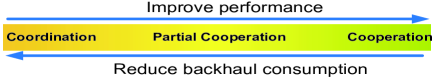
Figure 1: Illustration of the family of interference mitigation techniques.

$\bullet$ Delay-Aware Dynamic Partial Cooperative MIMO Control: The existing resource control designs for the partial cooperative MIMO schemes in [9] and [11] are adaptive to the CSI only. A common assumption in these existing works is that there are infinite backlogs at the transmitters and the applications are delay-insensitive. However, in practice, a lot of applications have bursty data arrivals and they are delay-sensitive. Therefore, it is very important to take into account the delay performance in designing partial cooperative MIMO schemes. To support delay-sensitive applications, the dynamic resource control should be jointly adaptive to the CSI and the QSI in the system to exploit the information regarding the transmission opportunity (provided by the CSI) and the data urgency (provided by the QSI). Striking an optimal balance between the transmission opportunity and the data urgency for delay-sensitive applications is very challenging, because it involves solving an infinite horizon stochastic optimization problem [13, Chap. 4]. The brute force solutions using stochastic optimization techniques [13, Chap. 4] lead to centralized delay-optimal control policies. These brute force solutions have exponential complexity with respect to (w.r.t.) the number of data streams and require the global QSI of all data streams. Therefore, it is highly desirable and challenging to obtain a low-complexity distributed delay-aware resource control design for practical multi-cell MIMO networks.

$\bullet$ Impact of Imperfect CSIT: The resource control designs for the partial cooperative MIMO schemes in [9] and [11] assume perfect CSIT. In practice, the CSIT may be imperfect due to the duplexing delay in TDD systems [14] or feedback latency and quantization in FDD systems [15]. With imperfect CSIT, there may be packet errors in each frame due to the uncertainty of the mutual information at the transmitters. Thus, it is important to take into account the CSIT errors in the resource optimization design. Yet, this requires explicit knowledge of the statistics of the CSIT errors and the bursty data arrivals. It is quite challenging to have a robust solution w.r.t. uncertainty in the modeling.

I-B Main Contributions

In this paper, we consider a general multi-BS multi-antenna MIMO network, the system model of which is presented in Section II. In Section III, we propose a novel Pco-MIMO PHY scheme, which allows flexible tradeoff between the MIMO cooperation level and the backhaul consumption. In Section IV, we formulate the delay-optimal transmit power and rate allocation (according to the imperfect CSIT and the QSI) under average power and backhaul consumption constraints as an infinite horizon average cost constrained partially observed Markov decision process (CPOMDP) [13, Chap. 4], [16], [17]. By exploiting the special structure in our problem, we derive an equivalent optimality equation to solve the CPOMDP in Section V. In Section VI, we propose a distributed online power and rate control solution using a distributed stochastic learning algorithm and a distributed online stochastic partial gradient algorithm. The proposed solution has very low complexity and requires only local observations of the system states at the BSs. Hence, it can be implemented distributively and is very robust against model variations. We also establish technical conditions for the convergence and asymptotic optimality of the proposed solution. We demonstrate the significant performance gain of the proposed scheme compared with various baseline schemes using numerical simulations in Section VII. Finally, conclusions are provided in Section VIII.

I-C Notation

$\mathbb{C}$ and $\mathbb{R}$ denote the sets of complex and real numbers, respectively. $\mathbb{E}[\cdot]$ and $\mathbf{1}(\cdot)$ denote expectation and the indicator function, respectively. $|\cdot|$ denotes the absolute value function for a scalar or the cardinality for a set. $(\cdot)^{T}$ and $(\cdot)^{\dagger}$ denote the transpose and Hermitian transpose, respectively. $\lfloor\cdot\rfloor$ denotes the floor function. $[x]^{+}=\max(x,0)$ and $[x]_{\bigwedge N_{Q}}=\min(x,N_{Q})$. $\text{diag}(a_{1},\cdots,a_{n})$ denotes a diagonal matrix with diagonal entries $a_{1},\cdots,a_{n}$. $\text{Null}(\mathbf{H})$ denotes the null space of matrix $\mathbf{H}$. $[\mathbf{H}]_{(l,m)}$ denotes the $(l,m)$-th element of $\mathbf{H}$.

II System Model

II-A System Topology

We consider the downlink transmission of a MIMO network with $K$ multi-antenna BSs delivering $K$ delay-sensitive data flows to $K$ multi-antenna MSs, where $K\geq 2$. Fig. 2 illustrates an example with $K=2$. Specifically, each BS is equipped with $M$ antennas, while each MS is equipped with $N$ antennas, where $\frac{M}{K}<N\leq M$ . Furthermore, we consider the e-NodeB architecture in LTE systems [18], where every two BSs are connected by a bi-directional backhaul link with limited capacity in each direction. Denote $\mathcal{K}\triangleq\{1,2,\cdots,K\}$. Each BS $k$ has one MS (indexed by $k$) in its cell and maintains a queue for the bursty data flow towards MS $k$, where $k\in\mathcal{K}$. BS $k$ is the master BS for serving MS $k$, while the other BSs $n\in\mathcal{K},n\neq k$ cooperatively serve MS $k$ according to the proposed Pco-MIMO scheme, which will be illustrated in Section III-A. The time dimension is partitioned into scheduling frames indexed by $t$ with frame duration $\tau$ (seconds).

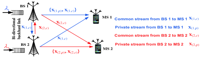
Figure 2: System Model for $K=2$. There are two multi-antenna BSs connected by a bi-directional backhaul link with limited backhaul capacity. The flows into BS 1 and BS 2 are targeted to MS 1 and MS 2, respectively. The data streams to each MS are split into common streams and private streams. The common streams are shared through the backhaul and jointly transmitted by the two BSs. The private streams are transmitted locally at each BS to its target MS.

II-B MIMO Channel and Imperfect CSIT Models

Let $\mathbf{s}_{n}\in\mathbb{C}^{M\times 1}$ be the complex signal vector transmitted by BS $n$ and $\mathbf{z}_{k}\in\mathbb{C}^{N\times 1}$ be the circularly symmetric Additive White Gaussian Noise (AWGN) vector at MS $k$, where $n,k\in\mathcal{K}$. We assume all noise terms are i.i.d. zero mean complex Gaussian with $\mathbb{E}[\mathbf{z}_{k}(\mathbf{z}_{k})^{H}]=\mathbf{I}_{N}$. The MIMO channel output $\mathbf{y}_{k}\in\mathbb{C}^{N\times 1}$ at MS $k\in\mathcal{K}$ is given by:

$$\mathbf{y}_{k}=\sum\nolimits_{n\in\mathcal{K}}\mathbf{H}_{kn}{\color[rgb]{0,0,0}\mathbf{s}_{n}}+\mathbf{z}_{k},$$ (1)

where $\mathbf{H}_{kn}\in\mathcal{H}^{N\times M}$ is the MIMO complex fading coefficient (CSI) from BS $n$ to MS $k$ and $\mathcal{H}\subset\mathbb{C}$ denotes the finite discrete CSI state space. Let $\mathbf{H}_{kn}(t)$ denote the CSI from BS $n$ to MS $k$ at frame $t$. We have the following assumption on the CSI.

Assumption 1 (CSI Model)

The $(i,l)$-th element $[\mathbf{H}_{kn}]_{(i,l)}(t)$ is constant within each frame and i.i.d. over scheduling frame $t$ following a general distribution over $\mathcal{H}$. $\{[\mathbf{H}_{kn}]_{(i,l)}(t)\}$ is independent w.r.t. $\{k,n,i,l\}$. Assume $\text{rank}(\mathbf{H}_{kn}(t))=\min(M,N)$ with probability 1. The BSs do not have knowledge of the CSI distribution $\Pr\{\mathbf{H}_{kn}\}$.  ∎

We assume that each MS has perfect knowledge of the CSI (perfect CSIR) but each BS only has imperfect knowledge of the CSI (imperfect CSIT). Thus, $\mathbf{H}_{kn}\in\mathcal{H}^{N\times M}$ also denotes the (accurate) MIMO complex fading coefficient from BS $n$ to MS $k$ estimated at MS $k$. Let $\hat{\mathbf{H}}_{kn}\in\hat{\mathcal{H}}^{N\times M}$ denote the imperfect MIMO complex fading coefficient from BS $n$ to MS $k$ estimated (with error) at BS $n$, where $\hat{\mathcal{H}}\subset\mathbb{C}$ denotes the finite discrete CSIT state space.

Assumption 2 (Imperfect CSIT Model)

The imperfect CSIT $\mathbf{\hat{H}}_{kn}$ is stochastically related to the actual CSI $\mathbf{H}_{kn}$ via the CSIT error kernel $\Pr\{\mathbf{\hat{H}}_{kn}|\mathbf{H}_{kn}\}$. Assume $\text{rank}(\hat{\mathbf{H}}_{kn})=\min(M,N)$ with probability 1. The BSs do not have knowledge of the CSIT error kernel.  ∎

The imperfect CSIT model in Assumption 2 is very general and covers most of the cases we encounter in practice, e.g., the imperfect CSIT due to duplexing delay in TDD systems [14] or feedback latency and quantization in FDD systems [15]. We denote $\mathbf{H}=\{\mathbf{H}_{kn}:k,n\in\mathcal{K}\}$ and $\hat{\mathbf{H}}=\{\hat{\mathbf{H}}_{kn}:k,n\in\mathcal{K}\}$ as the global CSI and the global CSIT, respectively.

II-C Bursty Source Model and Queue Dynamics

Let $\mathbf{A}(t)=\{A_{k}(t):k\in\mathcal{K}\}$ be the random new arrivals (number of bits) to the $K$ BSs at the end of frame $t$.

Assumption 3 (Bursty Source Model)

The arrival $A_{k}(t)$ is i.i.d. over scheduling frame $t$ and follows a general distribution. The average arrival rate is $\lambda_{k}=\mathbb{E}[A_{k}]$. Furthermore, the random arrival process $\{A_{k}{\color[rgb]{0,0,0}(t)}\}$ is independent w.r.t. $k$.   ∎

Let $\mathbf{Q}(t)=\{Q_{k}(t):k\in\mathcal{K}\}\in\boldsymbol{\mathcal{Q}}$ denote the global QSI at the beginning of frame $t$, where $\boldsymbol{\mathcal{Q}}$ is the state space for the global QSI. $N_{Q}$ denotes the buffer size (number of bits). The queue dynamics of MS $k\in\mathcal{K}$ is given by:

$$\begin{array}[]{lll}\color[rgb]{0,0,0}Q_{k}(t+1)=\Big{[}\big{[}Q_{k}(t)-U_{k}(t)\big{]}^{+}+A_{k}(t)\Big{]}_{\bigwedge N_{Q}},\end{array}$$ (2)

where $U_{k}(t)$ is the goodput (number of bits successfully received) at MS $k$ at the end of frame $t$. The expression of $U_{k}(t)$ will be given in (18) .

II-D Power Consumption Model

At frame $t$, the total power consumption $P_{k}(t)$ of BS $k\in\mathcal{K}$ is contributed by the constant circuit power of the RF chains (such as the mixers, synthesizers and digital-to-analog converters) $P_{cct}$ and the transmit power of the power amplifier (PA) $P_{k}^{tx}(t)$ as follows:

$$P_{k}(t)=P_{k}^{tx}(t)+P_{\text{cct}}\mathbf{1}(P_{k}^{tx}(t)>0).$$ (3)

$P_{\text{cct}}$ is constant irrespective of $P_{k}^{tx}(t)$. The expression of $P_{k}^{tx}(t)$ will be given in (19).

III Partial Cooperative MIMO and DoF Analysis

In this section, we first propose a novel Partial Cooperative MIMO (Pco-MIMO) PHY scheme. Then, we analyze the associated system DoF performance.

III-A Partial Cooperative MIMO Scheme

As illustrated in Fig. 2, the data streams to each MS $k\in\mathcal{K}$ are split into $d_{(k,c)}\in\mathbb{N}$ common streams and $d_{(k,p)}\in\mathbb{N}$ private streams, where $\mathbb{N}$ denotes the set of natural numbers. The common streams are shared through the backhaul and jointly transmitted by the $K$ BSs. As a result, some backhaul capacity is consumed. On the other hand, the private streams are transmitted locally at each BS and no backhaul consumption is incurred. We adopt zero-forcing (ZF) precoder and decorrelator designs at the BSs and MSs, respectively. To fully eliminate interference and recover $d_{(k,c)}$ common streams and $d_{(k,p)}$ private streams at each MS $k$ when the CSIT is perfect, we have some conditions on $d_{(k,c)}$ and $d_{(k,p)}$ for all $k\in\mathcal{K}$. First, to transmit common streams using MIMO cooperation at the $K$ BSs, we require $d_{(k,c)}\leq\min(KM,N)=N$. Next, $d_{K,M,N}\triangleq[M-(K-1)N]^{+}$ private streams to MS $k$ can be zero-forced at BS $k$ to eliminate interference at MS $n\in\mathcal{K},n\neq k$. Thus, we can choose $d_{(k,p)}$ satisfying $d_{K,M,N}\leq d_{(k,p)}\leq\min(M,N)=N$. (Note that this condition is valid as the assumption $\frac{M}{K}<N$ implies $d_{K,M,N}<N$.) Finally, for each MS $k$ to eliminate the residual interference from the remaining $d_{n,p}-d_{K,M,N}$ private streams to MS $n$ using ZF decorrelation and detect all the desired streams, we require $d_{(k,p)}+d_{(k,c)}+\sum_{n\in\mathcal{K},n\neq k}\left(d_{(n,p)}-d_{K,M,N}\right)\leq N$. Therefore, we have the following feasibility constraints on $\{d_{(k,c)},d_{(k,p)}:k\in\mathcal{K}\}$:

$$d_{(k,p)}\geq d_{K,M,N},\ d_{(k,c)}+\sum_{n\in\mathcal{K}}d_{(n,p)}\leq N+(K-1)d_{K,M,N},\ \forall k\in\mathcal{K}.$$ (4)

Note that (4) implies

$$d_{(k,c)}\leq N-d_{K,M,N},\ \forall k\in\mathcal{K}.$$ (5)

Let $x_{(k,c)}^{i}$ denote the $i$-th common stream transmitted from the $K$ BSs to MS $k$, where $i\in\{1,\cdots,d_{(k,c)}\}$. Let $x_{(k,p)}^{i}$ denote the $i$-th private stream transmitted from BS $k$ to MS $k$, where $i\in\{1,\cdots,d_{(k,p)}\}$. Furthermore, let $P_{(k,c)}^{i}$ and $P_{(k,p)}^{i}$ denote the transmit power for $x_{(k,c)}^{i}$ and $x_{(k,p)}^{i}$, respectively. Let $\mathbf{b}_{(k,c)}^{i}\in\mathbb{C}^{{\color[rgb]{0,0,0}K}M\times 1}$ denote the joint precoder for $x_{(k,c)}^{i}$ at the $K$ BSs, where $|\mathbf{b}_{(k,c)}^{i}|=1$. Let $\mathbf{b}_{(k,p)}^{i}\in\mathbb{C}^{M\times 1}$ denotes the precoder for $x_{(k,p)}^{i}$ at BS $k$, where $|\mathbf{b}_{(k,p)}^{i}|=1$. Let $\mathbf{s}_{k}\in\mathbb{C}^{M\times 1}$ be the complex signal vector transmitted by BS $k$. Then, the complex signal vector transmitted by the $K$ BSs is given by:

$$\begin{bmatrix}\mathbf{s}_{1}\\ \vdots\\ \mathbf{s}_{K}\end{bmatrix}=\sum_{k\in\mathcal{K}}\left(\mathbf{B}_{(k,c)}\Sigma_{(k,c)}\mathbf{x}_{(k,c)}\right)+\begin{bmatrix}\mathbf{B}_{(1,p)}\Sigma_{(1,p)}\mathbf{x}_{(1,p)}\\ \vdots\\ \mathbf{B}_{(K,p)}\Sigma_{(K,p)}\mathbf{x}_{(K,p)}\end{bmatrix},$$ (6)

$$\text{where }\mathbf{B}_{(k,c)}=[\mathbf{b}_{(k,c)}^{1},\cdots,\mathbf{b}_{(k,c)}^{d_{(k,c)}}]\in\mathbb{C}^{{\color[rgb]{0,0,0}K}M\times{d_{(k,c)}}},\quad\mathbf{B}_{(k,p)}=[\mathbf{b}_{(k,p)}^{1},\cdots,\mathbf{b}_{(k,p)}^{d_{(k,p)}}]\in\mathbb{C}^{M\times{d_{(k,p)}}},$$

$$\Sigma_{(k,c)}=\text{diag}(\sqrt{P_{(k,c)}^{1}},\cdots,\sqrt{P_{(k,c)}^{d_{(k,c)}}}),\quad\Sigma_{(k,p)}=\text{diag}(\sqrt{P_{(k,p)}^{1}},\cdots,\sqrt{P_{(k,p)}^{d_{(k,p)}}})$$

$$\mathbf{x}_{(k,c)}=[x_{(k,c)}^{1},\cdots,x_{(k,c)}^{d_{(k,c)}}]^{T},\quad\mathbf{x}_{(k,p)}=[x_{(k,p)}^{1},\cdots,x_{(k,p)}^{d_{(k,p)}}]^{T}.$$

Substituting (6) into (1), the received signal $\mathbf{y}_{k}\in\mathbb{C}^{N\times 1}$ at each MS $k\in\mathcal{K}$ is given by:

$$\begin{array}[]{lll}&\mathbf{y}_{k}=\underbrace{\mathbf{H}_{k}\mathbf{B}_{(k,c)}\Sigma_{(k,c)}\mathbf{x}_{(k,c)}+\mathbf{H}_{kk}\mathbf{B}_{(k,p)}\Sigma_{(k,p)}\mathbf{x}_{(k,p)}}_{\text{desired signals for MS $k$}}+\underbrace{{\color[rgb]{0,0,0}\sum_{n\in\mathcal{K},n\neq k}}\mathbf{H}_{k}\mathbf{B}_{(n,c)}\Sigma_{(n,c)}\mathbf{x}_{(n,c)}}_{\text{interference from common streams {\color[rgb]{0,0,0}to MS} $n$}}\\ &+\underbrace{{\color[rgb]{0,0,0}\sum_{n\in\mathcal{K},n\neq k}}\mathbf{H}_{kn}\mathbf{B}_{(n,p)}^{(1)}\Sigma_{(n,p)}^{(1)}\mathbf{x}_{(n,p)}^{(1)}}_{\text{interference from first ${\color[rgb]{0,0,0}d_{K,M,N}}$ private streams {\color[rgb]{0,0,0}to MS} $n$}}+\underbrace{{\color[rgb]{0,0,0}\sum_{n\in\mathcal{K},n\neq k}}\mathbf{H}_{kn}\mathbf{B}_{(n,p)}^{(2)}\Sigma_{(n,p)}^{(2)}\mathbf{x}_{(n,p)}^{(2)}}_{\text{interference from last $d_{(n,p)}-{\color[rgb]{0,0,0}d_{K,M,N}}$ private streams {\color[rgb]{0,0,0}to MS} $n$}}\\ &+\mathbf{z}_{k},\end{array}$$ (7)

where $\mathbf{H}_{k}=\left[\mathbf{H}_{k1},\cdots,\mathbf{H}_{kK}\right]\in\mathbb{C}^{N\times KM}$ and

$$\mathbf{B}_{(n,p)}^{(1)}=[\mathbf{b}_{(n,p)}^{1},\cdots,\mathbf{b}_{(n,p)}^{d_{K,M,N}}]\in\mathbb{C}^{M\times d_{K,M,N}},\ \mathbf{B}_{(n,p)}^{(2)}=[\mathbf{b}_{(n,p)}^{d_{K,M,N}+1},\cdots,\mathbf{b}_{(n,p)}^{d_{(n,p)}}]\in\mathbb{C}^{M\times\left(d_{(k,p)}-d_{K,M,N}\right)},$$

$$\Sigma_{(k,p)}^{(1)}=\text{diag}(\sqrt{P_{(k,p)}^{1}},\cdots,\sqrt{P_{(k,p)}^{d_{K,M,N}})},\ \Sigma_{(k,p)}^{(2)}=\text{diag}(\sqrt{P_{(k,p)}^{d_{K,M,N}+1}},\cdots,\sqrt{P_{(k,p)}^{d_{(k,p)}})},$$

$$\mathbf{x}_{(n,p)}^{(1)}=[x_{(n,p)}^{1},\cdots,x_{(n,p)}^{d_{K,M,N}}]^{T},\ \mathbf{x}_{(n,p)}^{(2)}=[x_{(n,p)}^{d_{K,M,N}+1},\cdots,x_{(n,p)}^{d_{(n,p)}}]^{T}.$$

Note that $\mathbf{B}_{(n,p)}=[\mathbf{B}_{(n,p)}^{(1)},\mathbf{B}_{(n,p)}^{(2)}]$, $\mathbf{\Sigma}_{(n,p)}=\left[\mathbf{\Sigma}_{(n,p)}^{(1)},0\atop 0,\mathbf{\Sigma}_{(n,p)}^{(2)}\right]$, and $\mathbf{x}_{(n,p)}=[(\mathbf{x}_{(n,p)}^{(1)})^{T},(\mathbf{x}_{(n,p)}^{(2)})^{T}]^{T}$. Let $\mathbf{u}_{(k,p)}^{i}\in\mathbb{C}^{N\times 1}$ and $\mathbf{u}_{(k,c)}^{i}\in\mathbb{C}^{N\times 1}$ be the decorrelators for $x_{(k,p)}^{i}$ and $x_{(k,c)}^{i}$, respectively. After decorrelation, the recovered signals $r_{(k,c)}^{i}$ and $r_{(k,p)}^{i}$ for $x_{(k,c)}^{i}$ and $x_{(k,p)}^{i}$ at MS $k$ are:

$$r_{(k,c)}^{i}=(\mathbf{u}_{(k,c)}^{i})^{{\dagger}}\mathbf{y}_{k},\quad r_{(k,p)}^{i}=(\mathbf{u}_{(k,p)}^{i})^{{\dagger}}\mathbf{y}_{k}.$$ (8)

In the following, we present the precoder and decorrelator designs for the Pco-MIMO under perfect CSIT, i.e., $\hat{\mathbf{H}}=\mathbf{H}$. Note that when the CSIT is imperfect, the precoders at the BSs are designed according to imperfect CSIT $\hat{\mathbf{H}}$ instead of $\mathbf{H}$. Thus, there will be residual interference from the common streams and the first $d_{K,M,N}$ private streams for other MSs even after the imperfect ZF precoding. The impact of the imperfect CSIT will be discussed in Section III-C.

III-A1 Precoder Design for Pco-MIMO

First, we design the precoder $\mathbf{B}_{(n,c)}$ at the $K$ BSs for the common streams $\mathbf{x}_{(n,c)}$, where $n\in\mathcal{K}$. To eliminate the interference term $\mathbf{H}_{k}\mathbf{B}_{(n,c)}\Sigma_{(n,c)}\mathbf{x}_{(n,c)}$ in (7) experienced by MS $k\neq n$, the joint ZF precoder $\mathbf{B}_{(n,c)}\in\mathbb{C}^{{\color[rgb]{0,0,0}K}M\times{d_{(n,c)}}}$ at the $K$ BSs is given by [19]:

$$\color[rgb]{0,0,0}\mathbf{B}_{(n,c)}=\widetilde{\mathbf{B}}_{{\color[rgb]{0,0,0}n}}\mathbf{F}_{(n,c)},$$ (9)

where the columns of $\widetilde{\mathbf{B}}_{n}\in\mathbb{C}^{{\color[rgb]{0,0,0}K}M\times({\color[rgb]{0,0,0}K}M-N)}$ form the orthonormal basis of

$$\text{Null}({\color[rgb]{0,0,0}\left[\mathbf{H}_{1}^{T},\cdots,\mathbf{H}_{n-1}^{T},\mathbf{H}_{n+1}^{T},\cdots,\mathbf{H}_{K}^{T}\right]^{T}}).$$

$\mathbf{F}_{(n,c)}=[\mathbf{\overline{b}}_{(n,c)}^{1},\cdots,\mathbf{\overline{b}}_{(n,c)}^{d_{(n,c)}}]\in\mathbb{C}^{({\color[rgb]{0,0,0}K}M-N)\times d_{({\color[rgb]{0,0,0}n},c)}}$ is designed by performing SVD on $\mathbf{H}_{n}\widetilde{\mathbf{B}}_{{\color[rgb]{0,0,0}n}}$ [20], i.e., $\mathbf{H}_{n}\widetilde{\mathbf{B}}_{{\color[rgb]{0,0,0}n}}=\mathbf{\overline{U}}_{(n,c)}\overline{\Sigma}_{(n,c)}[\mathbf{\overline{b}}_{(n,c)}^{1},\cdots,\mathbf{\overline{b}}_{(n,c)}^{{\color[rgb]{0,0,0}K}M-N}]^{{\dagger}}$, where the eigenvalues in $\overline{\Sigma}_{(n,c)}$ are sorted in decreasing order along the diagonal. Therefore, the common streams $\mathbf{x}_{(n,c)}$ are transmitted on the dominant eigenmodes for the desired MS $n$.

Next, we design the precoders $\mathbf{B}_{(n,p)}^{(1)}$ and $\mathbf{B}_{(n,p)}^{(2)}$ at BS $n$ for the first ${\color[rgb]{0,0,0}d_{K,M,N}}$ private streams $\mathbf{x}_{(n,p)}^{(1)}$ and the last $d_{(n,p)}-{\color[rgb]{0,0,0}d_{K,M,N}}$ private streams $\mathbf{x}_{(n,p)}^{(2)}$, respectively. To eliminate the interference term $\mathbf{H}_{kn}\mathbf{B}_{(n,p)}^{(1)}\Sigma_{(n,p)}^{(1)}\mathbf{x}_{(n,p)}^{(1)}$ in (7) experienced by MS $k$, the ZF precoder $\mathbf{B}_{(n,p)}^{(1)}\in\mathbb{C}^{M\times{\color[rgb]{0,0,0}d_{K,M,N}}}$ at BS $n$ is given by:

$$\mathbf{B}_{(n,p)}^{(1)}=\widetilde{\mathbf{B}}_{kn}\mathbf{F}_{(n,{\color[rgb]{0,0,0}p})},$$ (10)

where the columns of $\widetilde{\mathbf{B}}_{kn}\in\mathbb{C}^{M\times{\color[rgb]{0,0,0}d_{K,M,N}}}$ form the orthonormal basis of $\text{Null}(\mathbf{H}_{kn})$ and $\mathbf{F}_{(n,{\color[rgb]{0,0,0}p})}\in\mathbb{C}^{{\color[rgb]{0,0,0}d_{K,M,N}}\times{\color[rgb]{0,0,0}d_{K,M,N}}}$ is designed by performing SVD on $\mathbf{H}_{nn}\widetilde{\mathbf{B}}_{kn}$, i.e., $\mathbf{H}_{nn}\widetilde{\mathbf{B}}_{kn}=\mathbf{\overline{U}}_{(n,{\color[rgb]{0,0,0}p})}\overline{\Sigma}_{(n,z)}(\mathbf{F}_{(n,{\color[rgb]{0,0,0}p})})^{{\dagger}}.$ The eigenvalues in $\overline{\Sigma}_{(n,{\color[rgb]{0,0,0}p})}$ are sorted in decreasing order along the diagonal. The precoder $\mathbf{B}_{(n,p)}^{(2)}\in\mathbb{C}^{M\times\left(d_{(n,p)}-{\color[rgb]{0,0,0}d_{K,M,N}}\right)}$ at BS $n$ is chosen to maximize the SNR of for the remaining $d_{(n,p)}-{\color[rgb]{0,0,0}d_{K,M,N}}$ private streams $\mathbf{x}_{(n,p)}^{(2)}$ of the MS $n$, i.e.,

$$\mathbf{B}_{(n,p)}^{(2)}=[\mathbf{\overline{b}}_{nn}^{1},\cdots,\mathbf{\overline{b}}_{nn}^{d_{(n,p)}-{\color[rgb]{0,0,0}d_{K,M,N}}}]$$ (11)

is obtained by performing SVD on $\mathbf{H}_{nn}$, i.e., $\mathbf{H}_{nn}=\mathbf{\widetilde{U}}_{nn}\widetilde{\Sigma}_{nn}[\mathbf{\overline{b}}_{nn}^{1},\cdots,\mathbf{\overline{b}}_{nn}^{M}]^{{\dagger}}.$ The eigenvalues in $\widetilde{\Sigma}_{nn}$ are sorted in decreasing order along the diagonal.

III-A2 Decorrelator Design for Pco-MIMO

First, we design the decorrelator $\mathbf{u}_{(k,p)}^{i}$ at MS $k$ for the $i$-th desired common stream $x_{(k,c)}^{i}$. To eliminate the residual interference from the remaining $d_{n,p}-{\color[rgb]{0,0,0}d_{K,M,N}}$ private streams to MS $n\in\mathcal{K},n\neq k$ and detect $x_{(k,c)}^{i}$, the decorrelator $\mathbf{u}_{(k,c)}^{i}\in\mathbb{C}^{N\times 1}$ at MS $k$ is given by:

$$\color[rgb]{0,0,0}\mathbf{u}_{(k,c)}^{i}=\mathbf{\widetilde{U}}_{(k,c)}(\mathbf{\widetilde{U}}_{(k,c)})^{{\dagger}}\mathbf{H}_{kk}\mathbf{b}_{(k,c)}^{i}/\psi,$$ (12)

where the columns of $\mathbf{\widetilde{U}}_{(k,c)}\in\mathbb{C}^{N\times(M-d_{(k,c)}-{\color[rgb]{0,0,0}\sum_{n\in\mathcal{K}}}d_{(n,p)}+1)}$ form the orthonormal basis of $\text{Null}(\mathbf{\widetilde{H}}_{(k,c)})$ and $\mathbf{\widetilde{H}}_{(k,c)}=\left[\mathbf{H}_{k}\mathbf{B}_{(k,c),i}^{(1)},\mathbf{H}_{kk}\mathbf{B}_{(k,p)}^{(1)},\mathbf{H}_{k1}\mathbf{B}_{(1,p)}^{(2)},\cdots,\mathbf{H}_{kK}\mathbf{B}_{(K,p)}^{(2)}\right].$ $\mathbf{B}_{(k,c),i}^{(1)}$ is $\mathbf{B}_{(k,c)}^{(1)}$ without the $i$-th column, i.e., $\mathbf{B}_{(k,c),i}^{(1)}=\left[\mathbf{b}_{(k,c)}^{1},\cdots,\mathbf{b}_{(k,c)}^{i-1},\mathbf{b}_{(k,c)}^{i+1},\cdots,\mathbf{b}_{(k,c)}^{d_{(k,c)}}\right]$. Here, $\psi=||\mathbf{\widetilde{U}}_{(k,c)}(\mathbf{\widetilde{U}}_{(k,c)})^{{\dagger}}\mathbf{H}_{kk}\mathbf{b}_{(k,c)}^{i}||$ is to normalize $\mathbf{u}_{(k,c)}^{i}$, i.e., $||\mathbf{u}_{(k,c)}^{i}||=1$. By using the decorrelator in (12), the interference is nulled due to the fact that $(\mathbf{\widetilde{U}}_{(k,c)})^{{\dagger}}\mathbf{\widetilde{H}}_{(k,c)}=0$. The equivalent channel for $x_{(k,c)}^{i}$ is $(\mathbf{u}_{(k,c)}^{i})^{{\dagger}}\mathbf{H}_{kk}\mathbf{b}_{(k,c)}^{i}\sqrt{P_{(k,c)}^{i}}=\frac{1}{\psi}||(\mathbf{\widetilde{U}}_{(k,c)})^{{\dagger}}\mathbf{H}_{kk}\mathbf{b}_{(k,c)}^{i}||^{2}\sqrt{P_{(k,c)}^{i}}.$ The decorrelator $\mathbf{u}_{(k,p)}^{i}\in\mathbb{C}^{N\times 1}$ at MS $k$ can be designed in a similar way to $\mathbf{u}_{(k,c)}^{i}$.

Remark 1 (Flexible Adjustment of Cooperation Level in Pco-MIMO)

The Pco-MIMO design is flexible to adjust the cooperation level between the coordination and cooperation modes. It also incorporates the full coordinative MIMO (by choosing $d_{(k,c)}=0$ for all $k\in\mathcal{K}$), the Uco-MIMO for $K=2$ (by choosing $d_{(k,c)}=0$ and $d_{(n,c)}>0$, where $k,n\in\{1,2\},n\neq k$) and the full cooperative MIMO (by choosing $d_{(k,p)}=0$ for all $k\in\mathcal{K}$) as special cases.   ∎

III-B DoF Performance under Perfect CSIT

We derive the system DoF of the Pco-MIMO scheme under the perfect CSIT.

Theorem 1 (DoF Performance of Pco-MIMO)

Suppose the backhaul consumption satisfies $R_{(k,c)}=d_{(k,c)}\log_{2}(\text{SNR})$ for all $k\in\mathcal{K}$. The system DoF under the Pco-MIMO scheme $\text{DoF}(\text{Pco-MIMO})=\sum_{k\in\mathcal{K}}(d_{(k,p)}+d_{(k,c)})$ satisfies

$$\text{DoF}(\text{Pco-MIMO})\leq\text{DoF}_{\max}(\text{Pco-MIMO})\triangleq N+(K-1)d_{K,M,N}+\min_{k\in\mathcal{K}}\sum_{n\in\mathcal{K},n\neq k}d_{(n,c)},$$ (13)

where the maximum system DoF $\text{DoF}_{\max}(\text{Pco-MIMO})$ can be achieved when

$$\ d_{(k,c)}+\sum_{n\in\mathcal{K}}d_{(n,p)}=N+(K-1)d_{K,M,N},\quad\forall k\in\arg\min_{k\in\mathcal{K}}\sum_{n\in\mathcal{K},n\neq k}d_{(n,c)}.$$ (14)

Furthermore, $\text{DoF}_{\max}(\text{Pco-MIMO})\leq KN$, where the equality holds when

$$d_{(n,c)}=N-d_{K,M,N},\quad\forall n\in\mathcal{K},n\neq k,k\in\arg\min_{k\in\mathcal{K}}\sum_{n\in\mathcal{K},n\neq k}d_{(n,c)}.$$ (15)

∎

Proof:

Please refer to Appendix A. ∎

From Theorem 1, we can see that the proposed Pco-MIMO scheme allows a flexible tradeoff between the achievable DoF and the backhaul consumption.

Scheme	Coordinative MIMO	Uco-MIMO	Pco-MIMO	Cooperative MIMO
DoF ($K=2$)	$M$	$M$	$\{M,\cdots,2N\}$	$2N$
DoF ($K>2$)	$N+(K-1)d_{K,M,N}$	not applicable	$\{N+(K-1)d_{K,M,N},\cdots,KN\}$	$KN$

TABLE I: Illustration of the system DoFs of different schemes at $d_{(k,c)}=d$ for all $k\in\mathcal{K}$.

Remark 2 (Comparisions of System DoFs)

Table I compares the system DoFs of different schemes. (Note that $d_{K,M,N}=M-N$ when $K=2$.) By choosing $d_{(k,c)}=d\leq N-d_{K,M,N}$ for all $k\in\mathcal{K}$, the proposed Pco-MIMO scheme can achieve $\text{DoF}(\text{Pco-MIMO})=N+(K-1)d_{K,M,N}+(K-1)d$, i.e., an increase of $(K-1)d$ compared with the coordinative MIMO or the uni-directional cooperative MIMO (Uco-MIMO) [21, 10] (applicable for $K=2$ only). This increase is achieved at the cost of the backhaul consumption of $(K-1)d\log_{2}(\text{SNR})$ (for each BS). By choosing $d_{(k,c)}=d=N-d_{K,M,N}$ for all $k\in\mathcal{K}$, the proposed Pco-MIMO scheme can achieve $\text{DoF}(\text{Pco-MIMO})=KN$, which is the same as the full cooperative MIMO, but save backhaul consumption by $(K-1)(N-d)\log_{2}(\text{SNR})=(K-1)d_{K,M,N}\log_{2}(\text{SNR})\geq 0$ (for each BS) compared with the full cooperative MIMO.  ∎

III-C Mutual Information, System Goodput under Imperfect CSIT

When the CSIT is imperfect, there will be residual interference at each MS due to imperfect ZF precoding. Given the decorrelator $\mathbf{u}_{(k,c)}^{i}$ of the $i$-th common stream, the recovered signal of $x_{(k,c)}^{i}$ in (8) at MS $k$ is given by:

$$\begin{array}[]{lll}{\color[rgb]{0,0,0}r_{(k,c)}^{i}}=(\mathbf{u}_{(k,c)}^{i})^{{\dagger}}\mathbf{y}_{k}=\underbrace{(\mathbf{u}_{(k,c)}^{i})^{{\dagger}}\mathbf{H}_{kk}\mathbf{b}_{(k,c)}^{i}\sqrt{P_{(k,c)}^{i}}x_{(k,c)}^{i}}_{\text{desired signal for MS $k$}}+\underbrace{(\mathbf{u}_{(k,c)}^{i})^{{\dagger}}\mathbf{I}_{k}}_{\text{residual interference at MS $k$}}+(\mathbf{u}_{(k,c)}^{i})^{{\dagger}}\mathbf{z}_{k},\end{array}$$

where $\mathbf{I}_{k}={\color[rgb]{0,0,0}\sum_{n\in\mathcal{K},n\neq k}}\left(\mathbf{H}_{kn}\mathbf{B}_{(n,p)}^{(1)}\Sigma_{(n,p)}^{(1)}\mathbf{x}_{(n,p)}^{(1)}+\mathbf{H}_{k}\mathbf{B}_{(n,c)}\Sigma_{(n,c)}\mathbf{x}_{(n,c)}\right)$. Assuming Gaussian inputs for the system and treating interference as noise, the mutual information (bit/s/Hz) of the $i$-th common stream at MS $k$ is given by:

$$C_{(k,c)}^{i}=\log_{2}\left(1+\sigma_{(k,c)}^{i}P_{(k,c)}^{i}/(1+I_{(k,c)}^{i})\right),\forall i=1,\cdots,d_{(k,c)},$$ (16)

where $\sigma_{(1,c)}^{i}=|(\mathbf{u}_{(k,c)}^{i})^{\dagger}\mathbf{H}_{kk}\mathbf{b}_{(k,c)}^{i}|^{2}$ and

$$I_{(k,c)}^{i}={\color[rgb]{0,0,0}\sum_{n\in\mathcal{K},n\neq k}}\left(\sum_{i=1}^{{\color[rgb]{0,0,0}d_{K,M,N}}}P_{(n,p)}^{i}|(\mathbf{u}_{(k,c)}^{i})^{{\dagger}}\mathbf{H}_{kn}\mathbf{b}_{(n,p)}^{i}|^{2}+\sum_{i=1}^{d_{(n,c)}}P_{(n,c)}^{i}\cdot|(\mathbf{u}_{(k,c)}^{i})^{{\dagger}}\mathbf{H}_{k}\mathbf{b}_{(n,c)}^{i}|^{2}\right).$$

Similarly, the mutual information (bit/s/Hz) of the $i$-th private stream at MS $k$ is given by:

$$C_{(k,p)}^{i}=\log_{2}\left(1+\sigma_{(k,p)}^{i}P_{(k,p)}^{i}/(1+I_{(k,p)}^{i})\right),\forall i=1,\cdots,d_{(k,p)},$$ (17)

where $\sigma_{(1,p)}^{i}=|(\mathbf{u}_{(k,p)}^{i})^{\dagger}\mathbf{H}_{kk}\mathbf{b}_{(k,p)}^{i}|^{2}$ and $I_{(k,p)}^{i}$ is calculated in a similar way to $I_{(k,c)}^{i}$.

Due to the imperfect CSIT, the mutual information $C_{(k,c)}^{i}$ and $C_{(k,p)}^{i}$ at a frame are not completely known to the BSs. Thus, there will be packet errors when the transmit data rate exceeds the mutual information. Let $R_{(k,c)}$ and $R_{(k,p)}$ be the scheduled data rate of the common streams and the private streams of BS $k$, respectively. (Note that $R_{(k,c)}$ also indicates the backhaul consumption for sharing common streams from BS $k$.) The goodput $U_{k}$ at MS $k$ (number of bits successfully received) in one frame is given by:

$$\color[rgb]{0,0,0}U_{k}=\tau R_{(k,c)}\mathbf{1}\big{(}R_{(k,c)}\leq C_{(k,c)}\big{)}+\tau R_{(k,p)}\mathbf{1}\big{(}R_{(k,p)}\leq C_{k,p}\big{)},$$ (18)

where $C_{(k,c)}=\sum_{i=1}^{d_{(k,c)}}C_{(k,c)}^{i}$, $C_{k,p}=\sum_{i=1}^{d_{(k,p)}}C_{(k,p)}^{i}$ and $\mathbf{1}(\cdot)$ denotes the indicator function.

The total transmit power of BS $k$ to support the $d_{(k,p)}$ private streams, the $d_{(k,c)}$ common streams to MS $k$ and the $d_{(n,c)}$ common streams to MS $n\in\mathcal{K},n\neq k$ is given by:

$$\begin{array}[]{l}P_{k}^{tx}=\sum\nolimits_{i=1}^{d_{(k,p)}}P_{(k,p)}^{i}+\sum_{n\in\mathcal{K}}P_{(n,c),k},\end{array}$$ (19)

where $P_{(n,c),k}=\sum\nolimits_{i=1}^{d_{(n,c)}}P_{(n,c)}^{i}\alpha_{(n,k)}^{i}$ denotes the transmit power at BS $k$ for the common streams to MS $n$ and $\alpha_{(n,k)}^{i}=\sum_{m=1}^{M}\big{|}[{\color[rgb]{0,0,0}\mathbf{B}_{(n,c)}}]_{((k-1)M+m,i)}\big{|}^{2}$ denotes the portion of power $P_{(n,c)}^{i}$ for common stream $x_{(n,c)}^{i}$ contributed by BS $k$. Note that each common stream is precoded at the $K$ BSs, and hence, we have $\sum_{k\in\mathcal{K}}\alpha_{(n,k)}^{i}=1$ for all $i=1,\cdots,d_{(n,c)}$, $n\in\mathcal{K}$.

IV Delay-Optimal Cross Layer Resource Optimization

In this section, we formally define the control policy and formulate the delay-optimal control problem under average power and backhaul constraints.

IV-A Control Policy and Resource Constraints

Denote $\boldsymbol{\chi}=\{\mathbf{H},\mathbf{Q}\}$ as the global system state and $\hat{\boldsymbol{\chi}}=\{\mathbf{\hat{H}},\mathbf{Q}\}$ as the observed global system state. The complete system state is $\{\boldsymbol{\chi},\hat{\boldsymbol{\chi}}\}$. Based on the Pco-MIMO scheme, at the beginning of each frame, determine the transmit power and rate allocation based on the global observed system state $\hat{\boldsymbol{\chi}}$ according to the following stationary control policy.

Definition 1 (Stationary Power and Rate Control Policy)

A stationary power and rate control policy $\Omega=\{\Omega_{P},\Omega_{R}\}$ is a mapping from the observed state $\hat{\boldsymbol{\chi}}$ to the power and rate allocation actions $\Omega(\hat{\boldsymbol{\chi}})=\{\Omega_{P}(\hat{\boldsymbol{\chi}}),\Omega_{R}(\hat{\boldsymbol{\chi}})\}$, where $\Omega_{P}(\hat{\boldsymbol{\chi}})=\mathbf{P}=\{\mathbf{P}_{(k,p)},\mathbf{P}_{(k,c)}:k\in\mathcal{K}\}$ and $\Omega_{R}(\hat{\boldsymbol{\chi}})=\mathbf{R}={\color[rgb]{0,0,0}\{\mathbf{R}_{k}:k\in\mathcal{K}\}}$. $\mathbf{P}_{(k,p)}=\{P_{(k,p)}^{i}\in\mathbb{R}^{+}:i=1,\cdots,d_{k,p}\}$, $\mathbf{P}_{(k,c)}=\{P_{(k,c)}^{i}\in\mathbb{R}^{+}:i=1,\cdots,d_{k,c}\}$, and $\mathbf{R}_{k}=\{R_{(k,p)},R_{(k,c)}\in\mathbb{R}^{+}\}$. Assume $\Omega$ is unichain.  ∎

The power allocation policy $\Omega_{P}$ satisfies the per-BS average power consumption constraint:

$$\overline{P}_{k}(\Omega)=\lim\sup_{T\rightarrow\infty}\frac{1}{T}\sum_{t=1}^{T}\mathbb{E}^{\Omega}[P_{k}(t)]\leq P_{k}^{0},\quad\forall k\in\mathcal{K},$$ (20)

where $\mathbb{E}^{\Omega}$ indicates that the expectation is taken w.r.t. the measure induced by the policy $\Omega$, $P_{k}(t)$ is the total power consumption of BS $k$ at frame $t$ given in (3), and $P_{k}^{0}$ denotes the maximum average power consumption. On the other hand, the rate allocation policy $\Omega_{R}$ satisfies the average backhaul consumption constraint:

$$\overline{R}_{(k,c)}(\Omega)=\lim\sup_{T\rightarrow\infty}\frac{1}{T}\sum\nolimits_{t=1}^{T}\mathbb{E}^{\Omega}[R_{(k,c)}(t)]\leq R_{(k,c)}^{0},\quad\forall k\in\mathcal{K},$$ (21)

where $R_{(k,c)}(t)$ is the scheduled data rate for the common streams $\mathbf{x}_{(k,c)}$ at frame $t$ and $R_{(k,c)}^{0}$ denotes the maximum average backhaul consumption.

IV-B Problem Formulation

For a given stationary control policy $\Omega$, the induced random process $\left\{\boldsymbol{\chi}(t),\hat{\boldsymbol{\chi}}(t)\right\}$ is a controlled Markov chain with the transition probability given by:

$$\Pr\{\boldsymbol{\chi}(t+1),\hat{\boldsymbol{\chi}}(t+1)|\boldsymbol{\chi}(t),\hat{\boldsymbol{\chi}}(t),\Omega(\hat{\boldsymbol{\chi}}(t))\}$$

$$= \Pr\{\mathbf{H}(t+1)\}\Pr\{\hat{\mathbf{H}}(t+1)|\mathbf{H}(t+1)\}\Pr\{\mathbf{Q}(t+1)|\boldsymbol{\chi}(t),\Omega(\hat{\boldsymbol{\chi}}(t))\},$$ (22)

where the queue transition probability is given by

$$\Pr\{\mathbf{Q}(t+1)|\boldsymbol{\chi}(t),\Omega(\hat{\boldsymbol{\chi}}(t))\}=\prod_{k\in\mathcal{K}}\Pr\left\{A_{k}(t)\in\mathbb{R}^{+}:A_{k}(t)\text{ satisfies }\eqref{eq:Q_org}\right\}$$ (23)

Note that, the stochastic dynamics of the $K$ queues are coupled together via $\Omega$.

Given a stationary control policy $\Omega$, the average delay cost of MS $k$ is given by:

$$\overline{T}_{k}(\Omega)=\lim\sup_{T\rightarrow\infty}\frac{1}{T}\sum\nolimits_{t=1}^{T}\mathbb{E}^{\Omega}\left[f(Q_{k}(t))\right],\quad\forall k\in\mathcal{K},$$ (24)

where $f(Q_{k})$ is a monotonic increasing cost function of $Q_{k}$. For example, when $f(Q_{k})=Q_{k}/\lambda_{k}$, by Little's Law [22], $\overline{T}_{k}(\Omega)$ is the average delay of user $k$. When $f(Q_{k})=\mathbf{1}(Q_{k}\geq Q_{k}^{0})$, $\overline{T}_{k}(\Omega)$ is the probability that $Q_{k}$ exceeds $Q_{k}^{0}$ for some reference $Q_{k}^{0}\in\{0,\cdots,N_{Q}\}$.

For some positive constants $\boldsymbol{\beta}=\{\beta_{k}:k\in\mathcal{K}\}$, define the average weighted sum delay cost under a stationary control policy $\Omega$ as:

$$\overline{T}_{\beta}^{\Omega}\triangleq\sum_{k\in\mathcal{K}}\beta_{k}\overline{T}_{k}(\Omega)=\lim\sup_{T\rightarrow\infty}\frac{1}{T}\sum\nolimits_{t=1}^{T}\mathbb{E}^{\Omega}\left[\sum_{k\in\mathcal{K}}\beta_{k}f(Q_{k}{\color[rgb]{0,0,0}(t)})\right]{\color[rgb]{0,0,0}.}$$

The delay-optimal control problem is formulated as follows:

Problem 1 (Delay-optimal Control Problem for Pco-MIMO)

$$\begin{array}[]{l}\min_{\Omega}\quad\overline{T}_{\beta}^{\Omega}\\ s.t.\quad\text{the average power and backhaul constraints in \eqref{eq:pwr_con} and \eqref{eq:bkh_con} {\color[rgb]{0,0,0}for all $k\in\mathcal{K}$}}{\color[rgb]{0,0,0}.}\end{array}$$

Note that under the time average expected constraints in (20) and (21), the probability, that the instantaneous power and backhaul consumption goes to infinity, goes to zero. Furthermore, additional peak power or backhaul consumption constraints can be accommodated in Problem 1.

Remark 3 (Interpretation of Problem 1)

Problem 1 is an infinite horizon constrained average cost per stage problem [13, Chap.4] or constrained Markov decision process (MDP)[16]. Specifically, since the control policy is defined on the observed system state $\hat{\boldsymbol{\chi}}$ instead of the complete system state $\{\boldsymbol{\chi},\hat{\boldsymbol{\chi}}\}$, Problem 1 belongs to constrained partially observed MDP (CPOMDP), which is well-known to be a very difficult problem [17].  ∎

V General Solution to the Delay Optimal Problem

In this section, by exploiting the special structure in our problem, we derive an equivalent Bellman equation to simplify the CPOMDP problem.

We consider the dual problem of the CPOMDP in Problem 1. For any nonnegative Lagrange multipliers (LMs) $\boldsymbol{\gamma}=\{\gamma_{(k,P)},\gamma_{(k,C)}\in\mathbb{R}^{+}:k\in\mathcal{K}\}$, define the Lagrangian as $L_{\beta}(\Omega,\boldsymbol{\gamma})=\lim\sup_{T\rightarrow\infty}\frac{1}{T}\sum\nolimits_{t=1}^{T}\mathbb{E}^{\Omega}\left[g\left(\boldsymbol{\gamma},\boldsymbol{\chi}(t),\Omega(\hat{\boldsymbol{\chi}}(t))\right)\right]$, where $g(\boldsymbol{\gamma},\boldsymbol{\chi},\Omega(\hat{\boldsymbol{\chi}}))=\sum_{k\in\mathcal{K}}\big{(}\beta_{k}f(Q_{k})+\gamma_{(k,P)}$ $(P_{k}-{\color[rgb]{0,0,0}P_{k}^{0}})+\gamma_{(k,C)}(R_{(k,c)}-{\color[rgb]{0,0,0}R_{(k,c)}^{0}})\big{)}.$ The associated dual problem of Problem 1 is given by

$$\max_{\boldsymbol{\gamma}\succeq 0}G(\boldsymbol{\gamma}),$$ (25)

where the Lagrange dual function (unconstrained POMDP) is given by:

$$G(\boldsymbol{\gamma})=\min_{\Omega}L_{\beta}(\Omega,\boldsymbol{\gamma}).$$ (26)

We discuss the solution to the dual problem in (25) and the duality gap below.

While POMDP is a difficult problem in general, we utilize the i.i.d. assumption of the CSI to substantially simplify the unconstrained POMDP in (26). The optimal control policy $\Omega^{*}$, can be obtained by solving an equivalent optimality equation, which is summarized below.

Theorem 2 (Equivalent Bellman Equation)

   

(a) For any given LMs $\boldsymbol{\gamma}$, the optimal control policy $\Omega^{*}=(\Omega_{P}^{*},\Omega_{R}^{*})$ for the unconstrained POMDP in (26) can be obtained by solving the following equivalent Bellman equation w.r.t. $\theta$ and $\{V(\widetilde{\mathbf{Q}})\}$:

$$V(\widetilde{\mathbf{Q}})+\theta= \mathbb{E}\left[\min_{\mathbf{P},\mathbf{R}}\mathbb{E}\left[g(\boldsymbol{\gamma},\boldsymbol{\chi},\mathbf{P},\mathbf{R})+\sum\nolimits_{\widetilde{\mathbf{Q}}^{\prime}}\Pr\{\widetilde{\mathbf{Q}}^{\prime}|\boldsymbol{\chi},\mathbf{P},\mathbf{R}\}V(\widetilde{\mathbf{Q}}^{\prime})\bigg{|}\hat{\boldsymbol{\chi}}\right]\Bigg{|}\widetilde{\mathbf{Q}}\right],\ \forall\widetilde{\mathbf{Q}}\in\boldsymbol{\mathcal{Q}},$$ (27)

where $\theta=G(\boldsymbol{\gamma})$ is the optimal average cost per stage and $V(\cdot)$ is the post-decision state potential function. $\widetilde{\mathbf{Q}}$ is the post-decision state, $\mathbf{Q}=[\widetilde{\mathbf{Q}}+\mathbf{A}]_{\bigwedge N_{Q}}$ is the pre-decision state, and $\widetilde{\mathbf{Q}}^{\prime}=(\mathbf{Q}-\mathbf{U})^{+}$ is the next post-decision state transited from $\mathbf{Q}$[25, Chap. 3], where $\mathbf{U}=\{U_{k}:k\in\mathcal{K}\}$.

(b) If $\Omega^{*}(\hat{\boldsymbol{\chi}})=\arg\min_{\mathbf{P},\mathbf{R}}\mathbb{E}\left[g(\boldsymbol{\gamma},\boldsymbol{\chi},\mathbf{P},\mathbf{R})+\sum\nolimits_{\widetilde{\mathbf{Q}}^{\prime}}\Pr\{\widetilde{\mathbf{Q}}^{\prime}|\boldsymbol{\chi},\mathbf{P},\mathbf{R}\}V(\widetilde{\mathbf{Q}}^{\prime})\bigg{|}\hat{\boldsymbol{\chi}}\right]$ is unique for all $\hat{\boldsymbol{\chi}}$, then the deterministic policy $\Omega^{*}$ is the optimal policy for the unconstrained POMDP in (26).  ∎

Proof:

Please refer to Appendix B. ∎

Note that the optimization problem in Problem 1 is not convex w.r.t. the control policy $\Omega$. The following lemma establishes the zero duality gap between the primal and dual problems.

Lemma 1 (Zero Duality Gap)

If the condition of Theorem 2 (b) holds, the duality gap between the primal problem in Problem 1 and the dual problem in (25) is zero, i.e.,

$$\min_{\Omega}\max_{\boldsymbol{\gamma}\succeq 0}L_{\beta}(\Omega,\boldsymbol{\gamma})=\max_{\boldsymbol{\gamma}\succeq 0}\min_{\Omega}L_{\beta}(\Omega,\boldsymbol{\gamma}).$$ (28)

Proof:

Please refer to Appendix C. ∎

Therefore, by solving the dual problem in (25), we can obtain the primal optimal $\Omega^{*}$. In other words, the derived policy of the equivalent Bellman equation in (27) for dual optimal LMs $\boldsymbol{\gamma}^{*}$ solves the CPOMDP (primal problem) in Problem 1.

Remark 4 (Discussions on Optimal Solution)

The brute-force solution using Theorem 2 and Lemma 1 requires solving a large system of nonlinear fixed point equations in (27). The obtained optimal solution has exponential complexity w.r.t. the number of MSs and requires centralized implementation and knowledge of system statistics. In the following section, we study a low-complexity distributed solution based on the optimal solution.

VI Low Complexity Distributed Solution

In this section, we propose a low-complexity distributed solution using a distributed online learning algorithm to estimate the per-flow potential functions and LMs and a distributed online stochastic partial gradient algorithm to obtain the power and rate control policy.

VI-A Linear Approximation of System Potential Functions

To reduce computational complexity and facilitate distributed implementation, we first approximate the system post-decision state potential functions $\{V(\widetilde{\mathbf{Q}})\}$ defined in (27) by the sum of the per-flow post-decision state potential functions $\{V_{k}(\widetilde{Q}_{k})\}$ for all $k\in\mathcal{K}$ below:

$$V(\widetilde{\mathbf{Q}})\approx\sum_{k\in\mathcal{K}}V_{k}(\widetilde{Q}_{k}),\quad\forall\widetilde{\mathbf{Q}}\in\boldsymbol{\mathcal{Q}},$$ (29)

where $\{V_{k}(\widetilde{Q}_{k})\}$ is defined as the fixed point of the following per-flow fixed point equation:

$$V_{k}(\widetilde{Q}_{k})+V_{k}(\widetilde{Q}_{k}^{0})$$ (30)

$$= \mathbb{E}\left[\min_{\mathbf{P}_{k},\mathbf{R}_{k}}\left[g_{k}(\boldsymbol{\gamma}_{k},\hat{\boldsymbol{\chi}}_{k},\mathbf{P}_{k},\mathbf{R}_{k})+\sum_{\widetilde{Q}_{k}^{\prime}}\Pr\{\widetilde{Q}_{k}^{\prime}|\hat{\boldsymbol{\chi}}_{k},\mathbf{P}_{k},\mathbf{R}_{k}\}V_{k}(\widetilde{Q}_{k}^{\prime})\right]\Bigg{|}\widetilde{Q}_{k}\right].$$

$g_{k}(\boldsymbol{\gamma}_{k},\hat{\boldsymbol{\chi}}_{k},\mathbf{P}_{k},\mathbf{R}_{k})=\beta_{k}f(Q_{k})+\gamma_{(k,P)}\left(\sum\nolimits_{i=1}^{d_{(k,p)}}P_{(k,p)}^{i}+P_{\text{cct}}\mathbf{1}(\sum\nolimits_{i=1}^{d_{(k,p)}}P_{(k,p)}^{i}>0)-P_{k}^{0}\right)+\sum_{n\in\mathcal{K},n\neq k}\gamma_{(n,P)}P_{(k,c),n}+\gamma_{(k,C)}(R_{(k,c)}-R_{(k,c)}^{0})$, $\boldsymbol{\gamma}_{k}=\{\gamma_{(k,C)},\gamma_{(n,P)}:n\in\mathcal{K}\}$ and $\hat{\boldsymbol{\chi}}_{k}=\{Q_{k},\hat{\mathbf{H}}\}$. $\widetilde{Q}_{k}$ is the post-decision state, $Q_{k}=[\widetilde{Q}_{k}+A_{k}]_{\bigwedge N_{Q}}$ is the pre-decision state, and $\widetilde{Q}^{\prime}_{k}=(Q_{k}-U_{k})^{+}$ is the next post-decision state transited from $Q_{k}$. $\widetilde{Q}_{k}^{0}\in\{0,\cdots,N_{Q}\}$ is a reference state. Let $\widetilde{\Omega}_{k}^{*}$ denote the policy satisfying

$$\widetilde{\Omega}_{k}^{*}(\hat{\boldsymbol{\chi}}_{k})=\arg\min\limits_{\mathbf{P}_{k},\mathbf{R}_{k}}\left[g_{k}(\boldsymbol{\gamma}_{k},\hat{\boldsymbol{\chi}}_{k},\mathbf{P}_{k},\mathbf{R}_{k})+\sum_{\widetilde{Q}_{k}^{\prime}}\Pr\{\widetilde{Q}_{k}^{\prime}|\hat{\boldsymbol{\chi}}_{k},\mathbf{P}_{k},\mathbf{R}_{k}\}V_{k}(\widetilde{Q}_{k}^{\prime})\right],\quad\forall\hat{\boldsymbol{\chi}}_{k}.$$

The linear approximation in (29) is accurate under certain conditions.

Lemma 2 (Optimality of Linear Approximation)

For any given LMs $\boldsymbol{\gamma}$, if $P_{\text{cct}}=0$ and $\epsilon\triangleq\sup_{\{\mathbf{H},\hat{\mathbf{H}}:\mathbf{H}\neq\hat{\mathbf{H}}\}}\Pr\{\mathbf{H}|\hat{\mathbf{H}}\}=0$ (i.e., perfect CSIT), the solution of the Bellman equation in (27) satisfies $V(\widetilde{\mathbf{Q}})=\sum_{k\in\mathcal{K}}V_{k}(\widetilde{Q}_{k})$ for all $\widetilde{\mathbf{Q}}\in\boldsymbol{\mathcal{Q}}$, where $\{V_{k}(\widetilde{Q}_{k})\}$ is the solution of the per-flow fixed point equation in (30).   ∎

Proof:

Please refer to Appendix D. ∎

VI-B Distributed Online Learning of Potential Functions and LMs

Instead of computing the per-flow potential functions and the LMs offline, we estimate them distributively at each BS using Algorithm 1, as illustrated in Steps 1 and 2 in Fig. 3.

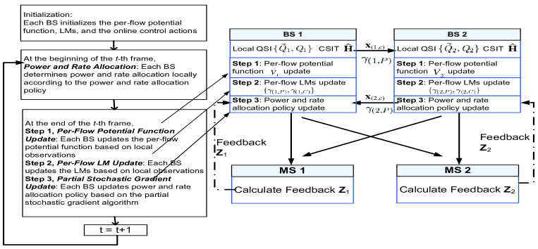
Figure 3: The system procedure of the proposed low-complexity distributed solution involving Alg. 1 and Alg. 2 with $K=2$.

Algorithm 1

(Distributed Online Learning Algorithm for Per-Flow Potential Functions and LMs) At each frame $t$, let $\widetilde{Q}_{k}$, $Q_{k}$ and $\hat{\mathbf{H}}$ be the observed post-decision QSI, pre-decision QSI and imperfect CSIT. Each BS $k$ updates its per-flow potential functions and LMs according to the following online learning update:

$$\begin{cases}&V_{k}^{t+1}(\widetilde{Q}_{k})=V_{k}^{t}(\widetilde{Q}_{k})+\kappa_{v}(t)\left[g_{k}\left(\boldsymbol{\gamma}_{k}^{t},\hat{\boldsymbol{\chi}}_{k},\widetilde{\mathbf{P}}_{k}^{*},\widetilde{\mathbf{R}}_{k}^{*}\right)+V_{k}^{t}(Q_{k}-U_{k})-V_{k}^{t}(\widetilde{Q}_{k}^{0})-V_{k}^{t}(\widetilde{Q}_{k})\right]\\ &\gamma_{(k,P)}^{t+1}=\Gamma\left[\gamma_{(k,P)}^{t}+\kappa_{\gamma}(t)({\color[rgb]{0,0,0}\widetilde{P}_{k}^{*}}-P_{k}^{0})\right]\\ &\gamma_{(k,C)}^{t+1}=\Gamma\left[\gamma_{(k,C)}^{t}+\kappa_{\gamma}(t)({\color[rgb]{0,0,0}\widetilde{R}_{k,c}^{*}}-R_{(k,c)}^{0})\right]\end{cases},$$ (31)

where $\hat{\boldsymbol{\chi}}_{k}=\{Q_{k},\hat{\mathbf{H}}\}$ and $U_{k}$ is the goodput to MS $k$ given by (18) under $\hat{\mathbf{H}}=\mathbf{H}$. $\{\widetilde{\mathbf{P}}_{k}^{*},\widetilde{\mathbf{R}}_{k}^{*}\}=\widetilde{\Omega}_{k}^{*}(\hat{\boldsymbol{\chi}}_{k})$. $\widetilde{P}_{k}^{*}$ and $\widetilde{R}_{k,c}^{*}$ are the power and backhaul consumption of BS $k$ given by $\widetilde{\Omega}_{k}^{*}(\hat{\boldsymbol{\chi}}_{k})$. $\Gamma[\cdot]$ is the projection onto an interval $[0,B]$ for some large constant $B>0$. $\{\kappa_{v}(t)\}$ and $\{\kappa_{\gamma}(t)\}$ are the step size sequences satisfying the following conditions: $\kappa_{v}(t)\geq 0,\sum_{t}\kappa_{v}(t)=\infty,\ \kappa_{\gamma}(t)\geq 0,\sum_{t}\kappa_{\gamma}(t)=\infty,\sum_{t}((\kappa_{v}(t))^{2}+(\kappa_{\gamma}(t))^{2})<\infty,\frac{\kappa_{\gamma}(t)}{\kappa_{v}(t)}\to 0.$  ∎

Remark 5 (Features of Algorithm 1)

Algorithm 1 only requires local observations of $\{\widetilde{Q}_{k},Q_{k}\}$ and $\hat{\mathbf{H}}$ at each BS $k$. Furthermore, both the per-flow potential functions and the LMs are updated simultaneously and distributively at each BS.   ∎

In the following, we establish the convergence proof of Algorithm 1. For given per-flow potential function vector $\mathbf{V}_{k}=\left(V_{k}(\widetilde{Q}_{k})\right)_{\widetilde{Q}_{k}=0,1,\cdots,N_{Q}}$ and LMs $\boldsymbol{\gamma}_{k}$, define a mapping $T_{k}:\mathbb{R}^{N_{Q}+1}\to\mathbb{R}$ for the post-decision state $\widetilde{Q}_{k}$ as follows: $T_{k}(\widetilde{Q}_{k};\boldsymbol{\gamma}_{k},\mathbf{V}_{k})=\text{R.H.S. of \eqref{eq:bellman_perflow}}$. Denote $\mathbf{T}_{k}(\boldsymbol{\gamma}_{k},\mathbf{V}_{k})=\left(T_{k}(\widetilde{Q}_{k};\boldsymbol{\gamma}_{k}),\mathbf{V}_{k}\right)_{\widetilde{Q}_{k}=0,1,\cdots,N_{Q}}$. Since we have two different step size sequences $\{\kappa_{v}(t)\}$ and $\{\kappa_{\gamma}(t)\}$ with $\kappa_{\gamma}(t)=o(\kappa_{v}(t))$, the per-flow potential function updates and the LM updates are done simultaneously but over two different timescales. The convergence analysis can be established over two timescales separately. Specifically, during the per-flow potential function update (timescale I), we have $\gamma_{(k,C)}^{t+1}-\gamma_{(k,C)}^{t}=O(\kappa_{\gamma}(t))=o(\kappa_{v}(t))$ and $\gamma_{(k,P)}^{t+1}-\gamma_{(k,P)}^{t}=O(\kappa_{\gamma}(t))=o(\kappa_{v}(t))$ for all $k\in\mathcal{K}$. Therefore, the LMs appear to be quasi-static during the per-flow potential function update in (31)[26, Chap. 6].

Lemma 3 (Convergence of Per-flow Potential Function Update (Timescale I))

For given $\boldsymbol{\gamma}_{k}$, the iterations of the per-flow potential functions $\mathbf{V}_{k}^{t}$ in Algorithm 1 converge almost surely to the fixed point of the per-flow fixed point equation in (30), i.e., $\lim_{t\rightarrow\infty}\mathbf{V}_{k}^{t}=\mathbf{V}_{k}^{\infty}$ for all $k\in\mathcal{K}$, where $V_{k}^{\infty}(\widetilde{Q}_{k})$ satisfies:

$$\mathbf{V}_{k}^{\infty}+V_{k}^{\infty}(\widetilde{Q}_{k}^{0})\mathbf{e}=\mathbf{T}_{k}(\boldsymbol{\gamma}_{k},\mathbf{V}_{k}^{\infty}).$$ (32)

$\mathbf{e}$ denotes the $(N_{Q}+1)$-dimension vector with all-one elements.

Proof:

The proof can be extended from[25, Chap. 3] and is omitted due to page limit. ∎

During the LM update (timescale II), we have $\lim_{t\to\infty}|V_{k}^{t}-V_{k}^{\infty}(\boldsymbol{\gamma}_{k}^{t})|=0$ w.p.1. for all $k\in\mathcal{K}$ [26, Chap. 6]. Hence, during the LM update in (31), the per-flow potential functions can be seen as almost equilibrated. The convergence of the LM update is summarized below.

Lemma 4 (Convergence of LM Update (Timescale II))

The iterations of the LMs $\boldsymbol{\gamma}^{t}=\{\gamma_{(k,P)}^{t},\gamma_{(k,C)}^{t}:k\in\mathcal{K}\}$ in Algorithm 1 converge almost surely to the invariant set:

$$\mathcal{S}_{\gamma}\triangleq\left\{\boldsymbol{\gamma}:||\boldsymbol{\gamma}-\boldsymbol{\gamma}^{*}||^{2}-\delta_{1}-\delta_{2}\leq 0\right\},$$ (33)

as $t\to\infty$, for some positive constants $\delta_{1}=O(P_{\text{cct}}^{2})$ and $\delta_{2}=O(\epsilon^{2})$, where $\epsilon=\sup_{\{\mathbf{H},\hat{\mathbf{H}}:\mathbf{H}\neq\hat{\mathbf{H}}\}}\Pr\{\mathbf{H}|\hat{\mathbf{H}}\}$ denotes the CSIT quality. $\boldsymbol{\gamma}^{*}=\{\gamma_{(k,P)}^{*},\gamma_{(k,C)}^{*}:k\in\mathcal{K}\}$ is the dual optimal solution to the dual problem in (25).   ∎

Proof:

Please refer to Appendix E. ∎

VI-C Distributed Online Power and Rate Control via Stochastic Partial Gradient Algorithm

Substituting (29) into the R.H.S. of (27), the control policy under linear approximation in (29) can be obtained by solving the following per-stage optimization problem.

Problem 2 (Per-Stage Optimization)

For any given LMs $\boldsymbol{\gamma}$, under the linear approximation in (29), the online control action (for an observed state realization $\hat{\boldsymbol{\chi}}$) is given by:

$$\begin{array}[]{l}{\color[rgb]{0,0,0}\hat{\Omega}^{*}(\hat{\boldsymbol{\chi}})=\{\hat{\Omega}_{P}^{*}(\hat{\boldsymbol{\chi}}),\hat{\Omega}_{R}^{*}(\hat{\boldsymbol{\chi}})\}}=\operatorname*{\arg\min}\limits_{\mathbf{P},\mathbf{R}}h^{\hat{\boldsymbol{\chi}}}(\mathbf{P},\mathbf{R})\end{array}$$ (34)

where $h^{\hat{\boldsymbol{\chi}}}(\mathbf{P},\mathbf{R})=\sum_{k\in\mathcal{K}}\mathbb{E}\Big{[}\gamma_{(k,P)}\big{(}P_{k}^{tx}+P_{\text{cct}}\mathbf{1}(P_{k}^{tx}>0)\big{)}+\gamma_{(k,C)}R_{(k,c)}+\overline{\mathbf{1}}_{(k,c)}\overline{\mathbf{1}}_{(k,p)}V_{k}\big{(}Q_{k}\big{)}+\mathbf{1}_{(k,c)}\mathbf{1}_{(k,p)}V_{k}\big{(}Q_{k}-R_{k}\big{)}+\overline{\mathbf{1}}_{(k,c)}\mathbf{1}_{(k,p)}V_{k}\big{(}Q_{k}-R_{(k,p)})\big{)}+\mathbf{1}_{(k,c)}\overline{\mathbf{1}}_{(k,p)}V_{k}\big{(}Q_{k}-R_{(k,c)}\big{)}\Big{|}\hat{\mathbf{H}}\Big{]}$. $\mathbf{1}_{(k,c)}=\mathbf{1}\big{(}R_{(k,c)}\leq C_{(k,c)}\big{)}$ and $\overline{\mathbf{1}}_{(k,c)}=1-\mathbf{1}_{(k,c)}$. $\mathbf{1}_{(k,p)}$ and $\overline{\mathbf{1}}_{(k,p)}$ are defined in a similar way.  ∎

Problem 2 is not tractable as $h^{\hat{\boldsymbol{\chi}}}(\mathbf{P},\mathbf{R})$ is not differentiable due to the indicator functions. To solve Problem 2, we first use the logistic function $f^{\eta}(x,y)=\frac{1}{1+e^{(x-y)\eta}}$ as a smooth approximation for the indicator function $\mathbf{1}(x\leq y)$ in (34), i.e., $f^{\eta}(x,y)\approx\mathbf{1}(x\leq y),\forall x,y\in\mathbb{R}^{+}$ [27, Chap. 3], [28, Chap. 1]. Note that the approximation is asymptotically accurate as $\eta\to\infty$. Then, we apply the gradient search method. Specifically, the gradient of $h^{\hat{\boldsymbol{\chi}}}(\mathbf{P},\mathbf{R})$ w.r.t. a control action $a_{k}\in\{P_{(k,c)}^{i},P_{(k,p)}^{i},R_{(k,c)},R_{(k,p)}:\forall i\}$ of BS $k$ is given by:

$$\frac{\partial h^{\hat{\boldsymbol{\chi}}}\left(\mathbf{P},\mathbf{R}\right)}{\partial a_{k}}$$ (35)

$$\approx \mathbb{E}\Big{[}\underbrace{\frac{\partial\big{[}\gamma_{(k,P)}(P_{k}^{tx}+P_{\text{cct}}f^{\eta}(0,P_{k}^{tx}))+\gamma_{(k,C)}R_{(k,c)}\big{]}}{\partial a_{k}}+\frac{\partial g_{k}^{\hat{\boldsymbol{\chi}}}(\mathbf{P},\mathbf{R}_{k},\mathbf{H},\mathbf{V}_{k})}{\partial a_{k}}+{\color[rgb]{0,0,0}\sum_{n\in\mathcal{K},n\neq k}}\frac{\gamma_{(n,p)}P_{(k,c),n}}{\partial a_{k}}}_{\text{$\triangleq y(a_{k})$, stochastic partial gradient}}$$

$$+\underbrace{{\color[rgb]{0,0,0}\sum_{n\in\mathcal{K},n\neq k}}\left(\gamma_{(n,p)}P_{\text{cct}}\frac{\partial f^{\eta}(0,P_{n}^{tx})}{\partial a_{k}}+\frac{\partial g_{n}^{\hat{\boldsymbol{\chi}}}(\mathbf{P},\mathbf{R}_{n},\mathbf{H},\mathbf{V}_{k})}{\partial a_{k}}\right)}_{\text{unknown to BS $k$}}\Big{|}\hat{\mathbf{H}}\Big{]},$$

$$g_{k}^{\hat{\boldsymbol{\chi}}}\left(\mathbf{P},\mathbf{R}_{k},\mathbf{H},\mathbf{V}_{k}\right)= \left(1-f^{\eta}\left(R_{(k,c)},C_{(k,c)}\right)\right)\left(1-f^{\eta}\left(R_{(k,p)},C_{(k,p)}\right)\right)V_{k}\left(Q_{k}\right)$$

$$+\left(1-f^{\eta}\left(R_{(k,c)},C_{(k,c)}\right)\right)f^{\eta}\left(R_{(k,p)},C_{(k,p)}\right)V_{k}\left(Q_{k}-R_{(k,p)}\right)$$

$$+f^{\eta}\left(R_{(k,c)},C_{(k,c)}\right)\left(1-f^{\eta}\left(R_{(k,p)},C_{(k,p)}\right)\right)V_{k}\left(Q_{k}-R_{(k,c)}\right)$$

$$+f^{\eta}\left(R_{(k,c)},C_{(k,c)}\right)f^{\eta}\left(R_{(k,p)},C_{(k,p)}\right)V_{k}\left(Q_{k}-R_{k}\right).$$

The gradient $\frac{\partial h^{\hat{\boldsymbol{\chi}}}\left(\mathbf{P},\mathbf{R}\right)}{\partial a_{k}}$ in (35) cannot be calculated locally at each BS due to the following reasons. First, the second term in (35) is unknown to BS $k$ under the distributed implementation requirement. Second, the expectation $\mathbb{E}$ cannot be computed at BS $k$ without knowledge of the CSIT error kernels under Assumption 2. In the following, we propose a distributed online stochastic partial gradient algorithm to obtain the power and rate control.

Algorithm 2

[Distributed Online Stochastic Partial Gradient Algorithm for Power and Rate Control] At each frame $t$, let $\hat{\boldsymbol{\chi}}_{k}=\{Q_{k},\hat{\mathbf{H}}\}$ denote the observation at each BS $k$. Each BS $k$ takes control actions $a_{k}^{t}(\hat{\boldsymbol{\chi}}_{k})$, obtains $\{\gamma_{(n,P)}^{t}:n\in\mathcal{K},n\neq k\}$ from other BSs through backhaul, and updates the control according to the following stochastic partial gradient update:

$$a_{k}^{t+1}(\hat{\boldsymbol{\chi}}_{k})=\left[a_{k}^{t}(\hat{\boldsymbol{\chi}}_{k})-{\color[rgb]{0,0,0}\kappa_{a}(t)}y\left(a_{k}^{t}(\hat{\boldsymbol{\chi}}_{k})\right)\right]^{+},$$ (36)

where $a_{k}\in\{P_{(k,c)}^{i},P_{(k,p)}^{i},R_{(k,c)},R_{(k,p)}:\forall i\}$ and $\{{\color[rgb]{0,0,0}\kappa_{a}(t)}\}$ is the step size sequence satisfying the following conditions: ${\color[rgb]{0,0,0}\kappa_{a}(t)}\geq 0,\sum_{t}{\color[rgb]{0,0,0}\kappa_{a}(t)}=\infty,\sum_{t}({\color[rgb]{0,0,0}{\color[rgb]{0,0,0}\kappa_{a}(t)}})^{2}<\infty.$   ∎

Table II illustrates the detailed expressions of $y(a_{k}^{t})$ in (36) at frame $t$.

Control Actions $a_{k}^{t}$	Stochastic Partial Gradient $y(a_{k}^{t})$
$P_{(k,p)}^{i,t}$	$\gamma_{(k,P)}^{t}+\gamma_{(k,P)}^{t}P_{\text{cct}}\frac{\partial f^{\eta}(0,P_{k}^{tx,t})}{\partial P_{(k,p)}^{i,t}}+\frac{\partial g_{k}^{\hat{\boldsymbol{\chi}}}(\mathbf{P}^{t},\mathbf{R}_{k}^{t},\mathbf{H},\mathbf{V}_{k}^{t})}{\partial P_{(k,p)}^{i,t}}$
$R_{(k,p)}^{t}$	$\frac{\partial g_{k}^{\hat{\boldsymbol{\chi}}}(\mathbf{P}^{t},\mathbf{R}_{k}^{t},\mathbf{H},\mathbf{V}_{k}^{t})}{\partial R_{(k,p)}^{t}}$
$P_{(k,c)}^{i,t}$	$\gamma_{(k,P)}^{t}\alpha_{(k,k)}^{i}+\sum_{n\in\mathcal{K},n\neq k}\gamma_{(n,P)}^{t}\alpha_{(k,n)}^{i}+\gamma_{(k,P)}^{t}P_{\text{cct}}\frac{\partial f^{\eta}(0,P_{k}^{tx,t})}{\partial P_{(k,c)}^{i,t}}+\frac{\partial g_{k}^{\hat{\boldsymbol{\chi}}}(\mathbf{P}^{t},\mathbf{R}_{k}^{t},\mathbf{H},\mathbf{V}_{k}^{t})}{\partial P_{(k,c)}^{i,t}}$
$R_{(k,c)}^{t}$	$\gamma_{(k,C)}^{t}+\frac{\partial g_{k}^{\hat{\boldsymbol{\chi}}}(\mathbf{P}^{t},\mathbf{R}_{k}^{t},\mathbf{H},\mathbf{V}_{k}^{t})}{\partial R_{(k,c)}^{t}}$

TABLE II: Expressions of $y(a_{k}^{t})$ at frame $t$ for specific control actions.

The following lemma summarizes the convergence of Algorithm 2.

Lemma 5 (Convergence of Algorithm 2)

Let $\hat{\mathcal{W}}^{*}$ be the set of local minimum points $\hat{\mathbf{W}}^{*}=\{\hat{\mathbf{P}}^{*},\hat{\mathbf{R}}^{*}\}$ of Problem 2. The iterations for $\mathbf{W}^{t}=\{\mathbf{P}^{t},\mathbf{R}^{t}\}$ in Algorithm 2 converge almost surely to the invariant set:

$$\mathcal{S}_{w}\triangleq\left\{\mathbf{W}:||\mathbf{W}-\hat{\mathbf{W}}^{*}||^{2}-\delta_{1}-\delta_{2}\leq 0\right\},$$ (37)

as $t\to\infty$, for some local minimum point $\hat{\mathbf{W}}^{*}\in\hat{\mathcal{W}}^{*}$ and positive constants $\delta_{1}=O(P_{\text{cct}}^{2})$ and $\delta_{2}=O(\epsilon^{2})$, where $\epsilon=\sup_{\{\mathbf{H},\hat{\mathbf{H}}:\mathbf{H}\neq\hat{\mathbf{H}}\}}\Pr\{\mathbf{H}|\hat{\mathbf{H}}\}$ denotes the CSIT quality.   ∎

Proof:

Please refer to Appendix F. ∎

By Lemma 5, Algorithm 2 gives the asymptotically local optimal solution at small CSIT errors and $P_{\text{cct}}$.

Finally, we discuss the implementation of Algorithm 2 in practical systems.

Remark 6 (Generalized ACK/NAK as MS Feedback for Algorithm 2)

At each BS $k$, to compute the stochastic partial gradients in Table II, some terms in $\frac{\partial g_{k}^{\hat{\boldsymbol{\chi}}}(\mathbf{P}^{t},\mathbf{R}_{k}^{t},\mathbf{H},\mathbf{V}_{k}^{t})}{\partial a_{k}^{t}}$ regarding $C_{(k,c)}^{t}$ and $C_{(k,p)}^{t}$ have to be fed back from MS $k$. Utilizing the property of the logistic function at large $\eta$, the MS feedback can be substantially simplified. Specifically, for large $\eta$, we have

$$f^{\eta}(x,y))=\frac{1}{1+e^{(x-y)\eta}}\approx\mathbf{1}(x\leq y),\quad J(x-y)\triangleq\frac{-\eta e^{(x-y)\eta}}{(1+e^{(x-y)\eta})^{2}}\approx\frac{\eta}{5}\mathbf{1}\big{(}|x-y|\leq\frac{2}{\eta}\big{)}.$$

Note that the approximations are asymptotically accurate as $\eta\to\infty$. As a result, we have

$$\frac{\partial f^{\eta}(R_{(k,c)},C_{(k,c)})}{\partial R_{(k,c)}}= J(R_{(k,c)}-C_{(k,c)})\approx\frac{\eta}{5}\mathbf{1}\big{(}|R_{(k,c)}-C_{(k,c)}|\leq\frac{2}{\eta}\big{)}$$

$$\frac{\partial f^{\eta}(R_{(k,c)},C_{(k,c)})}{\partial P_{(k,c)}^{i}}= J(R_{(k,c)}-C_{(k,c)})\frac{\sigma_{(k,c)}^{i}}{(1+\sigma_{(k,c)}^{i}P_{(k,c)}^{i}+I_{(k,c)}^{i})\text{ln}2}\approx\frac{\eta}{5}\mathbf{1}\big{(}|R_{(k,c)}-C_{(k,c)}|\leq\frac{2}{\eta}\big{)}$$

Similar notations can be defined for the private streams with $c$ replaced by $p$. Based on these approximations, MS $k$ only needs to feed back a binary vector

$$\mathbf{Z}_{k}=\left\{\mathbf{1}(R_{(k,c)}^{t}\leq C_{(k,c)}^{t}),\mathbf{1}\big{(}|R_{(k,c)}^{t}-C_{(k,c)}^{t}|\leq\frac{2}{\eta}\big{)},\mathbf{1}(R_{(k,p)}^{t}\leq C_{(k,p)}^{t}),\mathbf{1}\big{(}|R_{(k,p)}^{t}-C_{(k,p)}^{t}|\leq\frac{2}{\eta}\big{)}\right\}$$

at each frame $t$ in order for BS $k$ to compute the stochastic partial gradients. This binary feedback has low overhead. In addition, there are existing built-in mechanisms in most wireless systems for these ACK/NAK types of feedback from MSs. Furthermore, the convergence property of Algorithm 2 (Lemma 5) holds even under the approximations.  ∎

Remark 7 (Features of of Algorithm 2)

Algorithm 2 only requires local observations $\{\hat{\boldsymbol{\chi}}_{k},\mathbf{Z}_{k}\}$ and local potential functions $\mathbf{V}_{k}$ at each BS $k$, and hence, can be implemented distributively. In addition, explicit knowledge of the CSIT error kernel is not required, and hence, Algorithm 2 is robust against uncertainty in the modeling.  ∎

VII Simulation and Discussion

In this section, we compare the performance of the proposed distributed solution with various baseline schemes using numerical simulations. The average performance is evaluated over $10^{6}$ iterations. At each frame $t$, we assume the CSI $\mathbf{H}_{kn}(t)$ is uniformly distributed over a state space $\mathcal{H}^{N\times M}$ of size $|\mathcal{H}^{N\times M}|=20$. We consider Poisson packet arrival with average arrival rate $\lambda_{k}$ (packet/s) and exponentially distributed random packet size with mean $\overline{N}_{k}=5$Mbits for $k\in\{1,2\}$. The buffer size $N_{Q}$ is 54Mbits. The scheduling frame duration $\tau$ is 5ms. The total BW is $W=10$MHz. We consider the CSIT error model with CSIT error variance $\sigma_{e}=0.15$[29]. The number of transmit and receive antennas is given by $\{M=3,N=2\}$, the number of common and private streams for the Pco-MIMO scheme is $\{d_{(k,c)}=1,d_{(k,p)}=1\}$, $f_{k}(Q_{k})=Q_{k}$, and $\beta_{k}=1$ for all $k\in\mathcal{K}$. We choose $P_{1}^{0}=P_{2}^{0}$ and $C_{1}^{0}=C_{2}^{0}$.

We consider four baseline schemes: Baseline 1 (Coordinative MIMO)[1], Baseline 2 (Uco-MIMO)[10], Baseline 3 (Full Cooperative MIMO)[6], and Baseline 4 (Channel-Aware Pco-MIMO). Remark 1 illustrates the details of the precoder and decorrelator designs in Baselines 1, 2 and 3. Baseline 4 adopts the proposed Pco-MIMO PHY scheme in the precoder and decorrelator design. All the baseline schemes maximize system throughput under the same backhaul and power constraints as the proposed scheme. Therefore, the resulting resource control designs are adaptive to CSIT only, i.e., channel-aware. Specifically, these four baseline schemes treat the imperfect CSIT as perfect information and do not consider rate allocation due to imperfect CSIT. But Baselines 2, 3, and 4 still consider rate allocation for common streams due to the average backhaul constraints. All the baseline schemes consider power allocation.

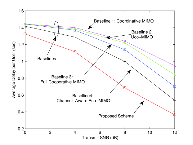
(a) Average delay per user versus maximum transmit SNR $P_{k}^{0}$. $R_{(k,c)}^{0}=1.1W\tau\log_{2}(1+P_{k}^{0})$ (bits/frame), $P_{\text{cct}}=20$dBm, and $\lambda_{k}=6$ (packet/s).

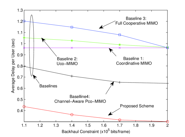
(b) Average delay per user versus maximum backhaul consumption $R_{(k,c)}^{0}$. $P_{k}^{0}=12$dB, $P_{\text{cct}}=20$dBm, and $\lambda_{k}=7$ (packet/s).

Figure 4: Average delay per user versus maximum transmit SNR and backhaul consumption.

VII-A Delay Performance w.r.t. Transmit SNR

Fig. 4 (a) illustrates the average delay per user versus the maximum transmit SNR $P_{k}^{0}$. The average delay of all the schemes decreases as the transmit SNR increases. This figure demonstrates the medium backhaul consumption regime, in which Baseline 3 (Full Cooperative MIMO) outperforms Baseline 1 (Coordinative MIMO), while full cooperative MIMO is not the best choice. The performance gain of Baseline 4 (Channel-Aware Pco-MIMO) compared with Baseline 3 (Full Cooperative MIMO) is contributed by the proposed flexible cooperation level adjustment according to the backhaul consumption requirement. Both Baseline 4 and the proposed scheme apply the proposed Pco-MIMO scheme. The performance gain of the proposed solution compared with Baseline 4 is contributed by the careful delay-aware dynamic power and rate allocation with the consideration of the imperfect CSIT. It can be seen that the proposed scheme has significant performance gain compared with all the baselines.

VII-B Delay Performance w.r.t. Backhaul Consumption

Fig. 4 (b) illustrates the average delay per user versus the maximum backhaul consumption $R_{(k,c)}^{0}$. The average delay of all the schemes decreases as the backhaul consumption increases. This figure demonstrates the small backhaul consumption regime, in which Baseline 1 (Coordinative MIMO) outperforms Baseline 3 (Full Cooperative MIMO). By carefully making use of the very limited backhaul resources with the proposed flexible cooperation level adjustment, Baseline 4 (Channel-Aware Pco-MIMO) outperforms Baseline 1. In addition, similar comparisons between Baseline 4 and the proposed solution (as in Section VII-A) can be made. It can be observed that the proposed scheme has significant performance gain compared with all the baselines. Note that the delay performance of Baseline 1 is independent of the backhaul constraint as no data sharing is needed in coordinated beamforming.

VII-C Convergence Performance

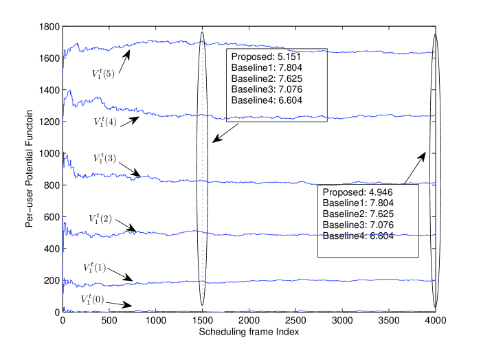
(a) Per User Potential Function

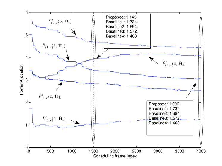
(b) Power Allocation

Figure 5: Convergence property of the proposed scheme. $P_{k}^{0}=4$dB, $P_{\text{cct}}=20$dBm, $R_{(k,c)}^{0}=1.1W\tau\log_{2}(1+P_{k}^{0})$ (bits/frame), and $\lambda_{k}=4.5$ (packet/s). For illustration, we randomly generate a CSIT realization and plot the power allocation trajectories for different QSI and the randomly generated CSIT realization.

Fig. 5 illustrates the convergence property of the proposed scheme. It can be observed that the convergence rate of the online algorithm is quite fast. For example, the delay performance at 1500-th scheduling frame is already quite close to the converged average delay.

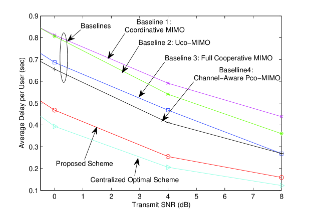
(a) Average delay per user versus transmit SNR $P_{k}^{0}$.

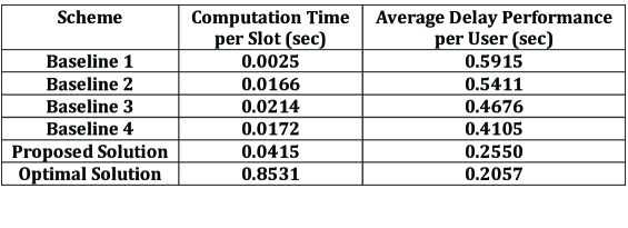
(b) Matlab computation time per slot and average delay performance per user at $P_{k}^{0}=0$dB.

Figure 6: Performance and computational complexity. $R_{(k,c)}^{0}=W\tau\log_{2}(1+P_{k}^{0})$ (bits/frame), $P_{\text{cct}}=10$dBm, $N_{Q}=18$Mbits.

VII-D Computational Complexity

The computational complexity of the proposed solution is of the same order ($O(K)$) as the four baseline schemes, while it has much lower complexity than the optimal solution ($O(N_{Q}^{K})$). Fig. 6 (a) and Fig. 6 (b) illustrate the performance and computational complexity comparisons between the baseline schemes, the proposed distributed solution and the centralized optimal solution.

VIII Summary

In this paper, we first propose a novel flexible Pco-MIMO PHY scheme. Based on the Pco-MIMO scheme, we formulate the delay-optimal control problem as an infinite horizon average cost CPOMDP. We obtain an equivalent Bellman equation to solve the CPOMDP. To facilitate implementation, we propose a low-complexity distributed solution. We prove the convergence and the asymptotical optimality of the proposed solution.

Appendix A: Proof of Theorem 1

When CSIT is perfect and $\{d_{(k,c)},d_{(k,p)}:k\in\mathcal{K}\}$ satisfies the conditions in (4), there is no interference under the Pco-MIMO scheme. Therefore, the system DoF is given by the total number of non-interfering streams, i.e., $\text{DoF}(\text{Pco-MIMO})=\sum_{k\in\mathcal{K}}(d_{(k,p)}+d_{(k,c)})$. From the second constraint in (4), we have:

$$\left(d_{(k,c)}+\sum_{n\in\mathcal{K}}d_{(n,p)}\right)+\sum_{n\in\mathcal{K},n\neq k}d_{(n,c)}\leq N+(K-1)d_{K,M,N}+\sum_{n\in\mathcal{K},n\neq k}d_{(n,c)},\forall k\in\mathcal{K},$$ (38)

where the above equality holds if $d_{(k,c)}+\sum_{n\in\mathcal{K}}d_{(n,p)}=N+(K-1)d_{K,M,N}$. Since (38) holds for all $k\in\mathcal{K}$, we can prove (13) and (14). Furthermore, by (5) for all $k\in\mathcal{K}$, we can show $\text{DoF}_{\max}(\text{Pco-MIMO})\leq N+(K-1)d_{K,M,N}+(K-1)(N-d_{K,M,N})=KN$, where the equality holds when (15) is satisfied.

Appendix B: Proof of Theorem 2

First, we prove Statement (a). Problem (26) can be expressed as an equivalent MDP: $\min_{\Omega}\lim\sup_{T\rightarrow\infty}\frac{1}{T}\sum\nolimits_{t=1}^{T}\mathbb{E}^{\Omega}\left[\mathbb{E}[g(\boldsymbol{\gamma},\boldsymbol{\chi},\Omega(\hat{\boldsymbol{\chi}}))|\mathbf{Q}]\right]$ with a tuple of the following four objects: the state space $\{\mathbf{Q}\}$; the action space $\{\Omega(\mathbf{Q})\}$, where $\Omega(\mathbf{Q})=\{\Omega(\hat{\boldsymbol{\chi}}):\forall\hat{\mathbf{H}}\}$; the transition kernel $\Pr\{\widetilde{\mathbf{Q}}^{\prime}|\mathbf{Q},\Omega(\mathbf{Q})\}=\mathbb{E}\left[\Pr\{\widetilde{\mathbf{Q}}^{\prime}|\boldsymbol{\chi},\Omega(\hat{\boldsymbol{\chi}})\}|\mathbf{Q}\right]$; and the per-stage cost function $\widetilde{g}(\boldsymbol{\gamma},\mathbf{Q},\Omega(\mathbf{Q}))=\mathbb{E}[g(\boldsymbol{\gamma},\boldsymbol{\chi},\Omega(\hat{\boldsymbol{\chi}}))|\mathbf{Q}]$. By standard MDP techniques, we know that the optimal policy $\Omega^{*}$ can be obtained by solving the equivalent Bellman equation in (27) [13, Chap. 4]. Next, we prove Statement (b). By Theorem 2.1 in [16], the support of the randomized policy to the equivalent MDP is included in the set of the optimal solutions:

$$\arg\min_{\mathbf{P},\mathbf{R}}\mathbb{E}\left[g(\boldsymbol{\gamma},\boldsymbol{\chi},\mathbf{P},\mathbf{R})+\sum\nolimits_{\widetilde{\mathbf{Q}}^{\prime}}\Pr\{\widetilde{\mathbf{Q}}^{\prime}|\boldsymbol{\chi},\mathbf{P},\mathbf{R}\}V(\widetilde{\mathbf{Q}}^{\prime})\bigg{|}\hat{\boldsymbol{\chi}}\right]$$

Hence, if the set of the optimal solutions is a singleton set for all $\hat{\boldsymbol{\chi}}$, there is no loss of optimality to focus on deterministic policies. Thus, the deterministic policy $\Omega^{*}$ is optimal.

Appendix C: Proof of Lemma 1

First, we show that the duality gap is zero over the stationary randomized policy space. Define a stationary randomized policy $\bar{\Omega}$, which is a mapping from the observed state $\hat{\boldsymbol{\chi}}$ to some measurable $f:\mathcal{S}\to\mathcal{P}(\mathcal{U})$, where $\mathcal{S}$ is the observed state space, $\mathcal{U}$ is the power and rate allocation space, and $\mathcal{P}$ is the Polish space of probability measures on $\mathcal{U}$ with the Prohorov topology[30, Chap. 2]. The observed state $\hat{\boldsymbol{\chi}}=\{\mathbf{Q},\hat{\mathbf{H}}\}$ under the randem control of the unichain policy $\bar{\Omega}$ has an invariant probability measure $\pi\in\mathcal{P}(\mathcal{S})$. The ergodic occupation measure $\pi_{{\color[rgb]{0,0,0}\bar{\Omega}}}$ associated with the pair $(\pi,{\color[rgb]{0,0,0}\bar{\Omega}})$ is defined by[31]:

$$\int_{\mathcal{S}\times\mathcal{U}}g(\hat{\boldsymbol{\chi}},y)\text{d}\pi_{{\color[rgb]{0,0,0}\bar{\Omega}}}=\sum\nolimits_{\hat{\boldsymbol{\chi}}\in\mathcal{S}}\pi(\mathcal{S})\int_{\mathcal{U}}g(\hat{\boldsymbol{\chi}},y)f(\hat{\boldsymbol{\chi}},\text{d}y),$$ (39)

where $g(\hat{\boldsymbol{\chi}},y)$ is the per stage cost function given the observed state is $\hat{\boldsymbol{\chi}}$ and action $y$ is taken. Let $\mathcal{G}$ denote the set of all ergodic occupation measures $\pi_{{\color[rgb]{0,0,0}\bar{\Omega}}}$, and it has been shown in [31] that $\mathcal{G}$ is closed convex in $\mathcal{P}(\mathcal{S}\times\mathcal{U})$. Therefore, the primal Problem 1 can be recast as a convex problem given by:

$$\begin{array}[]{lll}\min_{\nu\in\mathcal{G}}&\int g(\hat{\boldsymbol{\chi}},y)\text{d}\nu\\ \text{s.t.}&\int P_{k}(\hat{\boldsymbol{\chi}},y)\text{d}\nu\leq P_{k}^{0};\quad\int R_{(k,c)}(\hat{\boldsymbol{\chi}},y)\text{d}\nu\leq R_{(k,c)}^{0},\forall k\end{array},$$ (40)

which is an infinite dimensional linear program [31], [32, Chap. 1]. Define the Lagrangian function: $L_{\text{LP}}(\nu,\boldsymbol{\gamma})=\int g\text{d}\nu+\sum_{k}\gamma_{(k,P)}(\int P_{k}\text{d}\nu-P_{k}^{0})+\sum_{k}\gamma_{(k,C)}(\int R_{(k,c)}\text{d}\nu-R_{(k,c)}^{0}).$ We have the saddle-point condition: $L_{\text{LP}}(\nu,\boldsymbol{\gamma}^{*})\geq L_{\text{LP}}(\nu^{*},\boldsymbol{\gamma}^{*})\geq L_{\text{LP}}(\nu^{*},\boldsymbol{\gamma})$, i.e., the duality gap is zero over the stationary randomized policy space.

Next, from Theorem 2 (b), there is no loss of optimality by focusing on deterministic policies given that the condition of Theorem 2 (b) holds. Hence, we have $\min_{\nu}L_{\text{LP}}(\nu,\boldsymbol{\gamma})=\min_{\Omega}L_{\beta}(\Omega,\boldsymbol{\gamma})$ for any $\boldsymbol{\gamma}\succeq 0$. As a result, the saddle point condition holds for the constrained Problem 1 over the domain of deterministic policies, i.e., $L_{\beta}(\Omega,\gamma^{*})\geq L_{\beta}(\Omega^{*},\gamma^{*})\geq L_{\beta}(\Omega^{*},\gamma)$ for all deterministic policies $\Omega$ and $\boldsymbol{\gamma}\succeq 0$. As a result, $(\Omega^{*},\gamma^{*})$ is the saddle point of $L_{\beta}(\Omega,\gamma)$ and the duality gap is zero, i.e., (28) holds.

Appendix D: Proof of Lemma 2

When $\hat{\mathbf{H}}=\mathbf{H}$, there is no interference under the Pco-MIMO. Thus, given $\hat{\boldsymbol{\chi}}=\boldsymbol{\chi}$ and $\{\mathbf{P},\mathbf{R}\}$, $\widetilde{Q}^{\prime}_{k}=Q_{k}-U_{k}(\hat{\mathbf{H}},\mathbf{P}_{k},\mathbf{R}_{k})$ is independent of $Q_{n}$ and $\{\mathbf{P}_{n},\mathbf{R}_{n}\}$ for all $n\in\mathcal{K},n\neq k$. Thus, we have $\Pr\{\widetilde{Q}_{k}^{\prime}|\hat{\boldsymbol{\chi}},\mathbf{P},\mathbf{R}\}=\Pr\{\widetilde{Q}_{k}^{\prime}|\hat{\boldsymbol{\chi}}_{k},\mathbf{P}_{k},\mathbf{R}_{k}\}.$ When $P_{\text{cct}}=0$, we have $g(\boldsymbol{\gamma},\hat{\boldsymbol{\chi}},\mathbf{P},\mathbf{R})=\sum_{k}g_{k}(\boldsymbol{\gamma}_{k},\hat{\boldsymbol{\chi}}_{k},\mathbf{P}_{k},\mathbf{R}_{k}).$ Suppose $V(\widetilde{\mathbf{Q}})=\sum_{k}V(\widetilde{Q}_{k})$ and $\theta=\sum_{k}V_{k}(\widetilde{Q}_{k}^{0})$. Then, the Bellman equation in (27) becomes:

$$\sum_{k}V_{k}(\widetilde{Q}_{k})+\sum_{k}V_{k}(\widetilde{Q}_{k}^{0})$$

$$= \mathbb{E}\left[\min_{\mathbf{P},\mathbf{R}}\left[g(\boldsymbol{\gamma},\boldsymbol{\chi},\mathbf{P},\mathbf{R})+\sum\nolimits_{\widetilde{\mathbf{Q}}^{\prime}}\Pr\{\widetilde{\mathbf{Q}}^{\prime}|\boldsymbol{\chi},\mathbf{P},\mathbf{R}\}\left(\sum_{k}V_{k}(\widetilde{Q}_{k}^{\prime})\right)\right]\Bigg{|}\widetilde{\mathbf{Q}}\right]$$

$$\stackrel{{\scriptstyle(a)}}{{=}} \mathbb{E}\left[\min_{\mathbf{P},\mathbf{R}}\left[\sum_{k}\left(g_{k}(\boldsymbol{\gamma}_{k},\hat{\boldsymbol{\chi}}_{k},\mathbf{P}_{k},\mathbf{R}_{k})+\sum_{\widetilde{Q}_{k}^{\prime}}\Pr\{\widetilde{Q}_{k}^{\prime}|\hat{\boldsymbol{\chi}}_{k},\mathbf{P}_{k},\mathbf{R}_{k}\}V_{k}(\widetilde{Q}_{k}^{\prime})\right)\right]\Bigg{|}\widetilde{\mathbf{Q}}\right]$$

$$\stackrel{{\scriptstyle(b)}}{{=}} \sum_{k}\mathbb{E}\left[\min_{\mathbf{P}_{k},\mathbf{R}_{k}}\left[g_{k}(\boldsymbol{\gamma}_{k},\hat{\boldsymbol{\chi}}_{k},\mathbf{P}_{k},\mathbf{R}_{k})+\sum_{\widetilde{Q}_{k}^{\prime}}\Pr\{\widetilde{Q}_{k}^{\prime}|\hat{\boldsymbol{\chi}}_{k},\mathbf{P}_{k},\mathbf{R}_{k}\}V_{k}(\widetilde{Q}_{k}^{\prime})\right]\Bigg{|}\widetilde{Q}_{k}\right],$$ (41)

where (a) is due to $\sum\nolimits_{\widetilde{\mathbf{Q}}^{\prime}}\Pr\{\widetilde{\mathbf{Q}}^{\prime}|\hat{\boldsymbol{\chi}},\mathbf{P},\mathbf{R}\}\left(\sum_{k}V_{k}(\widetilde{Q}_{k}^{\prime})\right)=\sum_{k}\sum\nolimits_{\widetilde{\mathbf{Q}}^{\prime}}\Pr\{\widetilde{\mathbf{Q}}^{\prime}|\hat{\boldsymbol{\chi}},\mathbf{P},\mathbf{R}\}V_{k}(\widetilde{Q}_{k}^{\prime})=\sum_{k}\sum\nolimits_{\widetilde{Q}_{k}^{\prime}}\Pr\{\widetilde{Q}_{k}^{\prime}|\hat{\boldsymbol{\chi}},\mathbf{P},\mathbf{R}\}V_{k}(\widetilde{Q}_{k}^{\prime})=\sum_{k}\sum\nolimits_{\widetilde{Q}_{k}^{\prime}}\Pr\{\widetilde{Q}_{k}^{\prime}|\hat{\boldsymbol{\chi}}_{k},\mathbf{P}_{k},\mathbf{R}_{k}\}V_{k}(\widetilde{Q}_{k}^{\prime})$ and (b) is due to the independent assumptions w.r.t. $k$ in the CSI model, imperfect CSI model and bursty source model. Therefore, (41) can be recast into per-flow Bellman equations given by (30) for each MS $k$. Furthermore, since the solution of the Bellman equation is unique up to a constant, we can conclude that when $V_{k}(\widetilde{Q}_{k})$ is a solution to the per-flow fixed point equation in (30), $V(\widetilde{\mathbf{Q}})=\sum_{k}V_{k}(\widetilde{Q}_{k})$ is a solution of the Bellman equation in (30).

Appendix E: Proof of Lemma 4

First, we obtain the ordinary differential equation (ODE) of the LM update in Algorithm 1. Due to the separation of timescales, the primal update of the potential function can be regarded as converged to $\mathbf{V}_{k}(\boldsymbol{\gamma}^{t})$ w.r.t. the current LMs $\boldsymbol{\gamma}^{t}$. Let $\widetilde{\Omega}^{*}=\{\widetilde{\Omega}_{k}^{*}:k\in\mathcal{K}\}$. Using the standard stochastic approximation argument in Lemma 1 of [26, Chap. 6], the dynamics of the LMs learning equation under $\widetilde{\Omega}^{*}(\boldsymbol{\gamma}(t))$) can be represented by the following ODE:

$$\dot{\boldsymbol{\gamma}}(t)=f_{\widetilde{\Omega}^{*}}(\boldsymbol{\gamma}(t)){\color[rgb]{0,0,0}\triangleq}\mathbb{E}^{\widetilde{\Omega}^{*}(\boldsymbol{\gamma}(t))}[\widetilde{P}_{1}^{*}(\boldsymbol{\gamma}(t))-P_{1}^{0},\widetilde{P}_{2}^{*}(\boldsymbol{\gamma}(t))-P_{2}^{0},\widetilde{R}_{(1,c)}^{*}(\boldsymbol{\gamma}(t))-C_{1}^{0},\widetilde{R}_{(2,c)}^{*}(\boldsymbol{\gamma}(t))-C_{2}^{0}]^{T},$$ (42)

where $\widetilde{P}_{k}^{*}(\boldsymbol{\gamma}(t))$ and $\widetilde{R}_{(k,c)}^{*}(\boldsymbol{\gamma}(t))$ are the power and backhaul consumption given by $\widetilde{\Omega}^{*}(\boldsymbol{\gamma}(t),\hat{\boldsymbol{\chi}})$. At the equilibrium point $\boldsymbol{\gamma}^{*}$ of the ODE (42), we have $\boldsymbol{\gamma}^{*}\cdot f_{\widetilde{\Omega}^{*}}(\boldsymbol{\gamma}^{*})=0$, which satisfies the power and backhaul consumption constraints in (20) and (21) (by KKT conditions).

Next, we consider the case when $\epsilon=0$ and $P_{\text{cct}}=0$. By Lemma 2, we have $\Omega^{*}=\widetilde{\Omega}^{*}$ when $\epsilon=0$ and $P_{\text{cct}}=0$. The ODE in (42) becomes:

$$\dot{\boldsymbol{\gamma}}(t)=f_{\Omega^{*}}(\boldsymbol{\gamma}(t)){\color[rgb]{0,0,0}\triangleq}\mathbb{E}^{\Omega^{*}(\boldsymbol{\gamma}(t))}[P^{*}_{1}(\boldsymbol{\gamma}(t))-P_{1}^{0},P^{*}_{2}(\boldsymbol{\gamma}(t))-P_{2}^{0},R^{*}_{(1,c)}(\boldsymbol{\gamma}(t))-C_{1}^{0},R^{*}_{(2,c)}(\boldsymbol{\gamma}(t))-C_{2}^{0}]^{T},$$ (43)

where $P_{k}^{*}(\boldsymbol{\gamma}(t))$ and $R_{(k,c)}^{*}(\boldsymbol{\gamma}(t))$ is the power and backhaul consumption given by $\Omega^{*}(\boldsymbol{\gamma}(t),\hat{\boldsymbol{\chi}})$. On the other hand, since $\Omega^{*}(\boldsymbol{\gamma})$ is optimal and $\epsilon=0$ and $P_{\text{cct}}=0$, we have $\Omega^{*}(\boldsymbol{\gamma})=\arg\min_{\Omega(\boldsymbol{\gamma})}\mathbb{E}^{\Omega(\boldsymbol{\gamma})}[\sum_{k}g_{k}(\boldsymbol{\gamma}_{k},\hat{\boldsymbol{\chi}}_{k},\Omega_{k}(\boldsymbol{\gamma},\hat{\boldsymbol{\chi}}_{k}))]$. Define $G(\boldsymbol{\gamma})=\mathbb{E}^{\Omega^{*}(\boldsymbol{\gamma})}[\sum_{k}g_{k}(\boldsymbol{\gamma}_{k},\hat{\boldsymbol{\chi}},\Omega_{k}^{*}(\boldsymbol{\gamma},\hat{\boldsymbol{\chi}})){\color[rgb]{0,0,0}]}$. By the envelope theorem, we have $\frac{\partial G(\boldsymbol{\gamma})}{\partial\gamma_{(k,P)}}=\mathbb{E}^{\Omega^{*}(\boldsymbol{\gamma})}[P^{*}_{k}(\boldsymbol{\gamma})-P_{k}^{0}]=\dot{\gamma}_{(k,P)}.$ Similarly, we have $\frac{\partial G(\boldsymbol{\gamma})}{\partial\gamma_{(k,C)}}=\mathbb{E}^{\Omega^{*}(\boldsymbol{\gamma})}[R^{*}_{(k,c)}(\boldsymbol{\gamma})-R_{(k,c)}^{0}]=\dot{\gamma}_{(k,C)}.$ Therefore, we can show that the ODE in (43) can be expressed as $\dot{\boldsymbol{\gamma}}(t)=\triangledown G(\boldsymbol{\gamma}(t))$. Since the dual function $G(\boldsymbol{\gamma})$ is a concave function, from the standard gradient update argument, the ODE in (43) will converge to the equilibrium point $\boldsymbol{\gamma}_{0}^{*}$. Thus, we have $\boldsymbol{\gamma}_{0}^{*}\cdot\triangledown G(\boldsymbol{\gamma}_{0}^{*})=0$. $\boldsymbol{\gamma}_{0}^{*}$ corresponds to the LMs associated with the power and backhaul constraints under the optimal policy (by KKT conditions). Furthermore, the equilibrium point $\boldsymbol{\gamma}_{0}^{*}$ is exponentially stable on $\mathcal{R}^{+}$. By the convergence of the Lyapunov Theorem [33], there exists a Lyapunov function ${\color[rgb]{0,0,0}\mathcal{L}}(\boldsymbol{\gamma})$ for $\dot{\boldsymbol{\gamma}}(t)=f_{\Omega^{*}}(\boldsymbol{\gamma}(t))$, s.t. $C_{1}||\boldsymbol{\gamma}-\boldsymbol{\gamma}_{0}^{*}||^{2}\leq{\color[rgb]{0,0,0}\mathcal{L}}(\boldsymbol{\gamma})\leq C_{2}||\boldsymbol{\gamma}-\boldsymbol{\gamma}_{0}^{*}||^{2}$ and $\frac{\text{d}{\color[rgb]{0,0,0}\mathcal{L}}(\boldsymbol{\gamma})}{\text{d}\boldsymbol{\gamma}}f_{\widetilde{\Omega}}(\boldsymbol{\gamma})\leq-C_{3}||\boldsymbol{\gamma}-\boldsymbol{\gamma}_{0}^{*}||^{2}$ for all $\boldsymbol{\gamma}\in\mathcal{R}^{+}$ and for some positive constant $\{C_{1},C_{2},C_{3}\}$.

Finally, consider general $\epsilon$ and $P_{\text{cct}}$. Using the standard perturbation analysis, we have

$$\boldsymbol{\phi}_{(k,P)}(\boldsymbol{\gamma})\triangleq\mathbb{E}^{\widetilde{\Omega}^{*}(\boldsymbol{\gamma}(t))}\left[\widetilde{P}^{*}_{k}(\boldsymbol{\gamma})\right]-\mathbb{E}^{\Omega^{*}(\boldsymbol{\gamma}(t))}\left[P^{*}_{k}(\boldsymbol{\gamma})\right]$$

$$= \sum_{\hat{\boldsymbol{\chi}}}\widetilde{\pi}^{*}(\hat{\boldsymbol{\chi}})\mathbb{E}\left[\widetilde{P}_{k}^{*}(\boldsymbol{\gamma})-P_{k}^{*}(\boldsymbol{\gamma})+\sum_{\hat{\boldsymbol{\chi}}^{{}^{\prime}}}(\Pr\{\hat{\boldsymbol{\chi}}^{{}^{\prime}}|\boldsymbol{\chi},\widetilde{\Omega}^{*}(\boldsymbol{\gamma},\hat{\boldsymbol{\chi}})\}-\Pr\{\hat{\boldsymbol{\chi}}^{{}^{\prime}}|\boldsymbol{\chi},\Omega^{*}(\boldsymbol{\gamma},\hat{\boldsymbol{\chi}})\})V(\widetilde{\mathbf{Q}}^{{}^{\prime}})\bigg{|}\hat{\boldsymbol{\chi}}\right],$$

where $\widetilde{P}_{k}^{*}(\boldsymbol{\gamma})$ and $P_{k}^{*}(\boldsymbol{\gamma})$ are the power consumptions of BS $k$ given by $\widetilde{\Omega}^{*}(\boldsymbol{\gamma}(t),\hat{\boldsymbol{\chi}})$ and $\Omega^{*}(\boldsymbol{\gamma}(t),\hat{\boldsymbol{\chi}})$, respectively. $\widetilde{\pi}^{*}(\cdot)$ is the steady state distribution of observed state $\hat{\boldsymbol{\chi}}$ under the policy $\widetilde{\Omega}^{*}(\boldsymbol{\gamma}(t))$, $V(\cdot)$ is the potential function of observed state under the policy $\widetilde{\Omega}^{*}$. Since $\widetilde{\pi}^{*}(\cdot)$ and $\{V(\hat{\boldsymbol{\chi}}^{{}^{\prime}})-V(\hat{\boldsymbol{\chi}}):\forall\hat{\boldsymbol{\chi}},\hat{\boldsymbol{\chi}}^{{}^{\prime}}\}$ are bounded and $\widetilde{P}_{k}^{*}(\boldsymbol{\gamma})-P^{*}_{k}(\boldsymbol{\gamma})=O(P_{\text{cct}})$, we have $|\boldsymbol{\phi}_{(k,P)}(\boldsymbol{\gamma})|=O(P_{\text{cct}})+O(\epsilon).$ Similarly, we have $\big{|}\boldsymbol{\phi}_{(k,C)}(\boldsymbol{\gamma})|=O(P_{\text{cct}})+O(\epsilon).$ Denote $\boldsymbol{\phi}(\boldsymbol{\gamma})=[\boldsymbol{\phi}_{(k,P)}(\boldsymbol{\gamma})\ \boldsymbol{\phi}_{(k,C)}(\boldsymbol{\gamma})]^{T}$. Then, we have $||\boldsymbol{\phi}(\boldsymbol{\gamma})||=O(P_{\text{cct}})+O(\epsilon)$, which implies $||\boldsymbol{\phi}(\boldsymbol{\gamma})||^{2}=\delta_{1}+\delta_{2}$. Now, we establish the relationship between the ODEs in (42) (for general $\epsilon$ and $P_{\text{cct}}$) and (43) (for $\epsilon=0$ and $P_{\text{cct}}=0$) using $\boldsymbol{\phi}(\boldsymbol{\gamma})$: $\dot{\boldsymbol{\gamma}}(t)=f_{\widetilde{\Omega}^{*}}(\boldsymbol{\gamma}(t))=f_{\Omega^{*}}(\boldsymbol{\gamma}(t))+\boldsymbol{\phi}(\boldsymbol{\gamma}(t))$. Then, we have

$$\begin{array}[]{lll}\dot{{\color[rgb]{0,0,0}\mathcal{L}}}(\boldsymbol{\gamma})\triangleq\frac{\text{d}{\color[rgb]{0,0,0}\mathcal{L}}}{\text{d}t}&=&\frac{\text{d}{\color[rgb]{0,0,0}\mathcal{L}}}{\text{d}\boldsymbol{\gamma}}\dot{\boldsymbol{\gamma}}=\frac{\text{d}{\color[rgb]{0,0,0}\mathcal{L}}}{\text{d}\boldsymbol{\gamma}}(f_{{\color[rgb]{0,0,0}\Omega^{*}}}(\boldsymbol{\gamma})+\boldsymbol{\phi}(\boldsymbol{\gamma}))\leq-C_{3}||\boldsymbol{\gamma}-\boldsymbol{\gamma}_{0}^{*}||^{2}+2C_{2}||\boldsymbol{\gamma}-\boldsymbol{\gamma}_{0}^{*}||\cdot||\boldsymbol{\phi}(\boldsymbol{\gamma})||\\ &=&-||\boldsymbol{\gamma}-\boldsymbol{\gamma}_{0}^{*}||(C_{3}||\boldsymbol{\gamma}-\boldsymbol{\gamma}_{0}^{*}||-2C_{2}||\boldsymbol{\phi}(\boldsymbol{\gamma})||)\end{array}$$

Note that $\dot{{\color[rgb]{0,0,0}\mathcal{L}}}(\boldsymbol{\gamma})<0$ for all $\boldsymbol{\gamma}$ s.t. $(C_{3})^{2}||\boldsymbol{\gamma}-\boldsymbol{\gamma}_{0}^{*}||^{2}\geq 4(C_{2})^{2}||\boldsymbol{\phi}(\boldsymbol{\gamma})||^{2}={\color[rgb]{0,0,0}\delta_{1}+\delta_{2}}$. As a result, $\boldsymbol{\gamma}^{t}$ converges almost surely to an invariant set given by $\mathcal{S}\triangleq\left\{\boldsymbol{\gamma}:||\boldsymbol{\gamma}-\boldsymbol{\gamma}_{0}^{*}||^{2}-{\color[rgb]{0,0,0}\delta_{1}+\delta_{2}}\leq 0\right\}$. Furthermore, from $\dot{{\color[rgb]{0,0,0}\mathcal{L}}}(\boldsymbol{\gamma}^{*})=0$, we have $||\boldsymbol{\gamma}^{*}-\boldsymbol{\gamma}_{0}^{*}||^{2}-{\color[rgb]{0,0,0}\delta_{1}+\delta_{2}}\leq 0$. Therefore, the invariance set is also given by $\mathcal{S}\triangleq\left\{\boldsymbol{\gamma}:||\boldsymbol{\gamma}-\boldsymbol{\gamma}^{*}||^{2}-{\color[rgb]{0,0,0}\delta_{1}+\delta_{2}}\leq 0\right\}$.

Appendix F: Proof of Lemma 5

When $\mathbf{H}=\hat{\mathbf{H}}$, there is no interference under the Pco-MIMO. Thus, $\frac{\partial g_{n}^{\hat{\boldsymbol{\chi}}}(\mathbf{P},\mathbf{R}_{n},\mathbf{H})}{\partial a_{k}}=0$ in (35). Therefore, when $P_{\text{cct}}=0$ and $\epsilon=0$ (i.e., $\mathbf{H}=\hat{\mathbf{H}}$), the vector form of the iterations in Algorithm 2 becomes $\mathbf{W}^{t+1}=\mathbf{W}^{t}-\kappa_{v}(t)\nabla h^{\hat{\boldsymbol{\chi}}}(\mathbf{W}^{t}),$ where $\mathbf{W}^{t}=\{\mathbf{P}^{t},\mathbf{R}^{t}\}$ denotes the vector of the control actions at frame $t$ and $\nabla h^{\hat{\boldsymbol{\chi}}}(\mathbf{W}^{t})$ denotes the vector of the partial gradients (the first term in (35)). Note that, when $\mathbf{H}=\hat{\mathbf{H}}$, $\nabla h^{\hat{\boldsymbol{\chi}}}(\mathbf{W}^{t})$ is deterministic instead of stochastic. Using the standard gradient update argument [26, Chap. 10], $\mathbf{W}^{t}$ tracks the trajectory of the ODE $\dot{\mathbf{W}}(t)=-\nabla h^{\hat{\boldsymbol{\chi}}}(\mathbf{W}(t))$ and $\mathbf{W}^{t}$ converges to a local minimum $\hat{\mathbf{W}}^{*}=\{\hat{\mathbf{P}}^{*},\hat{\mathbf{R}}^{*}\}$ in $\hat{\mathcal{W}}^{*}$ as $t\to\infty$. When $P_{\text{cct}}\neq 0$ and $\epsilon\neq 0$, the vector form of the iterations in Algorithm 2 can be written as $\mathbf{W}^{t+1}=\mathbf{W}^{t}+\kappa_{v}(t)[-\nabla h^{\hat{\boldsymbol{\chi}}}(\mathbf{W}^{t})-\boldsymbol{\phi}(\mathbf{W}^{t})+\mathbf{M}^{t+1}],$ where $||\boldsymbol{\phi}(\mathbf{W}^{t})||=O(P_{\text{cct}})+O(\epsilon)$ and $\mathbf{M}^{t+1}$ is a Martingale difference noise with $\mathbb{E}[\mathbf{M}^{t+1}|\hat{\mathbf{H}}]=0$. Following the same argument in the proof of Lemma 4, we can prove Lemma 5.

References

- [1] H. Dahrouj and W. Yu, ``Coordinated beamforming for the multicell multiantenna wireless system,'' IEEE Trans. Wireless Commun., vol. 9, no. 5, p. 1748 1759, May 2010.
- [2] D. Gesbert, S. G. Kiani, A. Gjendemsj , and G. E. ien, ``Adaptation, coordination and distributed resource allocation in interference-limited wireless networks,'' in Proc. of Institute of Electrical and Electronics Engineers, vol. 95, no. 12, 2007, pp. 2393–2409.
- [3] T. Ren and R. La, ``Downlink beamforming algorithms with inter-cell interference in cellular networks,'' IEEE Trans. Wireless Commun., vol. 5, no. 10, p. 2814 2823, Oct. 2006.
- [4] M. Karakayali, G. Foschini, and R. Valenzuela, ``Network coordination for spectrally efficient communications in cellular systems,'' IEEE Wireless Commun. Mag., vol. 13, no. 4, pp. 56–61, Apr. 2006.
- [5] S. Shamai and B. Zaidel, ``Enhancing the cellular downlink capacity via co-processing at the transmitting end,'' in Proc. of IEEE Vehicular Technology Conference-Spring, 2001, p. 1745 1749.
- [6] H. Zhang and H. Dai, ``Cochannel interference mitigation and cooperative processing in downlink multicell multiuser MIMO networks,'' in EURASIP J. Wireless Commun. Netw., no. 2, pp. 222-235, 2004.
- [7] D. Gesbert, S. Hanly, H. Huang, S. S. Shitz, O. Simeone, and W. Yu, ``Multi-cell MIMO cooperative networks: A new look at interference,'' IEEE J. Sel. Areas Commun., vol. 28, pp. 1–29, Dec. 2010.
- [8] E. Bjornson and E. Jorswieck, ``Optimal resource allocation in coordinated multi-cell systems,'' Foundations and Trends in Communications and Information Theory, vol. 9, no. 2-3, p. 113 381, 2012.
- [9] P. Marsch and G. Fettweis, ``On multi-cell cooperative transmission in backhaul-constrained cellular systems,'' 2008.
- [10] C. Huang and S. A. Jafar, ``Degrees of freedom of the MIMO interference channel with cooperation and cognition,'' IEEE Trans. Inf. Theory, vol. 55, pp. 4211–4220, Sep. 2009.
- [11] R. Zakhour and D. Gesbert, ``Optimized Data Sharing in Multicell MIMO with Finite Backhaul Capacity,'' vol. 59, no. 12, Dec. 2011, pp. 6102–6111.
- [12] S. Hari and W. Yu, ``Partial zero-forcing precoding for the interference channel with partially cooperating transmitters,'' in Proc. ISIT, June 2010, pp. 2283–2287.
- [13] D. Bertsekas, Dynamic programming and optimal control. Athena Scientific, 2007, vol. 2.
- [14] A. Pascual-Iserte, D. P. Palomar, A. I. Prez-Neira, and M. A. Lagunas, ``A robust maximin approach for MIMO communications with partial channel state information based on convex optimization,'' IEEE Trans. Signal Process., vol. 54, pp. 346–360, Jan. 2006.
- [15] M. Botros and T. N. Davidson, ``Convex conic formulations of robust downlink precoder designs with quality of service constraints,'' IEEE J. Sel. Areas Signal Process., vol. 1, pp. 714–724, Dec. 2007.
- [16] V.S.Borkar, ``An actor-critic algorithm for constrained markov decision processes,'' in Systems Control Lett. 54, 2005, pp. 207–213.
- [17] N. Meuleau, K. E. Kim, L. P. Kaelbling, and A. R. Cassandra, ``Solving pomdps by searching the space of finite policies,'' in Proc. of the Fifteenth Conf. on Uncertainty in AI, 1999, pp. 417–426.
- [18] G. R1-084026, LTE-Advanced Evaluation Methodology, Oct 2008.
- [19] S. Hari and W. Yu, ``Partial zero-forcing precoding for the interference channel with partially cooperating transmitters,'' in Proc. ISIT, June 2010.
- [20] Q. H. Spencer, A. L. Swindlehurst, and M. Haardt, ``Zero-forcing methods for downlink spatial multiplexing in multiuser MIMO channels,'' IEEE Trans. Signal Process., vol. 52, pp. 461–471, Feb. 2004.
- [21] S. A. Jafar and M. Fakhereddin, ``Degrees of freedom for the MIMO interference channel,'' IEEE Trans. Inf. Theory, vol. 53, pp. 2637–2642, Jul. 2007.
- [22] S. M. Ross, Introduction to probability models. 8th edition, Amsterdam : Academic Press, 2003.
- [23] D. Tse and P. Viswanath, Fundamentals of Wireless Communications. Cambridge University Press, 2004.
- [24] R. A. Berry and R. Gallager, ``Communication over fading channels with delay constraints,'' IEEE Trans. Inf. Theory, vol. 48, pp. 1135–1148, May 2002.
- [25] N. Salodkar, ``Online Algorithms for Delay Constrained Scheduling over a Fading Channel,'' Ph.D. dissertation, Indian Institute of Technology, May 2008.
- [26] V. S. Borkar, Stochastic Approximation: A Dynamical Systems Viewpoint . Cambridge University Press, 2008.
- [27] K. E. Train, Discrete choice methods with simulation. Cambridge, UK: Cambridge University Press, 2003.
- [28] R. P. Kanwal, Generalized functions: theory and technique. 2nd ed. Boston, MA: Birkhauser, 1998.
- [29] V. K. N. Lau and Y. Chen, ``Delay-optimal power and precoder adaptation for multi-stream MIMO systems,'' IEEE Trans. Wireless Commun., vol. 8, pp. 3104–3111, Jun. 2009.
- [30] V. S. Borkar, Probability theory: an advanced course. Springer Verlag, New York, 1995.
- [31] ——, ``Convex analytic methods in markov decision processes,'' Feinberg, A. Schwartz (Eds.) Handbook of Markov Decision Processes, Kluwer Academic Publishers, pp. 347–375, 2001.
- [32] E. J. Anderson and P. Nash, Linear programming in infinite dimensional spaces. John Wiley, Chichester, 1987.
- [33] M. Corless and L. Glielmo, ``New converse Lyapunov theorems and related results on exponential stability,'' Math. Control Signals Systems, pp. 79–100, 1998.