Single (anti-)top quark production in association with a lightest neutralino at LHeC

Abstract

In this paper we examine thoroughly the single (anti-)top quark production associated with a lightest neutralino at the possible CERN Large Hadron Electron Collider (LHeC). We calculate the full next-to-leading order (NLO) QCD corrections to the process including all the nonresonant diagrams and do not assume the production and decay factorization for the possible resonant top squarks in the $R$-parity violating minimal supersymmetric standard model with 19 unrelated parameters. We investigate numerically the effects of the relevant supersymmetry (SUSY) parameters on the cross section, and present the transverse momentum distributions of final (anti-)top quark at both the leading-order (LO) and the QCD NLO. We find that the NLO QCD corrections enhance the LO cross sections in most chosen parameter space, and the NLO QCD impacts on the transverse momentum distributions of the final (anti-)top quark might be resolvable in some cases. We conclude that even with recently known experimental constraints the on SUSY parameters, the production rate could still achieve notable value in the admissible parameter space.

PACS: 12.38.Bx, 14.65.Ha, 12.60.Jv

1 Introduction

The ATLAS and CMS experiments have collected about $5~{}fb^{-1}$ data at the $7~{}TeV$ LHC and $21fb^{-1}$ data at the $8~{}TeV$ LHC. However the present results searching for supersymmetry (SUSY) have shown no significant signature [1, 2]. The SUSY bounds depend on many details; it is fair to say that the gluino and the squarks of the first two generations have to be heavier than $1~{}TeV$, while the third generation squarks are still can be lighter than $1~{}TeV$ in some SUSY models, such as the natural minimal supersymmetric standard model (nMSSM) and the phenomenological minimal supersymmetric standard model (pMSSM) [3]. In the nMSSM, gluinos, Higgsinos and the third generation squarks should be light because of the natural electroweak symmetry breaking request, and the nMSSM has not been obviously constrained by the LHC experiment data [4]. The pMSSM with 19 free parameters (pMSSM-19) produces a broad perspective on SUSY phenomenology and gives pMSSM greater flexibility than other models [5]. So there is ample room in the pMSSM-19 parameter space which can survive from the early phase of the LHC experiment [6].

In the minimal supersymmetric standard model (MSSM), the conservation of $R$-parity is phenomenologically desirable, but is $ad~{}hoc$ in the sense that it is not required for the internal consistency of the theory [7]. The generic MSSM without discrete $R$-parity symmetry [8, 9] conservation has the advantage of a richer phenomenology, including neutrino masses and mixing without introducing any extra superfields. The $R$-parity symmetry implies a conserved quantum number, $R=(-1)^{3B+L+2S}$, where $B$, $L$ and $S$ are the baryon number, lepton number and spin of the particle, respectively. $R$ is equal to $+1$ for all the standard model (SM) particles, while for all the superpartners $R$ is $-1$. Thus the conservation of $R$-parity requests that the superpartners can only be produced in pairs and the lightest SUSY particle is stable. However, such a stringent symmetry appears to be short of a theoretical basis and there is not enough experimental evidence for $R$-parity conservation. Moreover, the SUSY particle can be produced singly in $R$-parity violation (RPV) scenarios, and it would have lower energy threshold than the pair production of the SUSY particle in the $R$-parity conserving MSSM. In the following we consider the pMSSM extended to include RPV interactions. The most general superpotential with RPV interactions can be written as [10, 11, 12]

$${\cal W}_{\hbox to0.0pt{/\hss}R_{p}}=\frac{1}{2}\epsilon_{ab}\lambda_{ijk}\hat{L}_{i}^{a}\hat{L}_{j}^{b}\hat{E}_{k}+\epsilon_{ab}\lambda^{{}^{\prime}}_{ijk}\hat{L}_{i}^{a}\hat{Q}_{j}^{b}\hat{D}_{k}+\frac{1}{2}\epsilon_{\alpha\beta\gamma}\lambda^{{}^{\prime\prime}}_{ijk}\hat{U}_{i}^{\alpha}\hat{D}_{j}^{\beta}\hat{D}_{k}^{\gamma}+\epsilon_{ab}\mu_{i}\hat{L}_{i}^{a}\hat{H}_{2}^{b},$$ (1)

where $i$, $j$, $k$ denote generation indices, $a,b~{}(=1,2)$ are $SU(2)$ isospin indices, and $\alpha$, $\beta$, $\gamma$ are $SU(3)$ color indices. $\hat{L}$ ($\hat{Q}$) are the left-handed lepton (quark) $SU(2)$ doublet chiral superfields, and $\hat{E}$ ($\hat{U}$, $\hat{D}$) are the right-handed lepton (up- and down-type quark) $SU(2)$ singlet chiral superfields. $H_{2}$ is one of the Higgs chiral superfields. $\lambda_{ijk}$ and $\lambda^{\prime}_{ijk}$ are the $L$-violating dimensionless coupling coefficients, and $\lambda^{\prime\prime}_{ijk}$ are the $B$-violating dimensionless coupling constants. We know that a stable proton can survive by imposing that $B$ and $L$ cannot be violated at the same time [13].

In this work we focus on the single (anti-)top quark production associated with a lightest neutralino at the proposed Large Hadron Electron Collider (LHeC), which provides a complement to the LHC by using the existing $7~{}TeV$ proton beam and $E_{e}=50\sim 150~{}GeV$ electron (positron) beam [14]. If the $L$-violating coupling coefficients, $\lambda^{\prime}_{13k}$, are nonzero, the possible direct resonant scalar top (stop) quark production could enhance the production rate for the single top quark production process.

The $t\tilde{\chi}_{1}^{0}$ ($\bar{t}\tilde{\chi}_{1}^{0}$) production process in the $R$-violating MSSM at the LHeC can be induced by the resonant top squark production and its subsequent decay, due to the RPV couplings between electron, top squark and quark, which are from the nonzero term $\lambda^{\prime}_{13k}\hat{L}_{1}\hat{Q}_{3}\hat{D}_{k}$ in Eq.(1) and written explicitly as

$$\begin{array}[]{rcl}{\cal L}_{LQD}&=&\lambda^{\prime}_{13k}\bigg{[}\tilde{\nu}_{1L}\bar{d}_{kR}d_{3L}+\tilde{d}_{3L}\bar{d}_{kR}\nu_{1L}+\tilde{d}_{kR}^{*}\overline{\nu_{1L}^{c}}d_{3L}\bigg{.}\\ &&\bigg{.}-\tilde{\ell}_{1L}\bar{d}_{kR}u_{3L}-\tilde{u}_{3L}\bar{d}_{kR}\ell_{1L}-\tilde{d}_{kR}^{*}\overline{\ell_{1L}^{c}}u_{3L}\bigg{]}+~{}\textrm{h.c}..\end{array}$$ (2)

There exist some works on the single top squark production via RPV coupling at HERA [15, 16, 17, 18, 19] and other colliders [20, 21, 22, 23, 24]. In Ref.[15], the $ep\to\tilde{t}_{1}$ and the subsequent $\tilde{t}_{1}$ decay processes at the HERA have been studied at the tree level. The next-to-leading (NLO) QCD correction to the resonant scalar leptoquark (or squark) production at the HERA was studied in Ref.[19]. The $t\tilde{\chi}^{0}_{1}(\bar{t}\tilde{\chi}^{0}_{1})$ events at the LHeC are produced not only by the single top squark production and followed by its subsequent decay, but also by virtual squark and slepton exchanges. Normally, the treatment considering only the resonant top squark contributions as used in Ref.[19], is a reasonable approach for the $e^{+}p(e^{-}p)\to t\tilde{\chi}^{0}_{1}(\bar{t}\tilde{\chi}^{0}_{1})+X$ process at the LHeC. But in some SUSY parameter space with relatively heavy top squark and relatively light selectron, the contributions from the $t-$ and $u-$channel diagrams for the process cannot be neglected, particularly in the NLO QCD precision calculations. In this paper, we focus on the complete contributions from all diagrams including the single top squark production mechanism followed with a subsequent decay process up to NLO at the LHeC in the framework of the $R$-parity violating pMSSM-19, and do not assume the production and decay factorization for the possible resonant top squarks. The paper is organized as follows: In Sect. 2, we present the calculations for the relevant partonic process at both the LO and the QCD NLO. In Sect. 3, we give some numerical results and discussion. Finally, a short summary is given.

2 Calculation framework

2.1 LO calculations

The $e^{-}p(e^{+}p)\to\bar{t}\tilde{\chi}^{0}_{1}(t\tilde{\chi}^{0}_{1})+X$ process at the LHeC receives the contributions from the partonic processes $e^{-}\bar{d}_{k}(e^{+}d_{k})\to\bar{t}\tilde{\chi}^{0}_{1}(t\tilde{\chi}^{0}_{1})~{}(k=1,2)$, where $k$ is the generation index. The $2\sigma$ upper bounds on $\lambda^{\prime}_{13k}$ originated from Ref.[25] are listed in Table 1. There the coefficient $\lambda^{\prime}_{133}<{\cal O}(10^{-4})$ is in response to the requirement of $m_{\nu}<1~{}eV$ and left-right mixing in the sbottom sector [25, 26]. Considering the strong constraint on $\lambda^{\prime}_{133}$ in Table 1 and the low (anti-)bottom luminosity in the parton distribution function (PDF) of the proton, there cannot be significant production via the $e^{-}\bar{b}(e^{+}b)\to\bar{t}\tilde{\chi}^{0}_{1}(t\tilde{\chi}^{0}_{1})$ partonic process, so we ignore the contribution from the initial (anti-)bottom quark in the following calculation.

$\lambda^{\prime}_{131}$	$0.03\times(m_{\tilde{t}_{L}}/100GeV)$
$\lambda^{\prime}_{132}$	$0.28\times(m_{\tilde{t}_{L}}/100GeV)$
$\lambda^{\prime}_{133}$	$\mathcal{O}(10^{-4})$

Table 1: $2\sigma$ upper bounds on $\lambda^{\prime}_{13k}$, where $m_{\tilde{t}_{L}}$ is the mass of the left-handed top squark $\tilde{t}_{L}$.

In this section we present only the calculations for the $e^{+}d_{k}\to t\tilde{\chi}^{0}_{1}~{}(k=1,2)$ subprocess which has the same cross section for $e^{-}\bar{d}_{k}\to\bar{t}\tilde{\chi}^{0}_{1}$ subprocess due to the $CP$ conservation. The tree-level Feynman diagrams for the $e^{+}(p_{1})d_{k}(p_{2})\to t(p_{3})\tilde{\chi}^{0}_{1}(p_{4})$ partonic process are shown in Fig.1. The two top squarks ($\tilde{t}_{w}=\tilde{t}_{1,2}$) in Fig.1(a) are potentially resonant. At the LHeC the main contribution to the $e^{-}p(e^{+}p)\to\bar{t}\tilde{\chi}^{0}_{1}(t\tilde{\chi}^{0}_{1})+X$ process is from the $s-$channel diagrams with top squark exchanges, and the contributions from the $t-$ and $u-$channel diagrams normally are small. But in some SUSY parameter space where the top squarks are relatively heavy and the selectrons are relatively light, the u- and t-channel contributions normally cannot be neglected, particularly in the NLO QCD precision calculations. For disposal of the singularities due to stop quark resonances in the calculations, the complex mass scheme (CMS) is adopted [27]. In the CMS approach the complex masses for all related unstable particles should be taken everywhere in both tree-level and one-loop level calculations. Then the gauge invariance is kept and the real poles of propagators are avoided. We introduce the decay widths of $\tilde{t}_{1}$ and $\tilde{t}_{2}$, and make the following replacements in the amplitudes:

$$\frac{1}{\hat{s}-m_{\tilde{t}_{i}}^{2}}\to\frac{1}{\hat{s}-m_{\tilde{t}_{i}}^{2}+im_{\tilde{t}_{i}}\Gamma_{\tilde{t}_{i}}}=\frac{1}{\hat{s}-\mu_{\tilde{t}_{i}}^{2}},~{}~{}(i=1,2),$$ (3)

where $\Gamma_{{\tilde{t}_{i}}}$ represents the decay width of $\tilde{t}_{i}$, and $\mu_{\tilde{t}_{i}}^{2}$ is the complex mass squared of $\tilde{t}_{i}$ defined as $\mu_{\tilde{t}_{i}}^{2}=m_{\tilde{t}_{i}}^{2}-im_{\tilde{t}_{i}}\Gamma_{\tilde{t}_{i}}$.

Figure 1: The tree-level Feynman diagrams for the $e^{+}d_{k}\to t\tilde{\chi}^{0}_{1}$ partonic process, where the lower indices $k,w=1,2$.

The LO cross section for the partonic process $e^{+}d_{k}\to t\tilde{\chi}^{0}_{1}$ can be written as

$$\hat{\sigma}_{0}(e^{+}d_{k}\to t\tilde{\chi}^{0}_{1}) = \frac{1}{4}\frac{1}{3}\frac{1}{2\hat{s}}\int\sum_{spin}^{color}|{\cal M}_{LO}(e^{+}d_{k}\to t\tilde{\chi}^{0}_{1})|^{2}d\Omega_{2},$$ (4)

where the factors $\frac{1}{4}$ and $\frac{1}{3}$ come from the averaging over the spins and colors of the initial partons respectively, $\hat{s}$ is the partonic center-of-mass energy squared, and ${\cal M}_{LO}(e^{+}d_{k}\to t\tilde{\chi}^{0}_{1})$ is the amplitude for the tree-level Feynman diagrams shown in Fig.1. The summation in Eq.(4) is taken over the spins and colors of all the relevant initial and final particles. The phase space element $d\Omega_{2}$ is expressed as

$${d\Omega_{2}}=(2\pi)^{4}\delta^{(4)}\left(p_{1}+p_{2}-p_{3}-p_{4}\right)\prod_{i=3,4}\frac{d^{3}\textbf{{p}}_{i}}{(2\pi)^{3}2E_{i}}.$$ (5)

The LO cross section for the parent process $e^{+}p\to t\tilde{\chi}^{0}_{1}+X$ at the LHeC can be obtained by performing the following integrations:

$$\sigma_{LO}=\sum_{k=1,2}\int_{0}^{1}dx\hat{\sigma}_{0}(e^{+}d_{k}\to t\tilde{\chi}^{0}_{1})\left[G_{d_{k}/P}(x,\mu_{f})\right],$$ (6)

where $G_{d_{k}/P}(x,\mu_{f})$ is the PDF of parton $d_{k}~{}(k=1,2)$ in proton $P$, which describes the probability to find a parton $d_{k}$ with momentum $xp_{P}$ in proton $P$, and $\mu_{f}$ is the factorization energy scale.

2.2 NLO QCD correction

We use the dimensional regularization scheme in $D=4-2\epsilon$ dimensions to isolate the UV and IR singularities in the NLO calculations. This scheme violates supersymmetry because the numbers of the gauge-boson and gaugino degrees of freedom are not equal in $D\neq 4$ dimensions. To subtract the contributions of the false, nonsupersymmetric degrees of freedom and restore supersymmetry at one-loop order, a shift between the $q\tilde{q}\tilde{g}$ Yukawa coupling $\widehat{g}_{s}$ and the $qqg$ gauge coupling $g_{s}$ must be introduced [28]:

$$\widehat{g}_{s}=g_{s}\left[1+\frac{\alpha_{s}}{8\pi}\left(\frac{4}{3}C_{A}-C_{F}\right)\right],$$ (7)

where $C_{A}=N=3$ and $C_{F}=4/3$. In our numerical calculations, we take this shift into account. Some representative virtual QCD one-loop diagrams are shown in Fig.2.

Figure 2: Some representative QCD one-loop Feynman diagrams for the $e^{+}d_{k}\to t\tilde{\chi}^{0}_{1}$ partonic process. The lower indices $x,w=1,2$ are for distinguishing two squark mass eigenstates, and the lower index $k$ runs from the first generation to the second generation.

The NLO QCD corrections to the $e^{+}d_{k}\to t\tilde{\chi}^{0}_{1}$ partonic process can be divided into two components: virtual correction and real radiation correction. There exist UV and IR singularities in the virtual correction and only IR singularity in the real radiation correction. The IR singularity includes soft IR divergence and collinear IR divergence. In the virtual correction component, the UV divergence vanishes by performing a renormalization procedure, and the soft IR divergence can be completely eliminated by adding the contributions from the real gluon emission partonic process $e^{+}d_{k}\to t\tilde{\chi}^{0}_{1}g$. The collinear divergence in the virtual correction can be partially canceled by the collinear divergence in real emission processes, and the residual collinear divergence will be absorbed by the redefinitions of the PDFs.

The counterterms of relevant masses and wave functions are defined as

$$m_{q,0}=m_{q}+\delta m_{q},~{}~{}~{}~{}~{}m_{\tilde{d}_{i},0}=m_{\tilde{d}_{i}}+\delta m_{\tilde{d}_{i}},$$ (22)

$$m_{\tilde{s}_{i},0}=m_{\tilde{s}_{i}}+\delta m_{\tilde{s}_{i}},~{}~{}~{}~{}~{}\mu^{2}_{\tilde{t}_{i},0}=\mu^{2}_{\tilde{t}_{i}}+\delta\mu^{2}_{\tilde{t}_{i}},~{}~{}(i=1,2)$$

$$q_{L/R,0}=(1+\frac{1}{2}\delta Z^{q}_{L/R})q_{L/R},~{}~{}~{}~{}~{}\lambda^{\prime}_{13k,0}=\lambda^{\prime}_{13k}+\delta\lambda^{\prime}_{13k},$$

$$\left(\begin{array}[]{c}\tilde{q}_{1,0}\\ \tilde{q}_{2,0}\end{array}\right)=\left(\begin{array}[]{cc}1+\frac{1}{2}\delta Z^{\tilde{q}}_{11}&\frac{1}{2}\delta Z^{\tilde{q}}_{12}\\ \frac{1}{2}\delta Z^{\tilde{q}}_{21}&1+\frac{1}{2}\delta Z^{\tilde{q}}_{22}\end{array}\right)\left(\begin{array}[]{c}\tilde{q}_{1}\\ \tilde{q}_{2}\end{array}\right),$$

$$U^{\tilde{q}}_{0}=U^{\tilde{q}}+\delta U^{\tilde{q}}=\left(\begin{array}[]{cc}U^{\tilde{q}}_{11}&U^{\tilde{q}}_{12}\\ U^{\tilde{q}}_{21}&U^{\tilde{q}}_{22}\end{array}\right)+\left(\begin{array}[]{cc}\delta U^{\tilde{q}}_{11}&\delta U^{\tilde{q}}_{12}\\ \delta U^{\tilde{q}}_{21}&\delta U^{\tilde{q}}_{22}\end{array}\right),$$

where $q_{L/R}$, $\tilde{q}_{i}$ denote the renormalized fields of quarks $(d,s,t)$ and squarks $(\tilde{d},\tilde{s},\tilde{t})$ involved in this process, respectively. $U^{\tilde{q}}_{0}$ and $U^{\tilde{q}}$ represent the bare and renormalized $2\times 2$ mixing matrix of $\tilde{q}$. $\mu_{\tilde{t}_{i}}$ is the renormalized complex mass of the top squark $\tilde{t}_{i}$. Since we define the top squark masses as complex ones to deal with the possible top squark resonance at both LO and NLO, the renormalized mixing matrix elements $U^{\tilde{t}}_{ij}~{}(i,j=1,2)$ might be complex, too.

We apply the CMS in both the LO and the NLO calculations, and renormalize the relevant fields and corresponding masses in the on-shell (OS) scheme [29]. For the renormalization of the $R$-parity violating coupling coefficient $\lambda^{\prime}_{13k}$, we use the $\overline{MS}$ scheme [30]. Due to adopting the complex top squark masses in our calculation, the one-loop integrals must be prolongated onto the complex plane continuously. We extend the formulas for IR-divergent 3,4-point integrals in Ref.[31], and the expressions for IR-safe $N$-point ($N=1,2,3,4$) integrals presented in Ref.[32] analytically to the complex plane. With the renormalization conditions of the complex OS scheme [27, 33], the renormalization constants of the complex masses and wave functions of top squarks are expressed as

$$\delta\mu^{2}_{\tilde{t}_{i}}=\Sigma^{\tilde{t}}_{ii}(\mu_{\tilde{t}_{i}}^{2}),~{}~{}~{}~{}\delta Z_{ii}^{\tilde{t}}=-\Sigma_{ii}^{\tilde{t}\prime}(\mu_{\tilde{t}_{i}}^{2}),~{}~{}~{}~{}\delta Z_{ij}^{\tilde{t}}=\frac{2\Sigma_{ij}^{\tilde{t}}(\mu_{\tilde{t}_{j}}^{2})}{\mu_{\tilde{t}_{i}}^{2}-\mu_{\tilde{t}_{j}}^{2}},~{}~{}(~{}i,j=1,2,i\neq j).$$ (23)

By performing Taylor series expansion about a real argument for the top squark self-energy, we have

$$\Sigma_{ij}^{\tilde{t}}(\mu_{\tilde{t}_{j}}^{2}) = \Sigma_{ij}^{\tilde{t}}(m_{\tilde{t}_{j}}^{2})+(\mu_{\tilde{t}_{j}}^{2}-m_{\tilde{t}_{j}}^{2})\Sigma_{ij}^{\tilde{t}\prime}(m_{\tilde{t}_{j}}^{2})\;+\;{\cal O}\left((\mu_{\tilde{t}_{j}}^{2}-m_{\tilde{t}_{j}}^{2})^{2}\right)~{}~{}$$ (24)

$$= \Sigma_{ij}^{\tilde{t}}(m_{\tilde{t}_{j}}^{2})-i\textit{m}_{\tilde{t}_{j}}\Gamma_{\tilde{t}_{j}}\Sigma_{ij}^{\tilde{t}\prime}(m_{\tilde{t}_{j}}^{2})\;+\;{\cal O}\left((\textit{m}_{\tilde{t}_{j}}\Gamma_{\tilde{t}_{j}})^{2}\right),~{}~{}(i,j=1,2),$$

where $\Sigma^{\tilde{t}\prime}_{ij}(m_{\tilde{t}_{j}}^{2})\equiv\frac{\partial\Sigma^{\tilde{t}}_{ij}(p^{2})}{\partial p^{2}}|_{p^{2}=m_{\tilde{t}_{j}}^{2}}$, $\Sigma^{\tilde{t}}_{ij}\sim{{\cal{O}}(\alpha_{s})}$ and $(\mu_{\tilde{t}_{j}}^{2}-m_{\tilde{t}_{j}}^{2})\sim{{\cal{O}}(\alpha_{s})}$. We neglect the higher order terms and get approximately the mass and wave function renormalization counterterms of top squarks as

$$\delta\mu^{2}_{\tilde{t}_{i}} = \Sigma_{ii}^{\tilde{t}}(m_{\tilde{t}_{i}}^{2})+(\mu^{2}_{\tilde{t}_{i}}-m_{\tilde{t}_{i}}^{2})\Sigma_{ii}^{\tilde{t}\prime}(m_{\tilde{t}_{i}}^{2}),~{}~{}$$ (25)

$$\delta Z_{ii}^{\tilde{t}} = -\Sigma_{ii}^{\tilde{t}^{\prime}}(m_{\tilde{t}_{i}}^{2}),$$ (26)

$$\delta Z_{ij}^{\tilde{t}} = \frac{2\Sigma_{ij}^{\tilde{t}}(m_{\tilde{t}_{j}}^{2})}{m_{\tilde{t}_{i}}^{2}-m_{\tilde{t}_{j}}^{2}},~{}~{}(~{}i,j=1,2,i\neq j).$$ (27)

By adopting the unitary condition for the bare and renormalized mixing matrices of the top squark sector, $U^{\tilde{t}}_{0}$ and $U^{\tilde{t}}$, we obtain the expression for the counterterm of top squark mixing matrix $\delta U^{\tilde{t}}$ as

$$\delta U^{\tilde{t}} = \frac{1}{4}\left(\delta Z^{\tilde{t}}-\delta Z^{\tilde{t}\dagger}\right)U^{\tilde{t}}.$$ (28)

With the definitions shown in Eqs.(22) and (22), the counterterms of the top squark mixing matrix elements can be written as

$$\delta U^{\tilde{t}}_{ij} = \frac{1}{4}\sum_{k=1}^{2}\left(\delta Z^{\tilde{t}}_{ik}-\delta Z^{\tilde{t}\ast}_{ki}\right)U^{\tilde{t}}_{kj}~{}~{}(i,j=1,2).$$ (29)

The explicit expressions for unrenormalized self-energies of top squarks, $\Sigma_{ij}^{\tilde{t}}(p^{2})~{}(i,j=1,2)$, are written as

$$\Sigma_{ii}^{\tilde{t}}(p^{2}) = -\frac{\alpha_{s}}{3\pi}\left(4A_{0}[m_{t}^{2}]+A_{0}[\mu_{\tilde{t}_{i}}^{2}]\right)~{}~{}$$ (30)

$$+ \frac{4\alpha_{s}}{3\pi}\left[m_{t}m_{\tilde{g}}(U_{i2}^{\tilde{t}}U_{i1}^{\tilde{t}\ast}+U_{i1}^{\tilde{t}}U_{i2}^{\tilde{t}\ast})-m_{\tilde{g}}^{2}\right]B_{0}[p^{2},m_{\tilde{g}}^{2},m_{t}^{2}]~{}~{}$$

$$- \frac{4\alpha_{s}}{3\pi}p^{2}\left(B_{0}[p^{2},0,\mu^{2}_{\tilde{t}_{i}}]+B_{1}[p^{2},0,\mu^{2}_{\tilde{t}_{i}}]+B_{1}[p^{2},m_{\tilde{g}}^{2},m_{t}^{2}]\right)~{}~{}$$

$$+ \frac{\alpha_{s}}{3\pi}\sum_{k=1,2}(U_{k1}^{\tilde{t}}U_{i1}^{\tilde{t}\ast}-U_{k2}^{\tilde{t}}U_{i2}^{\tilde{t}\ast})(U_{i1}^{\tilde{t}}U_{k1}^{\tilde{t}\ast}-U_{i2}^{\tilde{t}}U_{k2}^{\tilde{t}\ast})A_{0}[\mu_{\tilde{t}_{k}}^{2}],$$

$$\Sigma_{ij}^{\tilde{t}}(p^{2}) = \frac{4\alpha_{s}}{3\pi}m_{t}m_{\tilde{g}}(U_{i2}^{\tilde{t}}U_{j1}^{\tilde{t}\ast}+U_{i1}^{\tilde{t}}U_{j2}^{\tilde{t}\ast})B_{0}[p^{2},m_{\tilde{g}}^{2},m_{t}^{2}]~{}~{}$$ (31)

$$+ \frac{2\alpha_{s}}{3\pi}\sum_{k=1,2}(U_{k1}^{\tilde{t}}U_{j1}^{\tilde{t}\ast}-U_{k2}^{\tilde{t}}U_{j2}^{\tilde{t}\ast})(U_{i1}^{\tilde{t}}U_{k1}^{\tilde{t}\ast}-U_{i2}^{\tilde{t}}U_{k2}^{\tilde{t}\ast})A_{0}[\mu_{\tilde{t}_{k}}^{2}],$$

$$~{}~{}~{}~{}~{}~{}~{}~{}~{}~{}~{}~{}~{}~{}~{}~{}~{}~{}~{}~{}~{}~{}(i\neq j,~{}i,j=1,2).$$

From Eqs.(26), (27), (30) and (31), we can obtain $Im(\delta Z_{ij}^{\ast})=Im(\delta Z_{ji})$. Equation (29) tells us that we can choose both the renormalized mixing matrix elements $U^{\tilde{t}}$ and their counterterms $\delta U^{\tilde{t}}$ made up of real matrix elements. Then the matrix $U^{\tilde{t}}$ can be taken explicitly as

$$U^{\tilde{t}} = \left(\begin{array}[]{cc}\cos\theta_{t}&\sin\theta_{t}\\ -\sin\theta_{t}&\cos\theta_{t}\end{array}\right).$$ (34)

With the Lagrangian shown in Eq.(2), the counterterms of the $\tilde{t}_{i}-\bar{d}_{k}-e$, $\tilde{d}^{*}_{k,i}-t-e$ and $\tilde{e}-\bar{d}_{k}-t$ vertexes are expressed correspondingly as below:

$$\delta V_{\tilde{t}_{i}\bar{d}_{k}e}=-\lambda^{\prime}_{13k}\left(\frac{\delta\lambda^{\prime}_{13k}}{\lambda^{\prime}_{13k}}+\frac{\delta U^{\tilde{t}}_{i1}}{U^{\tilde{t}}_{i1}}+\frac{1}{2}\delta Z_{R}^{d_{k}}+\frac{1}{2}\frac{U^{\tilde{t}}_{11}}{U^{\tilde{t}}_{i1}}\delta Z^{\tilde{t}}_{1i}+\frac{1}{2}\frac{U^{\tilde{t}}_{21}}{U^{\tilde{t}}_{i1}}\delta Z^{\tilde{t}}_{2i}\right),~{}~{}(i=1,2),$$ (35)

$$\delta V_{\tilde{d}^{*}_{k,i}te}=-\lambda^{\prime}_{13k}\left(\frac{\delta\lambda^{\prime}_{13k}}{\lambda^{\prime}_{13k}}+\frac{\delta U^{\tilde{d}}_{i1}}{U^{\tilde{d}}_{i1}}+\frac{1}{2}\delta Z_{L}^{t}+\frac{1}{2}\frac{U^{\tilde{d}}_{11}}{U^{\tilde{d}}_{i1}}\delta Z^{\tilde{d}}_{1i}+\frac{1}{2}\frac{U^{\tilde{d}}_{21}}{U^{\tilde{d}}_{i1}}\delta Z^{\tilde{d}}_{2i}\right),~{}~{}(i=1,2),$$ (36)

$$\delta V_{\tilde{e}\bar{d}_{k}t}=-\lambda^{\prime}_{13k}\left(\frac{\delta\lambda^{\prime}_{13k}}{\lambda^{\prime}_{13k}}+\frac{1}{2}\delta Z_{R}^{d_{k}}+\frac{1}{2}\delta Z_{L}^{t}\right),$$ (37)

where the lower index $k(=1,2)$ denotes the quark/squark generation. In this work we do not adopt the decoupling scheme described in Ref.[34] as we do not consider the scenarios where the renormalization and factorization scales are much larger than the top squark masses. By using the $\overline{MS}$ scheme to renormalize the $\lambda^{\prime}_{13k}$ coupling, we get

$$\delta\lambda^{\prime}_{13k}=\lambda^{\prime}_{13k}\left(-\frac{C_{F}}{2}\right)\frac{\alpha_{s}}{\pi\bar{\epsilon}},~{}~{}(k=1,2),$$ (38)

where $1/\bar{\epsilon}=1/\epsilon_{UV}-\gamma_{E}+ln(4\pi)$ and $C_{F}=4/3$. After the renormalization procedure we get a UV-finite virtual correction to the partonic process $e^{+}d_{k}\to t\chi^{0}_{1}$.

According to the Kinoshita-Lee-Nauenberg(KLN) theorem [35, 36], the contributions of the real gluon emission process, $e^{+}(p_{1})d_{k}(p_{2})\to t(p_{3})\chi^{0}_{1}(p_{4})g(p_{5})$, and the light-quark emission process, $e^{+}(p_{1})g(p_{2})\to t(p_{3})\chi^{0}_{1}(p_{4})\bar{d}_{k}(p_{5})$, are at the same $\alpha_{s}$ order as the virtual correction to the partonic process $e^{+}d_{k}\to t\chi^{0}_{1}$ in perturbative calculation. Part of the tree-level Feynman diagrams for those two processes are depicted in Fig.3. We adopt the two-cutoff phase space slicing (TCPSS) method [37] to isolate the IR divergence of the real emission processes and make a cross-check with the result by using the dipole subtraction (DPS) method [38].

In the TCPSS method, two arbitrary small cutoff parameters, soft cutoff $\delta_{s}$ and collinear cutoff $\delta_{c}$, are introduced for the real emission process. The phase space of the real gluon emission process is divided into two regions: the soft region ($E_{5}\leq\delta_{s}\sqrt{\hat{s}}/2$) and the hard region ($E_{5}>\delta_{s}\sqrt{\hat{s}}/2$). $\delta_{c}$ separates the hard region into the hard collinear (HC) region where $\hat{s}_{25}<\delta_{c}\hat{s}$, and hard noncollinear ($\overline{HC}$) region. Then the cross section for the real gluon emission partonic process can be written as

$$\hat{\sigma}^{R}_{g}(e^{+}d_{k}\to t\tilde{\chi}^{0}_{1}g)=\hat{\sigma}^{S}_{g}+\hat{\sigma}^{H}_{g}=\hat{\sigma}^{S}_{g}+\hat{\sigma}^{HC}_{g}+\hat{\sigma}^{\overline{HC}}_{g}.$$ (39)

For the real light-quark emission process, the phase space is split into collinear (C) and noncollinear ($\overline{C}$) regions by cutoff $\delta_{c}$, and the cross section for $e^{+}(p_{1})g(p_{2})\to t(p_{3})\tilde{\chi}^{0}_{1}(p_{4})\bar{d}_{k}(p_{5})$ is obtained as

$$\hat{\sigma}^{R}_{q}(e^{+}g\to t\tilde{\chi}^{0}_{1}\bar{d}_{k})=\hat{\sigma}^{C}_{q}+\hat{\sigma}^{\overline{C}}_{q}.$$ (40)

There is no divergence in the noncollinear region, so $\hat{\sigma}_{g}^{\overline{HC}}$ in Eq.(39) and $\hat{\sigma}_{q}^{\overline{C}}$ in Eq.(40) are finite and can be evaluated in four dimensions by using the general Monte Carlo method. After summing all the contributions mentioned above there still exists the remained collinear divergence, which will be absorbed by the redefinition of the PDFs at the NLO.

Figure 3: Some representative Feynman diagrams for the real gluon (1-4) and light-quark (5-8) emission processes.

The total NLO QCD correction includes the virtual correction $\sigma^{V}$, real gluon emission correction $\sigma^{R}_{g}$ and light-quark emission correction $\sigma^{R}_{q}$. The full NLO QCD correction to the cross section for the $e^{+}p\to t\tilde{\chi}^{0}_{1}+X$ process at the LHeC is formally given by the QCD factorization formula as

$$\Delta\sigma_{NLO} = \int_{0}^{1}dx\left\{G_{d_{k}/P}(x,\mu_{f})\left[\hat{\sigma}^{V}(xs)+\hat{\sigma}^{S}_{g}(xs)+\hat{\sigma}^{\overline{HC}}_{g}(xs)\right]\right.$$ (41)

$$\left.+G_{g/P}(x,\mu_{f})\hat{\sigma}^{\overline{C}}_{q}(xs)+G^{\prime}_{d_{k}/P}(x,\mu_{f})\hat{\sigma}^{HC}_{g}(xs)+G^{\prime}_{g/P}(x,\mu_{f})\hat{\sigma}^{C}_{q}(xs)\right\}$$

$$= \sigma^{V}+\sigma^{S}_{g}+\sigma^{HC}_{g}+\sigma^{C}_{q}+\sigma^{\overline{HC}}_{g}+\sigma^{\overline{C}}_{q},$$

where $G_{d_{k}(g)/P}(x,\mu_{f})$ denote the PDFs and $G^{\prime}_{d_{k}(g)/P}(x,\mu_{f})$ are defined as [37]

$$G^{\prime}_{q/P}(x,\mu_{f})=\int_{x}^{1-\delta_{s}}\frac{dz}{z}G_{q/P}(x/z,\mu_{f})P_{qq},~{}~{}G^{\prime}_{g/P}(x,\mu_{f})=\int_{x}^{1}\frac{dz}{z}G_{g/P}(x/z,\mu_{f})P_{qg},$$ (42)

where

$$P_{qq}=\frac{4}{3}\frac{1+z^{2}}{1-z}\ln\left(\delta_{c}\frac{1-z}{z}\frac{\hat{s}}{\mu^{2}_{f}}\right)+\frac{4}{3}(1-z),~{}~{}P_{qg}=\frac{1}{2}\left[(1-z)^{2}+z^{2}\right]\ln\left(\delta_{c}\frac{1-z}{z}\frac{\hat{s}}{\mu^{2}_{f}}\right)+z(1-z).$$ (43)

The NLO QCD correction $\Delta\sigma_{NLO}$ can be divided into the two-body term $\Delta\sigma^{(2)}$ and three-body term $\Delta\sigma^{(3)}$. The two-body term is defined as $\Delta\sigma^{(2)}=\sigma^{V}+\sigma^{S}_{g}+\sigma^{HC}_{g}+\sigma^{C}_{q}$. The three-body term consists of two contribution parts, i.e., $\Delta\sigma^{(3)}=\sigma^{\overline{HC}}_{g}+\sigma^{\overline{C}}_{q}$. Finally, the QCD corrected total cross section for the $e^{+}p\to t\tilde{\chi}^{0}_{1}+X$ process is written as $\sigma_{NLO}=\sigma_{LO}+\Delta\sigma^{(2)}+\Delta\sigma^{(3)}=\sigma_{LO}+\Delta\sigma_{NLO}$.

Analogously, we can evaluate the LO and NLO QCD corrected integrated cross sections for the $e^{-}p\to\bar{t}\tilde{\chi}^{0}_{1}+X$ process at the LHeC.

3 Numerical results and discussion

In this section we present and discuss the numerical results for the $e^{+}p(e^{-}p)\to t\chi^{0}_{1}(\bar{t}\chi^{0}_{1})+X$ process at the LHeC with $E_{e}=50(150)~{}GeV$ and $E_{p}=7~{}TeV$ in proton-electron (positron) collision mode. In our calculation, we take one-loop and two-loop running $\alpha_{s}$ in the LO and NLO calculations, respectively [41], and the number of active flavors is taken as $N_{f}=4$. The QCD parameter $\Lambda_{4}^{LO}=215~{}MeV$ and the CTEQ6L1 PDFs are adopted in the LO calculation, while $\Lambda_{4}^{\overline{MS}}=326~{}MeV$ and the CTEQ6M PDFs are used in the NLO calculation [39, 40]. We set the factorization scale and renormalization scale to be equal, and take $\mu\equiv\mu_{0}=m_{\tilde{t}_{1}}$ in default. The Cabibbo-Kobayashi-Maskawa matrix is set to the unit matrix. We ignore the masses of electrons and $u$-, $d$-, $s$-, and $c$-quarks, and take the related SM parameters as $m_{t}=173.5~{}GeV$, $m_{W}=80.385~{}GeV$, $m_{Z}=91.1876~{}GeV$ and $\alpha_{ew}=1/137.036$ in numerical calculation [41, 42].

In analyzing the $e^{-}p\to\bar{t}\tilde{\chi}_{1}^{0}+X$ and $e^{+}p\to t\tilde{\chi}_{1}^{0}+X$ processes at the LHeC, we adopt the single dominance hypothesis [12] that all the $R$-violating couplings are zero except one typical $R$-violating coupling. In this paper, two cases of $R$-violating parameter values are considered. Case (1): All the $R$-violating couplings are zero except $\lambda_{131}^{\prime}=0.1$; case (2): $\lambda_{132}^{\prime}=0.1$ and other $R$-violating couplings are zero.

There are many discussions about the LHC experimental constraints on the SUSY parameters, For recent papers, see Refs.[5, 43, 44] for the data analysis concerning the $\sim 125~{}GeV$ Higgs-like boson, Ref.[45] for dark matter, Ref.[46] for low energy flavor observables and so on. In our work, we choose a benchmark point in the pMSSM-19 for numerical demonstration. Considering recent constraints from the ATLAS and CMS experiments [47, 48, 49, 51, 52] and the ”Review of Particle Physics” in Ref.[42], we take the 19 free input parameters as listed below.

$$\mu=231.21~{}GeV,~{}~{}\tan\beta=32.02,~{}~{}M_{1}=1633.48~{}GeV,~{}~{}M_{2}=143.01~{}GeV,$$

$$M_{3}=1500~{}GeV,~{}~{}A_{t}=1734.17~{}GeV,~{}~{}A_{b}=-1150.85~{}GeV,~{}~{}A_{\tau}=-1879.01~{}GeV,$$

$$m_{A^{0}}=2620.14~{}GeV,~{}~{}m_{\tilde{e}_{L}}=m_{\tilde{\mu}_{L}}=290~{}GeV,~{}~{}m_{\tilde{e}_{R}}=m_{\tilde{\mu}_{R}}=550~{}GeV,~{}~{}m_{\tilde{\tau}_{L}}=2612.45~{}GeV,$$

$$m_{\tilde{\tau}_{R}}=2680.28~{}GeV,~{}~{}m_{\tilde{q}_{1L}}=m_{\tilde{q}_{2L}}=1825.87~{}GeV,~{}~{}m_{\tilde{q}_{3L}}=790~{}GeV,$$

$$m_{\tilde{u}_{R}}=m_{\tilde{c}_{R}}=2035.93~{}GeV,~{}~{}m_{\tilde{t}_{R}}=1115.39~{}GeV,$$

$$m_{\tilde{d}_{R}}=m_{\tilde{s}_{R}}=3162.04~{}GeV,~{}~{}m_{\tilde{b}_{R}}=1533.0~{}GeV.$$ (44)

After applying the modified SOFTSUSY 3.3.7 program [53] with above 19 input parameters in the RPV pMSSM-19 with the $\lambda_{131}^{\prime}=0.1$ (or $\lambda_{132}^{\prime}=0.1$) and other $R$-violating couplings being zero, we get the SUSY benchmark point with the parameters related to our calculations as

$$m_{\tilde{t}_{1}}=758.81~{}GeV,~{}~{}m_{\tilde{t}_{2}}=1142.60~{}GeV,~{}~{}\theta_{\tilde{t}}=-21.546^{\circ},~{}~{}m_{\tilde{b}_{1}}=813.15~{}GeV,$$ (45)

$$m_{\tilde{b}_{2}}=1544.27~{}GeV,~{}~{}\theta_{\tilde{b}}=0.5704^{\circ},~{}~{}m_{\tilde{e}_{1}}=283.70~{}GeV,~{}~{}m_{\tilde{e}_{2}}=563.93~{}GeV,$$

$$m_{\tilde{g}}=1586.36~{}GeV,~{}~{}m_{\tilde{u}_{R}}=m_{\tilde{c}_{R}}=2052.18~{}GeV,~{}~{}m_{\tilde{u}_{L}}=m_{\tilde{c}_{L}}=1849.96~{}GeV,$$

$$m_{\tilde{d}_{R}}=m_{\tilde{s}_{R}}=3177.58~{}GeV,~{}~{}m_{\tilde{d}_{L}}=m_{\tilde{s}_{L}}=1851.45~{}GeV,~{}~{}m_{\tilde{\chi}^{0}_{1}}=128.59~{}GeV,$$

$$m_{h}=125.48~{}GeV,~{}~{}m_{H}=m_{A}=m_{H^{\pm}}=2.62~{}TeV.$$

As we know that the top squarks can decay to $R$-even particles via the nonzero $R$-parity violating couplings in the RPV pMSSM-19, i.e., $\tilde{t}_{1,2}\to e^{+}d$ and $\tilde{t}_{1,2}\to e^{+}s$ in case (1) and case (2), respectively. The corresponding RPV decay widths are expressed as

$$\Gamma_{\tilde{t}_{i}}^{RPV}=|U^{\tilde{t}}_{i1}|^{2}\frac{{\lambda_{13k}^{{}^{\prime}2}}}{16\pi}\cdot\frac{{(m_{\tilde{t}_{i}}^{2}-m_{d_{k}}^{2})}^{2}}{m_{\tilde{t}_{i}}{(m_{\tilde{t}_{i}}^{2}+m_{d_{k}}^{2})}},~{}~{}(i,k=1,2).$$ (46)

With the SUSY parameters in Eq.(45) we obtain the $\tilde{t}_{1}$ and $\tilde{t}_{2}$ $R$-parity conservation (RPC) decay widths as $\Gamma_{\tilde{t}_{1}}^{RPC}=18.29~{}GeV$, $\Gamma_{\tilde{t}_{2}}^{RPC}=58.10~{}GeV$ by applying the SUSY-HIT 1.3 program [54], and the RPV decay widths for $\tilde{t}_{1}$ and $\tilde{t}_{2}$ as $\Gamma_{\tilde{t}_{1}}^{RPV}=0.131~{}GeV$, $\Gamma_{\tilde{t}_{2}}^{RPV}=0.031~{}GeV$ from Eq.(46) by using our developed program. Then the total decay widths for top squarks are $\Gamma_{\tilde{t}_{1}}=\Gamma_{\tilde{t}_{1}}^{RPC}+\Gamma_{\tilde{t}_{1}}^{RPV}=18.42~{}GeV$ and $\Gamma_{\tilde{t}_{2}}=\Gamma_{\tilde{t}_{2}}^{RPC}+\Gamma_{\tilde{t}_{2}}^{RPV}=58.13~{}GeV$ respectively.

We can see from Eq.(45) that the mass value of the lightest neutral Higgs boson is coincident with the recent LHC result on the discovery of a $125~{}GeV$ Higgs boson, and the masses for remaining Higgs particles escape from the experimental exclusion constraints [48, 50]. We compare the various signal strengths obtained by adopting our chosen pMSSM-19 parameter set with those from recent CMS experimental reports for the $125~{}GeV$ Higgs boson [47], and find that they are compatible. With the SUSY parameters in Eq.(45) we obtain the signal strengths, defined as $\mu=\sigma/\sigma_{SM}$, for $125~{}GeV$ Higgs as $\mu(h\to ZZ^{(*)})=1.0349$, $\mu(h\to\gamma\gamma)=1.044$, $\mu(h\to WW^{(*)})=0.9998$, $\mu(h\to b\bar{b})=0.9599$, $\mu(h\to\tau\tau)=1.0181$ and the combined signal strength $\mu=0.9772$. While the corresponding recent CMS experimental data for $m_{h}=125.7~{}GeV$ from Ref.[47] are as: $\mu(h\to ZZ^{(*)})=0.92\pm 0.28$, $\mu(h\to\gamma\gamma)=0.77\pm 0.27$, $\mu(h\to WW^{(*)})=0.68\pm 0.20$, $\mu(h\to b\bar{b})=1.15\pm 0.62$, $\mu(h\to\tau\tau)=1.10\pm 0.41$ and the combined signal strength $\mu=0.80\pm 0.14$. We can see that they are in agreement with each other within measurement errors except for $\mu(h\to WW^{(*)})$ whose theoretical value is approximately coincident with that in Ref.[47], but fitted nicely with the ATLAS result in Ref.[49] (i.e., $\mu(h\to WW^{(*)})=1.0\pm 0.3$).

In the RPV pMSSM-19 model the lightest supersymmetric particle (LSP), $\tilde{\chi}_{1}^{0}$, is no longer stable. It will decay into $R$-even particles via the $R$-violating interactions. That means $\tilde{\chi}_{1}^{0}$ decays into $bd\nu_{e}$ and $bs\nu_{e}$ in case (1) and case (2), respectively. Then the typical reaction chains are

$$e^{-}p\to\bar{t}\tilde{\chi}_{1}^{0}+X\to\bar{t}(bd\nu_{e})+X\to(\bar{b}W^{-})(bd\nu_{e})+X,~{}~{}for~{}Case~{}(1),$$

$$e^{+}p\to t\tilde{\chi}_{1}^{0}+X\to t(bs\nu_{e})+X\to(bW^{+})(bs\nu_{e})+X,~{}~{}for~{}Case~{}(2).$$ (47)

If we choose the detection of $W$-bosons by means of the decay $W\to l\nu$, the typical signatures for the above processes would be $2~{}b$-$jets$+$jet$+$l$+$/E_{T}$ [15].

In order to demonstrate the necessity for calculating the complete Feynman diagrams shown in Figs.1(a)-(c), in Table 2 we present the numerical results for the tree-level integrated cross sections by adopting three approaches ($\sigma^{NWA}_{LO}$, $\sigma^{s}_{LO}$, $\sigma^{All}_{LO}$): (1) the narrow-width approximation (NWA) where we factorize the production and decay of top squark, (2) the total cross section contributed only by the s-channel diagrams [Fig.1(a)], (3) the total cross section contributed by complete s-, t-, u-channel diagrams [Figs.1(a)-(c)]. The relative discrepancies $\delta_{1}$ and $\delta_{2}$ are defined as $\delta_{1}\equiv(\sigma^{All}_{LO}-\sigma^{NWA}_{LO})/\sigma^{All}_{LO}$ and $\delta_{2}\equiv(\sigma^{All}_{LO}-\sigma^{s}_{LO})/\sigma^{All}_{LO}$, respectively. The numerical calculations are carried out with the SUSY parameters in Eq.(45), $E_{e}=50~{}GeV$, $E_{p}=7~{}TeV$ and the $R$-violating parameters being in case (1) for the processes $e^{+}p\to t\tilde{\chi}^{0}_{1}+X$, $e^{-}p\to\bar{t}\tilde{\chi}^{0}_{1}+X$, and in case (2) for the $e^{+}p\to t\tilde{\chi}^{0}_{1}+X$ process. From the results in this table we can see that in our precision investigation on these $R$-parity violating processes we should consider completely all the relevant diagrams including the nonresonant diagrams for these processes at the LHeC.

Process	$\sigma^{NWA}_{LO}$(fb)	$\sigma^{s}_{LO}$(fb)	$\sigma^{All}_{LO}$(fb)	$\delta_{1}(\%)$	$\delta_{2}(\%)$
$e^{+}p\to t\tilde{\chi}^{0}_{1}+X$ in Case (1)	10.73	18.29	21.24	49.5	13.9
$e^{-}p\to\bar{t}\tilde{\chi}^{0}_{1}+X$ in Case(1)	0.4101	0.7952	1.410	70.9	43.6
$e^{+}p\to t\tilde{\chi}^{0}_{1}+X$ in Case (2)	0.2657	0.4366	0.7447	64.3	41.4

Table 2: The numerical results of the LO cross sections for the processes $e^{+}p\to t\tilde{\chi}^{0}_{1}+X$, $e^{-}p\to\bar{t}\tilde{\chi}^{0}_{1}+X$ in case (1) and $e^{+}p\to t\tilde{\chi}^{0}_{1}+X$ in case (2) at the benchmark point at the $E_{e}=50~{}GeV$, $E_{p}=7~{}TeV$ LHeC by adopting three approaches. $\sigma^{NWA}_{LO}$ is the LO cross section by applying the NWA. $\sigma^{s}_{LO}$ is obtained by considering only the $s-$channel diagram, and $\sigma^{All}_{LO}$ is contributed by all the $s-$, $t-$, u-channel diagrams. $\delta_{1}$ and $\delta_{2}$ are defined as relative discrepancies of the integrated cross sections.

Figure 4 demonstrates that the total NLO QCD correction to the $e^{+}p\to t\tilde{\chi}^{0}_{1}+X$ process with the $R$-violating parameters in case (1) at the $E_{e}=50~{}GeV$ and $E_{p}=7~{}TeV$ LHeC, does not depend on the arbitrarily chosen values of $\delta_{s}$ and $\delta_{c}$ within the calculation errors, where we take the SUSY parameters shown in Eq.(45), $\lambda^{\prime}_{131}=0.1$ and other related $\lambda^{\prime}=0$. In Fig.4(a), we plot the two-body correction $\Delta\sigma^{(2)}$, the three-body correction $\Delta\sigma^{(3)}$, and the total QCD correction $\Delta\sigma_{NLO}$ for the $e^{+}p\to t\tilde{\chi}^{0}_{1}+X$ process as the functions of the soft cutoff $\delta_{s}$, running from $1\times 10^{-5}$ to $1\times 10^{-3}$ with $\delta_{c}=\delta_{s}/50$. In Fig.4(b), the results for $\Delta\sigma_{NLO}$ with calculation errors are depicted. We can see that the total NLO QCD correction to the $e^{+}p\to t\tilde{\chi}^{0}_{1}+X$ process is independent of the arbitrary cutoff $\delta_{s}$ and $\delta_{c}$ within the statistic errors. To make a further verification of the correctness of the TCPSS results, we adopt the DPS method by using the MadDipole program [55, 56] to deal with the IR singularities. We present the DPS result with $\pm\sigma$ calculation error in the shadowed region shown Fig.4(b). It shows that all the results from both two methods are in good agreement. In further numerical calculations, we adopt the TCPSS method and take $\delta_{s}=5\times 10^{-5}$ and $\delta_{c}=\delta_{s}/50$.

Figure 4: (i) The dependence of the NLO QCD corrections to the $e^{+}p\to t\tilde{\chi}^{0}_{1}+X$ process on the soft cutoff $\delta_{s}$ with the $R$-violating parameters in case (1) at the $E_{e}=50~{}GeV$ and $E_{p}=7~{}TeV$ LHeC by taking $\delta_{c}=\delta_{s}/50$. (ii) The NLO QCD correction $\Delta\sigma_{NLO}$ with calculation error as the function of $\delta_{s}$. The result from the DPS method with $\pm\sigma$ calculation error is shown in the shadowed region.

Because the luminosities of $s$- and $\bar{s}$-quarks in proton are the same, the observables for the process $e^{-}p\to e^{-}\bar{s}\to\bar{t}\tilde{\chi}^{0}_{1}+X$ with the $R$-violating parameters in case (2) are equal to the corresponding ones for the process $e^{+}p\to e^{+}s\to t\tilde{\chi}^{0}_{1}+X$; we present only the plots for the $e^{+}p\to t\tilde{\chi}^{0}_{1}+X$ process with the $R$-violating parameters in case (2) in this paper. In Fig.5 we show the dependence of the LO and the NLO QCD corrected cross sections for the processes $e^{+}p\to t\tilde{\chi}^{0}_{1}+X$, $e^{-}p\to\bar{t}\tilde{\chi}^{0}_{1}+X$ with the $R$-violating parameters in case (1), the and $e^{+}p\to t\tilde{\chi}^{0}_{1}+X$ process with the $R$-violating parameters in case (2) on the factorization/renormalization scale ($\mu/\mu_{0}$) at the $E_{e}=50~{}GeV$ and $E_{p}=7~{}TeV$ LHeC by taking the SUSY parameters as declared above. The corresponding $K$-factors $(K\equiv\sigma_{NLO}/\sigma_{LO})$ are shown in the lower plot of Fig.5. In the figures, the curves labeled with (a), (b), and (c) indicate the processes $e^{+}p\to t\tilde{\chi}^{0}_{1}+X$, $e^{-}p\to\bar{t}\tilde{\chi}^{0}_{1}+X$ in case (1) and $e^{+}p\to t\tilde{\chi}^{0}_{1}+X$ in case (2), respectively. There we define $\mu_{0}\equiv m_{\tilde{t}_{1}}$ and set $\mu=\mu_{r}=\mu_{f}$ for simplicity. The curves in Fig.5 for the processes $e^{+}p\to t\tilde{\chi}^{0}_{1}+X$, $e^{-}p\to\bar{t}\tilde{\chi}^{0}_{1}+X$ in case (1) and $e^{+}p\to t\tilde{\chi}^{0}_{1}+X$ in case (2), show that the NLO QCD correction can reduce the factorization/renormalization scale uncertainty of the integrated cross section. In the following calculations we fix $\mu=\mu_{0}$.

Figure 5: The LO, NLO QCD corrected cross sections and the corresponding $K$-factors versus the factorization/renormalization scale ($\mu/\mu_{0}$) at the $E_{e}=50~{}GeV$ and $E_{p}=7~{}TeV$ LHeC. The curves labeled with (a), (b), and (c) indicate for the processes $e^{+}p\to t\tilde{\chi}^{0}_{1}+X$, $e^{-}p\to\bar{t}\tilde{\chi}^{0}_{1}+X$ in case (1) and $e^{+}p\to t\tilde{\chi}^{0}_{1}+X$ in case (2), respectively.

The LO, NLO QCD corrected cross sections and the corresponding $K$-factors versus electron (positron) beam energy $E_{e}$ with proton beam energy $E_{p}=7~{}TeV$ at the LHeC at the benchmark point with SUSY parameters shown in Eq.(45) are depicted in Fig.6, respectively. The $R$-parity violating coupling coefficients are set to be the values in case (1) for the LO and NLO curves labeled with (a) and (b) which correspond to the processes $e^{+}p\to t\tilde{\chi}^{0}_{1}+X$ and $e^{-}p\to\bar{t}\tilde{\chi}^{0}_{1}+X$ ,respectively, while for the curve (c), which corresponds to process $e^{+}p\to t\tilde{\chi}^{0}_{1}+X$ we take the $R$-violating parameters as in case (2). We can see that the NLO QCD corrections for the process $e^{+}p\to t\tilde{\chi}^{0}_{1}+X$ in case (1) and the process $e^{+}p\to t\tilde{\chi}^{0}_{1}+X$ in case (2) enhance the LO results, respectively, while the NLO correction for the $e^{-}p\to\bar{t}\tilde{\chi}^{0}_{1}+X$ process in case (1) suppresses the LO cross section in the range of $55~{}GeV<E_{e}<90~{}GeV$.

Figure 6: The LO, NLO QCD corrected cross sections and the corresponding $K$-factors versus the electron (positron) beam energy $E_{e}$ at the LHeC. The curves labeled with (a), (b), and (c) are for the processes $e^{+}p\to t\tilde{\chi}^{0}_{1}+X$, $e^{-}p\to\to\bar{t}\tilde{\chi}^{0}_{1}+X$ in case (1) and $e^{+}p\to t\tilde{\chi}^{0}_{1}+X$ in case (2), respectively.

We plot the LO, NLO QCD corrected cross sections and the corresponding $K$-factors as the functions of the top squarks mass $m_{\tilde{t}_{1}}$ for the processes $e^{+}p\to t\tilde{\chi}^{0}_{1}+X$, $e^{-}p\to\to\bar{t}\tilde{\chi}^{0}_{1}+X$ in case (1) and $e^{+}p\to t\tilde{\chi}^{0}_{1}+X$ in case (2) around the benchmark point as described in Eq.(45) at the $E_{e}=50~{}GeV$ and $E_{p}=7~{}TeV$ LHeC in Fig.7, respectively. We vary the top squark mass $m_{\tilde{t}_{1}}$ from $500$ to $1000~{}GeV$ with the other pMSSM-19 parameters fixed at the benchmark point. We can see that the NLO QCD corrections generally enhance the cross sections except for the $e^{-}p\to e^{-}\bar{d}\to\bar{t}\tilde{\chi}^{0}_{1}+X$ process in the region of $570~{}GeV<m_{\tilde{t}_{1}}<720~{}GeV$.

Figure 7: The LO, NLO QCD corrected cross sections and the corresponding $K$-factors versus the mass of top squark $m_{\tilde{t}_{1}}$ at the $E_{e}=50~{}GeV$ and $E_{p}=7~{}TeV$ LHeC. The curves labeled with (a), (b), and (c) indicate for the processes $e^{+}p\to t\tilde{\chi}^{0}_{1}+X$, $e^{-}p\to\bar{t}\tilde{\chi}^{0}_{1}+X$ in case (1) and $e^{+}p\to t\tilde{\chi}^{0}_{1}+X$ in case (2), respectively.

The LO, NLO QCD corrected cross sections and the corresponding $K$-factors as the functions of the lightest neutralino mass for the processes $e^{+}p\to t\tilde{\chi}^{0}_{1}+X$, $e^{-}p\to\to\bar{t}\tilde{\chi}^{0}_{1}+X$ in case (1) and $e^{+}p\to t\tilde{\chi}^{0}_{1}+X$ in case (2), at the $E_{e}=50~{}GeV$ and $E_{p}=7~{}TeV$ LHeC are depicted in Fig.8, separately. In Fig.8 we keep all the related pMSSM-19 parameters as the values at the benchmark point shown in Eq.(45) except the lightest neutralino mass. The results show that the NLO QCD corrections always increase the corresponding LO cross sections when $m_{\tilde{\chi}_{1}^{0}}$ varies from $50~{}GeV$ to $130~{}GeV$.

Figure 8: The LO, NLO QCD corrected cross sections and the corresponding $K$-factors versus $m_{\tilde{\chi}^{0}_{1}}$ at the LHeC with $E_{e}=50~{}GeV$ and $E_{p}=7~{}TeV$. The curves labeled with (a), (b), and (c) are for the processes $e^{+}p\to t\tilde{\chi}^{0}_{1}+X$, $e^{-}p\to\bar{t}\tilde{\chi}^{0}_{1}+X$ in case (1) and $e^{+}p\to t\tilde{\chi}^{0}_{1}+X$ in case (2), respectively.

We depict the LO, NLO QCD corrected cross sections and the corresponding $K$-factors versus the ratio of the vacuum expectation values (VEVs), $\tan\beta$, for the processes $e^{+}p\to t\tilde{\chi}^{0}_{1}+X$, $e^{-}p\to\bar{t}\tilde{\chi}^{0}_{1}+X$ in case (1) and $e^{+}p\to t\tilde{\chi}^{0}_{1}+X$ in case (2), at the $E_{e}=50~{}GeV$ and $E_{p}=7~{}TeV$ LHeC in Fig.9, respectively. There all the related pMSSM-19 parameters are fixed at the benchmark point and remain unchanged except $\tan\beta$. The curves in the figure demonstrate that the cross sections decrease as $\tan\beta$ increases in the range of $\tan\beta<7$. While when $\tan\beta$ goes beyond $10$, the cross section is almost independent of $\tan\beta$.

Figure 9: The LO, NLO QCD corrected cross sections and the corresponding $K$-factors versus $\tan\beta$ at the LHeC with $E_{e}=50~{}GeV$ and $E_{p}=7~{}TeV$. The curves labeled with (a), (b), and (c) are for the processes $e^{+}p\to t\tilde{\chi}^{0}_{1}+X$, $e^{-}p\to\bar{t}\tilde{\chi}^{0}_{1}+X$ in case (1) and $e^{+}p\to t\tilde{\chi}^{0}_{1}+X$ in case (2), respectively.

The NLO QCD correction $\Delta\sigma_{NLO}(\equiv\sigma_{NLO}-\sigma_{LO})$ and the corresponding $\Delta K\equiv\Delta\sigma_{NLO}/\sigma_{LO}$ versus the gluino mass $m_{\tilde{g}}$ at the $E_{e}=50~{}GeV$ and $E_{p}=7~{}TeV$ LHeC, are demonstrated in Fig.10 for the processes $e^{+}p\to t\tilde{\chi}^{0}_{1}+X$, $e^{-}p\to\bar{t}\tilde{\chi}^{0}_{1}+X$ in case (1) and $e^{+}p\to t\tilde{\chi}^{0}_{1}+X$ in case (2), around the benchmark point with SUSY parameters in Eq.(45). In these figures we keep all the related SUSY parameters remain unchanged except $m_{\tilde{g}}$. It shows that when the gluino mass runs from $1500~{}GeV$ to $3500~{}GeV$, the $\Delta K$ increases slowly for each of the three curves.

Figure 10: The NLO QCD correction ($\Delta\sigma\equiv\sigma_{NLO}-\sigma_{LO}$) and the corresponding $\Delta K\equiv\Delta\sigma/\sigma_{LO}$ versus the gluino mass $m_{\tilde{g}}$ at the $E_{e}=50~{}GeV$ and $E_{p}=7~{}TeV$ LHeC. The curves labeled with (a), (b), and (c) are for the processes $e^{+}p\to t\tilde{\chi}^{0}_{1}+X$, $e^{-}p\to\bar{t}\tilde{\chi}^{0}_{1}+X$ in case (1) and $e^{+}p\to t\tilde{\chi}^{0}_{1}+X$ in case (2), respectively.

We show the transverse momentum distributions of the final (anti-)top quark and the corresponding $K$-factors for the processes $e^{+}p\to t\tilde{\chi}^{0}_{1}+X$, $e^{-}p\to\bar{t}\tilde{\chi}^{0}_{1}+X$ in case (1) and $e^{+}p\to t\tilde{\chi}^{0}_{1}+X$ in case (2), at the benchmark point mentioned above at the $E_{e}=50~{}GeV$ and $E_{p}=7~{}TeV$ LHeC in Figs.11(i), 11(ii), and 11(iii), respectively. The transverse momentum distributions in Fig.11 show that there exist peaks located at the position about $p^{t}_{T}(p^{\bar{t}}_{T})\sim 345~{}GeV$. Those peaks originate from the resonant $\tilde{t}_{1}$ effects in the $s-$channel diagrams. We can see that the peak on the NLO transverse momentum distribution curve is lower than that on the corresponding LO curve in Figs.11(i) and 11(ii). The $K$-factor reaches the lowest value at the peak of transverse momentum distribution, and then leaps to a very high value when $p_{T}$ goes up beyond the peak position. Our numerical evaluation shows that the large values of the $K$-factors in the $p_{T}^{t(\bar{t})}>350~{}GeV$ regions of Fig.11 come from the large contributions of the real gluon emission processes. We can conclude that the NLO QCD correction to the transverse momentum distribution of the $t(\bar{t})$-quark can be very significant in most of the $p_{T}$ regions.

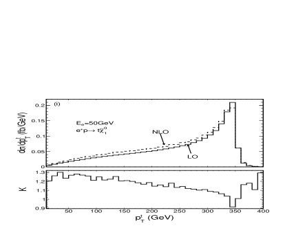
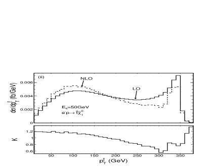
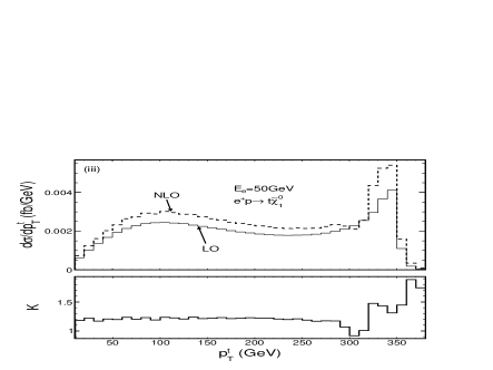
Figure 11: The LO, NLO QCD corrected distributions of the $p_{T}$ of final (anti-)top quark and the corresponding $K$-factors $\left(K(p_{T})\equiv\frac{d\sigma_{NLO}}{dp_{T}}/\frac{d\sigma_{LO}}{dp_{T}}\right)$ at the benchmark point at the $E_{e}=50~{}GeV$ and $E_{p}=7~{}TeV$ LHeC. (i) The process $e^{+}p\to t\tilde{\chi}^{0}_{1}+X$ in case (1). (ii) The process $e^{-}p\to\bar{t}\tilde{\chi}^{0}_{1}+X$ in case (1). (iii) The process $e^{+}p\to t\tilde{\chi}^{0}_{1}+X$ in case (2).

In Table 3, we present some typical numerical results with single dominance hypotheses of $\lambda_{131}^{\prime}=0.1$ [case (1)] and $\lambda_{132}^{\prime}=0.1$ [case (2)] for two electron beam energy configurations of $E_{e}=50~{}GeV$ and $E_{e}=150~{}GeV$ for comparison. With the assumption of integrated luminosities ${\cal L}_{int}=20~{}fb^{-1}$ and $2~{}fb^{-1}$ for $E_{e}=50~{}GeV$ and $E_{e}=150~{}GeV$, respectively, we can collect about $470$ and $220$ events for the $e^{+}p\to t\tilde{\chi}_{1}^{0}+X$ process in case (1) at the $E_{e}=50~{}GeV$ and $E_{e}=150~{}GeV$ LHeC, respectively. The corresponding relative statistic errors are estimated as $4.6\%$ and $6.7\%$, which are less than the QCD corrections of $11.5\%$ $(K=1.115)$ and $9.7\%$ $(K=1.097)$, respectively. Therefore, the QCD corrections might be resolvable for a precision measurement of $e^{+}p\to t\tilde{\chi}_{1}^{0}+X$ in case (1). However with the same luminosity assumptions, the LO and NLO corrected cross sections for the $e^{+}p\to t\tilde{\chi}^{0}_{1}+X$ process in case (2) at the $E_{e}=50~{}GeV$ LHeC are less than $1~{}fb$ and hardly resolvable in high precision measurement.

Process	$\sigma_{LO}$(fb)	$\sigma_{NLO}$(fb)	$K$-factor
$e^{+}p\to t\tilde{\chi}^{0}_{1}+X$ in Case (1)	101.91(1) $\parallel$ 21.240(3)	111.8(1) $\parallel$ 23.69(2)	1.097 $\parallel$ 1.115
$e^{-}p\to\bar{t}\tilde{\chi}^{0}_{1}+X$ in Case (1)	27.621(5) $\parallel$ 1.4101(3)	28.65(5) $\parallel$ 1.441(2)	1.037 $\parallel$ 1.022
$e^{+}p\to t\tilde{\chi}^{0}_{1}+X$ in Case (2)	13.820(2) $\parallel$ 0.7447(1)	14.85(2) $\parallel$ 0.998(1)	1.075 $\parallel$ 1.340

Table 3: The numerical results of the LO and NLO QCD corrected total cross sections for the processes $e^{+}p\to t\tilde{\chi}^{0}_{1}+X$, $e^{-}p\to\bar{t}\tilde{\chi}^{0}_{1}+X$ in case (1) and $e^{+}p\to t\tilde{\chi}^{0}_{1}+X$ in case (2) at the benchmark point at the $E_{e}=50~{}GeV$ and $E_{e}=150~{}GeV$ LHeC. The data on the left (right) side of the notation $\parallel$ correspond to the results at $E_{e}=150~{}GeV$ ($E_{e}=50~{}GeV$) LHeC.

4 Summary

In this paper, we calculate the NLO QCD corrections to the single (anti-)top quark production associated with a lightest neutralino in the MSSM with $R$-parity breaking coupling at the LHeC. In our calculations, we include completely all possible resonant and nonresonant diagrams and do not assume the production and decay factorization for the top squarks. The UV divergences are eliminated in the complex top squark mass scheme and the IR divergences are canceled by adopting both the TCPSS and DPS methods to make cross-check. The numerical calculations are carried out with the chosen SUSY parameters in the pMSSM-19, which is compatible with current experimental bounds. We investigate the dependence of the LO and the NLO QCD integrated cross sections on the top squark, neutralino, and gluino masses around the benchmark point. We also present the LO and the NLO QCD corrected distributions of the transverse momenta of final (anti-)top quark; they show that the impacts of the NLO QCD corrections might be resolvable in high precision measurement.

Acknowledgments: This work was supported in part by the National Natural Science Foundation of China (Grants No. 11075150, No. 11005101, No. 11275190), and the Fundamental Research Funds for the Central Universities (Grant No. WK2030040024).

References

- [1] ATLAS Collaboration, Report No. ATLAS-CONF-2013-007; ATLAS Collaboration, Report No. ATLAS-CONF-2013-024; ATLAS Collaboration, Phys. Lett. B 720 13 (2013); ATLAS Collaboration, J. High Energy Phys. 02 (2013) 0951.
- [2] CMS Collaboration, Report No. CMS PAS SUS-12-024; CMS Collaboration, Report No. CMS PAS SUS-13-007; CMS Collaboration, Phys. Rev. D 87 052006 (2013).
- [3] S. Kraml, arXiv:hep-ph/1206.6618.
- [4] Michele Papucci, Joshua T. Ruderman, and Andreas Weiler, Report No. DESY-11-193, CERN-PH-TH/265, J. High Energy Phys. 09 (2012) 035.
- [5] Junjie Cao, Zhaoxia Heng, Jin Min Yang, and Jingya Zhu, J. High Energy Phys. 10 (2012) 079; F. Mahmoudi, A. Arbey, M. Battaglia, and A. Djouadi, arXiv:hep-ph/1211.2794; Lorenzo Basso and Florian Staub, Phys. Rev. D 87 015011 (2013); Vernon Barger, Peisi Huang, Muneyuki Ishida, and Wai-Yee Keung, Phys. Rev. D 87 015003 (2013); Jiwei Ke, Hui Luo, Ming-Xing Luo et al., Phys. Lett. B 723 113 (2013); Zhaoxia Heng, arXiv:hep-ph/1210.3751; Marcela Carena, Stefania Gori, Ian Low et al., J. High Energy Phys. 02 (2013) 114.
- [6] Matthew W. Cahill-Rowley, et al., Eur. Phys. J. C 72 2156 (2012).
- [7] S. P. Martin, Phys. Rev. D 54, 2340 (1996); P. F. Pérez and S. Spinner, Phys. Lett. B 673, 251 (2009).
- [8] P. Fayte, Phys. Lett. B 69, 489 (1977).
- [9] G. R. Farrar, P. Fayte, Phys. Lett. B 76, 575 (1978).
- [10] S. Weinberg, Phys. Rev. D 26, 287 (1982).
- [11] N. Sakai and T. Yanagida, Nucl. Phys. B197, 533 (1982).
- [12] R. Barbier, C. Berat, M. Besancon et al., Phys. Rep. 420, 1 (2005).
- [13] L.E. Ibanez and G.G. Ross, Nucl. Phys. B368, 3 (1992).
- [14] J. L. Abelleira Fernandez et al., J. Phys. G 39 075001; J. L. Abelleira Fernandez, C. Adolphsen et al., arXiv:hep-ex/1211.5102; LHeC web page, http://www.lhec.org.uk.
- [15] T. Kon, T. Kobayashi, and S. Kitamura, Phys. Lett. B 333, 263 (1994); T. Kobayashi, S. Kitamura, and T. Kon, Int. J. Mod. Phys. A 11, 1875 (1996); T. Kon, T. Kobayashi, and S. Kitamura, Phys. Lett. B 376, 227 (1996); T. Kon, T. Kobayashi, Phys. Lett. B 409, 265 (1997).
- [16] H. Dreiner and P. Morawitz, Nucl. Phys. B503, 55 (1997).
- [17] Jihn E. Kim and P. Ko, Phys. Rev. D 57, 489 (1998).
- [18] J. Ellis, S. Lola, and K. Sridhar, Phys. Lett. B 408, 252 (1997).
- [19] Z. Kunszt, and W. J. Stirling, Z. Phys. C 75, 453 (1997).
- [20] Wei Hong-Tang, Zhang Ren-You, Guo Lei, Han Liang, Ma Wen-Gan et al., J. High Energy Phys. 07 (2011) 003.
- [21] M. Arai, K. Huitu, S.K. Rai, and K. Rao, J. High Energy Phys. 08 (2010) 082.
- [22] M.A. Bernhardt, H.K. Dreiner, S. Grab, and P. Richardson, Phys. Rev. D 78, 015016 (2008).
- [23] M. Chemtob and G. Moreau, Phys. Rev. D 61, 116004 (2000).
- [24] Siba Prasad Das, Amitava Datta, and Monoranjan Guchait, Phys. Rev. D 70, 015009 (2004).
- [25] R. Barbier et al., Phys. Rep. 420, 1 (2005).
- [26] F. Borzumati, and J.S. Lee, Phys. Rev. D 66, 115012 (2002).
- [27] A. Denner, S. Dittmaier, M. Roth, and L.H. Wieders, Nucl. Phys. B724, 247 (2005); A. Denner, S. Dittmaier, M. Roth, and D. Wackeroth, Nucl. Phys. B560, 33 (1999).
- [28] W. Beenakker, R. Höpker, and P. M. Zerwas, Phys. Lett. B378, 159 (1996); W. Beenakker, R. Höpker, T. Plehn, and P.M. Zerwas, Z. Phys. C 75, 349 (1997).
- [29] A. Denner, Fortschr. Phys. 41, 307 (1993).
- [30] W.J. Marciano, Phys. Rev. D 29, 580 (1984).
- [31] A. Denner and S. Dittmaier, Nucl. Phys. B844, 199 (2011).
- [32] G. t’Hooft and M. Veltman, Nucl. Phys. B153, 365 (1979); A. Denner, U. Nierste, and R. Scharf, Nucl. Phys. B367, 637 (1991); A. Denner and S. Dittmaier, Nucl. Phys. B658, 175 (2003).
- [33] P.F. Duan, R.Y. Zhang, W.G. Ma, L. Guo, and Y. Zhang, J. Phys. G 39, 105002 (2012).
- [34] H. K. Dreiner, S. Grab, M. Krämer, and M. K. Trenkel, Phys. Rev. D 75, 035003 (2007).
- [35] T. Kinoshita, J. Math. Phys. 3, 650 (1962).
- [36] T.D. Lee and M. Nauenberg, Phys. Rev. 133, B1549 (1964).
- [37] B.W. Harris and J.F. Owens, Phys. Rev. D 65, 094032 (2002).
- [38] Stefano Catani and Michael H. Seymour, Nucl. Phys. B485, 291 (1997).
- [39] J. Pumplin et al., J. High Energy Phys. 07 (2002) 012.
- [40] D. Stump et al., J. High Energy Phys. 10 (2003) 046.
- [41] C. Amsler et al., Phys. Lett. B 667, 1 (2008); K. Nakamura et al., J. Phys. G 37, 075021 (2010).
- [42] J. Beringer et al., Phys. Rev. D 86, 010001 (2012); http://pdglive.lbl.gov/listings1.brl?quickin=Y.1.
- [43] For recent papers, see, e.g. Manimala Chakraborty, Utpal Chattopadhyay, and Rohini M. Godbole, Phys. Rev. D 87, 035022 (2013); Howard Baer et al, Phys. Rev. D 87, 035017 (2013); Gautam Bhattacharyya and Tirtha Sankar Ray, Phys. Rev. D 87, 015017 (2013); Motoi Endo et al, Phys. Rev. D 85, 095006 (2012); E. Gabrielli, K. Kannike, B. Mele, A. Racioppi, and M. Raidal, Phys. Rev. D 86, 055014 (2012); Pran Nath, Int. J. Mod. Phys. A27 1230029 (2013).
- [44] Ernesto Arganda, J. Lorenzo Diaz-Cruz, Alejandro Szynkman, and Eur. Phys. J. C 73 2384 (2013); Wolfgang Altmannshofer, Marcela Carena et al., J. High Energy Phys. 01 (2013) 160; Stephen F. King, Margarete Muhlleitner et al., Nucl. Phys. B870 (2013).
- [45] For recent papers, see, e.g., F. Mahmoudi, A. Arbey, and M. Battaglia, arXiv:hep-ph/1211.2795; Alex Drlica-Wagner, arXiv:astro-ph.HE/1210.5558; D. P. Roy, arXiv:hep-ph/1211.3510; Leszek Roszkowski, Enrico Maria Sessolo, and Yue-Lin Sming Tsai, Phys.Rev. D 86 095005 (2012); C. Strege, et al, et al. J. Cosmol. Astropart. Phys. 03 (2012) 030.
- [46] For recent papers, see, e.g., F. Mahmoudi, and T. Hurth., arXiv:hep-ph/1211.2796; A. Arbey et al, Phys. Rev. D 87, 035026 (2013); Jonathan L. Feng, Konstantin T. Matchev, and David Sanford, Phys. Rev. D 85, 075007 (2012); A. Arbey and M. Battaglia, Eur. Phys. J. C 72 1906 (2012); M.W. Cahill-Rowley, J. L. Hewett, A. Ismail, and T. G. Rizzo, arXiv:1211.1981.
- [47] CMS Collaboration, Report No. CMS PAS Hig-13-005.
- [48] ATLAS Collaboration, Phys. Lett. B 716 1 (2012).
- [49] ATLAS Collaboration, Report No. ATLAS-CONF-2013-034.
- [50] ATLAS Collaboration, arXiv:1211.6956v2.
-
[51]
https://twiki.cern.ch/twiki/bin/view/AtlasPublic/CombinedSummaryPlotsSusyDirect
StopSummary. - [52] https://twiki.cern.ch/twiki/bin/view/CMSPublic/PhysicsResultsSUS.
- [53] B. C. Allanach, Comput. Phys. Commun. 143, 305 (2002).
- [54] A. Djouadi, M.M. Muhlleitner, and M. Spira, Acta Phys. Pol. B 38, 635 (2007).
- [55] R. Frederix, T. Gehrmann, and N. Greiner, J. High Energy Phys. 06 (2010) 086; R. Frederix, T. Gehrmann, and N. Greiner, J. High Energy Phys. 09 (2008) 122.
- [56] S. Catani, S. Dittmaier, M. H. Seymour, and Z. Trocsanyi, Nucl. Phys. B627, 189 (2002).