Bridging Information Criteria and Parameter Shrinkage
for Model Selection

Abstract

Model selection based on classical information criteria, such as BIC, is generally computationally demanding, but its properties are well studied. On the other hand, model selection based on parameter shrinkage by $\ell_{1}$-type penalties is computationally efficient. In this paper we make an attempt to combine their strengths, and propose a simple approach that penalizes the likelihood with data-dependent $\ell_{1}$ penalties as in adaptive Lasso and exploits a fixed penalization parameter. Even for finite samples, its model selection results approximately coincide with those based on information criteria; in particular, we show that in some special cases, this approach and the corresponding information criterion produce exactly the same model. One can also consider this approach as a way to directly determine the penalization parameter in adaptive Lasso to achieve information criteria-like model selection. As extensions, we apply this idea to complex models including Gaussian mixture model and mixture of factor analyzers, whose model selection is traditionally difficult to do; by adopting suitable penalties, we provide continuous approximators to the corresponding information criteria, which are easy to optimize and enable efficient model selection.

Keywords: Model selection, Parameter Shrinkage, Information criterion, Adaptive Lasso, Factor analysis, Gaussian mixture, Mixture of factor analysizers

1 Introduction

Model selection aims at choosing, from a set of candidates, a mathematical model that strikes a balance between simplicity and adequacy to the observed data. Traditionally, it is performed by optimizing some information criteria (ICs). In particular, the Bayesian information criterion (BIC, Schwarz (1978)), AIC (Akaike, 1973), and the minimum message length (MML) principle (Wallace and Freeman, 1987), are widely used in different statistical model selection problems. These criteria have a discrete feasible domain. Their optimization usually involves exhaustive search over all possible models, which is computationally intensive.

When the model is very complex or the space of candidate models is very large, a brute force testing of all possible models causes very high computational costs and becomes impractical. To tackle this problem, a lot of efforts have been made to adjust the model complexity continuously. For instance, for the linear regression problem, Lasso (Tibshirani, 1996) applies the $\ell_{1}$ penalty on the coefficients which could shrinking some coefficients to zero. Various approaches, including adaptive Lasso (ALasso, Zou (2006)), SCAD (Fan and Li, 2001), and FIRST (Hwang et al., 2009) make use of similar but different ways of parameter shrinkage. For finite mixture models, “entropic prior” (Brand, 1999) or the Dirichlet prior (Zivkovic and van der Heijden, 2004) for the mixing weights could produce sparsity of the mixing weights and hence perform model selection. However, in these methods, how to select the penalization parameter is usually a crucial issue. Moreover, asymptotic properties of these methods have been well studied, but less attention was paid to their performance on finite samples. It would be very useful if one can find their relationship to the IC-based approach for finite samples.

We aim to develop an efficient model selection approach which is based on the continuous penalized likelihood and approximately coincides with model selection based on ICs, such as BIC. We call this approach quick information criterion-like (Quick-IC) model selection. Our contributions are mainly two fold. First, for regular models, we establish a bridge between the penalized likelihood of ALasso and ICs, and propose to approximate the latter with the former, resulting in convenient model selection; this can also be considered as a way to directly determine the penalization parameter in ALasso to perform IC-like model selection, which avoids the search for the penalization parameter and would save a lot of computation, especially when iterative procedures are needed to find ALasso solutions. Specifically, in Sec. 2, we give the intuition that the penalty term for each parameter in ALasso is closely related to an indicator function showing if this parameter is active. Consequently, one can approximate the number of free parameters in ICs in terms of such penalty terms and find continuous approximators to the ICs. This inspires the proposed approach Quick-IC in Sec. 3, which is shown to select exactly the same model as the corresponding IC does in the case with a diagonal Fisher information matrix. General cases are also briefly discussed. The theoretical claims are verified by simulation studies in Section 4.

Second, in Sec. 5, we extend Quick-IC to non-regular and complex models, such as factor analysis, the Gaussian mixture model and the mixture of factor analyzers (Hinton et al., 1997), whose model selection is traditionally very difficult due to the large candidate model space. By making use of logarithm penalties with data-dependent weights, we provide continuous approximators to the ICs suitable for model selection of these models, and make their model selection easy and efficient. This illustrates the good applicability of the proposed approach.

2 Relating Adaptive Lasso to Information Criteria: Intuition

In this section we assume that the model under consideration satisfies some regularity conditions including identification conditions for the parameters $\boldsymbol{\theta}$, the consistency of the maximum likelihood estimate (MLE) $\hat{\boldsymbol{\theta}}$ when the sample size $n$ tends to infinity, and the asymptotic normality of $\hat{\boldsymbol{\theta}}$. The penalized likelihood can be written as

$$pl(\boldsymbol{\theta})=l(\boldsymbol{\theta})-\lambda p_{\lambda}(\boldsymbol{\theta}).$$ (1)

where $l(\boldsymbol{\theta})$ is the log-likelihood, $\boldsymbol{\theta}$ is the parameter vector, $p_{\lambda}(\boldsymbol{\theta})=\sum_{i}p_{\lambda}(\theta_{i})$ is the penalty, and $\lambda$ is the penalization parameter. The maximum penalized likelihood estimate is $\hat{\boldsymbol{\theta}}_{pl}=\arg\max\limits_{\boldsymbol{\theta}}pl(\boldsymbol{\theta})$.

$p_{\lambda}(\boldsymbol{\theta_{i}})=\sum_{i}|\theta_{i}|$ gives the $\ell_{1}$-norm penalty. The $\ell_{1}$ penalty produces sparse and continuous estimates (Tibshirani, 1996), and it has been shown to outperform other penalties in some scenarios (Ng, 2004). However, it also causes bias in the estimate of significant parameters, and it could select the true model consistently only when the data satisfy certain conditions (Zhao and Yu, 2006). Certain methods, including stability selection with the randomized Lasso (Meinshausen and Bühlmann, 2010) and ALasso (Zou, 2006), were proposed to overcome such disadvantages of the $\ell_{1}$ penalty.

In particular, ALasso uses $p_{\lambda}(\boldsymbol{\theta})=\sum_{i}\hat{w}_{i}|\theta_{i}|$, with $\hat{{w}}_{i}=1/|\hat{{\theta}}_{i}|^{\gamma}$, where $\gamma>0$, and $\hat{\boldsymbol{\theta}}$ is a (initial) MLE of $\boldsymbol{\theta}$. Consequently, the strength for penalizing different parameters depends on the magnitude of their estimate. Under some regularity conditions and the condition $\lambda_{n}/\sqrt{n}\rightarrow 0$ and $\lambda_{n}n^{(\gamma-1)/2}\rightarrow\infty$ (the subscript $n$ is used in $\lambda_{n}$ to indicate the dependence of $\lambda$ on the sample size $n$), the ALasso estimator is consistent in model selection. We are more interested in its behavior on finite samples.

The result of ALasso depends on the penalization parameter $\lambda$. For very simple models, one may use least angle regression (LARS, Efron et al. (2004)) to compute the entire solution path, which gives all possible solutions as $\lambda$ changes. Among these solutions, the best model can then be selected by cross-validation or based on some ICs (Zou et al., 2007). (The latter approach is compared with our approach in Sec. 4, and one can see that it may give very different results from the corresponding IC.) However, for complex models, especially when iterative algorithms are used to find the solution corresponding to a given $\lambda$, it is computationally very demanding and impractical to find the solution path. One then needs to select the penalization parameter in advance. In the next section we show that one can simply determine this parameter, while the model selection result approximately coincides with that based on ICs.

Let us focus on the case $\gamma=1$, meaning that

$$p_{\lambda}(\theta_{i})=\hat{w}_{i}|\theta_{i}|=|\theta_{i}|/|\hat{\theta}_{i}|.$$ (2)

After the convergence of the ALasso procedure, insignificant parameters become zero, and $p_{\lambda}(\theta_{i})=0$ for such parameters. On the other hand, with suitable $\lambda_{n}$, the ALasso estimator $\hat{\theta}_{i,AL}$ is also consistent (Zou, 2006); roughly speaking, significant parameters are then expected to be changed little by the penalty, when $n$ is not very small. Consequently, at convergence, $p_{\lambda}(\theta_{i})=|\hat{\theta}_{i,AL}|/|\hat{\theta}_{i}|\approx 1$ for significant parameters. That is, the penalty $p_{\lambda}(\theta_{i})$ approximately indicates whether the parameter $\theta_{i}$ is active or not. Suppose that the parameters are not redundant. $\sum_{i}p_{\lambda}(\theta_{i})$ is then an approximator of the number of active parameters, denoted by $D$, in the resulting model.

Recall that the traditional ICs whose minimization enables model selection can be written as

$$\textrm{IC}_{D}=-l(\hat{\boldsymbol{\theta}}_{D})+\lambda_{IC}D.$$ (3)

The BIC and AIC criteria are obtained by setting the value of $\lambda_{IC}$ to

$$\lambda_{BIC}=1/2\cdot\log n,\textrm{~{}~{}and~{}~{}}\lambda_{AIC}=1,$$ (4)

respectively. Relating (3) to the penalized likelihood (1), one can see that in ALasso, by setting $\lambda=\lambda_{IC}$ ($\lambda_{IC}$ may be $\lambda_{BIC}$, $\lambda_{AIC}$, etc.), the maximum penalized likelihood is closely related to the IC (3). This will be rigorously studied next, and in fact $\lambda=2\lambda_{IC}$ (instead of $\lambda=\lambda_{IC}$) gives interesting results.

3 Basic Approach for Quick-IC Model Selection

3.1 With a Diagonal Fisher Information Matrix

Can we make the model selection results of ALasso exactly the same as those based on the ICs? In fact, if the Fisher information matrix is diagonal, this can be achieved by simply setting $\lambda$ in ALasso to $2\lambda_{IC}$, i.e., maximizing the following penalized likelihood

$$pl(\boldsymbol{\theta})=l(\boldsymbol{\theta})-2\lambda_{IC}\sum_{i}|\theta_{i}|/|\hat{\theta}_{i}|$$ (5)

selects the same model as the IC (3) does, as seen from the following proposition.

Proposition 1

Suppose that the following conditions hold. 1. The log-likelihood $l(\boldsymbol{\theta})$ is quadratic around the MLE $\hat{\boldsymbol{\theta}}$, with a non-singular observed Fisher information matrix $\hat{\mathbf{I}}(\hat{\boldsymbol{\theta}})$. 2. $\hat{\mathbf{I}}(\hat{\boldsymbol{\theta}})$ is diagonal. Then the non-zero parameters selected by maximizing (5) are exactly those selected by minimizing the IC (3).

Proof Since the MLE $\hat{\boldsymbol{\theta}}$ maximizes $l(\boldsymbol{\theta})$, we have $\frac{\partial l(\boldsymbol{\theta})}{\partial\boldsymbol{\theta}}\Big{|}_{\boldsymbol{\theta}=\hat{\boldsymbol{\theta}}}=\mathbf{0}$. Let $\mathbf{H}\triangleq n\hat{\mathbf{I}}(\hat{\boldsymbol{\theta}})$. Under the assumptions made in the proposition, the log-likelihood becomes

$$l(\boldsymbol{\theta})=l(\hat{\boldsymbol{\theta}})-\frac{1}{2}(\boldsymbol{\theta}-\hat{\boldsymbol{\theta}})^{T}\mathbf{H}(\boldsymbol{\theta}-\hat{\boldsymbol{\theta}})=l(\hat{\boldsymbol{\theta}})-\frac{1}{2}\sum_{i}\mathbf{H}_{ii}({\theta}_{i}-\hat{{\theta}}_{i})^{2}.$$ (6)

The penalized likelihood (5) then becomes

$$pl(\boldsymbol{\theta}) = l(\boldsymbol{\theta})-2\lambda_{IC}\sum_{i}(|\theta_{i}|/|\hat{\theta}_{i}|)$$

$$= l(\hat{\boldsymbol{\theta}})-\frac{1}{2}\sum_{i}\mathbf{H}_{ii}(\theta_{i}-\hat{\theta}_{i})^{2}-2\lambda_{IC}\sum_{i}(|\theta_{i}|/|\hat{\theta}_{i}|).$$

It is easy to show that the solutions maximizing $pl(\boldsymbol{\theta})$ are

$$\hat{\theta}_{i,AL}=\textrm{sgn}(\hat{\theta}_{i})\cdot\big{(}|\hat{\theta}_{i}|-2\lambda_{IC}/(\mathbf{H}_{ii}\cdot|\hat{\theta}_{i}|)\big{)}^{+}.$$

That is, $\hat{\theta}_{i,AL}$ estimated by maximizing (5) is non-zero if and only if $|\hat{\theta}_{i}|-2\lambda_{IC}\cdot/(\mathbf{H}_{ii}\cdot|\hat{\theta}_{i}|)>0$, i.e.,

$$\mathbf{H}_{ii}\cdot\hat{\theta}_{i}^{2}>2\lambda_{IC}.$$ (7)

On the other hand, the model selected by minimizing the criterion (3) has $D^{*}$ free parameters if $IC_{D^{*}}<IC_{{D^{*}}-1}$ and $IC_{D^{*}}\leq IC_{{D^{*}}+1}$. According to (3), we then have

$$l(\hat{\boldsymbol{\theta}}_{{D^{*}}+1})-l(\hat{\boldsymbol{\theta}}_{{D^{*}}})\leq\lambda_{IC},~{}\textrm{and~{}}l(\hat{\boldsymbol{\theta}}_{D^{*}})-l(\hat{\boldsymbol{\theta}}_{D^{*}-1})>\lambda_{IC}.$$ (8)

The least change in $l(\boldsymbol{\theta})$ caused by eliminating a particular parameter has been derived in the optimal brain surgeon (OBS) technique (Hassibi and Stork, 1993). Here, due to the simple form of (6), the least change in $l(\boldsymbol{\theta})$ caused by eliminating $\theta_{i}$, denoted by $S_{i}$, can be seen directly:

$$S_{i}=\frac{1}{2}\hat{\theta}_{i}^{2}/[\mathbf{H}^{-1}]_{ii}=\frac{1}{2}[\mathbf{H}]_{ii}\cdot\hat{\theta}_{i}^{2}.$$ (9)

Note that $l(\hat{\boldsymbol{\theta}}_{D^{*}})-l(\hat{\boldsymbol{\theta}}_{D^{*}-1})$ in (8) is the minimum of $S_{i}$ for all $D^{*}$ parameters in the current model. Therefore, one can see that model selection based on the IC (3) selects $\theta_{i}$ if and only if $S_{i}>\lambda_{IC}$, which is equivalent to the constraint (7). That is, under the assumptions made in the proposition, non-zero parameters produced by maximizing the penalized likelihood (5) are exactly those selected by the corresponding IC (3). $\blacksquare$  

This proposition indicates that (5) can be considered as a continuous approximator to the ICs (3), which enables Quick-IC; one can see that the continuous approximator is obtained by simply replacing the maximum likelihood $l(\hat{\boldsymbol{\theta}}_{D})$ by the data likelihood $l(\boldsymbol{\theta})$, and replacing the number of free parameters, $D$, by $2\sum_{i}|\theta_{i}|/|\hat{\theta}_{i}|$.

3.2 More General Case

The condition in Proposition 1 is rather restrictive; in the linear regression scenario, it corresponds to the orthogonal design case. In the more general case, where $\hat{\mathbf{I}}(\hat{\boldsymbol{\theta}})$ is usually not diagonal, the condition for the parameters $\theta_{i}$ to be selected by maximizing (5) becomes more complex, and (3) and (5) are usually not exactly equivalent. We give some results on the relationship between Quick-IC and model selection based on ICs.

Proposition 2

Suppose that condition 1 in Proposition 1 holds. Assume that both the IC approach (3) and Quick-IC (5) perform model selection in the backword elimination manner, i.e., the penalization parameter is gradually increased to the target value, such that insignificant parameters are set to zero one by one. Further assume that once a parameter is set to zero, it will not become non-zero again. Let $\widetilde{\mathbf{H}}\triangleq\textrm{diag}(\hat{\boldsymbol{\theta}})\cdot\mathbf{H}\cdot\textrm{diag}(\hat{\boldsymbol{\theta}})$, where $\mathbf{H}=n\hat{\mathbf{I}}(\boldsymbol{\theta})$ and is assumed to be nonsingular. Then the IC approach (3) selects $\theta_{i}$ if and only if $[\widetilde{\mathbf{H}}^{-1}]_{ii}<\frac{1}{2\lambda_{IC}}$, while Quick-IC (5) does so if and only if $[\widetilde{\mathbf{H}}^{-1}]_{i\cdot}\mathbb{I}<\frac{1}{2\lambda_{IC}}$, where $[\widetilde{\mathbf{H}}^{-1}]_{i\cdot}$ donotes the $i$th row of $\widetilde{\mathbf{H}}^{-1}$ and $\mathbb{I}$ is the vector of 1’s.

Proof  From the proof of Proposition 1 or Hassibi and Stork (1993), one can see that the IC approach selects $\theta_{i}$ if and only if $S_{i}=\frac{1}{2}\hat{\theta}_{i}^{2}/{[\mathbf{H}^{-1}]_{ii}}>\lambda_{IC}$, which is equivalent to $[\widetilde{\mathbf{H}}^{-1}]_{ii}<\frac{1}{2\lambda_{IC}}$. Let $\tilde{{\theta}}_{i}\triangleq{{\theta}}_{i}/\hat{{\theta}}_{i}$. On the other hand, due to Condition 1 in Proposition 1, the penalized likelihood with the penalization parameter $\lambda$ is

$$J = l(\boldsymbol{\theta})-\lambda\sum_{i}|\theta_{i}|/|\hat{\theta}_{i}|$$

$$= l(\hat{\boldsymbol{\theta}})-\frac{1}{2}(\boldsymbol{\theta}-\hat{\boldsymbol{\theta}})^{T}\mathbf{H}(\boldsymbol{\theta}-\hat{\boldsymbol{\theta}})-\lambda\sum_{i}|\theta_{i}|/|\hat{\theta}_{i}|$$

$$= l(\hat{\boldsymbol{\theta}})-\frac{1}{2}(\tilde{\boldsymbol{\theta}}-\mathbb{I})^{T}\widetilde{\mathbf{H}}(\tilde{\boldsymbol{\theta}}-\mathbb{I})-\lambda\sum_{i}\tilde{\theta}_{i}.$$

Clearly, if $\lambda$ is very small such that none of $\theta_{i}$ is set to zero, $J$ is maximized when $\frac{\partial J}{\partial\tilde{\boldsymbol{\theta}}}=\mathbf{0}$, i.e.,

$$\widetilde{\mathbf{H}}(\mathbb{I}-\tilde{\boldsymbol{\theta}})-\lambda\mathbb{I}=\mathbf{0},$$

which is equivalent to $\mathbb{I}-\tilde{\boldsymbol{\theta}}=\lambda\widetilde{\mathbf{H}}^{-1}\mathbb{I}$. Consequently, we have

$$\tilde{\theta}_{i}=1-\lambda[\widetilde{\mathbf{H}}^{-1}]_{i\cdot}\mathbb{I}.$$

When $\lambda$ is gradually increased such that $\lambda[\widetilde{\mathbf{H}}^{-1}]_{j.}\mathbb{I}=1$, $\tilde{\theta}_{j}$, or equivalently ${\theta}_{j}$, is set to zero. Finally, when $\lambda$ is increased to $2\lambda_{IC}$, the non-zero parameters $\theta_{i}$ selected by Quick-IC satisfy $[\widetilde{\mathbf{H}}^{-1}]_{i\cdot}\mathbb{I}<\frac{1}{2\lambda_{IC}}$. $\blacksquare$  

Although in practice one may not adopt backword elimination, the above proposition helps us understand the similarity and difference between the IC approach and Quick-IC. For example, if $\sum_{j\neq i}[{\mathbf{H}}^{-1}]_{ij}=0$ for all $i$ (which includes Proposition 1 as a special case), the two approaches give the same results. Of course, for finite samples, in the general case it is theoretically impossible to make parameter shrinkage-based Quick-IC exactly identical to the IC approach. However, their empirical comparisons in various situations presented in Sec. 4 suggest that they usually give the same model selection results for various sample sizes.

We give the following remarks on the proposed model selection approach. Firstly, the result of the proposed approach depends on $\hat{\boldsymbol{\theta}}$. When the model is very large, $\hat{\boldsymbol{\theta}}$ may be too rough, and it is useful to update $\hat{\boldsymbol{\theta}}$ using a consistent estimator sometime when a smaller model is derived. Secondly, in Sec. 5 the idea of Quick-IC is further applied to more complex models, by using data-dependent weights for suitable penalization functions and approximating the number of effective parameters. For example, in some cases one needs to resort to the logarithm penalty to produce sparsity of parameters, and we suggest using the corresponding data-adaptive penalty $\hat{w}_{i}\log(\frac{|\theta_{i}|+\epsilon}{\epsilon})$ with $\hat{w}_{i}=1/\log(\frac{|\hat{\theta}_{i}|+\epsilon}{\epsilon})$, where $\epsilon$ is a very small positive number, as the penalty term, as discussed in Section 5.3. Correspondingly, to obtain the continuous approximator of the ICs, one just simply replaces the number of effective parameters in $\theta_{i}$ with $2\sum_{i}\hat{w}_{i}\log(\frac{|\theta_{i}|+\epsilon}{\epsilon})$.

4 Numerical Studies

The proposed approach in Section 3 directly applies to model selection of simple models such as regression and vector auto-regression (VAR). VAR provides a convenient way for Granger causality analysis (Granger, 1980), and has a lot of applications in economics, neuroscience, etc. Unfortunately it usually involves quite a large number of parameters, making the IC approach impractical, while Quick-IC gives efficient model selection.

In this section we use simulations to investigate the performance of Quick-IC. To verify the results in Sec. 3, we consider the simple linear regression problem $y=\boldsymbol{\theta}^{T}\mathbf{x}+\epsilon$, where $y$ is the target, $\mathbf{x}=(x_{1},...,x_{p})^{T}$ contains predictors, and $\epsilon$ is the Gaussian noise. We take BIC as an example, i.e., we compare BIC-like Quick-IC (or Quick-BIC, with $\lambda_{IC}=\lambda_{BIC}$ in (5)) with the original BIC (3). We also compare them with the approach of ALasso followed by the BIC criterion (ALasso+BIC): one first finds the solution path of ALasso using LARS, and then selects the “best” model by evaluating the BIC criterion with the maximum likelihood $l(\hat{\boldsymbol{\theta}}_{D})$ replaced by the likelihood of the parameter values on the solution path (Zou et al. (2007), Sec. 4). For this reason, ALasso+BIC is different from BIC. In Quick-BIC, the noise variance was estimated from the full model. For BIC, we searched the prediction number between 4 and 8.

20 predictors $x_{i}$ were used, i.e., $p=20$. 14 entries of $\boldsymbol{\theta}$ were set to zero. The magnitudes of the others were randomly chosen between 0.2 and 2.5, and the signs were arbitrary. We considered three cases. Case I corresponded to an orthogonal design, i.e., all predictors are uncorrelated. In Case II, the pairwise correlation between $x_{i}$ and $x_{j}$ was set to be $0.5^{|i-j|}$. In the last case, the covariance matrix of $\mathbf{x}$ was randomly generated as $\mathbf{M}\mathbf{M}^{T}$ with entries of the square matrix $\mathbf{M}$ randomly sampled between $-0.5$ and $0.5$. In all cases we normalized the variance of each $x_{i}$. The noise variance was $0.5$. To see the sample size effect, we varied the sample size $n$ from 100 to 300. The simulation was repeated for 100 random trials.

Table 1 reports the frequency of the differences in the selected predictor numbers given by different methods. One can see that in Case I, all the three methods almost always select the same number of predictors. In Cases II and III, Quick-BIC still gives rather similar results to BIC; in particular, as the sample size increases, their results tend to agree with each other quickly. ALasso+BIC produces different models with a surprisingly noteworthy chance for both sample sizes, especially in Case III. However, it seems to be still statistically consistent in model selection, like BIC; we found that when $n=600$, for 56 times it gave the same model as BIC. As for the computational loads, BIC took more than 550 times longer than Quick-BIC as well as ALasso+BIC.

Table 1: Occurrence frequency of the differences in the numbers of selected predictors by different methods for 100 random trials. “$<$” and “$>$” mean “$<-1$” and “$>1$”, respectively; $D_{BIC}^{*}$, $D_{Quick-BIC}^{*}$, and $D_{ALasso+BIC}^{*}$ denote the numbers of predictors produced by BIC, Quick-BIC, and ALasso+BIC, respectively.

Case	$T$	$D_{BIC}^{*}-D_{Quick-BIC}^{*}$					$D_{BIC}^{*}-D_{ALasso+BIC}^{*}$					$D_{Quick-BIC}^{*}-D_{ALasso+BIC}^{*}$
		-2	-1	0	1	2	$<$	-1	0	1	$>$	$<$	-1	0	1	$>$
I	100	0	4	96	0	0	0	3	97	0	0	0	0	99	1	0
	300	0	1	99	0	0	0	0	100	0	0	0	0	99	1	0
II	100	1	5	92	2	0	2	3	73	15	7	2	1	74	16	7
	300	0	0	100	0	0	0	0	89	11	0	0	0	89	11	0
III	100	3	12	67	14	4	20	29	33	13	5	21	26	37	11	5
	300	0	6	87	7	0	27	29	42	2	0	27	32	38	3	0

5 Extensions: Quick-IC by Approximating Various Information Criteria

Below we focus on other frequently-used statistical models, especially some complex ones, and give continuous approximators to the ICs for their model selection by extending Quick-IC. We also give empirical results to illustrate the applicability and efficiency of Quick-IC.

5.1 General Framework with Grouped Parameters

For regular statistical models, under a set of regularity conditions, the asymptotic normality of $\hat{\boldsymbol{\theta}}$ holds. The $\ell_{1}$ penalty used in Lasso can then produce sparsity of the parameters and hence perform model selection Tibshirani (1996). The asymptotic properties of the variable selection techniques established in the linear regression scenario also approximately hold for regular models. For some non-regular models, it is still possible to do so. If the gradient of the log-likelihood changes slowly around $\hat{\boldsymbol{\theta}}$, these penalties will successfully push insignificant parameters to zero. Otherwise, one may apply penalization on suitable transformations of the parameters, instead of the original parameters.

In practice, the parameters in a model often naturally belong to groups, i.e., they are selected or discarded simultaneously (Yuan and Lin, 2006; Bach, 2008). One can formalize this by introducing functions $\mathcal{T}_{i}$ which allow computation of the penalties for groups of variables. Generally speaking, the information criterion of the form (3) can be approximated by the negative penalized likelihood:

$$npl(\boldsymbol{\theta})=-l(\boldsymbol{\theta})+2\lambda_{IC}\cdot\sum_{i}D_{fi}\cdot p_{\lambda}(\mathcal{T}_{i}(\boldsymbol{\theta})),$$ (10)

where $\mathcal{T}_{i}(\boldsymbol{\theta})$ are suitable transformations of the parameters (or selected parameters) controlling the complexity of the model, and $D_{fi}$ are the numbers of independent parameters associated with the group $\mathcal{T}_{i}(\boldsymbol{\theta})$. Minimization of the negative penalized likelihood (10) enables simultaneous model selection and parameter estimation. When a particular $\mathcal{T}_{i}(\boldsymbol{\theta})$ is pushed to zero, $D_{fi}$ free parameters disappear, and the model complexity is reduced. How to choose $\mathcal{T}_{i}(\boldsymbol{\theta})$ and to calculate $D_{fi}$ depends on the specific model.

5.2 Quick BIC-Like Model Selection for Factor Analysis

Let us first consider model selection of the factor analysis (FA) model. In FA, the observed $d$-dimensional data vector $\mathbf{x}=(x_{1},\cdots,x_{d})^{T}$ is modeled as $\mathbf{x}=\mathbf{Ay}+\mathbf{e}$, where $\mathbf{A}$ is the factor loading matrix, $\mathbf{y}=(y_{1},\cdots,y_{k})^{T}$ the vector of $k$ underlying Gaussian factors, and $\mathbf{e}=(e_{1},\cdots,e_{d})^{T}$ the vector of uncorrelated Gaussian errors with the covariance matrix $\boldsymbol{\Psi}=\textrm{diag}(\psi_{1},\cdots,\psi_{d})$. The factors $\mathbf{y}$ and the errors $\mathbf{e}$ are also mutually independent. Here, we have assumed that $\mathbf{x}$ is zero-mean and that the factors $\mathbf{y}$ are normally distributed with zero mean and identity covariance matrix.

Given the factor number $k$ and a set of observations $\{\mathbf{x}_{t}\}_{t=1}^{n}$, the FA model can be fitted by maximum likelihood (ML) using the expectation-maximization (EM) algorithm (Rubin and Thayer, 1982; Ghahramani and Hinton, 1997). But ML estimation could not determine the optimal factor number $k^{*}$, since the ML does not consider the complexity of the model and it increases as $k$ grows.

A suitable factor number gives the FA model enough capacity and avoids over-fitting. When the unconditional variances of $y_{i}$ are fixed, model selection of FA can be achieved by shrinking suitable columns of $\mathbf{A}$ to zero. So entries in each column of $\mathbf{A}$ are grouped. Denote by $\mathbf{A}_{(i)}$ the $i$th column of $\mathbf{A}$. Note that $||\mathbf{A}_{(i)}||$ is singular at $\mathbf{A}_{(i)}=\mathbf{0}$, so penalization on $||\mathbf{A}_{(i)}||$ can remove unnecessary columns in $\mathbf{A}$ and consequently perform model selection. The negative penalized likelihood for approximating BIC is

$$npl^{FA}=-l^{FA}+2D_{f}\cdot\lambda_{BIC}\sum_{i=1}^{k}p_{\lambda}(||\mathbf{A}_{(i)}||),$$ (11)

where $D_{f}$ denotes the number of free parameters in the column of $\mathbf{A}$ which is to be removed, and $\lambda_{BIC}$ is given in (4). Due to the rotation indeterminacies of the factors $y_{i}$, the total number of free parameters in $\mathbf{A}$ is $dk-\frac{k(k-1)}{2}$. The proposed method removes columns of $\mathbf{A}$ one by one. If one insignificant column of $\mathbf{A}$ is shrinked to zero, the total number of free parameters in $\mathbf{A}$ reduces from $dk-\frac{k(k-1)}{2}$ to $d(k-1)-\frac{(k-1)(k-2)}{2}$. Therefore, $D_{f}$ can be evaluated to equal $d-k+1$, as the change of the number of free parameters in $\mathbf{A}$ when a certain column disappears. Once a column of $\mathbf{A}$ is removed, $k$ is updated accordingly.

The EM algorithm for minimizing the negative penalized likelihood (11) can be derived analogously to the derivation of that for the FA model (Ghahramani and Hinton, 1997). Following Fan and Li (2001), we use the local quadratic approximation (LQA) to approximate the penalties $p_{\lambda}(||\mathbf{A}_{(i)}||)$. As a great advantage, it admits a closed-form solution for $\mathbf{A}$ in the M step.

We would like to address the following advantages of adopting the negative penalized likelihood based on ALasso, instead of the original BIC criterion, for model selection. 1. The negative penalized likelihood is easy to minimize. 2. If the log-likelihood function is concave in the neighborhood of the maximum likelihood estimator (like in the linear regression problem), the negative penalized likelihood is convex, and its minimization does not suffer from multiple local minima.

5.3 Quick MML-Like Model Selection for Gaussian Mixture Model

The Gaussian mixture model (GMM) models the density of the $d$-dimensional variable $\mathbf{x}$ as a weighted sum of some Gaussian densities: $f(\mathbf{x})=\sum_{i=1}^{m}\pi_{i}\phi(\mathbf{x};\boldsymbol{\mu}_{i},\boldsymbol{\Sigma}_{i})$, where $\phi(\mathbf{x};\boldsymbol{\mu}_{i},\boldsymbol{\Sigma}_{i})$ are Gaussian densities with mean $\boldsymbol{\mu}_{i}$ and covariance matrix $\boldsymbol{\Sigma}_{i}$, and $\pi_{i}$ are nonnegative weights that sum to one.

BIC is not suitable for model selection of mixture models, since not all data are effective for estimating the parameters specifying an individual component. Instead, the MML-based model selection criterion is preferred (Figueiredo and Jain, 2002). The message length to be minimized for model selection of GMM is

$$\mathcal{L}^{GM}_{MML}=\frac{D_{f}^{GM}}{2}\sum_{i:\pi_{i}>0}\log\Big{(}\frac{n\pi_{i}}{12}\Big{)}+\frac{m_{nz}}{2}\log\Big{(}\frac{n}{12}\Big{)}+\frac{m_{nz}(D_{f}^{GM}+1)}{2}-l^{GM},$$ (12)

where $m_{nz}$ denotes the number of non-zero-probability components, and the number of free parameters in each component is $D_{f}^{GM}=d+d(d+1)/2=d^{2}/2+3d/2$. Minimization of the above function is troublesome since it involves the discrete variable $m_{nz}$. Below we develop an approximator to (12) which is continuous in $\pi_{i}$.

GMM is a typical non-regular statistical model. The expected complete-data log likelihood of GMM (see McLachlan and Peel (2000) for its formulation), which gives an approximation of the true data likelihood, involves $\log\pi_{i}$. Hence, its gradient w.r.t. $\pi_{i}$ grows very fast when $\pi_{i}\rightarrow 0$. Consequently, the $\ell_{1}$ penalty could not push insignificant $\pi_{i}$ to zero. Fortunately, one can then naturally exploit the $\log$ penalty to produce sparsity of $\pi_{i}$. The $\log$ penalty on $\pi_{i}$ also has the advantage of admitting a closed-form update equation for $\pi_{i}$ in the EM algorithm. To avoid the discontinuity of the objective function when a component with $\pi_{i}\rightarrow 0$ vanishes, we use $\log(\frac{\varepsilon+\pi_{i}}{\varepsilon})=\log(\varepsilon+\pi_{i})-\log(\varepsilon)$ as the penalty, where $\varepsilon$ is a small enough positive number (we chose $10^{-3}$ in experiments). Let $\hat{w}_{i}\triangleq 1/\log[(\varepsilon+\hat{\pi}_{i})/\varepsilon]$. Inspired by the idea of adaptive weights in ALasso, we can let the penalty term be $\hat{w}_{i}\log[(\pi_{i}+\epsilon)/\epsilon]$. $m_{nz}$ could then be approximately by 2$\sum_{i=1}^{m}\hat{w}_{i}{\log[(\varepsilon+\pi_{i})/\varepsilon]}$. Consequently, (12) is approximated by

$$npl^{GM}_{MML}=\frac{D_{f}^{GM}}{2}\sum_{i:\pi_{i}>0}\log\Big{(}\frac{n\pi_{i}}{12}\Big{)}+\Big{[}\log\Big{(}\frac{n}{12}\Big{)}+D_{f}^{GM}+1\Big{]}\sum_{i=1}^{m}\hat{w}_{i}\log\Big{(}\frac{\pi_{i}+\epsilon}{\epsilon}\Big{)}-l^{GM}.$$ (13)

The EM algorithm for minimizing the function above is the same as that for maximizing the GMM likelihood, except that the update equation for $\pi_{i}$ is changed to

$$\pi_{i}=\max\Big{\{}0,\frac{\sum_{t=1}^{n}h_{it}-0.5D_{f}^{GM}-0.5\hat{w}_{i}[\log(n/12)+D_{f}^{GM}+1]}{n-0.5mD_{f}^{GM}-0.5[\log(n/12)+D_{f}^{GM}+1]\sum_{j=1}^{m}\hat{w}_{j}}\Big{\}},$$

where $h_{it}$ denotes the posterior probability that the $t$th point comes from the $i$th component. When $\pi_{i}$ becomes very small, say smaller than $1/n$, we drop the $i$-th component. In practice, if the initialized model is very far from the desired one, as the model complexity reduces, it is better to occasionally update $\hat{w}_{i}$ with the corresponding maximum likelihood estimator.

5.4 Quick MML-Like Model Selection for Mixture of Factor Analyzers

Now consider the mixture of factor analyzers (MFA, Hinton et al. (1997)), which has a lot of applications in pattern recognition. It assumes that the $d$-dimensional observations $\mathbf{x}$ can be modeled as $\mathbf{x}=\boldsymbol{\mu}_{i}+\mathbf{A}_{i}\mathbf{y}_{i}+\mathbf{e}_{i}\textrm{~{}with probability~{}}\pi_{i}\textrm{~{}}(i=1,\cdots,m)$, where $\boldsymbol{\mu}_{i}$ is the mean of the $i$th factor analyzer, and local factors $\mathbf{y}_{i}$, which follow $\mathcal{N}(\mathbf{0},\mathbf{I}_{k_{i}})$, are independent from $\mathbf{e}_{i}$, which follow $\mathcal{N}(\mathbf{0},\boldsymbol{\Psi})$ with $\boldsymbol{\Psi}=\textrm{diag}(\psi_{i},\cdots,\psi_{d})$. The factor number $k_{i}$ may vary for different $i$.

Following Figueiredo and Jain (2002), one can find the message length for MFA (with some constant terms dropped):

$$\mathcal{L}^{MFA}_{MML} = \frac{1}{2}\sum_{i:\pi_{i}>0}\Big{[}D_{fi}^{F}\cdot\log\Big{(}\frac{n\pi_{i}}{12}\Big{)}\Big{]}+\frac{1}{2}\sum_{i=1}^{m_{nz}}D_{fi}^{F}+\frac{m_{nz}}{2}\Big{[}\log\Big{(}\frac{n}{12}\Big{)}+1\Big{]}-l^{MFA},$$ (14)

where $D_{fi}^{F}$ denotes the number of free parameters specifying the $i$-th factor analyzer, i.e., $D_{fi}^{F}=d+dk_{i}-k_{i}(k_{i}-1)/2$. This function involves integers $m_{nz}$ (the number of factor analyzers) and $k_{i}$, $i=1,\cdots,m_{nz}$, (the number of factors in each factor analyzer). Its optimization is computationally highly demanding due to the large search space of $(m_{nz},{k_{i}}_{i=1}^{m_{nz}})$. Using the $\ell_{1}$ and $\log$ penalties with data-adaptive weights, we can approximate $\mathcal{L}^{MFA}_{MML}$ with the following function:

$$npl_{MML}^{MFA} = \frac{1}{2}\sum_{i:\pi_{i}>0}\hat{D}_{fi}^{F}\log\Big{(}\frac{n\pi_{i}}{12}\Big{)}+\sum_{i=1}^{m}\hat{w}_{i}\log\Big{(}\frac{\pi_{i}+\epsilon}{\epsilon}\Big{)}$$ (15)

$$\cdot\Big{[}\hat{D}_{fi}^{F}+\log\Big{(}\frac{n}{12}\Big{)}+1\Big{]}-l^{MFA},$$

where $\hat{D}_{fi}^{F}=\hat{N}_{f}(\mathbf{A}_{i})+d$ and $\hat{N}_{f}(\mathbf{A}_{i})$ is the ALasso-based approximator to the number of free parameters in $\mathbf{A}_{i}$. After some derivations, one can see that a reasonable approximator is $\hat{N}_{f}(\mathbf{A}_{i})=\big{[}dk_{i}-\frac{k_{i}(k_{i}-1)}{2}\big{]}-D_{f}\sum_{j=1}^{k_{i}}\Big{(}1-p_{\lambda}(||\mathbf{A}_{i,(j)}||)\Big{)}=\frac{k_{i}(k_{i}-1)}{2}+(d-k_{i}+1)\sum_{j=1}^{k_{i}}p_{\lambda}(||\mathbf{A}_{i,(j)}||)$. One can verify that $\hat{N}_{f}(\mathbf{A}_{i})$ changes very slightly when $k_{i}$ is reduced by shrinking columns of $\mathbf{A}_{i}$. Similar to Ghahramani and Hinton (1997), one can derive the EM algorithm for minimizing (15).

We note that the proposed model selection methods for GMM and MFA generate new components or split any large component. For very complex problems, they may converge to local optima. If necessary, one can perform the split and merge operations (Ueda et al., 1999) after certain EM iterations to improve the final results.

5.5 Experiments

5.5.1 Factor Analysis

We generated the data according to the FA model, and compared four model selection schemes, which are BIC-like Quick-IC given in Section 5.2 (or Quick-BIC), BIC, AIC, and fivefold cross-validation (CV). The true factor number was $k=5$, and the data dimension was $d=10$. Elements in $\mathbf{A}$ were randomly generated between $-1.5$ and $1.5$, and the error variances $\psi_{i}$ were random numbers between 0 and 1. When using BIC, AIC, or CV, we let $k_{min}=3$ and $k_{max}=7$, while Quick-BIC was initialized with 8 factors. To investigate the sample size effect, we let the sample size $n$ be 40 and $100$. In each case, we repeated all methods for 100 random trials.

When $n=40$, BIC, AIC, Quick-BIC, and CV approximately took 4, 4, 1.5, and 20 seconds, respectively, for each trial. Clearly Quick-BIC is most computationally appealing, as expected. Fig. 1 plots the histogram of the factor numbers found by the four methods. When $n=40$, BIC (as well as Quick-BIC) seems to over-penalize the model complexity and results in a smaller factor number. But when $n$ is increased to 100, its performance becomes almost the best. On the contrary, AIC seems to under-penalize the complexity. In both cases, Quick-BIC is always similar to BIC. Also considering its light computational load, Quick-BIC is preferred among the four methods. We also tested the case $n=200$, and found that Quick-BIC and BIC give clearly the best results.

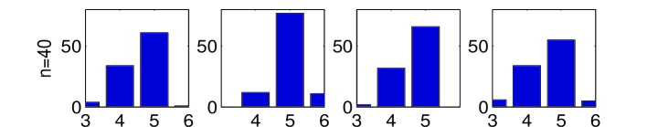
(a) BIC          (b) AIC        (c) Quick-BIC     (d) CV   

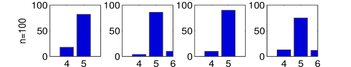
     (e) BIC          (f) AIC        (g) Quick-BIC     (h) CV   

Figure 1: Occurrence frequency for various $k$ (100 trials). The true value is 5. Top/bottom: $n$=40/100.

5.5.2 Gaussian Mixture Model

We compared the approach Quick-IC which minimizes the continuous version of MML (13) with the MML-based method proposed in Figueiredo and Jain (2002) (denoted by FJ’s method), in terms of the chances of finding the preferred component number and the CPU time.

Here we present the results on two data sets. For each data set, we repeated each method for 100 trials. In each trial, the data were randomly generated, and for initialization, the mean of each Gaussian component was randomly chosen from the data points. The results on the “shrinking spiral” data set (Ueda et al., 1999) are given in Fig. 2(a-c), and Fig. 2(d-f) shows the results on the “triangle data”, which were obtained by rotating and shifting three sets of bivariate Gaussian points following $\mathcal{N}(\mathbf{0},\textrm{diag}(2.25,0.25))$. For the first data set, we set $m_{max}=30$ for both methods and $m_{min}=3$ for FJ’s method. The CPU time taken by Quick-IC and FJ’s method was $4$ and $33$ seconds, respectively. For the second data set, we let $m_{max}=20$ and $m_{min}=1$ for FJ’s method. The CPU time was about $7$ and $21$ seconds for the two methods. Fig. 2(b, e) and (c, f) give the histograms of the component numbers obtained by FJ’s method and Quick-IC. One can see that they give similar results. However, FJ’ method seems to produce less robust (more disperse) results for the spiral data. We conjecture that it is caused by the “annihilation” process in FJ’s method (Figueiredo and Jain, 2002): FJ’s method annihilates the least probable component (with the smallest mixing weight $\hat{\pi}_{i}$) to obtain a smaller model. This process is discontinuous, and simply uses the magnitude of the mixing weight to indicate the significance of the corresponding component. In fact the significance of a particular component also depends on its relationship to other components. As a consequence, when a component that has the least weight but is actually significant is removed, the message length $\mathcal{L}^{GM}_{MML}$ may increase, resulting in a sub-optimal model .

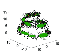
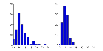
(a) spiral data              (b) FJ’s          (c) Quick-IC       

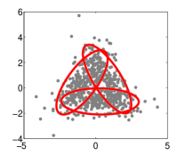
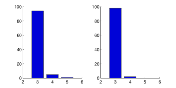
   (d) triangle data            (e) FJ’s          (f) Quick-IC       

Figure 2: Experimental result on GMM learning. (a-c) spiral data with 900 points. (d-f) triangle data with 600 points. (a, d) data points and typical results. (b, e) histograms of the number of components learned by FJ’s method for 100 trials. (c, f) histograms of the number of components learned by Quick-IC.

5.5.3 Mixture of Factor Analyzers

Quick-IC uses the MML approximator (15) to determine both the number of factor analyzers ($m$) and the local factor numbers ($k_{i}$) in the MFA model. We tested the spiral data (Figure 2a), and repeated the experiments with 50 trials. $m$ was initialized as $30$ and all of $k_{i}$ were initialized as $3$. The number of factor analyzers learned by our approach is always between 10 and 13 (with the chances 10: 8/50, 11: 21/50, 12: 14/50, and 13: 7/50). In the resulting model, most factor analyzers have 1 factor, and occasionally there is one factor analyzer with 2 factors (with one dominating the other) or with no factor. This is consistent with the previous results with $k_{i}$ a prior set to 1 (Figueiredo and Jain, 2002).

We then constructed another synthetic data set in which the local factor number varies for different factor analyzers. Fig. 3(a) plots the data points without noise, and (b) shows the observed noisy data. The sample size was 5390. Quick-IC was compared with the variational Bayesian method (VBMFA, Ghahramani and Beal (2000)). We repeated both methods for 20 trials with different initializations. Quick-IC and VBMFA took about $1.5$ and $10$ minutes for each run, and produced $9\sim 13$ and $10\sim 14$ factor analyzers, respectively. Note that the data are clearly non-Gaussian, so some factor analyzers may overlap to some extent to model the data well. Fig. 3(c) and (d) show the results of the two method in one run. Since Quick-IC does not generate new local factor analyzers, it cannot separate two factor analyzers which are initialized together. This can be alleviated by using a large $m$ for initialization. On the other hand, sometimes VBMFA may split one factor analyzer into two; we found that in 2 trials VBMFA divided the “arm” or “leg” into two segments.

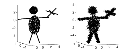
(a)                             (b)                       

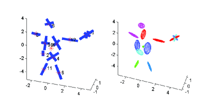
                         (c)                             (d)                       

Figure 3: Results of MFA with factor analyzers having different $k_{i}$. (a) noiseless points. (b) noisy data for analysis. (c) a structure learned by Quick-IC, with $m=12$. (d) that by VBMFA, with $m=12$. Note that (c) plots columns of loading matrices, while (d) depicts the contour of the Gaussian distribution of each factor analyzer.

6 Conclusion and Future Work

We showed that under some conditions, the penalty used in adaptive Lasso, which is the $\ell_{1}$ penalty with a data-dependent weight, resembles an indicator function showing if this parameter is active. This motivated us to approximate the traditional model selection criterion by the penalized likelihood with a fixed penalization parameter. The latter is continuous in the parameters, greatly facilitating the model selection procedure. We formulated this idea as the Quick-IC approach. We showed that for finite samples, Quick-IC produces exactly the same model as the corresponding information criterion when the Fisher information matrix is diagonal. We also investigated more general cases. Furthermore, for some complex and non-regular models, we provided continuous approximators to their model selection criteria, by using suitable penalty forms and data-adaptive weights. We have demonstrated that for these models, our simple approach is computationally very efficient in model selection, and that its results are similar to those produced by the corresponding IC. One line of our future research is to investigate the theoretical properties of Quick-IC for non-regular models such as finite mixture models.

References

- Akaike (1973) H. Akaike. Information theory and an extension of the maximum likelihood principle. Proc. 2nd International Symposium on Information Theory, pages 267–281, 1973.
- Bach (2008) F. Bach. Consistency of the group lasso and multiple kernel learning. Journal of Machine Learning Research, 9:1179–1225, 2008.
- Brand (1999) M.E. Brand. Structure learning in conditional probability models via an entropic prior and parameter extinction. Neural Computation, 11(5):1155–1182, 1999.
- Candás et al. (2008) E. Candás, M. Wakin, and S. Boyd. Enhancing sparsity by reweighted minimization. The Journal of Fourier Analysis and Applications, 14:877–905, 2008.
- Chen and Chen (2008) J. Chen and Z. Chen. Extended bayesian information criteria for model selection with large model spaces. Biometrika, 95:759–771, 2008.
- Draper (1995) D. Draper. Assessment and propagation of model uncertainty. J. Roy. Stat. Soc.: Ser. B (Methodol.), 57:45–97, 1995.
- Efron et al. (2004) B. Efron, T. Hastie, I. Johnstone, and R. Tibshirani. Least angle regression. The Annals of Statistics, 32:407–499, 2004.
- Fan and Li (2001) J. Fan and R. Li. Variable selection via nonconcave penalized likelihood and its oracle properties. J. Amer. Statist. Assoc., 96:1348–1360, 2001.
- Figueiredo and Jain (2002) M.A.T. Figueiredo and A.K. Jain. Unsupervised learning of finite mixture models. IEEE Transactions on Pattern Analysis and Machine Intelligence, 24(3):381–396, 2002.
- Ghahramani and Beal (2000) Z. Ghahramani and M. Beal. Variational inference for Bayesian mixtures of factor analysers. In Advances in Neural Information Processing Systems 12, pages 449–455, Cambridge, MA, 2000. MIT Press.
- Ghahramani and Hinton (1997) Z. Ghahramani and G.E. Hinton. The EM algorithm for mixtures of factor analyzers. Technical Report CRG-TR-96-1, Department of Computer Science, University of Toronto, Toronto, Canada, 1997.
- Granger (1980) C. Granger. Testing for causality: A personal viewpoint. Journal of Economic Dynamics and Control, 2:329–352, 1980.
- Hassibi and Stork (1993) B. Hassibi and D. G. Stork. Second order derivatives for network pruning: Optimal brain surgeon. In Advances in Neural Information Processing Systems 5, pages 164–171. Morgan Kaufmann, 1993.
- Hinton et al. (1997) G.E. Hinton, P. Dayan, and M. Revow. Modeling the manifolds of images of handwritten digits. IEEE transactions on Neural Networks, 8:65–74, 1997.
- Hwang et al. (2009) W.Y. Hwang, H.H. Zhang, and S. Ghosal. First: Combining forward iterative selection and shrinkage in high dimensional sparse linear regression. Statistics and Its Interface, 2:341–348, 2009.
- McLachlan and Peel (2000) G. McLachlan and D. Peel. Finite Mixture Models. John Wiley and Sons, 2000.
- Meinshausen and Bühlmann (2010) N. Meinshausen and Bühlmann. Stability selection. Journal of the Royal Statistical Society: Series B, 72:417–473, 2010.
- Ng (2004) A.Y. Ng. vs. regularization, and rotational invariance. In Proceedings of the 21st International Conference on Machine Learning, pages 78–85, New York, NY, USA, 2004.
- Rubin and Thayer (1982) D. Rubin and D. Thayer. EM algorithms for ml factor analysis. Psychometrika, 47(1):69–76, 1982.
- Schwarz (1978) G. Schwarz. Estimating the dimension of a model. The Annals of Statistics, 6:461C464, 1978.
- Tibshirani (1996) R. Tibshirani. Regression shrinkage and selection via the lasso. Journal of the Royal Statistical Society, B., 58(1):267–288, 1996.
- Ueda et al. (1999) N. Ueda, R. Nakano, Z. Ghahramani, and G.E. Hinton. SMEM algorithm for mixture models. In Advances in Neural Information Processing Systems 11, pages 599–605, Cambridge, MA, 1999. MIT Press.
- Wallace and Freeman (1987) C.S. Wallace and P.R. Freeman. Estimation and inference by compact coding. J. Roy. Stat. Soc.: Ser. B (Methodol.), 49:240–265, 1987.
- Yuan and Lin (2006) M. Yuan and Y. Lin. Model selection and estimation in regression with grouped variables. Journal of the Royal Statistical Society, Series B, 68(1):49–67, 2006.
- Zhao and Yu (2006) P. Zhao and B. Yu. On model selection consistency of lasso. Journal of Machine Learning Research, 7:2541–2563, 2006.
- Zivkovic and van der Heijden (2004) Z. Zivkovic and F. van der Heijden. Recursive unsupervised learning of finite mixture models. IEEE Transactions on Pattern Analysis and Machine Intelligence, 26(5):651–265, 2004.
- Zou (2006) H. Zou. The adaptive lasso and its oracle properties. Journal of the American Statistical Association, 101(476):1417–1429, 2006.
- Zou et al. (2007) H. Zou, T. Hastie, and R. Tibshirani. On the “degrees of freedom” of the lasso. The Annals of Statistics, 35:2173–2192, 2007.