Compression of unitary rank–structured matrices to CMV-like shape with an application to polynomial rootfinding

Abstract

This paper is concerned with the reduction of a unitary matrix $U$ to CMV-like shape. A Lanczos–type algorithm is presented which carries out the reduction by computing the block tridiagonal form of the Hermitian part of $U$, i.e., of the matrix $U+U^{H}$. By elaborating on the Lanczos approach we also propose an alternative algorithm using elementary matrices which is numerically stable. If $U$ is rank–structured then the same property holds for its Hermitian part and, therefore, the block tridiagonalization process can be performed using the rank–structured matrix technology with reduced complexity. Our interest in the CMV-like reduction is motivated by the unitary and almost unitary eigenvalue problem. In this respect, finally, we discuss the application of the CMV-like reduction for the design of fast companion eigensolvers based on the customary QR iteration.

Keywords CMV matrices, unitary matrices, rank–structured matrices, block tridiagonal reduction, QR iteration, block Lanczos algorithm, complexity MSC 65F15

1 Introduction

In a recent paper [14], Killip and Nenciu conduct a systematic study of the properties of a class of unitary matrices –named CMV matrices from the names of the researchers who introduced the class in [6]–. The rationale of the paper emphasized in the title is that CMV matrices are the unitary analogue of Hermitian tridiagonal Jacobi matrices. It is interesting to consider potential analogies from the point of view of numerical computations since the Hermitian tridiagonal structure provides a very efficient and compressed representation of Hermitian matrices especially for eigenvalue computation. To our knowledge the first fundamental contribution along this line was provided in the paper [5] where some algorithms are presented for the reduction of a unitary matrix to a CMV-like form and, moreover, the properties of this form under the QR process are investigated. In [16] a more general framework is proposed, which includes the CMV-like form as a particular instance.

Our interest in the CMV reduction of unitary matrices stems from the research of numerically efficient eigenvalue algorithms for unitary and almost unitary rank–structured matrices. The structural properties of the classical Hessenberg reduction of a unitary matrix were extensively exploited for fast eigenvalue computation in some pioneering papers by Gragg and coauthors [1, 17, 18]. More recently, it has been realized that these properties are related with the rank structures of a Hessenberg unitary matrix and, moreover, these structures are invariant under the QR iteration thus yielding a large variety of possible fast adaptations of this iterative method for eigenvalue computation of unitary and almost unitary matrices [2, 3, 8]. A common issue of all these approaches is that rank–structured matrices are generally represented in a data–sparse format and the accurate update of this format under the iterative process can be logically complicated and time consuming. Additionally, these difficulties are magnified for block matrices where the size of the condensed representation typically increases. So the point of view taken in this paper is that, for numerical and computational efficiency of eigensolvers, it would be better to replace the data-sparse format with a sparser representation employing directly the matrix entries. The CMV reduction naturally lead to a sparser form.

This paper is aimed to explore the mechanism underlying the reduction of a general unitary matrix $U\in\mathbb{C}^{n\times n}$ into some CMV-like form. It is shown that an origin of such mechanism can be found in the property that under some mild assumption the matrices $U_{H}\colon=U+U^{H}$ and $U_{AH}\colon=U-U^{H}$ can be simultaneously reduced into block tridiagonal form by a unitary congruence, i.e., $U_{H}\rightarrow T_{H}=Q^{H}U_{H}Q$ and $U_{AH}\rightarrow T_{AH}=Q^{H}U_{AH}Q$. From this it follows that the same transformation acts on the matrix $U$ by performing the reduction into block tridiagonal form, that is, $U\rightarrow\displaystyle\frac{T_{H}+T_{AH}}{2}=Q^{H}UQ$. A careful look at the out-of-diagonal blocks of $\displaystyle\frac{T_{H}+T_{AH}}{2}$ reveals that these are of rank one at most by showing the desired CMV-like shape of the matrix. The complexity of the block tridiagonal reduction is generally $O(n^{3})$. However there are some interesting structures which can be exploited. In particular, if $U$ is rank-structured then $U+U^{H}$ is also rank-structured and Hermitian so that the fast techniques developed in [11] might be incorporated in the algorithm by achieving a quadratic complexity.

The paper is organized as follows. In Section 2, we describe and analyze a block Lanczos procedure for the reduction of $U_{H}$ and simultaneously of $U_{AH}$ into block tridiagonal form. It is also shown that this procedure is at the core of our CMV–ification algorithm for unitary matrices. In Section 3 by elaborating on the Lanczos approach we propose a different CMV reduction algorithm in Householder style using elementary matrices and comment on the cost analysis of the algorithm in the case of rank–structured inputs. In Section 4 we discuss the application of the CMV-like representation of a unitary matrix in the design of fast eigensolvers for unitary and almost unitary matrices. Finally, in Section 5 the conclusion and further developments are drawn.

2 Derivation of the Algorithm

Let $U\in\mathbb{C}^{n\times n}$ denote a unitary matrix. In this section we consider the problem of reducing $U$ into a sparse form referred to as CMV–like shape.

Definition 1.

We say that an $n\times n$ unitary matrix $U$ has CMV-like shape or, for short, is a CMV-like matrix if it is block tridiagonal, that is,

$$U=\left[\begin{array}[]{ccccc}U_{1}&\tilde{U}_{1}\\ \hat{U}_{1}&\ddots&\ddots\\ &\ddots&\ddots&\tilde{U}_{p-1}\\ &&\hat{U}_{p-1}&U_{p}\end{array}\right],$$

where $U_{k}\in\mathbb{C}^{i_{k}\times i_{k}}$, $1\leq k\leq p$, $i_{1}=\ldots=i_{p-1}=2$ and $i_{p}\in\{1,2\}$ depending on the parity of $n$, and, moreover, both the superdiagonal and the subdiagonal blocks are matrices of rank one at most.

In the generic case a CMV–like matrix $U$ can be converted into a matrix with the CMV–shape described in Definition 1.2 in [14] by means of a unitary diagonal congruence. However, our class is a bit more general since it includes the direct sum of CMV shaped matrices together with some more specific matrices. For instance, the $4\times 4$ unitary matrix $U$ given by

$$U=\left[\begin{array}[]{cccc}0&1&0&0\\ \cos{\theta}&0&0&\sin{\theta}\\ -\sin{\theta}&0&0&\cos{\theta}\\ 0&0&1&0\end{array}\right],\quad(\theta\in\mathbb{R}),$$

is not CMV shaped according to the definition in [14] but it is CMV-like and it can be reduced into a pure CMV shape by a unitary congruence.

In order to investigate the reduction of a unitary matrix $U$ into CMV–like shape let us introduce the Hermitian and the anti-hermitian part of $U$ defined by $U_{H}\colon=\displaystyle\frac{U+U^{H}}{2}$ and $U_{AH}=\displaystyle\frac{U-U^{H}}{2}$ , respectively. If $U$ has at least three distinct eigenvalues then the minimal polyanalytic polynomial $p(z)$ of $U$ is $p(z)=z\bar{z}-1$, that is, $p(z)$ is the minimal (w.r.t. a fixed order) degree polynomial in $z$ and $\bar{z}$ such that $p(U)=0$. Observe that

$$z\bar{z}-1=\frac{(z+\bar{z})z}{2}-\frac{(z-\bar{z})z}{2}-1.$$ (1)

A block variant of the customary Lanczos method can be used to compute a block tridiagonal reduction of the Hermitian matrix $U_{H}$. The process is defined by the choice of the initial approximating subspace $\mathcal{D}_{0}=<\mathbf{z},\mathbf{w}>$. A simple version of the algorithm is given below.

Procedure Block_Lanczos Input: $U_{H}$, $D_{0}=[\mathbf{z}|\mathbf{w}]$; $[G,R,V]={\bf svd}(D_{0})$; $s={\bf rank}(R)$; $Q(:,1:s)=G(:,1:s)$; $s0=1,s1=s$; while $s1<n$ $W=U_{H}\cdot Q(:,s0:s1)$; $T(s0:s1,s0:s1)=(Q(:,s0:s1))^{H}\cdot U_{H}\cdot Q(:,s0:s1)$; if $s0=1$     $W=W-Q(:,s0:s1)\cdot T(s0:s1,s0:s1)$; else     $W=W-Q(:,s0:s1)\cdot T(s0:s1,s0:s1)$;     $W=W-Q(:,\hat{s}0:\hat{s}1)\cdot T(\hat{s}0:\hat{s}1,s0:s1);$ end $[G,R,V]={\bf svd}(W)$; $snew={\bf rank}(R)$; if $snew=0$     disp(’premature stop’); return; else     $R=R(1:snew,1:snew)\cdot(V(:,1:s))^{H}$;     $\hat{s}0=s0,\hat{s}1=s1,s0=s1+1,s1=s1+snew$;     $Q(:,s0:s1)=G(:,1:snew)$, $T(s0:s1,\hat{s}0:\hat{s}1)=R(1:snew,1:s)$;     $T(\hat{s}0:\hat{s}1,s0:s1)=(T(s0:s1,\hat{s}0:\hat{s}1))^{H}$, $s=snew$; end end $T(s0:s1,s0:s1)=(Q(:,s0:s1))^{H}*U_{H}*Q(:,s0:s1)$;

If the procedure Block_Lanczos terminates without premature stop then at the very end the unitary matrix $Q$ transforms $U_{H}$ into the Hermitian block tridiagonal matrix $T_{H}=Q^{H}\cdot U_{H}\cdot Q$, where

$$T_{H}=\left[\begin{array}[]{cccc}A_{1}&B_{1}^{H}\\ B_{1}&A_{2}&\ddots\\ &\ddots&\ddots&B_{p-1}^{H}\\ &&B_{p-1}&A_{p}\end{array}\right],$$

with $A_{k}\in\mathbb{C}^{i_{k}\times i_{k}}$, $B_{k}\in\mathbb{C}^{i_{k+1}\times i_{k}}$, and $2\geq i_{k}\geq i_{k+1}$, $i_{1}+\ldots=i_{p}=n$. The sequence $\{i_{k}\}_{k=0}^{p}$ ($i_{0}=1$) is formed from the values attained by the variable $s$ in the procedure Block_Lanczos.

Observe that from $Q\cdot T_{H}=U_{H}\cdot Q$ it follows inductively that for the subspaces

$$\begin{array}[]{ll}\mathcal{B}_{j}(U_{H},Q(:,1:i_{1}))=\mbox{\rm{block--span}}\{Q(:,1:i_{1}),U_{H}\cdot Q(:,1:i_{1}),\ldots,U_{H}^{j-1}\cdot Q(:,1:i_{1})\}\\ \colon=\{\sum_{k=0}^{j-1}U_{H}^{k}Q(:,1:i_{1})\Psi_{k},\ \Psi_{k}\in\mathbb{C}^{i_{1}\times i_{1}}\}\end{array}$$

and

$$\begin{array}[]{ll}\mathcal{Q}_{j}=\mbox{\rm{block--span}}\{Q(:,1:i_{1}),Q(:,i_{1}+1:i_{1}+i_{2}),\ldots,Q(:,\sum_{k=1}^{j-1}i_{k}+1:\sum_{k=1}^{j}i_{k})\}\\ \colon=\{\sum_{k=0}^{j-1}Q(:,\sum_{\ell=0}^{k}i_{\ell}+1:\sum_{\ell=0}^{k+1}i_{\ell})\Phi_{k},\ \Phi_{k}\in\mathbb{C}^{i_{k+1}\times i_{1}}\}\end{array}$$

it holds

$$\mathcal{B}_{j}(U_{H},Q(:,1:i_{1}))\subseteq\mathcal{Q}_{j},\quad j\geq 1.$$

Moreover, since

$$U_{H}^{j-1}\cdot Q(:,1:i_{1})=Q(:,\sum_{k=1}^{j-1}i_{k}+1:\sum_{k=1}^{j}i_{k})B_{j-1}\cdots B_{1}+\sum_{\ell=1}^{j-2}Q(:,\sum_{k=1}^{\ell-1}i_{k}+1:\sum_{k=1}^{\ell}i_{k})\Gamma_{\ell},$$ (2)

and $B_{k-1}\cdots B_{1}\in\mathbb{C}^{i_{k}\times i_{1}}$ is of maximal rank $i_{k}$ since the blocks $B_{i}$ are obtained with the Block_Lanczos procedure. Then we obtain

$$\mathcal{B}_{j}(U_{H},Q(:,1:i_{1}))=\mathcal{Q}_{j},\quad j\geq 1.$$

Conversely, this relation implies that the matrix $Q^{H}\cdot U_{H}\cdot Q$ is block upper Hessenberg and therefore block-tridiagonal.

Now let us consider the matrix $H\colon=Q^{H}\cdot U_{AH}\cdot Q$. We are going to investigate the structure of this matrix under the additional assumption that $\mathbf{w}=U\mathbf{z}$. Differently speaking, we suppose that the initial approximating subspace $\mbox{\rm{block--span}}\{Q(:,1:i_{1})\}$ satisfies $\mbox{\rm{block--span}}\{Q(:,1:i_{1})\}=\mbox{\rm{block--span}}\{D_{0}\}$, with $D_{0}=\left[\mathbf{z},U\mathbf{z}\right]$ depending on just one vector.

In the following lemma we prove that if the Block_Lanczos procedure does not occur in a breakdown, the size of the blocks $A_{k}$ and $B_{k}$ is $2$, with the exception of the last block in the case $n$ is odd.

Lemma 1.

Let us consider the algorithm Block_Lanczos applied to $U_{H}$ with the initial vectors $D_{0}=[\mathbf{z}|U\mathbf{z}]$, $\mathbf{z}\in\mathbb{C}^{n}$ and assume that the set of vectors, for $j\geq 1$, $U_{H}^{j-1}\mathbf{z},U_{H}^{j-1}U\mathbf{z}$ yields a basis of the whole space $\mathbb{C}^{n}$. Then the unitary matrix $Q$ satisfies (7) with $i_{1}=\ldots=i_{p-1}=2$ and $i_{p}\in\{1,2\}$ depending on the parity of $n$.

Proof.

The proof of the lemma consists in proving that the matrices $W$ generated in the procedure Block_Lanczos have always rank $2$, except for the last block in the case $n$ is odd.

Assume by contradiction that at step $j$, $j<n/2$ for $n$ even, $j<n/2-1$ for $n$ odd, we have a matrix $W$ such that $\mbox{\rm{rank }}(W)<2$, and that in previous steps all the corresponding matrices $W$ had full rank. The first $2j$ columns of the unitary matrix $Q$ returned by the procedure Block_Lanczos, form an orthogonal basis for the space $\mathcal{B}_{j}(U_{H},Q(:,1:i_{1}))$. Since $U$ is unitary it is easy to see that $\mathcal{B}_{j}(U_{H},Q(:,1:i_{1}))=\mbox{span}\{\mathbf{z},U\mathbf{z}|U^{H}\mathbf{z},U^{2}\mathbf{z}|\ldots,|(U^{H})^{j-1}\mathbf{z},U^{j}\mathbf{z}\}$. Since $\mbox{\rm{rank }}(W)<2$ then a nonzero linear combination of $(U^{H})^{j-1}z$ and $U^{j}z$ must be in $\mathcal{B}_{j-1}(U_{H},Q(:,1:i_{1}))$. Due to the unitariness of $U$, this means that both $(U^{H})^{j}\mathbf{z}$ and $U^{j+1}\mathbf{z}$ are in $\mathcal{B}_{j}(U_{H},Q(:,1:i_{1}))$. So the dimension of $\mathcal{B}_{j+1}(U_{H},Q(:,1:i_{1}))$ is $2j$ and this implies that $\mbox{\rm{rank }}(W)=0$, i.e. a premature termination, which is a contradiction. ∎

Theorem 2.

Let us consider the algorithm Block_Lanczos applied to $U_{H}$ with the initial vectors $D_{0}=[\mathbf{z}|U\mathbf{z}]$, $\mathbf{z}\in\mathbb{C}^{n}$. Let us assume that the set of vectors $U_{H}^{j-1}\mathbf{z},U_{H}^{j-1}U\mathbf{z}$, $j\geq 1$, yields a basis of the whole space $\mathbb{C}^{n}$, or, equivalently, the algorithm does not return an early termination warning. Then the unitary matrix $Q\in\mathbb{C}^{n\times n}$ reduces simultaneously $U_{H}$ and $U_{AH}$ into a block triangular form, that is,

$$T_{H}\colon=Q^{H}U_{H}Q=\left[\begin{array}[]{cccc}A_{1}&B_{1}^{H}\\ B_{1}&A_{2}&\ddots\\ &\ddots&\ddots&B_{p-1}^{H}\\ &&B_{p-1}&A_{p}\end{array}\right],$$

and

$$T_{AH}\colon=Q^{H}U_{AH}Q=\left[\begin{array}[]{cccc}A_{1}^{\prime}&-B_{1}^{\prime H}\\ B_{1}^{\prime}&A_{2}^{\prime}&\ddots\\ &\ddots&\ddots&-B_{p-1}^{\prime H}\\ &&B_{p-1}^{\prime}&A_{p}^{\prime}\end{array}\right]$$

where $A_{k},A_{k}^{\prime}\in\mathbb{C}^{2\times 2}$, $B_{k},B_{k}^{\prime}\in\mathbb{C}^{2\times 2}$, and in the case $n$ is odd, $A_{p}\in\mathbb{C}^{1\times 1}$, $B_{p-1},B_{p-1}^{\prime}\in\mathbb{C}^{1\times 2}$.

Proof.

In order to compare the shape of $H=Q^{H}\,\cdot\,U_{AH}\,\cdot\,Q$ and $T_{H}$ we first introduce a commensurable partitioning of $H$, i.e., $H=(H_{k,\ell}),H_{k,\ell}\in\mathbb{C}^{2\times 2}$, (possibly for odd $n$, $H_{p,\ell}\mathbb{C}^{1\times 2}$, and $H_{p,p}\in\mathbb{C}$). Clearly, we have that

$$\mathcal{B}_{j}(U_{AH},Q(:,1:i_{1}))=\mathcal{B}_{j}(U_{AH},D_{0}),\quad j\geq 1.$$

Let us begin by considering the initial step $j=1$. We have

$$U_{AH}\mathbf{z}=-U_{H}\mathbf{z}+U\mathbf{z}\in\mbox{\rm{block--span}}\{Q(:,1:i_{1}),Q(:,i_{1}+1:i_{1}+i_{2})\}.$$ (3)

Concerning $U_{AH}U\mathbf{z}$ from (1) we obtain that

$$U_{AH}U\mathbf{z}=U_{H}U\mathbf{z}-\mathbf{z}\in\mbox{\rm{block--span}}\{Q(:,1:i_{1}),Q(:,i_{1}+1:i_{1}+i_{2})\}.$$ (4)

By using (3) and (4) it is found that

$$U_{AH}Q(:,1:i_{1})=U_{H}Q(:,1:i_{1})\Delta+Q(:,1:i_{1})\Gamma,$$ (5)

for suitable matrices $\Delta,\Gamma\in\mathbb{C}^{i_{1}\times i_{1}}$ with $\Delta$ of maximal rank $i_{1}$. Since $U_{AH}$ and $U_{H}$ commute, from (2) and (5) by induction it follows that

$$\mathcal{B}_{j}(U_{AH},Q(:,1:i_{1}))\subseteq\mathcal{Q}_{j},\quad j\geq 1,$$

and

$$U_{AH}^{j-1}\cdot Q(:,1:i_{1})=Q(:,\sum_{k=1}^{j-1}i_{k}+1:\sum_{k=1}^{j}i_{k})B_{j-1}\cdots B_{1}\Delta^{j-1}+\sum_{\ell=1}^{j-2}Q(:,\sum_{k=1}^{\ell-1}i_{k}+1:\sum_{k=1}^{\ell}i_{k})\Gamma^{\prime}_{\ell},$$ (6)

for suitable matrices $\Gamma_{\ell}$, which says that

$$\mathcal{B}_{j}(U_{AH},Q(:,1:i_{1}))=\mathcal{Q}_{j},\quad j\geq 1,$$

and, therefore, the matrix $H$ is block upper Hessenberg, i.e., $H_{k,\ell}=0$ for $k-1>\ell$. On the other hand, since $U_{AH}$ is anti-hermitian we find that also $H$ is anti-hermitian and, hence, $H$ is block tridiagonal with the same shape as $T_{H}$. Finally, this implies that both $Q^{H}\cdot U\cdot Q$ and $Q^{H}\cdot U^{H}\cdot Q$ are in block tridiagonal form with the same shape as $H$ and $T_{H}$. ∎

From this result it follows that the unitary transformation induced by the matrix $Q$ has the same action when performed on the unitary matrix $U=\displaystyle\frac{U_{H}+U_{AH}}{2}\in\mathbb{C}^{n\times n}$. i.e,

$$T\colon=Q^{H}UQ=\left[\begin{array}[]{cccc}\hat{A}_{1}&\tilde{B}_{1}^{H}\\ \hat{B}_{1}&\hat{A}_{2}&\ddots\\ &\ddots&\ddots&\tilde{B}_{p-1}^{H}\\ &&\hat{B}_{p-1}&\hat{A}_{p}\end{array}\right]$$ (7)

where $\hat{A}_{k}\in\mathbb{C}^{2\times 2}$, $\hat{B}_{k}=\frac{B_{k}+B_{k}^{\prime}}{2}\in\mathbb{C}^{2\times 2},\tilde{B}_{k}^{H}=\frac{B_{k}^{H}-B_{k}^{\prime H}}{2}\in\mathbb{C}^{2\times 2}$, for $k=1,\ldots,\lfloor n/2\rfloor$, and in the case $n$ is odd, $\hat{A}_{p}\in\mathbb{C},\hat{B}_{p-1},\tilde{B}_{p-1}\in\mathbb{C}^{1\times 2}$. As proved in Lemma 1, blocks $B_{k}$ of $T_{H}$ are $2\times 2$ and have full rank.

In next step of our investigation on the shape of the matrix $T$ we give a careful look at the rank of its out-of-diagonal blocks.

Corollary 1.

Let us consider the algorithm Block_Lanczos applied to $U_{H}$ with the initial vectors $D_{0}=[\mathbf{z}|U\mathbf{z}]$, $\mathbf{z}\in\mathbb{C}^{n}$ and assume that the set of vectors $U_{H}^{j-1}\mathbf{z},U_{H}^{j-1}U\mathbf{z}$, $j\geq 1$, yields a basis of the whole space $\mathbb{C}^{n}$. Then both the subdiagonal blocks $\hat{B}_{k}$ and the superdiagonal blocks $\tilde{B}_{k}^{H}$, $1\leq k\leq p-1$, of the matrix $T=Q^{H}UQ$ are $2\times 2$ rank-one matrices.

Proof.

We consider only the case $n$ even, the case $n$ odd is similar. From (3) and (4) it follows that the matrix $\Delta\in\mathbb{C}^{2\times 2}$ in (5) can be represented as

$$\Delta=\Theta\left[\begin{array}[]{cc}-1&\\ &1\end{array}\right]\Theta^{-1},$$

for a suitable invertible matrix $\Theta\in\mathbb{C}^{2\times 2}$. This means that $I_{2}+\Delta$ and $I_{2}-\Delta$ are rank-one matrices. From

$$U_{AH}U_{H}^{j-1}Q(\colon,1:i_{1})=U_{H}^{j-1}U_{AH}Q(\colon,1:i_{1}),\quad j\leq 1,$$

by using (2), (5), (6) it is found that the matrices $B_{j}^{\prime}$ , $1\leq j\leq p-1$, satisfy the following relations

$$B_{j}^{\prime}=B_{j}\cdot B_{j-1}\cdots B_{1}\cdot\Delta\cdot B_{1}^{-1}\cdots B_{j-1}^{-1},\quad 1\leq j\leq p-1.$$

There follows that for the out-of-diagonal blocks of $T$ it holds

$$\hat{B}_{j}=\frac{B_{j}+B_{j}^{\prime}}{2}=\frac{1}{2}(B_{j}\cdot B_{j-1}\cdots B_{1}\cdot(I_{2}+\Delta)\cdot B_{1}^{-1}\cdots B_{j-1}^{-1}),\quad 1\leq j\leq p-1,$$

$$\tilde{B}_{j}=\frac{B_{j}-B_{j}^{\prime}}{2}=\frac{1}{2}(B_{j}\cdot B_{j-1}\cdots B_{1}\cdot(I_{2}-\Delta)\cdot B_{1}^{-1}\cdots B_{j-1}^{-1}),\quad 1\leq j\leq p-1,$$

which says that $\hat{B}_{j}$ and $\tilde{B}_{j}$ are matrices of rank one. ∎

The Figure 1 illustrates the shape of the matrix $T$ generated by the algorithm Block_Lanczos applied to the generator of order 16 of the circulant matrix algebra, that is, the companion matrix associated with the polynomial $z^{16}-1$. The initial vector $\mathbf{z}$ is randomly generated and the matrix $T$ is post-processed by means of a sequence of Givens rotation matrices defined in order to compress the rank-one structure of the out-of-diagonal blocks.

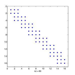
Figure 1: Shape of the modified matrix $T$ generated by Block_Lanczos

It is easily seen that under some genericity condition the modified matrix $T$ can be reduced by a diagonal unitary congruence into the CMV-shape described in Definition 1.2 in [14]. This explains why we refer to the matrix $T$ generated by the Block_Lanczos procedure as to a CMV–like form. Further, it is worth noticing that the computational cost of the Block_Lanczos algorithm amounts to perform a matrix-by-vector multiplication per step. Therefore, the overall cost is $O(nc_{m})$, where $O(c_{m})$ is the cost of multiplying the matrix $U+U^{H}\in\mathbb{C}^{n\times n}$ by a vector. In the case of the generator of the circulant matrix algebra, since the matrix $U$ is sparse, we get the complexity estimate $O(n^{2})$.

Some comments are however in order here. The first one is concerned with the applicability of the Block_Lanczos process devised above. Let us consider the Fourier matrix $U=\mathcal{F}_{n}=\frac{1}{\sqrt{n}}\Omega_{n}$ of order $n=2m$. Due to the relation $\Omega_{n}^{2}=n\Pi$, where $\Pi$ is a suitable symmetric permutation matrix, it is found that for any starting vector $\mathbf{z}$ the Block_Lanczos procedure breaks down within the first three steps. In this case the reduction scheme has to be restarted and the initial matrix can be converted into the direct sum of CMV-like blocks.

The second comment is that the profile shown in Figure 1 does not follow immediately from the rank-one property of the out-of-diagonal blocks. The observation is that after having performed the first two elementary transformations $T\rightarrow T_{1}=\mathcal{G}_{1}T\mathcal{G}_{1}^{H}$ and $T_{1}\rightarrow T_{2}=\mathcal{G}_{2}T_{1}\mathcal{G}_{2}^{H}$ determined so that $\hat{B}_{1}$ and $\tilde{B}_{1}^{H}$ are converted in the form displayed in Figure 1 then the subdiagonal block in position $(3,2)$ has already the desired shape due to the unitariness of the matrix $T_{2}$. In this way the reduction of $T$ can be completed by a sequence of Givens rotations only acting on the superdiagonal blocks in such a way to preserve the zero structure.

The final observation is that the reduction into the CMV–like shape has also a remarkable consequence in terms of rank structures of the resulting matrix. The property follows from a corollary (Corollary 3 in [12]) of a well known result in linear algebra referred to as the Nullity Theorem.

Theorem 3 (Nullity Theorem).

Suppose $A\in\mathbb{C}^{n\times n}$ is a nonsingular matrix and $\mathbf{\alpha}$ and $\mathbf{\beta}$ to be nonempty proper subsets of $J\colon=\{1,\ldots,n\}$. Then

$$\mbox{\rm{rank }}(A^{-1}(\mathbf{\alpha};\mathbf{\beta}))=\mbox{\rm{rank }}(A(J\setminus\mathbf{\beta};J\setminus\mathbf{\alpha}))+|\mathbf{\alpha}|+|\mathbf{\beta}|-n,$$

where, as usual, $|J|$ denotes the cardinality of the set $J$.

Now let $T\in\mathbb{C}^{n\times n}$, $n=2\ell$, denote a unitary matrix given in the CMV-like form shown in Figure 1. Set $\mathbf{\alpha}=\{1,2\}$ and $\mathbf{\beta}=\{5,\ldots,n\}$. Thus, we have

$$0=\mbox{\rm{rank }}(T(1\colon 2;5\colon n))=\mbox{\rm{rank }}(T^{H}(5\colon n;1\colon 2))=\mbox{\rm{rank }}(T(3\colon n;1\colon 4))-2,$$

which implies

$$\mbox{\rm{rank }}(T(3\colon n;1\colon 4))=2.$$

and, therefore,

$$\mbox{\rm{rank }}(T(3\colon 4;2\colon 3))=1$$

whenever $T(5:6,4)$ is nonzero. In fact, assume by contradiction that $\mbox{\rm{rank }}(T(3\colon 4;2\colon 3))=2$, then since by Corollary 1 $\mbox{\rm{rank }}(T(3\colon 4;1\colon 2))=1$, $\mbox{\rm{rank }}(T(5\colon:6,4:5))=1$ and the matrix is in CMV-like form, we obtain that $\mbox{\rm{rank }}(T(3:n,1:4))=3$ which is a contradiction. By similar reasonings we conclude that under the assumption that $T(2k+1:2(k+1),2k)$ is nonzero for $k=2,\ldots,\ell-1$ it is obtained that

$$\mbox{\rm{rank }}(T(2k+1\colon 2(k+1);2k\colon 2k+1))=1,\quad 1\leq k\leq\ell-2.$$ (8)

This property plays a fundamental role in the analysis of QR–based eigensolvers performed in Section 4.

3 A Householder style reduction algorithm

In this section we derive a Householder style reduction algorithm using elementary matrices to perform the transformation of a unitary matrix $U$ into the block tridiagonal form $T$. Let us recall that from (7) the unitary matrix $U$ is converted into the the block tridiagonal form $T$ by using a unitary congruence defined by the unitary matrix $Q$ whose first two columns are determined to generate the space $<\mathbf{z},U\mathbf{z}>$ for a suitable $\mathbf{z}\in\mathbb{C}^{n\times n}$. The rank properties of the out-of-diagonal blocks of $T$ stated in Corollary 1 enables the information of $T$ to be further compressed by using a sequence of Givens rotations in order to arrive at the form shown in Figure 1. The pattern of this sequence does not modify the first two column of $Q$.

A straightforward extension of the Implicit Q Theorem (see [13], Theorem 7.4.2) for block Hessenberg matrices indicates that essentially the same unitary matrix should be determined in any block tridiagonal reduction process by means of unitary transformations applied to $U+U^{H}$ provided that the first two columns of $Q$ span the space $<\mathbf{z},U\mathbf{z}>$. This suggests the alternative more stable procedure using unitary transformations outlined below. For the sake of simplicity we consider the case where $n$ is even.

Procedure Unitary_CMV_Reduction Input: $U$, $D_{0}=[\mathbf{z}|U\mathbf{z}]$; $[G,R]={\bf qr}(D_{0})$; $U=G^{H}UG$; $n={\bf length}(U)$; for $kk=1:n/2-2$ for $j=n:-1:2kk+3$     $Us=U(j-2:j,2kk-1:2kk)+(U(2kk-1:2kk,j-2:j))^{H}$;     $[Qs,Rs]={\bf qr}(Us)$;     $U(j-2:j,:)=Qs^{H}U(j-2:j,:)$;     $U(:,j-2:j)=U(:,j-2:j)Q_{s}$; end end

The complexity of this procedure is generally $O(n^{3})$. However there are some interesting structures which can be exploited. In particular, if $U$ is rank-structured then $U+U^{H}$ is also rank-structured and Hermitian so that the fast techniques developed in [11] might be incorporated in the algorithm above by achieving a quadratic complexity. The resulting fast version of the Unitary_CMV_Reduction algorithm will be presented elsewhere.

It is also worth noticing that for certain input data the algorithm above needs to be restarted if breakdown situations are detected. For instance, in Figure 2 we report the matrix generated by the algorithm Unitary_CMV_Reduction applied to the Fourier matrix of order 32. The $8\times 8$ block diagonal structure of the CMV–shape corresponds with 7 restarts of the algorithm. The 2-norm of the subdiagonal blocks corresponding to breakdowns are in the range $[2.3e-14,6.5e-14]$. The deflation criterion used in our implementation compares the 2-norm of the considered subdiagonal block with the bound $n\cdot{\rm u}\cdot\parallel U\parallel_{F}$, where u denotes the unit roundoff. This is justified by the fact that the Hessenberg reduction as well as QR iterations introduce roundoff errors of the same level [15].

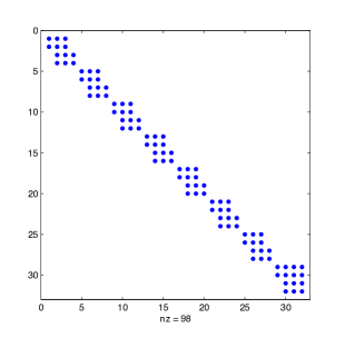
Figure 2: Block CMV reduction for the Fourier matrix of size $n=32$

4 Invariance of the CMV-like form under the QR algorithm

Our interest towards the reduction of unitary matrices into a CMV-like form stems from the unitary eigenvalue problem. In this respect it is mandatory to investigate the properties of CMV-like matrices under the QR algorithm which yields the customary approach for eigenvalue computation. The invariance of the CMV-like form under the QR iteration was firstly proved in the paper [5] using an algorithmic approach. The proof presented here is based on the property (8) and it has the advantage of admitting an immediate extension to almost unitary matrices.

Theorem 4.

Let $T_{0}=T\in\mathbb{C}^{n\times n}$, $n=2\ell$, be a unitary block tridiagonal matrix given in the CMV–like form shown in Figure 1. Moreover, let $T_{1}$ denote the matrix generated from one step of the QR algorithm with shift $\gamma$ , i.e.,

$$\left\{\begin{array}[]{ll}T_{0}-\gamma I_{n}=QR\quad({\rm QR}\ \ {\rm factorization});\\ T_{1}=RQ+\gamma I_{n}.\end{array}\right.$$

Assume that the subdiagonal blocks of both $T_{0}$ and $T_{1}$ are nonzero and that $T_{0}-\gamma I_{n}$ is nonsingular. Then the matrix $T_{1}$ is block tridiagonal with the same shape as $T_{0}$.

Proof.

From $T_{1}=RT_{0}R^{-1}$ where $R$ is upper triangular it follows that both the shape and the rank properties of the lower triangular portion of the matrix $T_{0}$ are preserved in the matrix $T_{1}$. Then by using Theorem 3 and property (8) we obtain that

$$\mbox{\rm{rank }}(T_{1}(1\colon 2;4\colon n))=\mbox{\rm{rank }}(T_{1}^{H}(4\colon n;1\colon 2))=\mbox{\rm{rank }}(T_{1}(3\colon n;1\colon 3))-1.$$

We have that $\mbox{\rm{rank }}(T_{1}(3\colon n;1\colon 3))=\mbox{\rm{rank }}(T_{0}(3\colon n;1\colon 3))=1$ as a consequence of the CMV-like structure of $T_{0}$ and for (8). This says that $T_{1}(1\colon 2;4\colon n)$ is a zero matrix. The same argument applies to any submatrix $T_{1}(1\colon 2s;2(s+1)\colon n)$, $1\leq s\leq\ell-2$, by yielding the CMV-like structure of $T_{1}$.

∎

The assumption about the invertibility of $T_{0}-\gamma I_{n}$ is just for the sake of simplicity. In the singular case we can get the same conclusion by a careful looking at the elementary transformations involved in the passage from $T_{0}$ to $T_{1}$ (compare with [7] for a general treatment of rank structures under the QR process in the singular case).

The conclusion of Theorem (4) immediately generalizes to almost unitary matrices of the form $A=U+\mathbf{z}\mathbf{w}^{H}$, with $U$ unitary, including the class of companion matrices. Indeed, if we apply the Unitary_CMV_Reduction to the matrix $U$ with initial vectors $\mathbf{z},U\mathbf{z}$, then it is shown that $U$ is reduced to CMV-like shape and simultaneously the rank-one correction is converted to a rank-one matrix with only the first nonzero row. In this way, the transformed matrix $B=Q^{H}AQ=T+\mathbf{e}_{1}\mathbf{v}^{H}$ is block upper Hessenberg with subdiagonal blocks of rank one. Setting $T_{0}=T$, $C_{0}=\mathbf{e}_{1}\mathbf{v}^{H}$, and applying a $QR$ step to matrix $B_{0}=B$, we have

$$B_{1}=T_{1}+C_{1},$$

where $T_{1}=Q^{H}T_{0}Q$ is unitary and $C_{1}=Q^{H}C_{0}Q$ is a rank one matrix. The following facts hold.

• Since the lower shape is maintained under the QR scheme, $B_{1}$ is block upper Hessenberg with subdiagonal blocks of rank one.

• $T_{1}$ has a rank–one structure in the lower triangular portion out of the diagonal blocks, due to the fact that $B_{1}$ is block Hessenberg with rank one subdiagonal blocks.

• $\mbox{\rm{rank }}(T_{1}(3:n,1:4))=3$, and for the Nullity Theorem, $\mbox{\rm{rank }}(T_{1}(1:2,5:n))=1$.

• Then, $\mbox{\rm{rank }}(B_{1}(1:2,5:n))\leq 2$.

This reasoning can be repeated at each $QR$ step obtaining that the matrix $B$ generated at each step has a rank–two structure in the upper triangular portion out of the block tridiagonal profile.

As an illustration of the structural properties of the CMV-like reduction under the QR process, we consider in Figure 5 the unitary matrix $T$ computed after 32 QR steps applied to the matrix $B$ determined from a companion matrix $A$ generated by the Matlab command ${\it compan}$. Specifically, we show the shape of the matrices $H$ and $S$ such that $T\cdot S=H$ and $S$ can be represented as product of a linear number of $2\times 2$ Givens rotation matrices. This factorization is an intermediate step in the computation of a QR factorization of $T$ [9] and clearly put in evidence the rank-one structure in the upper triangular portion of the matrix $T$.

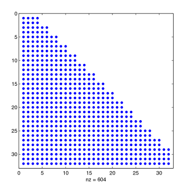
Figure 3: Shape of the matrix $H$

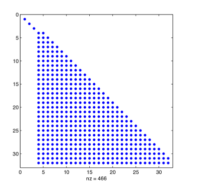
Figure 4: Shape of the matrix $S$

Figure 5: Illustration of the upper rank-one structure of $T$

5 Conclusion and future work

In this paper we have presented fast numerical methods for reducing a given unitary matrix into the direct sum of CMV-like matrices. The occurrence of potential rank structures in the matrix $U$ can be exploited by improving the computational cost of the reduction. As the resulting sparse representation of $U$ is invariant under the QR method the proposed reduction can naturally be applied for the fast solution of the unitary rank structured eigenvalue problems.

Some theoretical and computational issues are currently being investigated. A first interesting question is related with the completion problem for unitary matrices whose block lower Hessenberg profile is only known (compare with [4]). Other issues concern the numerical treatment, representation and compression of out-of-band semiseparable unitary matrices [10]. In particular, the rank–one structure of the matrices generated under the QR method applied to a transformed companion matrix can provide an easy, numerically efficient representation to be exploited for the design of fast matrix–based polynomial rootfinding methods. The preliminary transformation of a companion matrix into a perturbed CMV-like form can provide alternative algorithms with better numerical and computational features.

References

- [1] G. S. Ammar, W. B. Gragg, and C. He. An efficient QR algorithm for a Hessenberg submatrix of a unitary matrix. In New directions and applications in control theory, volume 321 of Lecture Notes in Control and Inform. Sci., pages 1–14. Springer, Berlin, 2005.
- [2] D. A. Bini, Y. Eidelman, L. Gemignani, and I. Gohberg. Fast QR eigenvalue algorithms for Hessenberg matrices which are rank-one perturbations of unitary matrices. SIAM J. Matrix Anal. Appl., 29(2):566–585, 2007.
- [3] D. A. Bini, Y. Eidelman, L. Gemignani, and I. Gohberg. The unitary completion and QR iterations for a class of structured matrices. Math. Comp., 77(261):353–378, 2008.
- [4] D. A. Bini, Y. Eidelman, L. Gemignani, and I. Gohberg. The unitary completion and QR iterations for a class of structured matrices. Math. Comp., 77(261):353–378, 2008.
- [5] A. Bunse-Gerstner and L. Elsner. Schur parameter pencils for the solution of the unitary eigenproblem. Linear Algebra Appl., 154/156:741–778, 1991.
- [6] M. J. Cantero, L. Moral, and L. Velázquez. Five-diagonal matrices and zeros of orthogonal polynomials on the unit circle. Linear Algebra Appl., 362:29–56, 2003.
- [7] S. Delvaux and M. Van Barel. Rank structures preserved by the -algorithm: the singular case. J. Comput. Appl. Math., 189(1-2):157–178, 2006.
- [8] S. Delvaux and M. Van Barel. Eigenvalue computation for unitary rank structured matrices. J. Comput. Appl. Math., 213(1):268–287, 2008.
- [9] Y. Eidelman and I. Gohberg. A modification of the Dewilde-van der Veen method for inversion of finite structured matrices. Linear Algebra Appl., 343/344:419–450, 2002. Special issue on structured and infinite systems of linear equations.
- [10] Y. Eidelman and I. Gohberg. Out-of-band quasiseparable matrices. Linear Algebra Appl., 429(1):266–289, 2008.
- [11] Y. Eidelman, I. Gohberg, and L. Gemignani. On the fast reduction of a quasiseparable matrix to Hessenberg and tridiagonal forms. Linear Algebra Appl., 420(1):86–101, 2007.
- [12] M. Fiedler and T. L. Markham. Completing a matrix when certain entries of its inverse are specified. Linear Algebra Appl., 74:225–237, 1986.
- [13] G. H. Golub and C. F. Van Loan. Matrix computations. Johns Hopkins Studies in the Mathematical Sciences. Johns Hopkins University Press, Baltimore, MD, third edition, 1996.
- [14] R. Killip and I. Nenciu. CMV: the unitary analogue of Jacobi matrices. Comm. Pure Appl. Math., 60(8):1148–1188, 2007.
- [15] F. Tisseur. Backward stability of the QR algorithm. Technical Report 239, UMR 5585 Lyon Saint-Etienne, 1996.
- [16] R. Vandebril and D. S. Watkins. An extension of the qz algorithm beyond the hessenberg-upper triangular pencil. Electronic Transactions on Numerical Analysis, 40:17–35, 2013.
- [17] T. L. Wang and W. B. Gragg. Convergence of the shifted algorithm for unitary Hessenberg matrices. Math. Comp., 71(240):1473–1496, 2002.
- [18] T. L. Wang and W. B. Gragg. Convergence of the unitary QR algorithm with a unimodular Wilkinson shift. Math. Comp., 72(241):375–385, 2003.