Novel techniques to search for neutron radioactivity

Abstract

Two new methods to observe neutron radioactivity are presented. Both methods rely on the production and decay of the parent nucleus in flight. The relative velocity measured between the neutron and the fragment is sensitive to half-lives between $\sim$1 and $\sim$100 ps for the Decay in Target (DiT) method. The transverse position measurement of the neutron in the Decay in a Magnetic Field (DiMF) method is sensitive to half-lives between 10 ps and 1 ns.

1 Introduction

Nuclei with extreme neutron deficiency or neutron excess can decay by the emission of one or more protons or neutrons, respectively. The presence of the Coulomb barrier can significantly hinder the emission of a proton which can lead to fairly long lifetimes for this decay mode. The current status of one- and two-proton radioactivity has recently been reviewed by Pfützner [1]. In contrast, neutron emission typically proceeds on very short time scales ($\sim$10^-21 s), primarily due to the absence of the Coulomb barrier. However, it has been postulated that in special cases one- or two-neutron radioactivity might occur due to the presence of an angular momentum barrier [2, 3, 4]. Lifetimes as short as 10^-12 s can be considered as radioactivity [5] and only in the most extreme cases neutron emission is expected to reach these time scales. Thus traditional methods where the decaying nucleus is implanted in a detector and the subsequent decay is recorded are not applicable. With these methods the shortest measured lifetimes at present are 620 ns [6, 7] and 1.9 $\mu$s [8, 9, 10] for $\alpha$- and proton-decay, respectively.

Mukha et al. developed a new technique to measure the two-proton decay of ¹⁹Mg in flight by tracking the paths of the decay products and measured a half-life of 4.0(15) ps [11]. Voss et al. studied the same decay with an adaptation of the recoil distance method. The degrader foil of a plunger device was replaced by a double-sided silicon strip detector to measure the energy-loss of the decaying nucleus (¹⁹Mg) and the resulting fragment (¹⁷Ne). The lifetime was then extracted from the intensity ratio of the energy loss peaks as a function of target to detector distance [12].

In order to search for the corresponding decays of neutron-rich nuclei these or similar techniques have to be developed for neutron emission. Grigorenko et al. suggested one might adapt the tracking method by measuring the angular distributions of the neutron(s) and the fragment with high precision [3]. The reconstructed opening angle of the decay is then directly related to the decay energy. Caesar et al. extracted an upper limit of 5.7 ns for the decay of ²⁶O by two-neutron emission by assuming the survival of ²⁶O along the flight path in a magnetic field [13]. For future experiments they also proposed placing the target directly in front of a deflecting magnet and then deducing the lifetime from the horizontal position distribution of the neutrons. Most recently Kohley et al. applied another modification of the recoil distance method to analyze the previously reported ground-state two-neutron decay of ²⁶O [14]. In this method the velocity difference between the neutrons and the fragments is sensitive to the lifetime if the decay occurs within the target. A half-life of 4.5${}^{+1.1}_{-1.5}$(stat)$\pm$3(syst) ps was determined for the decay of ²⁶O [15].

In the present paper we discuss calculations to extract the half-life sensitivities of the two methods mentioned above: the velocity difference method for the Decay in the Target (DiT) and the method to measure the horizontal neutron position distribution following the Decay in a Magnetic Field (DiMF).

2 Test case of ¹⁶B

In order to explore the feasibility of the DiT and DiMF methods for the measurement of neutron radioactivity, the single neutron decay of ¹⁶B was used as a test case. Although it is unlikely that neutron radioactivity will be observed in ¹⁶B, the reaction ¹⁷C(-p)¹⁶B$\rightarrow^{15}$B + n was simulated because the complications due to the emission of multiple neutrons, occurring in the potentially more interesting case of the two-neutron emitter ²⁶O, are avoided.

¹⁶B is unbound with respect to ¹⁵B plus a neutron [16, 17] and the ground state resonance was reported at 40(60) keV [19] and 40(40) keV [18] from multiparticle transfer reactions. Such a low decay energy (which is consistent with 0 keV within the given uncertainty) is critical for the possible observation of a finite lifetime because of the small barrier which is only due to the angular momentum. For an $l$=2 transition, which is expected for the ground state of ¹⁶B, a decay energy of about 1 keV corresponds to a half-life of approximately 0.1 ps [2, 4]. Subsequently, invariant mass measurements found a resonance at low decay energies of 85(15) keV [20] and 60(20) keV [21]. This resonance most likely corresponds to the ground state decay. However, it is still conceivable that it could be a transition to one of the bound excited states of ¹⁵B. In an attempt to search for neutron radioactivity of ¹⁶B an upper limit for the half-life of 132 ps (68% confidence level) was extracted from a proton stripping reaction from a radioactive ¹⁷C beam [2].

3 Decay in Target (DiT)

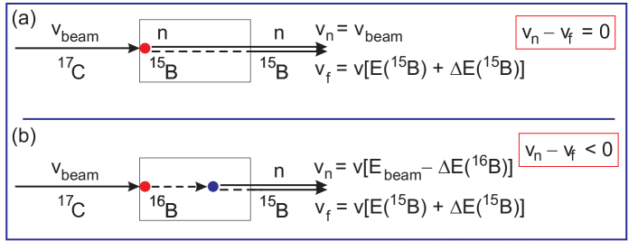
Figure 1: Schematics of the DiT technique. Panel (a) shows the production of ¹⁶B and decay to ¹⁵B and a neutron at the beginning of the target, while in panel (b) ¹⁶B is produced at the beginning of the target but decays to ¹⁵B and a neutron at a later time in the target. Because the position of the decay is unknown, $\Delta$E(¹⁵B) is calculated assuming it traverses the whole target. The calculations of the relevant velocities are explained in the text.

The DiT technique was recently applied for the first time in the decay of ²⁶O into ²⁴O and two neutrons [15]. A schematic overview of this technique is shown in figure 1 for the decay of ¹⁶B as an example. In this figure it is assumed that the one-proton removal reaction ¹⁷C(-p)¹⁶B occurs at the beginning of the target and the outgoing fragment continues with essentially the same velocity as the incoming beam. As mentioned before, in order for long lifetimes to occur the decay energy for the subsequent decay of ¹⁶B into ¹⁵B and a neutron has to be very low and therefore recoil effects can be neglected. Panel (a) of the figure depicts the situation where the decay of ¹⁶B into ¹⁵B and a neutron proceeds instantaneously. While the neutrons continue at beam velocity through the target and into the neutron detectors, the ¹⁵B fragments lose energy as they traverse the target before the final energy is measured with charged-particle detectors. The fragment velocity at the interaction point can then be reconstructed from the measured final energy [E(¹⁵B)] and the energy loss through the target [$\Delta$E(¹⁵B)] which can be calculated with the above assumptions from the incoming beam energy and the target thickness. The velocity difference v${}_{n}-$ v_f for this case is then equal to zero. If the decay occurs at a later time, when the ¹⁶B fragment has traveled through a fraction of the target, the calculated velocity difference will be less than zero as shown in figure 1(b). As the location of the decay is unknown, the fragment velocity is calculated with the assumption that the decay occurred at the beginning of the target, the same as in panel (a). The neutron velocity, however, will be reduced due to the energy loss of the ¹⁶B in the target before its decay to ¹⁵B and the neutron. The signature for a finite lifetime of the decay is thus a shift towards negative values of the velocity difference v${}_{n}-$ v_f.

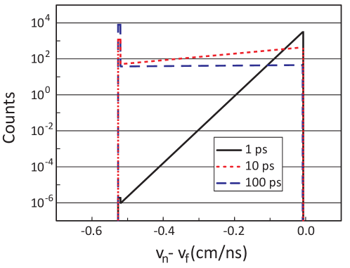
Figure 2: Velocity difference distributions for the decay of ¹⁶B into ¹⁵B and a neutron at 80 MeV/u for three different half lives. The production of ¹⁶B is assumed to occur at the beginning of a 700 mg/cm^{2 9}Be target. The fragment velocity was calculated after adding the energy loss of the fragment through the whole target to the final measured energy.

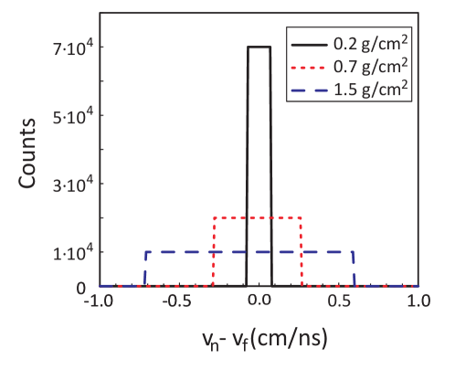
Figure 3: Velocity difference distributions from the instantaneous decay of ¹⁶B (t_1/2 = 0 ps) to ¹⁵B for three different target thicknesses at an incident beam energy of 80 MeV/u. For these curves it was assumed that ¹⁶B could be produced (and decay instantaneously) anywhere equally distributed throughout the target. The energy loss of the fragments through only half the target was added back to the final measured fragment energy in order to center the velocity difference distributions at v${}_{n}-$ v${}_{f}\sim 0$.

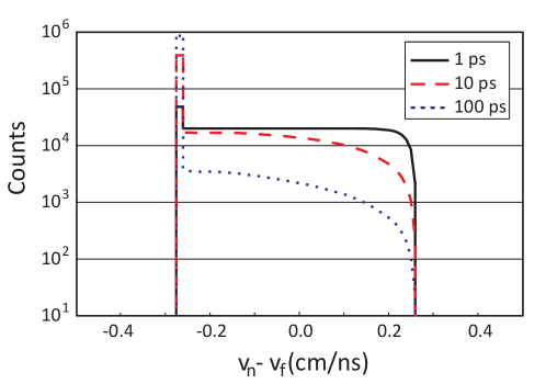
Figure 4: Same as figure 2 assuming that the production can occur anywhere in the target, i.e. the curves from figure 2 were folded with the spread to the energy loss in the target shown by the red/dotted line (700 mg/cm²) from figure 3.

The various effects contributing to the measured distributions are demonstrated in figures 2-5. Figure 2 shows the calculated velocity difference assuming that ¹⁶B is produced at the beginning of the target. Distributions for half-lives of 1 ps (black/solid line), 10 ps (red/dotted line), and 100 ps (blue/dashed line) are shown for a 700 mg/cm² thick ⁹Be target and an incoming ¹⁷C beam energy of 80 MeV/u. For the calculation of the velocity difference the energy loss through the full target was added back to the final fragment energy. The exponential decrease of the velocity difference translates directly to the half life. The beam energy corresponds to a velocity of 11.7 cm/ns and with a target thickness of 0.38 cm, the traversal time through the target is $\sim$32 ps. The decay rate for a half-life of 10 ps drops by about an order of magnitude during this time, consistent with the decrease shown by the red/dotted line in the figure. The sharp increase at the left edge of the distributions is due to the integral of decays outside of the target which is larger for the longer half-lives.

More realistic calculations have to take into account that the reaction can take place anywhere in the target. Because the exact interaction point is unknown, the velocity difference broadens due to the varying energy losses by the fragments in the target. This effect is shown in figure 3 for target thicknesses of 200 mg/cm² (black/solid line), 700 mg/cm² (red/dotted line), and 1500 mg/cm² (blue/dashed line). The beam energy was 80 MeV/u and it was assumed that the subsequent decay occurs at the same time/place as the reaction (t_1/2 = 0 ps). In order to center the distributions at v${}_{n}-$ v_f = 0, only the energy loss through half the target thickness was added back to the final fragment energy.

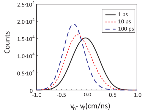
Figure 5: Same as figure 4 folded with the resolution of the velocity measurements.

The combined effect of finite half-lives and uniform distribution of the reaction within the target is shown in figure 4 for the same three half-lives and conditions as in figure 2. Finally, the results of the simulations have to be folded with realistic resolutions of the detectors. The corresponding curves displayed in figure 5 were calculated with an overall resolution of 0.2 cm/ns which assumed resolutions (FWHM) of 2% and 3% for the neutron and charged particle detectors, respectively [15]. The distributions for the half-lives shown in the figure demonstrate the approximate limits of the method. While the velocity difference distribution for a half-life of 1 ps is essentially centered around zero, the distribution for a half-life of 100 ps is centered at the edge of the target and distributions for longer half-lives are very similar.

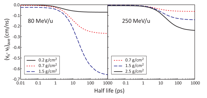
Figure 6: Average value of the velocity difference distributions for the DiT technique as a function of half-life using the reaction ¹⁷C(-p)¹⁶B$\rightarrow$¹⁵B+n at 80 MeV/u (left) and 250 MeV/u (right) for three different target thicknesses.

The general sensitivity of the method can be shown by plotting the average value of the folded velocity difference distributions as a function of half-lives. Figure 6 shows the dependence on the target thickness for incident beam energies of 80 MeV/u (a) and 250 MeV/u (b). The thicker targets are more sensitive because the velocity difference depends on the energy loss of the charged fragments in the target. For the same reason, the method is also more effective at lower energies for the same target thickness.

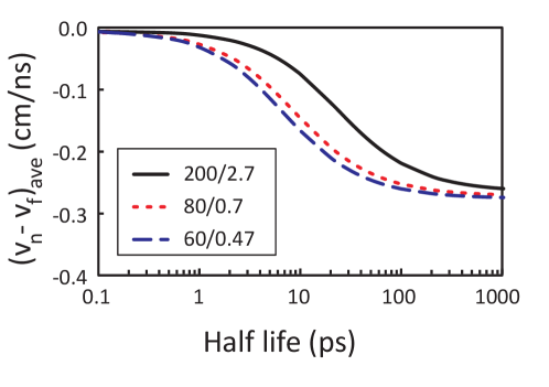
Figure 7: Average value of the velocity difference distributions for the DiT technique as a function of half-life for the reaction ¹⁷C(-p)¹⁶B$\rightarrow$¹⁵B+n and three different combinations of beam energy and target thicknesses. The first number in the legend corresponds to the beam energy in MeV/u and the second number is the target thickness in g/cm².

The choice of target thickness for a given energy is limited by the requirement that the remaining energy after the target has to be sufficiently large to allow for a clean identification of the fragment and a good energy measurement ($\sim$3% in velocity, see above). Thus at higher energies, thicker targets can be used. Nevertheless, in order to push the methods to the smallest half-lives it is still advantageous to use lower beam energies as shown in figure 7. The target thicknesses of 2700 mg/cm², 700 mg/cm², and 470 mg/cm² for beam energies of 200 MeV/u (black/solid line), 80 MeV/u (red/dotted line), and 60 MeV/u (blue/dashed line), respectively, were selected to reach approximately the same asymptotic value for very long half-lives.

In addition to the target thickness and beam energy, the design of an experiment to search for neutron radioactivity has to consider other factors such as available beam intensity, reaction cross sections and detector resolution. The most important factor in order to extract a reasonable measurement of a half-life will most likely be statistics. At the present time, the beam intensities for very neutron-rich radioactive beams are still relatively small, although the new RIBF at RIKEN [22] has achieved some impressive increases. A recent experiment to study the two-neutron decay of ²⁶O with the SAMURAI/NEBULA setup collected about a factor of 30 more statistics [23] than the published data from MSU/NSCL [15]. However, the experiment was performed at a higher incident beam energy (200 MeV/u) with a thicker target (2 g/cm²) and it is not clear if the increased statistics will be sufficient to make up for the reduction in sensitivity in the $\sim$4 ps range (see figure 7). If the beam energy at RIBF can be reduced without significant intensity losses SAMURAI/NEBULA is in the ideal position to improve on the lifetime measurement of ²⁶O.

4 Decay in Magnetic Field

Figure 8: Schematics of the DiMF technique. The incoming ¹⁷C beam produces ¹⁶B in the target (red dot) which enters a magnet field (bend radius $r$ and deflection angle $\theta$) after a drift distance $d$. ¹⁶B then can decay at different positions along the flight path (blue dots) into ¹⁵B and a neutron. The ¹⁵B fragments and neutrons are detected and identified in a set of charged-particle detectors and position sensitive scintillation detectors (at a distance $l$ from the target), respectively.

An alternative method to measure finite lifetimes of neutron emitters proposed by Caesar et al. involves the deflection of the fragments in a magnetic field after the target and measuring the position distribution of the neutrons [13]. A schematic overview of such an experiment is shown in figure 8. The reaction [¹⁷C(-p)¹⁶B] takes place in the target (red dot) and the subsequent decay (¹⁶B$\rightarrow^{15}$B + n) can occur at later times in-flight (blue dots). A deflecting magnetic field with a bend radius $r$ and a deflecting angle $\theta$ bends the charged particles away from zero degrees after a possible drift distance $d$ into a set of charged-particle detectors. The neutrons are typically detected with an array of scintillation detectors [24, 25, 26, 27] located near zero degrees at a distance $l$ from the target. If the lifetime is sufficiently long for ¹⁶B to decay within the magnetic field, the horizontal distribution of the neutrons along the detector is directly related to the half-life.

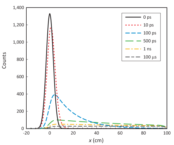
Figure 9: Transverse position distributions for neutrons from the reaction ¹⁷C(-p)¹⁶B$\rightarrow$¹⁵B+n at 200 MeV/u for different half-lives. The drift distance, bend radius and neutron detector distances were 0 cm, 200 cm, and 1500 cm, respectively.

Figure 9 shows these distributions for six different half-lives. The calculations were performed at a beam energy of 200 MeV/u and a bend radius of 2 m. The drift distance was 0 cm and 2-m long neutron detectors were placed at a distance of 15 m from the target and centered at the beam axis. The results were folded with a position resolution of 3 cm.

Short lifetimes ($\lesssim$10 ps) result in a shift of the peak of the distributions, while for longer lifetimes, the exponential decay is directly proportional to an exponential position decay across the detector which can be expressed by a position decay constant: $\lambda_{x}$= $-$ln($\Delta$(Counts))/$\Delta$x). The optimum sensitivity for this arrangement is about 100 ps, where – depending on the statistics of the experiment – half-lives as short as 10 ps and as long as 1 ns might be measurable.

Similar to the DiT technique, in the actual experiment the half-life has to be extracted from a detailed fit to the whole distribution taking all experimental parameters into account. However, the sensitivity range of the DiMF method can be explored by analyzing the average value of the position distributions ($x_{ave}$) and the position decay constant $\lambda_{x}$ which are shown as a function of half-lives in the top and bottom panel of figure 10, respectively.

The parameters for the three lines shown were selected as approximate representations of the experimental setups Sweeper-MoNA at MSU/NSCL (black/solid) [30, 31], SAMURAI-NEBULA at RIKEN/RIBF (red/dotted) [28], and R³B-NeuLAND at FAIR (blue/dashed) [27, 29]. The Sweeper-MoNA calculations were performed for an incoming beam energy of 80 MeV/u, a bend radius of 1 m, and a target to MoNA distance of 8 m. Calculations for the SAMURAI-NEBULA setup assumed a beam energy of 200 MeV, a bend radius of 2 m and a neutron time-of-flight distance of 15 m. The corresponding values for R³B-NeuLAND were 450 MeV/u, 4 m and 35 m. It should be stressed that for all calculations the target was placed directly in front of the magnet with a drift distance of 0 m.

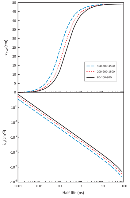
Figure 10: Average position $x_{ave}$ (top) and position decay constant $\lambda_{x}$ (bottom) of the transverse position distributions for neutrons from the reaction ¹⁷C(-p)¹⁶B$\rightarrow$¹⁵B+n as a function of half-lives. The numbers in the legend box correspond to the incoming beam energy in MeV/u, bend radius in cm, and neutron detector distance in cm.

The most important parameter to reach sensitivities for short lifetimes is the beam energy. However, even at the highest beam energies it will be difficult to reach sensitivities below about 10 ps. The bend radius and the neutron time-of-flight distance are directly proportional, i.e. for a given beam energy a bend radius of 1 m and detector distance of 5 m is equivalent to a radius of 3 m and a distance of 15 m.

While $x_{ave}$ is more sensitive to shorter lifetimes, $\lambda_{x}$ is more relevant for longer lifetimes. The sensitivity limits can be estimated by comparing the red curves in figure 10 with the approximate parameters for the SAMURAI-NEBULA setup with the distributions of figure 9 which were calculated with the same parameters. The lower limit for extracting a half-life of $\sim$10 ps is determined from the lower limit of measuring the shift of $x_{ave}$ at about 2 cm, while the upper limit of $\sim$1 ns is due the limit of measuring $\lambda_{x}$ at about $-$0.01 cm^-1.

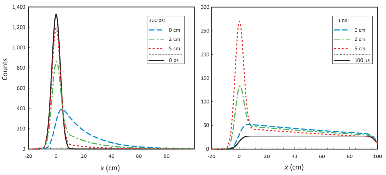
Figure 11: Transverse position distributions for neutrons from the reaction ¹⁷C(-p)¹⁶B$\rightarrow$¹⁵B+n at 200 MeV/u and half-lives of 100 ps (left) and 1 ns (right). Distributions for drift distances of 0 cm (blue/dashed line) 2 cm (green/dot-dashed line) and 5 cm (red/dotted line) are shown. For reference, the distributions for half-lives of 0 ps and 100 $\mu$s for 0 cm drift distance (black/solid line) are included in the left and right panel, respectively. The calculations were performed for the same number of reactions. Note the difference in the vertical scales.

The importance of placing the target directly in front of the deflecting magnet is demonstrated in figure 11. Especially for the shorter lifetimes, it will be critical to locate the target as close as possible to the magnet. As shown in the left panel of the figure, for a half-life of 100 ps a drift distance as small as 2 cm already moves the peak of the distribution to the center with only a tail extending to larger distances. For longer lifetimes the drift distance is not as critical. Although a certain fraction of the events will accumulate in a peak at the center, the position decay constant of the distribution remains the same and the overall intensity of the tail is not significantly reduced (see the right panel of the figure).

5 Conclusions

Two methods to search for neutron radioactivity were discussed. In the first method the velocity difference of the neutrons and the charged fragments is measured. This method is sensitive to decays that occur within the target (DiT) and depends on the energy loss of the charged fragment in the target. The second method is sensitive to decays in-flight after the target by relying on the deflection of the charged fragment in a magnetic field (DiMF) which will then translate into the horizontal distribution of the neutrons. In order to be sensitive to the shortest lifetimes, the DiT method is better at low beam energies while the DiMF method is more sensitive at high beam energies. Within the range of presently available beam energies and experimental setups the DiT method is more sensitive to half-lives in the 1–100 ps range, while the DiMF method is sensitive to half-lives between $\sim$10 ps and $\sim$1 ns.

References

- [1] M. Pfützner, Phys. Scr. T152, 014014 (2013)
- [2] R. A. Kryger et al., Phys. Rev. C 53, 1971 (1996)
- [3] L. V. Grigorenko, I. G. Mukha, C. Scheidenberger, and M. V. Zhukov, Phys. Rev. C 84, 021303(R) (2011)
- [4] T. Baumann, A. Spyrou, M. Thoennessen, Rep. Prog. Phys. 75, 036301 (2012)
- [5] M. Thoennessen, Rep. Prog. Phys. 67, 1187 (2004)
- [6] S. N. Liddick et al., Phys. Rev. Lett. 97, 082501 (2006)
- [7] R. Grzywacz et al., Nucl. Instrum. Meth. B 261, 1103 (2007)
- [8] C. R. Bingham et al., Nucl. Instrum. Meth. B 241, 185 (2005)
- [9] R. Grzywacz et al., Eur. Phys. J. A 25, s01, 145 (2005)
- [10] K. P. Rykaczewski et al., AIP Conf. Proc. 764, 223 (2005)
- [11] I. Mukha et al., Phys. Rev. Lett. 99, 182501 (2007)
-
[12]
P. Voss et al., subm. to Phys. Rev. C, P. Voss, Recoil distance method lifetime measurements via gamma-ray and charged-particle spectroscopy at NSCL, Ph. D. thesis, Michigan State University, unpublished (2011),
http://www.nscl.msu.edu/ourlab/publications/download/Voss2011_278.pdf - [13] C. Caesar et al., arXiv:1209.0156v2
- [14] E. Lunderberg et al., Phys. Rev. Lett. 108, 142503 (2012)
- [15] Z. Kohley et al., Phys. Rev. Lett. 110, 152501 (2013)
- [16] J. D. Bowman, A. M. Poskanzer, R. G. Korteling, and G. W. Butler, Phys. Rev. C 9, 836 (1974)
- [17] M. Langevin et al., Phys. Lett. B 150, 71 (1985)
- [18] R. Kalpakchieva et al., Eur. Phys. J. A 7, 451 (2000)
- [19] H. G. Bohlen et al., Nucl. Phys. A 583, 775c (1995)
- [20] J.-L. Lecouey et al., Phys. Lett. B 672, 6 (2009)
- [21] A. Spyrou et al., Phys. Lett. B 683, 129 (2010)
- [22] Y. Yano, Nucl. Instrum. Meth. B 261, 1009 (2007)
- [23] Y. Kondo et al., 4th International Conference on Collective Motion in Nuclei under Extreme Conditions COMEX4, October 22–26, 2012, Shonan Village Center, Kanagawa, Japan; T. Nakamura, private communication
- [24] T. Blaich et al., Nucl. Instrum. Meth. A 314, 136 (1992)
- [25] T. Baumann et al. , Nucl. Instrum. Meth. A 543, 517 (2005)
- [26] K. Yoneda et al., RIKEN Accel. Prog. Rep. 43, 178 (2010)
-
[27]
Technical Report for the Design, Construction and Commissioning of NeuLAND: The High-Resolution Neutron Time-of-Flight Spectrometer for R3B,
http://www.fair-center.eu/fileadmin/fair/experiments/NUSTAR/Pdf/TDRs/NeuLAND-TDR-Web.pdf -
[28]
Large-Acceptance Multi-Particle Spectrometer SAMURAI, Presentation at RIBF TAC05, RIKEN, Japan, 17–19 November 2005
http://ribf.riken.go.jp/RIBF-TAC05/10_SAMURAI.pdf - [29] B. Gastineau et al., IEEE Trans. Appl. Supercond. 18, 407 (2008)
- [30] M. D. Bird et al., IEEE Trans. Appl. Supercond. 15, 1252 (2005)
- [31] Z. Kohley et al., Nucl. Instrum. Meth. A 682, 59 (2012)