A renormalization group study of persistent current in a quasiperiodic ring

Abstract

We propose a real-space renormalization group approach for evaluating persistent current in a multi-channel quasiperiodic fibonacci tight-binding ring based on a Green’s function formalism. Unlike the traditional methods, the present scheme provides a powerful tool for the theoretical description of persistent current with a very high degree of accuracy in large periodic and quasiperiodic rings, even in the micron scale range, which emphasizes the merit of this work.

The observation of non-decaying circular current in a metallic ring in presence of Aharonov-Bohm (AB) flux is one of the noteworthy phenomena in mesoscopic physics. The measurement of low-temperature magnetic response of $10^{7}$ isolated mesoscopic copper rings to a slowly varying magnetic flux by Levy et al. levy in 1990 was the first experimental evidence of flux-periodic persistent current though the theoretical prediction was made much earlier in 1983 by Büttiker et al. butt1 . Later, many theoretical butt2 ; gefen ; san1 ; san2 ; san3 ; san4 as well as experimental mailly1 ; mailly2 ; mailly3 ; blu attempts were made to understand the intricate role of electron-electron interaction, disorder and quantum interference on the phenomenon of persistent current. These studies are mostly confined to mesoscopic systems, but interesting recent possibilities are that micron scale DNA loops also support persistent current nakamae ; kim . The DNA’s are large biopolymers consisting of thousands of atoms and exhibit both the periodic as well as quasiperiodic arrangement of the base pairs guo ; diaz ; macia1 ; macia2 . The quasiperiodic arrangements macia3 ; shechtman (e.g. fibonacci sequence), lacking of translational invariance, possess certain kind of long-range order leading to self-similar structures snk1 and a number of elegant real-space renormalization group (RSRG) techniques were proposed to understand the unusual physical properties of quasiperiodic systems kohmoto1 ; kohmoto2 ; snk2 ; snk3 ; snk4 ; snk5 ; lu . Apart from the periodic ladder models, the quasiperiodic fibonacci ladder network (see Fig. 1) has also been widely used in modeling the double-stranded DNA structure to study its electronic structure, charge transfer, etc. The sensitivity of persistent current of a $1$D fibonacci ring to Fermi energy was investigated by some groups jin ; hu calculating persistent current from the derivative of ground state energy of the system with respect to the applied magnetic flux. The studies on persistent current in the double-stranded circular DNA of higher organisms is highly limited kim , and the loop geometry of quasiperiodic fibonacci ladder network has yet to be investigated. A major problem for such biopolymers is that the system size is very large, one needs to diagonalize big matrices, and the numerical errors make it difficult to predict persistent current form the derivative of the ground state energy with respect to magnetic flux.

To overcome this problem, in the present communication we propose a RSRG technique snk2 ; snk3 for the evaluation of persistent current in a large quasiperiodic multi-channel ring. As an illustrative example of a quasiperiodic multi-channel ring, here we consider a fibonacci ladder rolled in the form of a loop. The key idea is that first we introduce the concept of

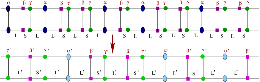
Figure 1: (Color online). Upper panel: A typical realization of an $8$-th generation fibonacci ladder composed of long ($L$) and short ($S$) bonds, where the sites between $L$-$L$, $L$-$S$ and $S$-$L$ bonds are labeled by $\alpha$, $\beta$, and $\gamma$, respectively. Lower panel: A one step renormalized version of the ladder.

the density of persistent current (DOPC) in terms of the retarded and advanced Green’s functions, then using RSRG method we replace the original large loop by an effective loop consisting of only few effective atoms, and finally calculate DOPC from the Hamiltonian of the effective ring. This method is numerically very efficient since it involves only the iteration of few recursion relations of the system parameters and requires the inverse of small matrices in order to find the retarded and advanced Green’s functions, and finally yields persistent current with a very high degree of accuracy.

We now describe our RSRG method for determination of persistent current in a quasiperiodic fibonacci ladder network in the form of a ring in which persistent current is induced by applying an infinitesimally slowly varying magnetic flux $\phi$ through the ring. This method can easily be employed to any periodic or quasiperiodic systems possessing self-similarity. In order to implement the RSRG scheme, we have to start with a general model for the fibonacci ladder network as illustrated in Ref. snk2 and the ring shape geometry is enforced by imposing periodic boundary condition. A schematic diagram of a general quasiperiodic fibonacci ladder network is depicted in Fig. 1. In the general model two types of bonds, namely, long ($L$) and short ($S$) bonds are arranged according to the quasiperiodic fibonacci sequence, and, we have three different kinds of atomic sites, $\alpha$, $\beta$ and $\gamma$, corresponding to the $L$-$L$, $L$-$S$, and $S$-$L$ vertices, respectively. Construction of the fibonacci sequence $\{F_{g}\}$ of generation $g$ is based on the rule $\{F_{g}\}$=$\{F_{g-1},F_{g-2}\}$ for $g\geq 3$ with $F_{1}=S$ and $F_{2}=L$. Each strand of the ladder is constructed exactly with the same fibonacci sequence of some particular generation. In Fig. 1, ladders corresponding to two successive generations of the quasiperiodic sequence are displayed where the three different geometrical shapes oval, square and circle represent the $\alpha$, $\beta$ and $\gamma$ atomic sites, respectively.

Within a tight-binding (TB) framework, the Hamiltonian of the fibonacci multi-channel ring threaded by a magnetic flux $\phi$ (in unit of the elementary flux quantum $\phi_{0}=hc/e$) reads,

$$\mbox{\boldmath$H$}=\sum_{i=1}^{N_{g}}\mbox{\boldmath$c$}_{i}^{{\dagger}}\mbox{\boldmath$\varepsilon$}_{i}\mbox{\boldmath$c$}_{i}+\sum_{i=1}^{N_{g}}(e^{j\theta_{i,i+1}}\mbox{\boldmath$c$}_{i}^{{\dagger}}\mbox{\boldmath$\tau$}_{i,i+1}\mbox{\boldmath$c$}_{i+1}+h.c.)$$ (1)

where,

$$\mbox{\boldmath$\varepsilon$}_{i}=\left(\begin{array}[]{c c}\epsilon_{i}~{}~{}v\\ v~{}~{}\epsilon_{i}\end{array}\right),\mbox{\boldmath$\tau$}_{i,i+1}=\left(\begin{array}[]{c c}t_{i,i+1}~{}~{}d_{i,i+1}\\ d_{i,i+1}~{}~{}t_{i,i+1}\end{array}\right),\mbox{\boldmath$c$}_{i}=\left(\begin{array}[]{c}c_{i,I}\\ c_{i,II}\end{array}\right).$$ (8)

Here, $v$ is the vertical hopping between the $i$-th sites of the two different strands I and II of the ladder and $N_{g}$ is the total number of sites of $g$-th generation of fibonacci lattice. The hopping integrals $t_{i,i+1}$ along each strand of the ladder has two values $t_{L}$ and $t_{S}$, corresponding to the long and short bonds respectively. Here, $d_{i,i+1}$ represents diagonal hopping between dissimilar sites of the two strands. The electron creation (annihilation) operators in the Wannier basis $|iI\rangle$ and $|iII\rangle$ are $c_{iI}^{{\dagger}}$ ($c_{iI}$) and $c_{iII}^{{\dagger}}$ ($c_{iII}$), respectively. The phase factor $\theta_{i,i+1}$ is set to $2\pi a_{i,i+1}\phi/\Lambda$, where $a_{i,i+1}=a_{L}$ or $a_{S}$ represents the long or short bond lengths respectively and $\Lambda=\sum\limits_{i=1}^{N_{g}}a_{i,i+1}$ is the perimeter of the ring.

In order to implement the RSRG scheme, we first express persistent current in terms of the Green’s function of the system. This has been achieved by introducing the notion of the density of persistent current $J(E)$ such that $J(E)dE$ gives the amount of persistent current in the energy interval between $E$ and $E+dE$. From the standard expression for persistent current san1 ; san2 it can be easily be shown that DOPC is given by,

$$J(E)=\frac{1}{\Lambda}\mbox{Tr}\left[\sum_{i}a_{i,i+1}\left(e^{j\theta_{i,i+1}}\mbox{\boldmath$\mathcal{G}$}_{i+1,i}-e^{-j\theta_{i,i+1}}\mbox{\boldmath$\mathcal{G}$}_{i,i+1}\right)\right]$$ (9)

where,

$$\mbox{\boldmath$\mathcal{G}$}_{i,j}=\mbox{\boldmath$\tau$}_{j,i}\mbox{\boldmath$G$}_{i,j}^{r}-\mbox{\boldmath$\tau$}_{j,i}^{*}\mbox{\boldmath$G$}_{i,j}^{a}.$$ (10)

$\mbox{\boldmath$G$}^{r}$ and $\mbox{\boldmath$G$}^{a}$ are the retarded and advanced Green’s functions of the system and they are defined as,

$$\mbox{\boldmath$G$}^{r}(E)=\left(z^{+}\mbox{\boldmath$I$}-\mbox{\boldmath$H$}\right)^{-1}\,\mbox{and}~{}\mbox{\boldmath$G$}^{a}(E)=\left(z^{-}\mbox{\boldmath$I$}-\mbox{\boldmath$H$}\right)^{-1}$$ (11)

with $z^{\pm}=(E\pm j\eta)$ and $\eta\rightarrow 0^{+}$. It is to be noted that since the Hamiltonian parameters are real, initially we have $\mbox{\boldmath$\tau$}_{j,i}^{*}=\mbox{\boldmath$\tau$}_{j,i}$ but we will see that $\mbox{\boldmath$\tau$}_{j,i}$ becomes complex as we renormalize the system. Also we have $\theta_{j,i}=\theta_{i,j}$. In this expression we set $c=h=e=1$.

The self-similarity of the fibonacci sequence enables us to develop a RSRG scheme for the determination of DOPC and it ensures that a renormalized fibonacci lattice exactly maps to a lower generation fibonacci lattice, and also one can split the original fibonacci lattice into two fibonacci sublattices snk2 . This allows us to express $J(E)$ of a given generation ring as that of a lower generation ring with renormalized parameters. The sum in Eq. 9 can be splitted into two parts corresponding to the two different sublattices, one comprised of only $\beta$ sites while the other consisting of $\alpha$ and $\gamma$ sites (see Fig. 1), and we have,

$$J_{g}(E) = \frac{1}{\Lambda}\mbox{Tr}\left[\sum_{i\in\alpha,\gamma}a_{L}\left(e^{j\theta_{L}}\mbox{\boldmath$\mathcal{G}$}_{i+1,i}-e^{-j\theta_{L}}\mbox{\boldmath$\mathcal{G}$}_{i,i+1}\right)\right.$$ (12)

$$+\left.\sum_{i\in\beta}a_{S}\left(e^{j\theta_{S}}\mbox{\boldmath$\mathcal{G}$}_{i+1,i}-e^{-j\theta_{S}}\mbox{\boldmath$\mathcal{G}$}_{i,i+1}\right)\right]$$

where, the subscript ‘$g$’ refers to the $g$-th generation of the quasiperiodic sequence. Now we decimate the degrees of freedom associated with $\beta$ sites and express $J_{g}$ as DOPC of a ($g-1$)-th generation ring with renormalized system parameters. We use the following equations of motion for the Green’s function,

$$\mbox{\boldmath$G$}^{r(a)}_{i+1,i}\left(z^{\pm}\mbox{\boldmath$I$}-\mbox{\boldmath$\varepsilon$}_{\beta}\right) = e^{j\theta_{L}}\mbox{\boldmath$G$}^{r(a)}_{i+1,i-1}\mbox{\boldmath$\tau$}_{L}$$ (13)

$$~{}~{}~{}~{}+e^{-j\theta_{S}}\mbox{\boldmath$G$}^{r(a)}_{i+1,i+1}\mbox{\boldmath$\tau$}_{S}^{T}$$

and,

$$\left(z^{\pm}\mbox{\boldmath$I$}-\mbox{\boldmath$\varepsilon$}_{\beta}\right)\mbox{\boldmath$G$}^{r(a)}_{i,i+1} = e^{-j\theta_{L}}\mbox{\boldmath$\tau$}_{L}^{T}\mbox{\boldmath$G$}^{r(a)}_{i-1,i+1}$$ (14)

$$~{}~{}~{}~{}+e^{j\theta_{S}}\mbox{\boldmath$\tau$}_{S}\mbox{\boldmath$G$}^{r(a)}_{i+1,i+1},$$

to reduce the sums of Eq. 12 into a single one that spans the sublattice comprised of only the $\alpha$ and $\gamma$ sites. We rename the renormalized sites as indicated in Fig. 1 to get the ($g-1$)-th generation fibonacci lattice. Finally, the expression for $J_{g}(E)$ in terms of the renormalized parameters takes the form,

$$J_{g-1}(E) = \frac{1}{\Lambda^{\prime}}\mbox{Tr}\left[\sum_{k\in\alpha^{\prime},\gamma^{\prime}}a_{L^{\prime}}\left(e^{j\theta_{{L}^{\prime}}}\mbox{\boldmath$\mathcal{G}$}_{k+1,k}^{\prime}\right.\right.$$ (15)

$$- \left.\left.e^{-j\theta_{{L}^{\prime}}}\mbox{\boldmath$\mathcal{G}$}_{k,k+1}^{\prime}\right)\right.$$

$$+ \left.\sum_{i\in\beta^{\prime}}a_{S^{\prime}}\left(e^{j\theta_{{S}^{\prime}}}\mbox{\boldmath$\mathcal{G}$}_{k+1,k}^{\prime}-e^{-j\theta_{{S}^{\prime}}}\mbox{\boldmath$\mathcal{G}$}_{k,k+1}^{\prime}\right)\right]$$

where, $\Lambda^{\prime}(\equiv\Lambda)=\sum\limits_{k=1}^{N_{g-1}}a_{k,k+1}$ is the perimeter of the renormalized $(g-1)$-th generation fibonacci ring. The recursion relations for the parameters are,

$$\mbox{\boldmath$\tau$}_{{L}^{\prime}} = \mbox{\boldmath$\tau$}_{L}\left(z^{+}\mbox{\boldmath$I$}-\mbox{\boldmath$\varepsilon$}_{\beta}\right)^{-1}\mbox{\boldmath$\tau$}_{S},~{}~{}\mbox{\boldmath$\tau$}_{S^{\prime}}=\mbox{\boldmath$\tau$}_{L},$$

$$\mbox{\boldmath$\varepsilon$}_{\alpha^{\prime}} = \mbox{\boldmath$\varepsilon$}_{\gamma}+\mbox{\boldmath$\tau$}_{S}^{T}\left(z^{+}\mbox{\boldmath$I$}-\mbox{\boldmath$\varepsilon$}_{\beta}\right)^{-1}\mbox{\boldmath$\tau$}_{S}$$

$$~{}~{}~{}+\mbox{\boldmath$\tau$}_{L}\left(z^{+}\mbox{\boldmath$I$}-\mbox{\boldmath$\varepsilon$}_{\beta}\right)^{-1}\mbox{\boldmath$\tau$}_{L}^{T},$$

$$\mbox{\boldmath$\varepsilon$}_{\beta^{\prime}} = \mbox{\boldmath$\varepsilon$}_{\gamma}+\mbox{\boldmath$\tau$}_{S}^{T}\left(z^{+}\mbox{\boldmath$I$}-\mbox{\boldmath$\varepsilon$}_{\beta}\right)^{-1}\mbox{\boldmath$\tau$}_{S},$$

$$\mbox{\boldmath$\varepsilon$}_{\gamma^{\prime}} = \mbox{\boldmath$\varepsilon$}_{\alpha}+\mbox{\boldmath$\tau$}_{L}\left(z^{+}\mbox{\boldmath$I$}-\mbox{\boldmath$\varepsilon$}_{\beta}\right)^{-1}\mbox{\boldmath$\tau$}_{L}^{T},$$

$$a_{L^{\prime}} = a_{L}+a_{S},~{}~{}a_{S^{\prime}}=a_{L}$$

$$\theta_{L^{\prime}} = \theta_{L}+\theta_{S},~{}~{}\theta_{S^{\prime}}=\theta_{L}.$$ (16)

Thus the calculation of DOPC for a $g$-th generation fibonacci ring reduces to that of a ($g-1$)-th generation fibonacci ring with renormalized parameters and we have the equivalence,

$$J_{g}(\epsilon_{\alpha},\epsilon_{\beta},\epsilon_{\gamma},t_{L},t_{S},a_{L},a_{S},\theta_{L},\theta_{S})$$ (17)

$$= J_{g-1}(\epsilon_{\alpha^{\prime}},\epsilon_{\beta^{\prime}},\epsilon_{\gamma^{\prime}},t_{L^{\prime}},t_{S^{\prime}},a_{L^{\prime}},a_{S^{\prime}},\theta_{L^{\prime}},\theta_{S^{\prime}}).$$

This completes one cycle of the renormalization group procedure which is then repeated and finally we express $J_{g}$ as the persistent current of the smallest possible fibonacci ring with renormalized parameters. The calculation of $J_{g}$ thus involves the determination of $N_{g_{0}}\times N_{g_{0}}$ dimensional reduced Hamiltonian just iterating the recursion relations (Eq. 16), $g_{0}$ being the generation index of the lowest possible fibonacci ring. Hence, we essentially have to determine the inverse of very small $N_{g_{0}}\times N_{g_{0}}$, matrices instead of original large $N_{g}\times N_{g}$ matrices in order to find the Green’s functions that are needed for the evaluation of $J_{g}$. Knowing $J(E)$, persistent current at $T=0\,$K for a given chemical potential $\mu$ is obtained from the relation,

$$I(\phi)=\int\limits_{-\infty}^{\mu}J(E)\,dE.$$ (18)

On the basis of the above theoretical formulation we now present numerical results for the energy spectra, DOPC and net current for the bond model of the fibonacci lattice for a fixed chemical potential. The bond model can be obtained from the general model of the fibonacci lattice by setting $\epsilon_{\alpha}=\epsilon_{\beta}=\epsilon_{\gamma}$, $t_{L}\neq t_{S}$ and $a_{L}\neq a_{S}$.

In Fig. 2(a) we display the energy levels of a double-stranded fibonacci ring of $17$-th generation. The numerical values of the parameters are taken as, $\epsilon_{\alpha}=\epsilon_{\beta}=\epsilon_{\gamma}=0$, $t_{L}=-1$, $t_{S}=-\tau_{n}$, $v=-3$ and $d_{i,j}=0$ where $\tau_{n}=N_{17}/N_{16}$. The bond lengths $a_{L}$ and $a_{S}$ are fixed at $\tau_{n}$ and $1$, respectively. The locations of the energy eigenvalues are denoted by dots in the figure. The energy levels are seen to coalesce into groups in the energy spectrum. We have considered the vertical hopping $v$ to be high enough compared to other hopping integrals so that there is no overlap between the two sets of bands (the upper three and the lower three bands) corresponding to the two fibonacci strands of the ladder. The energy spectrum has the usual self-similar structure which was studied in detail in literature vekilov ; snk1 . One interesting observation is that the $J$-$E$ characteristics (Fig. 2(b)) also exhibit the band-like structures bearing the self-similarity property analogous to that of the energy spectrum.

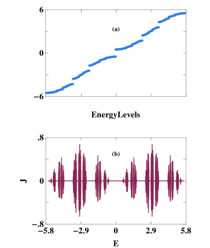
Figure 2: (Color online). (a) Energy levels and (b) $J$-$E$ characteristics of a $17$-th generation fibonacci ring when AB flux $\phi$ is set at $\phi_{0}/5$.

If we zoom any band in Fig. 2(b), it resembles the original spectrum since all the energy levels contribute to the current density. The major advantage of the RSRG approach is that it enormously reduces the computational load and enhances numerical accuracy in the calculation of persistent current of large systems like circular DNA. In the case of the $17$-th generation fibonacci ladder ring we have $2\times 1597$, i.e., $3194$ sites. The evaluation of persistent current needs Green’s functions, the determination of which requires the inversion of $3194\times 3194$ matrices. However, our present approach based on RSRG arguments makes the task very simple. We can determine this current simply from an effective $4$-th generation fibonacci ladder ring, the smallest possible fibonacci ring consisting of $6$ ($=2\times 3$) renormalized sites only.

It is now pertinent to raise a question whether persistent current calculated by this method agrees with the other existing methods gefen ; san1 ; san3 ; san4 or not. In order to address this question we have calculated persistent current using Eq. 18 and in Fig. 3 we present the current-flux ($I$-$\phi$) characteristics for a $10$-th generation fibonacci ladder ring considering $v=-0.5$ and setting the other parameters values identical to those used in Fig. 2. We have

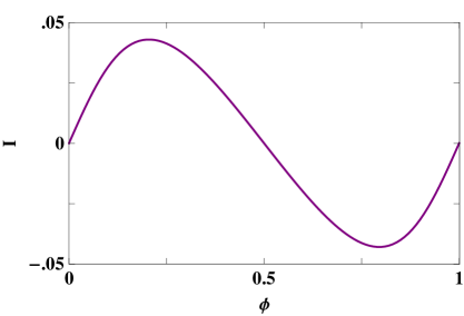
Figure 3: (Color online). Current-flux characteristics for a $10$-th generation fibonacci ring when $v=-0.5$ and $\mu=-2.1$.

checked that the $I$-$\phi$ curve matches very well with those obtained from the existing methods. To recover the on-site model for the fibonacci lattice from the general one, the parameters are needed to be chosen in the following manner: $\epsilon_{\alpha}=\epsilon_{\gamma}\neq\epsilon_{\beta}$, $t_{L}=t_{S}$ and $a_{L}=a_{S}$. Although in the present manuscript we have confined ourselves only to the fibonacci lattice, this method is quite general and readily applicable to ordered ($\epsilon_{\alpha}=\epsilon_{\gamma}=\epsilon_{\beta}$ and $t_{L}=t_{S}$) as well as other quasiperiodic, e.g. copper-mean, silver-mean, etc., lattices.

To conclude, in the present communication we have introduced a method relying on the RSRG approach to evaluate persistent current of a multi-channel fibonacci ring threaded by a magnetic flux. The key idea is based on the concept of the DOPC such that persistent current becomes an integral of it over energy. Within the TB framework we have expressed DOPC in terms of the Green’s functions of the system. The merit of the present scheme relies on the fact that one can reduce a higher generation fibonacci ring to an effective smallest possible fibonacci ring simply iterating a set of recursion relations (Eq. 16) for the system parameters and the task of finding DOPC of the original ring essentially reduces to that of the effective ring. Hence, the present method is computationally very efficient and gives persistent current of large system sizes with high accuracy. This approach is quite general since it is applicable to any periodic or quasiperiodic system, and has great potential when the system size is very large. The finite temperature extension of this formalism is also extremely trivial, one has to multiply the integral in Eq. 18 just by the Fermi factor and replace the upper limit by infinity.

References

- (1) L. P. Levy, G. Dolan, J. Dunsmuir, and H. Bouchiat, Phys. Rev. Lett. 64, 2074 (1990).
- (2) M. Büttiker, Y. Imry, and R. Landauer, Phys. Lett. A 96, 365 (1983).
- (3) A. L. Yeyati and M. Büttiker, Phys. Rev. B 52, R14360 (1995).
- (4) H. F. Cheung, Y. Gefen, E. K. Riedel, and W. H. Shih, Phys. Rev. B 37, 6050 (1988).
- (5) S. K. Maiti, J. Appl. Phys. 110, 064306 (2011).
- (6) P. Dutta, S. K. Maiti, and S. N. Karmakar, Eur. Phys. J. B 85, 126 (2012).
- (7) S. K. Maiti, J. Chowdhury, and S. N. Karmakar, J. Phys.: Condens. Matter 18, 5349 (2006).
- (8) S. K. Maiti, J. Chowdhury, and S. N. Karmakar, Phys. Lett. A 332, 497 (2004).
- (9) R. Deblock, R. Bel, B. Reulet, H. Bouchiat, and D. Mailly, Phys. Rev. Lett. 89, 206803 (2002).
- (10) B. Reulet, M. Ramin, H. Bouchiat, and D. Mailly, Phys. Rev. Lett. 75, 124 (1995).
- (11) D. Mailly, C. Chapelier, and A. Benoit, Phys. Rev. Lett. 70, 2020 (1993).
- (12) H. Bluhm, N. C. Koshnick, J. A. Bert, M. E. Huber, and K. A. Moler, Phys. Rev. Lett. 102, 136802 (2009).
- (13) S. Nakamae, M. Cazayous, A. Sacuto, P. Monod, and H. Bouchiat, Phys. Rev. Lett. 94, 248102 (2005).
- (14) S. Kim, J. Yi, and M. Y. Choi, Phys. Rev. E 76, 012902 (2007).
- (15) A.-M. Guo, H. Xu, Physica B 391, 292 (2007).
- (16) E. Maciá, J. Crystallogr. 224, 91 (2009).
- (17) E. Díaz, A. Sedrakyan, D. Sedrakyan, and F. Domínguez-Adame, Phys. Rev. B 75, 014201 (2007).
- (18) E. Maciá, Phys. Rev. B 74, 245105 (2006).
- (19) E. Maciá, Appl. Phys. Lett. 73, 3330 (1998).
- (20) D. Shechtman, I. Blech, D. Gratias, and J. W. Cahn, Phys. Rev. Lett. 53, 1951 (1984).
- (21) A. Chakrabarti, S. N. Karmakar, and R. K. Moitra, Phys. Rev. B 39, 9730(R) (1989).
- (22) M. Kohmoto, L. P. Kadanoff, and C. Tang, Phys. Rev. Lett. 50, 1870 (1983).
- (23) M. Kohmoto, B. Sutherland, and C. Tang, Phys. Rev.B 35, 1020 (1987).
- (24) S. Sil, S. N. Karmakar, R. K. Moitra, and A. Chakrabarti, Phys. Rev. B 48, 4192(R) (1993).
- (25) A. Ghosh and S. N. Karmakar, Phys. Rev. B. 58, 2586 (1998).
- (26) S. N. Karmakar, A. Chakrabarti, and R. K. Moitra, Phys. Rev. B 46, 3660 (1992).
- (27) A. Chakrabarti and S. N. Karmakar, Phys. Rev. B 44, 896(R) (1991).
- (28) J. P. Lu, T. Odagaki, and J. L. Birman, Phys. Rev. B 33, 4809, (1986).
- (29) G. J. Jin, Z. D. Wang, A. Hu, and S. S. Jiang, Phys. Rev. B 55, 9302 (1997).
- (30) X. F. Hu, R. W. Peng, L. S. Cao, X. Q. Huang, M. Wang, A. Hu, and S. S. Jiang, J. Appl. Phys. 97, 10B308 (2005).
- (31) Y. K. Vekilov, I. A. Gordeev, and E. I. Isaev, J. Exp. Theo. Phys. 89, 995 (1999).