Towards an Efficient Use of the BLAS Library for Multilinear Tensor Contractions

Abstract

Mathematical operators whose transformation rules constitute the building blocks of a multi-linear algebra are widely used in physics and engineering applications where they are very often represented as tensors. In the last century, thanks to the advances in tensor calculus, it was possible to uncover new research fields and make remarkable progress in the existing ones, from electromagnetism to the dynamics of fluids and from the mechanics of rigid bodies to quantum mechanics of many atoms. By now, the formal mathematical and geometrical properties of tensors are well defined and understood; conversely, in the context of scientific and high-performance computing, many tensor-related problems are still open. In this paper, we address the problem of efficiently computing contractions among two tensors of arbitrary dimension by using kernels from the highly optimized BLAS library. In particular, we establish precise conditions to determine if and when GEMM, the kernel for matrix products, can be used. Such conditions take into consideration both the nature of the operation and the storage scheme of the tensors, and induce a classification of the contractions into three groups. For each group, we provide a recipe to guide the users towards the most effective use of BLAS.

1 Introduction

In the last decade, progress in many scientific disciplines like Quantum Chemistry [1] and General Relativity [2] was based on the ability of simulating increasingly large physical systems. Very often, the simulation codes rely on the contraction of matrices and tensors [3]; surprisingly, while matrix operations are supported by numerous highly optimized libraries, the domain of tensors is still sparsely populated. In fact, the contrast is staggering: On the one hand, GEMM—the matrix-matrix multiplication kernel from the BLAS library—is possibly the most optimized and used routine in scientific computing; on the other hand, high-performance black-box libraries for high dimensional contractions are only recently starting to appear. This paper attempts to fill the gap, not by developing an actual tensor library—a “tensor-BLAS”—but by identifying when and how contractions among tensors of arbitrary dimension can be expressed, and therefore computed, in terms of the existing highly-efficient BLAS kernels.

Since the introduction of BLAS 1 in the early 70s’ [7], the numerical linear algebra community has made tremendous progress in the generation of high-performance libraries. Nowadays BLAS consists of three levels, corresponding to routines for vector-vector, matrix-vector and matrix-matrix operations [8, 9]. From a mathematical perspective, it might appear that this structure introduces unnecessary duplication: For instance, a matrix-matrix multiplication (a level 3 routine) can be expressed in terms of matrix-vector products (level 2), which in turn can be expressed in terms of inner products (level 1). Beyond convenience, the layered structure is motivated by the efficiency of the routines: Due to the increasing ratio between operation count and number of memory accesses—about 1/2, 2 and $n$/2 for BLAS 1, 2, and 3, respectively—, higher-level operations offer better opportunity to amortize the costly memory accesses with calculations. In practice, this means that level 3 routines attain the best performance and should be preferred whenever possible.

Intuitively, one would expect the ratio between flop count and memory accesses to continue growing with the dimension of the tensors involved in the contraction, suggesting a level 4 BLAS and beyond. While it might be worthwhile to further explore this research idea, since the potential of today’s processors is already fully exploited by BLAS 3 kernels, we aim at expressing arbitrary contractions in terms of those kernels.

Our study deals with contractions of any order between two tensors of arbitrary dimension; the objective is to provide computational scientists with clear directives to make the most out of the BLAS library, thus attaining near-to-perfect efficiency.

This paper makes two main contributions. First, it contains a set of requirements to quickly determine if and how a given contraction can be computed utilizing GEMM, the best performing BLAS kernel. These requirements lead to a 3-way classification of the contractions between two generic tensors. The second contribution consists of guidelines, given in the form of recipes, to achieve an optimal use of BLAS for each of the three classes, even when GEMM is not directly usable. In some cases, the use of BLAS 3 is only feasible in combination with copying operations, effectively equivalent to a transposition; in such cases, our guidelines indicate how the tensors should be generated so that the transposition is altogether avoided. To support our claims, we performed a number of experiments with contractions that arise frequently in actual applications; in all cases, our guidelines are confirmed by the observations. Furthermore, since our analysis of contractions from actual applications provides examples of operations that arise frequently and that are not currently supported by BLAS, we believe that this study will be helpful to library developers who wish to support tensor operations.

Related work

In recent years, the problem of efficiently handling tensor operations has been increasingly studied. A multitude of methods were proposed to construct low dimensional approximations to tensors. This research direction is very active, and orthogonal to the techniques discussed in this paper; we refer the reader to [4] for a review, and to [5, 6] for other advances. Two projects focus specifically on the computation of contractions: the Tensor Contraction Engine (TCE) and Cyclops [19, 18]. TCE offers a domain-specific language to specify multi-index contractions among two or more tensors; through compiler techniques it then returns optimized Fortran code under given memory constraints [20, 21]. Cyclops is instead a library for distributed memory architectures that targets high dimensional tensors arising in quantum chemistry [17]; high-performance is attained thanks to a communication-optimal algorithm, and cyclic decomposition for symmetric tensors. We stress that the approach described in this paper goes in a different direction, targeting dense tensors, and decomposing the contractions in terms of standard matrix kernels.

Organization of the paper

The paper is organized as follows. In Sec. 2, we introduce definitions, illustrate our methodology through a basic example, and present the tools and notation used in the rest of the paper. Section 3 constitutes the core of the paper: It contains the requirements for the use of GEMM, the classification of contractions, and recipes for each of the contraction classes. Next, in Sec. 4 we present a series of examples with performance results. Concluding remarks and future work are discussed in Sec. 5.

2 Preliminaries

We start with a list of definitions for acronyms and concepts used throughout the paper. We then illustrate our approach by means of a simple example in which the concept of “slicing” is introduced. Once a formal definition of algebraic tensor operations is given, we conclude by showing how slicing is applicable to contractions between arbitrary tensors.

2.1 BLAS definitions and properties

The main motivations behind the Basic Linear Algebra Subroutines were modularity, efficiency, and portability through standardization [10]. With the advent of architectures with a hierarchical memory, BLAS was extended with its levels 2 and 3, raising the granularity level to allow an efficient use of the memory hierarchy—by amortizing the costly data movement with the calculation of a larger number of floating point operations. With respect to the full potential of a processor, the efficiency of BLAS 1, 2, and 3 routines is roughly 5%, 20% and 90+%, respectively. It is widely accepted that for large enough operands, these values are nearly perfect. Moreover, the scalability of BLAS 1 and 2 kernels is rather limited, while that of BLAS 3 is typically close to perfect. As demonstrated by its universal usage, BLAS succeeded in providing a portability layer between the computing architecture and both numerical libraries and simulation codes.

In addition to the reference library, nowadays many implementations of BLAS exist, including hand-tuned [12, 11], automatically-tuned [23, 24], and versions developed by processors manufacturers [13, 15, 14]. Despite their excellent efficiency, such libraries might not be well suited for tensor computations. For instance, in the following it will become apparent that the design of the BLAS interface falls short when matrices are originated by slicing higher dimensional objects; specifically, costly transpositions are caused by the constraint that matrices have to be stored so that one of the dimensions is contiguous in memory. Recent efforts aim at lifting some of these shortcomings [25].

A list of BLAS related definitions follows.

• Stride: distance in memory between two adjacent elements of a vector or a matrix. BLAS requires matrices to be stored by columns, that is, with vertical $stride=1$.

• Leading dimension: distance between two adjacent row-elements in a matrix stored by columns. In BLAS routines, leading dimensions are specified through arguments.

• GEMM: $C\leftarrow\alpha A^{\bullet}B^{\bullet}+\beta C$; kernel for general matrix-matrix multiplication (BLAS 3). $A,B$ and $C$ are matrices; $\alpha$ and $\beta$ are scalars; $M^{\bullet}$ indicates that matrix $M$ can be used with/without transposition.

• GEMV: $y\leftarrow\alpha A^{\bullet}x+\beta y$; kernel for general matrix-vector multiplication (BLAS 2). $A$ is a matrix, $x$ and $y$ are vectors, and $\alpha$ and $\beta$ are scalars; $A^{\bullet}$ indicates that matrix $A$ can be used with/without transposition.

• GER: $C\leftarrow\alpha xy^{H}+C$; outer product (BLAS 2). $C$ is a matrix, $x$ and $y$ are vectors, and $\alpha$ is a scalar.

• DOT: $\alpha\leftarrow x^{H}y$; inner product (BLAS 1). $x$ and $y$ are vectors, and $\alpha$ is a scalar.

2.2 A first example

In order to illustrate our methodology with a first well-known example, and thus facilitate the following discussion, here we consider one of the most basic contractions, the multiplication of matrices.

To the reader familiar with the jargon based on Einstein convention, given two 2-dimensional tensors $A^{ih}$ and $B_{hj}$, we want to contract the $h$ index. In linear algebra terms, the matrices $A$ and $B$ have to be multiplied together.

$$C^{i}_{j}:=A^{ih}B_{hj},\text{ \quad or equivalently: \quad}c_{ij}:=\sum_{h}a_{ih}b_{hj},\ \forall i\forall j$$

For the sake of this example, we assume that only level 1 and 2 BLAS are available, while level 3 is not; in other words, we assume that there exists no routine that takes (pointers to) $A$ and $B$ as input, and directly returns the matrix $C$ as output. Therefore, we decompose the operation in terms of level 1 and 2 kernels by slicing the operands, exactly the same way we will later decompose a contraction between tensors in terms of matrix-matrix multiplications.

In the following, we provide a number of alternatives for slicing the matrix product. Matrices $A,B$ and $C$ are of size $m\times k$, $k\times n$, and $m\times n$, respectively. Also, $F^{i}$ and $F_{j}$ respectively denote the $i$-th row and $j$-th column of the matrix $F$.

1. $A$ is sliced horizontally. The slicing of $i$, the first index of $A$, leads to a decomposition of $C$ as a sequence of independent GEMVs: $C:=\forall_{i}\ a^{i}B$

   $$C:=AB=\left[\begin{array}[]{c}a^{1}\\ \hline\cr\vdots\\ \hline\cr a^{m}\end{array}\right]B=\left[\begin{array}[]{c}a^{1}B\\ \hline\cr\vdots\\ \hline\cr a^{m}B\end{array}\right].$$

2. $B$ is sliced vertically. The slicing of $j$, the second index of $B$, also leads to a decomposition of $C$ as a sequence of independent GEMVs: $C:=\forall_{j}\ Ab_{j}$

   $$C:=AB=A[b_{1}|b_{2}|\dots|b_{n}]=[Ab_{1}|Ab_{2}|\dots|Ab_{n}].$$

3. $A$ is sliced vertically and $B$ horizontally. The slicing of $h$, the contracted index, leads to expressing $C$ as a sum of GERs: $C:=\sum_{h}a_{h}b^{h}$

   $$C:=AB=[a_{1}|\dots|a_{k}]\left[\begin{array}[]{c}b^{1}\\ \hline\cr\vdots\\ \hline\cr b^{k}\end{array}\right]=a_{1}b^{1}+a_{2}b^{2}+\dots+a_{k}b^{k}.$$

4. $A$ is sliced horizontally and $B$ vertically. If both indices $i$ and $j$ are sliced, $C$ is decomposed as a two-dimensional sequence of DOTs: $C:=\forall_{i}\forall_{j}\ a^{i}b_{j}$

   $$C:=AB=\left[\begin{array}[]{c}a^{1}\\ \hline\cr\vdots\\ \hline\cr a^{m}\end{array}\right][b_{1}|\dots|b_{n}]=\left[\begin{array}[]{c | c | c}a^{1}b_{1}&\dots&a^{1}b_{n}\\ \hline\cr\vdots&\ddots&\\ \hline\cr a^{m}b_{1}&&a^{m}b_{n}\end{array}\right].$$

While mathematically these four expressions compute exactly the same matrix product, in terms of performance they might differ substantially. From this perspective, slicings 1–3 lead to level 2 BLAS kernels (GEMVs for 1 and 2, GERs for 3) and are thus to be preferred to slicing 4, which instead leads to level 1 kernels (DOT). In the following sections we will follow the same procedure for higher-dimensional tensors and multiple contractions.

2.3 Tensors definitions and properties

Due to their high-dimensionality, tensors are usually presented together with their indices. As commonly done in physics related literature, in the rest of the paper we use greek letters to denote indices. We now illustrate some concepts which are not strictly necessary to understand the methodology introduced in the following sections, but that are important to establish a connection with the language commonly used by physicists and chemists.

As explained in Appendix A, there is a substantial difference between upper (contravariant) and lower (covariant) indices. In general, the connection between covariant and contravariant indices is given by a special tensor $g_{\mu\nu}$ called “metric”. For example, an upper index of a vector $x$ can be lowered by multiplying the vector with the metric tensor (in itself having properties similar to those of a symmetric matrix):

$$x_{\mu^{\prime}}=\sum_{\mu=1}^{N}x^{\mu}g_{\mu\mu^{\prime}}\equiv x^{\mu}g_{\mu\mu^{\prime}}.$$

Notice that the right hand side is written without explicit reference to the sum over the $\mu$ index. This convention is usually known as the “Einstein notation”: Repeated indices come in couples (one upper and one lower index) and are summed over their entire range. We refer to this operation as a “contraction”. It is important to keep in mind that contractions happen only between equal indices lying on opposite positions. Following this simple rule, matrix-vector multiplication is written as

$$Ax\equiv A^{\alpha\beta}g_{\beta\gamma}x^{\gamma}\equiv A\indices{{}^{\alpha}_{\gamma}}x^{\gamma}.$$

Since a tensor can have more than one upper or lower index, we interpret lower indices as generalized “column modes” and the upper indices as generalized “row modes”. In general, it is common to refer to a $k$-dimensional tensor having $i$ row modes and $j$ column modes (with $i+j=k$) as a ($i,j$)-tensor or an “order-$k$ tensor”. Finally, since relative order among indices is important, the position of an index should be always accounted for; this is of particular importance in light of the results we present.

Having established the basic notations and conventions (see Appendix A for more details), we are ready to study numerical multilinear operations between tensors. We begin by looking at an example where only one index ($\gamma$) is contracted. In the language of linear algebra, the operation can be described as an inner product between a (3,0)-tensor and a (2,0)-tensor

$$R\indices{{}^{\alpha\beta\rho}}:=(T\indices{{}^{\alpha\beta\gamma}})\cdot(S^{\gamma\rho}).$$ (1)

In accordance with the convention, the summation over $\gamma$ can only take place once the index is lowered in one of the two tensors. For example, $\gamma$ can be lowered in $T$ as

$$T\indices{{}^{\alpha\beta\gamma}}\longrightarrow T\indices{{}^{\alpha\beta\mu}}g_{\mu\gamma}\equiv T\indices{{}^{\alpha\beta}_{\gamma}}.$$ (2)

The inner product (1) can then be written as a left multiplication of the last column-mode of $T$ with the first row-mode of $S$. Since $\gamma$ could have been lowered in $S$ (instead of $T$), mathematically this operation is exactly equal to a right multiplication between the last row-mode of $T$ and the first column-mode of $S$

$$T\indices{{}^{\alpha\beta}_{\gamma}}S^{\gamma\rho}\equiv T^{\alpha\beta\gamma}S\indices{{}_{\gamma}^{\rho}}.$$ (3)

The inner product (3) constitutes only one way of contracting one index of $T$ with one of $S$. In general, depending on which index is contracted, there are six mathematically distinct cases:

$$\begin{array}[c]{lllll}{\rm(i)}&T\indices{{}^{\alpha\beta}_{\sigma}}\;S^{\sigma\rho}=T\indices{{}^{\alpha\beta\gamma}}\ g_{\gamma\sigma}\ S^{\sigma\rho}&&{\rm(ii)}&T\indices{{}^{\alpha\beta}_{\rho}}\;S^{\sigma\rho}=T\indices{{}^{\alpha\beta\gamma}}\ g_{\gamma\rho}\ S^{\sigma\rho}\\[4.0pt] {\rm(iii)}&T\indices{{}^{\alpha}_{\sigma}{}^{\gamma}}\;S^{\sigma\rho}=T\indices{{}^{\alpha\beta\gamma}}\ g_{\beta\sigma}\ S^{\sigma\rho}&&{\rm(iv)}&T\indices{{}^{\alpha}_{\rho}{}^{\gamma}}\;S^{\sigma\rho}=T\indices{{}^{\alpha\beta\gamma}}\ g_{\beta\rho}\ S^{\sigma\rho}\\[4.0pt] {\rm(v)}&T\indices{{}_{\sigma}^{\beta\gamma}}\;S^{\sigma\rho}=T\indices{{}^{\alpha\beta\gamma}}\ g_{\alpha\sigma}\ S^{\sigma\rho}&&{\rm(vi)}&T\indices{{}_{\rho}^{\beta\gamma}}\;S^{\sigma\rho}=T\indices{{}^{\alpha\beta\gamma}}\ g_{\alpha\rho}\ S^{\sigma\rho}.\end{array}$$ (4)

Since the index sizes can differ substantially, the distinction among all these cases is not just formal. Additionally, a tensor can be symmetric with respect to the interchange of the first and third index but not with respect to the interchange between the first and the second. Consequently the mutual ordering among indices is quite important prompting to distinguish among cases with different ordering. Thus not only matters which index is contracted, but also in which position each index is. Ultimately, a tensor is a numerical object stored in the physical memory of a computer. We will see that index structure and storage strategies play a fundamental role in the optimal use of the BLAS library.

2.4 Slicing the modes

Here we discuss how the procedure used in Sec. (2.2) to slice matrices can be generalized to tensors, to produce objects manageable by BLAS. In general, an N-dimensional tensor is sliced by (N-1)-dimensional objects, and every slice is itself a tensor. Notice that the slicing language shifts the focus from the parts of the partitioned tensor to the partitioning object itself. As we will see in the next section, this shift in focus is at the core of our analysis.

To allow an easy visualization, let us again consider the contraction case (i) of Eq. (4). In order to reduce this operation to a sequence of matrix-matrix multiplications, the (2,1)-tensor $T\indices{{}^{\alpha\beta}_{\sigma}}$ needs to be sliced by a 2-dimensional object; such a slicing can be realized in several ways. For the sake of simplicity, let us represent $T$ as a 3-dimensional cube, and consider its slicing by one or more planes. Figure 1 shows three (out of seven) possible slicings of $T$ by different choices of planes.

Figure 1: Three possible slicing choices

• The cube is sliced by a plane defined by the modes $\alpha$ and $\sigma$.

• The cube is sliced by a plane defined by the modes $\beta$ and $\sigma$.

• This double slicing is defined by combining the two previous slicing, (a) and (b).

A simple yet effective way of describing the slicing of a tensor is by means of a vector $\vec{s}$ that indicates the indices that are sliced:

$$\vec{s}(T)=(s_{\alpha},s_{\beta},s_{\sigma}).$$ (5)

In this language, the previous three cases correspond to

• $\vec{s}_{a}(T)=(s_{\alpha},s_{\beta},s_{\sigma})=$ (0, 1, 0);

• $\vec{s}_{b}(T)=$ (1, 0, 0);

• $\vec{s}_{c}(T)=$ (1, 1, 0); this is the sum of the previous two slicings, $\vec{s}_{a}(T)+\vec{s}_{b}(T)=\vec{s}_{c}(T)$.

In the first case, $s_{\beta}=1$ means that the index $\beta$ is decomposed in a sequence of as many slices as the range of $\beta$. Accordingly, $s_{\alpha}$ and $s_{\sigma}$ take value 0, i.e., the slicing is made by planes defined by the modes $\alpha$ and $\sigma$ along the $\beta$ direction. Note that any combination of slicings results in an object of dimensionality $N-\|\vec{s}(T)\|_{1}$. For instance, slicing (c) produces a set of $3-2=1$-dimensional objects.

We now relate the slicing to mappings onto BLAS routines. To this end, we have to specify how the tensors are stored in memory. In the rest of the paper we always assume the first index of each tensor to have $stride=1$. The same way in Sec. 2.2 we decomposed the contraction between $A$ and $B$, in the following we decompose the contraction $R\indices{{}^{\alpha\beta\rho}}:=T\indices{{}^{\alpha\beta}_{\sigma}}\;S^{\sigma\rho}$ in three different ways. Here the tensors $T$, $S$ and $R$ are of size $m\times n\times k$, $k\times\ell$, and $m\times n\times\ell$, respectively. (Then the slices $R^{\alpha i\rho}$ are of size $m\times\ell$, and $T\indices{{}^{\alpha i}_{\sigma}}$ are of size $m\times k$.)

• $\vec{s}_{a}(T)=$ (0, 1, 0) leads to a sequence of matrix products directly mappable onto GEMMs since the dimensions with stride=1 remain unsliced: $R=\forall_{i}\ T_{i}S$.

• $\vec{s}_{b}(T)=$ (1, 0, 0) also leads to a sequence of matrix products; in this case, however, to enable the use of GEMM, each slice of $T$ must be copied on a separate memory region: $R=\forall_{i}\ (T_{i})_{cp}\ S$.

• $\vec{s}_{c}(T)=$ (1, 1, 0) leads to a sequence of GEMVs: $R=\forall_{i}\forall_{j}\ T_{ij}S$.
  

Once again, these three slicings lead to mathematically equivalent algorithms for computing the tensor $R$. In terms of performance, (a) is to be preferred, as it directly maps onto matrix products. Although slicing (b) also reduces the problem to a sequence of matrix-matrix products, since the slices have both dimensions with stride $>1$, these cannot be directly mapped onto GEMM; this means that a costly preliminary transposition is necessary. Finally, slicing (c) should be avoided, as it forms $R$ by means of matrix-vector products, thus relying on the slow BLAS 2 kernel.

3 The recipe for an efficient use of BLAS

Given two tensors of arbitrary dimension and one or more indices to be contracted, for performance reasons the objective is to map the calculations onto BLAS 3 kernels, and onto GEMM in particular. The mapping is obtained by slicing the tensors opportunely. Unfortunately, not every contraction can be expressed in terms of level 3 kernels, and even when that is possible, not every choice of slicing leads to the direct use of GEMM. In this section, we first show that by testing a small set of conditions it is possible to determine when and how GEMM can be employed. Then, according to these conditions, we classify the contractions in three groups, and for each group we provide a recipe on how to best utilize BLAS.

Ultimately, our tools are meant to help application scientists in two different scenarios. If they have direct control of the generation of the tensors, we indicate a clear strategy to store them so that the contractions can be performed avoiding costly memory operations. Conversely, if the storage scheme of the tensors is fixed, we give guidelines to use the full potential of BLAS.

3.1 Requirements to be satisfied for a BLAS 3 mapping

As illustrated in Sec. 2.4, a slicing transforms a contraction between two generic tensors $T$ and $S$ into a sequence (or a sum) of contractions between the slices of $T$ and those of $S$. To allow a mapping onto BLAS 3, both the slices of $S$ and $T$ need to conform to the GEMM interface (see Sec. 2.1). In the first place, they have to be matrices; hence $S$ and $T$ have to have at least $N=2$ indices, and if $N>2$, the tensor has to be sliced along $N-2$ of them. Moreover, the slices of $S$ and $T$ must have exactly one contracted and one free (non-contracted) index; in other words, we are looking for two-dimensional slices that share one dimension, the same way in the contraction $C:=AB$, the matrices $A\in\mathbf{R}^{m\times k}$ and $B\in\mathbf{R}^{k\times n}$ share the $k$-dimension, while $m$ and $n$ are free. Finally, the BLAS interface does not allow the use of matrices with stride $>1$ in both dimensions; therefore it is not possible to slice the indices of $S$ and $T$ that correspond to stride 1 modes without compromising the use of GEMM.

The previous considerations can be formalized as three requirements. Define $N(X)$ as the number of modes of tensor $X$, and let $R:=TS$ be a contraction.

• The modes of $T$ and $S$ with stride 1 must not be sliced.

• $T$ and $S$ have to be sliced along $N(T)-2$ and $N(S)-2$ modes, respectively. (In a compact language, $\|\vec{s}(T)\|_{1}=N(T)-2$ and $\|\vec{s}(S)\|_{1}=N(S)-2$). Notice that whenever a contracted index is sliced, both $T$ and $S$ are affected.

• The slices must have exactly one free and one contracted index. Therefore, it must be avoided to slice only all the contracted indices or only all the free ones.

Despite their simplicity, these three requirements apply universally to contractions $R=TS$ of any order between tensors of generic dimensionality. If they are all satisfied, then it is possible to compute $R$ via GEMMs; this is for instance the case of Example (a) in Sec. 2.4.

A precise classification of contractions is given in the next section. Let us now briefly discuss the scenarios in which exactly one of the requirements does not hold.

• If requirement R1 is not satisfied (the resulting slice does not have any mode with stride 1), the use of GEMM is still possible by copying each slice in a separate portion of memory. We refer to this operation as a COPY + GEMM, an example of whom is given by case (b) in Sec. 2.4.

• If $\|\vec{s}(T)\|_{1}>N(T)-2$ or $\|\vec{s}(S)\|_{1}>N(S)-2$, then it is not possible to use BLAS 3 subroutines; in this case, one has to rely on routines from level 2 or level 1, such as GEMV and GER, or even on no BLAS at all. An example is provided by case (c) in Sec. 2.4.

• As for F2, if all the contracted indices or all the free indices are sliced, one can use only BLAS 2, BLAS 1, or even no BLAS at all. An example is given by the contraction $R\indices{{}^{\alpha\beta\rho}}:=T\indices{{}^{\alpha\beta}_{\sigma}}\;S^{\sigma\rho}$ with $\vec{s}(T)=(0,0,1)$: the computation reduces to a sequence of element-wise operations.

3.2 Contraction classes

We now use the requirements for cataloging all contractions in a small set of classes; most importantly, for each class we provide a simple recipe, indicating how to achieve an optimal use of BLAS. The aim is to empower computational scientists with a precise and easy-to-implement tool: Ultimately, these recipes shed light on the importance of choosing the correct strategy for generating and storing tensors in memory.

Given two tensors $t_{1}$ and $t_{2}$, and the number of contractions $p$, let us define $\Delta(t_{i})$ as $N(t_{i})-p$, with $i=1,2$ ($\Delta$ counts the number of indices of $t_{i}$ minus the number of contracted indices, that is, the number of free indices). The following classification is entirely based on $\Delta(t_{1})$ and $\Delta(t_{2})$.

3.2.1 Class 1: $\Delta(t_{1})=0$ and $\Delta(t_{2})=0$

The tensors have the same number of modes and they are all contracted; this operation produces a scalar. For example,

$$\kappa:=T\indices{{}^{\alpha\beta\gamma}}S\indices{{}_{\alpha\beta\gamma}}.$$ (6)

This situation is rather uncommon, yet possible. It can be considered as an extreme example of F3 in which there are no free indices; GEMM is therefore not applicable. Moreover, since BLAS does not support operations with more than one contracted index, one is forced to slice $k-1$ indices, resulting in an element-wise product and a sum-reduction to a scalar. The only opportunity for BLAS lies in level 1. For instance, in Eq. (6) it is possible to slice the indices $\alpha$ and $\beta$, $\vec{s}(T)=(1,1,0)\equiv\vec{s}(S)=(1,1,0)$; in both tensors, the slices are thus vectors along $\gamma$, and participate in DOT operations.

RECIPE, Class 1.

Slice all but one index. Use DOT with the unsliced mode. Then sum-reduce the result of all DOT’s.

3.2.2 Class 2: $\Delta(t_{1})\geq 1$ and $\Delta(t_{2})=0$

This class contains all the contractions in which only one tensor has one or more free indices. Let us look for example at

$$R\indices{{}^{\mu_{1}\dots\mu_{n}}}:=T\indices{{}^{\mu_{1}\dots\mu_{n}\beta\gamma}}S_{\beta\gamma}.$$

Requirement R2 forces $T$ to be sliced $n$ times. Moreover, since BLAS allows at most one contracted index, $S$ still requires to be sliced along $N(S)-1$ indices, leading to a sequence of vectors. This means that there is no possible choice that allows the use of GEMM: At best, the contraction is computed via matrix-vector operations.

Motivated by Eq. (4), we use the next three double contractions as explanatory examples.

$$(1^{\prime})\ R^{\alpha}:=T\indices{{}^{\alpha\beta\gamma}}g_{\beta\gamma}\qquad(2^{\prime})\ R^{\gamma}:=T\indices{{}^{\alpha\beta\gamma}}g_{\alpha\beta}\qquad(3^{\prime})\ R^{\beta}:=T\indices{{}^{\alpha\beta\gamma}}g_{\alpha\gamma}.$$ (7)

In order to make use of BLAS routines, $T$ has to be sliced at least once. For the contraction ($1^{\prime}$), there are three possible choices:

• $\vec{s}(T)=(0,0,1)$, and consequently $\vec{s}(g)=(0,1)$. This option does not slice the stride 1 modes but falls under the case F2, thus only GEMV is available;

• $\vec{s}(T)=(0,1,0)$, and consequently $\vec{s}(g)=(1,0)$. This situation is completely analogous to the previous one.

• $\vec{s}(T)=(1,0,0)$ and $\vec{s}(g)=(0,0)$. Each slice of $T$ has all its indices contracted with those of $g$. Although the index with stride 1 is sliced (case F1), this example falls under the case F3, where we sliced the only free index of $T$. As a consequence, the use of BLAS is limited to DOT.

The analysis of contractions ($2^{\prime}$) and ($3^{\prime}$) goes along the same lines: both cases present a choice of slicing leading to a GEMV and a DOT. The only additional situation arises when $\vec{s}(T)=(1,0,0)$, and consequently $\vec{s}(g)=(1,0)$; this choice slices the index of $T$ which carries stride 1. Thus, it is not possible to use GEMV, unless each slice of $T$ is transposed; we refer to this operation as COPY + GEMV.

RECIPE, Class 2,

If the index of $t_{1}$ with stride 1 is contracted, then slice all the other contracted indices, and all the free indices but one. Vice versa, if the index of $t_{1}$ with stride 1 is free, then slice all the other free indices, and all the contracted indices but one. In all cases, the use of GEMV is possible. As a rule of thumb to maximize performance, keep the indices with largest size unsliced.

3.2.3 Class 3: $\Delta(t_{1})\geq 1$ and $\Delta(t_{2})\geq 1$

From a computational point of view, this is the most interesting class of contractions. Both tensors have free indices, and a mapping onto either GEMM or COPY + GEMM always exists. In fact, according to requirement R2, both tensors have two or more indices and can therefore be sliced into a series of matrices. Moreover, both tensors have at least a free index and at least a contracted index, also satisfying requirement R3.

To express these contractions as matrix-matrix products—but not necessarily as straight GEMMs—it suffices to slice the tensors so to create matrices with a single (shared) contracted index, and a free one. Whether requirement R1 is satisfied too—thus being able to use GEMM— or not, splits this class in two subclasses.

Class 3.1: The indices with stride 1 of $t_{1}$ and $t_{2}$ are distinct, and both are contracted. In order to satisfy requirement R3 (creating slices with one free and one contracted index), only one of these indices can be left untouched, while the other has to be sliced. This leads to two alternatives: a) proceed to use COPY + GEMM, and b) map onto BLAS 2 kernels.

Class 3.2: The indices with stride 1 of $t_{1}$ and $t_{2}$ are the same, or are distinct and only one of them is contracted. There is enough freedom to always avoid slicing the indices of stride 1 in both tensors, thus granting viable map(s) to GEMM.

To illustrate the differences between these two sub-classes, we discuss, as a test case, the double contractions between two 3-dimensional tensors, $A^{\alpha\beta\gamma}$ and $B_{\theta\eta\rho}$. In general, ignoring internal symmetries of the operands and assuming that all dimensions match, $A$ and $B$ can be contracted in 18 distinct ways. In Table 1 we divide the contractions in three groups: while the positions and the labels of the indices of $A$ are fixed, each group has a different combination of contracted indices with $B$. As for the previous examples, we assume that each operand is stored in memory so that its first index has stride 1.

Table 1: Double contractions between two 3-dimensional tensors

	$\Delta(A)=1$ and $\Delta(B)=1$
Free index in $B$	$\beta$ and $\gamma$ contracted		$\alpha$ and $\gamma$ contracted		$\alpha$ and $\beta$ contracted
3rd	$A^{\alpha\beta\gamma}B_{\beta\gamma\eta}$	$A^{\alpha\beta\gamma}B_{\gamma\beta\eta}$	$A^{\alpha\beta\gamma}B_{\alpha\gamma\eta}$	$\mathbf{A^{\alpha\beta\gamma}B_{\gamma\alpha\eta}}$	$A^{\alpha\beta\gamma}B_{\alpha\beta\eta}$	$A^{\alpha\beta\gamma}B_{\beta\alpha\eta}$
2nd	$A^{\alpha\beta\gamma}B_{\beta\eta\gamma}$	$A^{\alpha\beta\gamma}B_{\gamma\eta\beta}$	$A^{\alpha\beta\gamma}B_{\alpha\eta\gamma}$	$A^{\alpha\beta\gamma}B_{\gamma\eta\alpha}$	$A^{\alpha\beta\gamma}B_{\alpha\eta\beta}$	$A^{\alpha\beta\gamma}B_{\beta\eta\alpha}$
1st	$\mathbf{A^{\alpha\beta\gamma}B_{\eta\beta\gamma}}$	$A^{\alpha\beta\gamma}B_{\eta\gamma\beta}$	$A^{\alpha\beta\gamma}B_{\eta\alpha\gamma}$	$A^{\alpha\beta\gamma}B_{\eta\gamma\alpha}$	$A^{\alpha\beta\gamma}B_{\eta\alpha\beta}$	$A^{\alpha\beta\gamma}B_{\eta\beta\alpha}$

We analyze the two cases highlighted in the table; it will then become clear that the remaining 16 contractions belong to either Class 3.1 (12 cases) or Class 3.2 (4 cases). These same two cases will serve in the next section as a template for the numerical tests.

Figure 2: $R\indices{{}^{\beta}_{\eta}}:=A^{\alpha\beta\gamma}B_{\gamma\alpha\eta}$: The direct use of GEMM is not possible; different slicing choices lead to different kernels.

The first contraction, $R\indices{{}^{\beta}_{\eta}}:=A^{\alpha\beta\gamma}B_{\gamma\alpha\eta}$, belongs to Class 3.1; no choice of slicing allows the direct use of GEMM. By slicing the first index of one of the two tensors, i.e., either $\vec{s}(A)=(1,0,0)$ (and $\vec{s}(B)=(0,1,0)$), or as in Fig. 2(a), $\vec{s}(B)=(1,0,0)$ (and $\vec{s}(A)=(0,0,1)$), one ends up with COPY + GEMMs. Alternatively, either one or both tensors can be sliced twice; Figures 2(b) and (c) diplays two possible choices: the first one—$\vec{s}_{A}=(0,0,1)$ and $\vec{s}_{B}=(1,0,1)$—violates requirement R2 and leads to GEMVs, while the second one—$\vec{s}_{A}=(1,0,1)$ and $\vec{s}_{B}=(1,1,0)$—violates requirements R2 and R3, and produces GERs.

The second case, $R\indices{{}^{\beta}_{\eta}}:=A^{\alpha\beta\gamma}B_{\eta\beta\gamma}$, belongs to class 3.2, and is an example in which multiple choices of slicing equivalently result in GEMM. In fact, both $\vec{s}(A)=(0,1,0)$ (and consequently $\vec{s}(B)=(0,1,0)$), and $\vec{s}(A)=(0,0,1)$ (and consequently $\vec{s}(B)=(0,0,1)$) are valid slicings that lead to GEMM (see Fig. 3).

Figure 3: Two slicing choices for $R\indices{{}^{\alpha}_{\eta}}:=A^{\alpha\beta\gamma}B_{\eta\beta\gamma}$, both leading to GEMM.

For all the remaining 16 cases of Table 1, the same considerations hold: If $A$ and $B$ are stored so that their first indices are either not contracted, or contracted and the same, then GEMM can be used directly. Otherwise, one must pay the overhead due to copying of data (COPY + GEMM), or rely on less efficient lower level BLAS.

Finally, inspired by the contractions arising frequently in Quantum Chemistry and in General Relativity, we cover now one additional example that involves two tensors of order four. Instead of describing all the possible cases, we only present two double contractions between a (4,0)-tensor $X$ and a (2,2)-tensor $Y$, again corresponding to classes 3.1 and 3.2.

$$(a)\quad R^{\alpha\beta\gamma\delta}:=X^{i\alpha j\beta}Y\indices{{}_{i}^{\gamma}{}_{j}^{\delta}}\qquad\qquad\qquad(b)\quad R^{\alpha\beta\gamma\delta}:=X^{i\alpha j\beta}Y\indices{{}_{j}^{\gamma}{}_{i}^{\delta}}.$$ (8)

These contractions only differ for the relative position of the indices $i$ and $j$ in the tensor $Y$.

Case ($a$) admits more than one choice to perform GEMM. As an example, the slicing vectors $\vec{s}(X)=(0,0,1,1)$ and $\vec{s}(Y)=(0,0,1,1)$ satisfy all three requirements R1, R2, and R3. In case ($b$), due to the fact that both contracted indices $i$ and $j$ are the indices with stride 1, GEMM cannot be used directly. Here we list three possibilities, each one originating computation that matches a different BLAS routine.

• $\vec{s}(X)=(0,0,1,1)$ and $\vec{s}(Y)=(1,1,0,0)$ $\longrightarrow$ COPY + GEMM;
  In this case, we violate R1. Since the first index of $Y$ is sliced, the resulting matrices (identified by the values of $j$ and $\gamma$) do not have any dimension with stride 1. Consequently each slice has to be copied on a separate memory allocation before GEMM can be used.

• $\vec{s}(X)=(0,1,0,1)$ and $\vec{s}(Y)=(0,1,0,1)$ $\longrightarrow$ DOT;
  Instead of R1, here we violate R3. All the free indices of both tensors are sliced, forcing the double contraction to be computed simultaneously: This is equivalent to compute a series of inner products and sum over them.

• $\vec{s}(X)=(1,0,1,1)$ and $\vec{s}(Y)=(1,0,1,1)$ $\longrightarrow$ GER.
  Both R2 and R3 are violated. All contracted indices are sliced, and only two free indices (one for each tensor) are left untouched. This corresponds to a series of outer products to be summed over.

In Sec. 4.2, we use exactly these slicing choices to give an idea of the performance of these different routines in the case of (highly skewed) rectangular tensors.

RECIPE, Class 3.1.

The objective is to use COPY + GEMM. Therefore, for either $t_{1}$ or $t_{2}$, keep the first index untouched, and slice all the others contracted indices; for the other, slice all the contracted indices but one. In both tensors, slice all the free indices but one. In general, the best performance is attained when the dimension of largest size is left untouched; however, the actual efficiency depends on the actual BLAS implementation. If possible, avoid this class altogether by storing the tensor in memory so that the contraction falls in class 3.2

RECIPE, Class 3.2.

GEMM is always possible. Leave both the stride-1 indices untouched. Slice the other indices to satisfy requirements R2 and R3. For best performance, keep untouched the index with largest size.

3.3 BLAS and memory storage

Independently of the order of the tensors $t_{1}$ and $t_{2}$ and of the number of contractions, our classification by means of $\Delta(t_{i})$ is a general tool to easily determine whether GEMM is usable or not. For a given operation, the user can immediately determine the class to which it belongs. If both $\Delta(t_{1})$ and $\Delta(t_{2})$ equal 0, it is only possible to use DOT. If exactly one between $\Delta(t_{1})$ and $\Delta(t_{1})$ equals 0, then BLAS 2 operations are usable. Finally, the most interesting scenario is when both $\Delta(t_{1})$ and $\Delta(t_{2})$ are greater or equal to 1: In this case there is always the opportunity of using GEMM, provided the tensors can be generated or stored in memory suitably. In this respect, the recipes also provide guidelines on how tensors should be arranged for maximum performance.

If the user has no freedom in terms of generation and storage of the tensors, GEMM is still amenable, but at the cost of an overhead caused by copying and transposing. Whenever possible, this option should be avoided. Nonetheless, in general COPY + GEMM still performs better than BLAS 2 kernels; moreover, the transpositions can be optimized to reduce the number of memory accesses and therefore the total overhead. In the next section, we present the performance that one can expect for each of the classes.

4 Numerical experiments

In this section, we present two numerical studies involving double contractions. The experiments mirror the two examples analyzed in Sec. 3.2.3; the aim is to support our deduction-based assumptions on the use of BLAS 3, and give insights on which are the most convenient alternatives when the direct use of GEMM is ruled out.

In the first study, we look at 3-dimensional tensors with indices of equal size (square tensors), and measure the performance as function of the size for four different alternatives—GEMM, COPY + GEMM, GEMV, GER.

The second study is inspired by two common applications of tensorial algebraic calculations: Coupled-Cluster method (CCD) in Quantum Chemistry, and General Relativity on a lattice [20, 22]. In these applications, tensors are usually rectangular, with one of more order of magnitude of difference in the size of the indices. Our objective is to verify that imposing the requirements of Sec. 3.1 is still a valid option, even in extreme cases in which the efficiency of BLAS 2 kernels is comparable to that of GEMM

All the numerical tests were carried out on two different architectures: tesla, an 8-core machine based on the 2.00 GHz Intel Xeon E5405 processor equipped with 16GB of memory (theoretical peak performance of 64 GFLOPS), and peco, an 8-core machine based on the 2.27 GHz Intel Xeon E5520 processor equipped with 24GB of memory (theoretical peak performance 72.6 GFLOPS). In both platforms, we compiled with gcc (ver. 4.1.2) and used the OpenBLAS library (ver. 0.1) [16]; in all cases, double precision was used, and performance is reported in terms of floating points operations/second.

4.1 3-dimensional square tensors with $\Delta(t_{i})=1$

We consider the contractions $R\indices{{}^{\alpha}_{\eta}}:=A^{\alpha\beta\gamma}B_{\eta\beta\gamma}$ and $R\indices{{}^{\beta}_{\eta}}:=A^{\alpha\beta\gamma}B_{\gamma\alpha\eta}$, and the operations resulting from the slicings depicted in Fig. 2 and 3. Specifically, in Figg. 4 and 5 we show the execution times for the computation of $R$ when using GEMM (in two different ways), COPY + GEMM, GEMV, and GER.

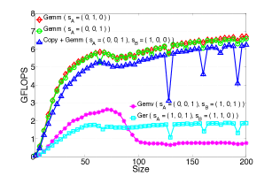
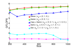
Figure 4: Performance (number of floating point operations executed per second) for the computation of $R\indices{{}^{\alpha}_{\eta}}:=A^{\alpha\beta\gamma}B_{\eta\beta\gamma}$ and $R\indices{{}^{\beta}_{\eta}}:=A^{\alpha\beta\gamma}B_{\gamma\alpha\eta}$ on 1 core of tesla.

As expected, the two slicings leading to GEMM outperform considerably those that instead make use of BLAS 2 routines. In fact, for tensors of size 150 and larger, each routine attains the efficiency level mentioned in the introduction: 90+% of the theoretical peak for GEMM, and between 10% to 20% of peak for BLAS 2 routines. This is an example of the clear benefits due to the use of BLAS-3 routines instead of those from BLAS 2 and 1. Additionally, the plots show that when COPY + GEMM is used, for tensors of size 200 or larger the overhead due to copying becomes apparent. In short, the results are in agreement with the discussion from Sec. 3.3: Whenever the contraction falls in the third class, the use of GEMM is preferable. If the dimensions are small, there is little difference between COPY + GEMM and GEMM; for mid and large sizes instead, it is always convenient to store the tensors so as to enable the direct use of GEMM, thus avoiding any overhead (class 3.2).

Figure 5 illustrates the results for a parallel execution on all the eight cores of tesla, using multi-threaded BLAS. It is not surprising to observe the increase of the gap between GEMM and BLAS 2 based routines. Moreover, comparing Fig. 4 and Fig. 5, one can also appreciate the larger performance gap between GEMM and COPY + GEMM, confirming the fact that on multi-threaded architectures it is even more crucial to carefully store the data to avoid unnecessary overheads. In fact, as explained in Sec. 3.3, the tensors with $\Delta(t_{i})\geq 1$ should be stored in memory so that the dimension with stride 1 is not one of the contracted indices; this choice prevents the use of COPY + GEMM and the consequent loss in performance. Finally, we point out that even though the two GEMM-based algorithms traverse the tensors in different ways, they attain the exact same efficiency.

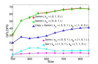
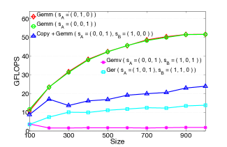
Figure 5: Performance in GFLOPS for the computation of $R\indices{{}^{\alpha}_{\eta}}:=A^{\alpha\beta\gamma}B_{\eta\beta\gamma}$ and $R\indices{{}^{\beta}_{\eta}}:=A^{\alpha\beta\gamma}B_{\gamma\alpha\eta}$ on 8 cores of peco(left) and tesla(right).

In conclusion, with this first example we confirmed that when performing double contractions on square tensors, any slicing that leads to GEMM  constitutes the most efficient choice, The situation does not change as the order of the tensors and the number of contracted indices increase.

4.2 4-dimensional rectangular tensors with $\Delta(t_{i})=2$

We shift the focus to real world scenarios in which the tensors are rectangular and possibly highly skewed. The objective is to test the validity of our recipes in situations, inspired by scientific applications, more general than contractions between square tensors. For this purpose, we concentrate on double contractions between 4-dimensional tensors. We present here two numerical examples: The first arises in the Coupled-Cluster method, while the second is motivated by covariant operations appearing in General Relativity. All these tests refer to the tensors $X$ and $Y$ presented in Sec. 3.2.3, and the slicings described for Eq. (8). In particular, $R^{\alpha\beta\gamma\delta}$ was computed via four algorithms (resulting from four different slicings), using GEMM, COPY + GEMM, DOT, and GER, respectively.

Example 1: Coupled-Cluster method.

For practical purposes, in Sec. 3.2.3 we introduced two different conventions for the tensor indices: We indicated the free and the contracted indices with letters from the Greek and Latin alphabet, respectively; when dealing with rectangular tensors, this notation is especially handy. In Quantum Chemistry, tensors indicate operators that allow the transition between occupied and virtual orbitals in a molecule. In the initial two examples, Greek indices correspond to occupied electronic orbitals, while Latin indices indicate unoccupied orbitals. Because of their physical meaning, the range of the indices $\alpha$, $\beta$, $\gamma$ and $\delta$ in Eq. (8) is quite different than that of $i$ and $j$. Normally, the former is a group of “short” indices (size $\in[30,\dots,100]$), while the latter are “long” indices (size $\in[1000,\dots,3000]$) [20].

One of the consequences of these typical index ranges is that $X$ and $Y$ can easily exceed the amount of main memory of standard multi-core computers. For example, if the indices $\alpha$, $\beta$, $\gamma$ and $\delta$ were all of size 80, and $i$ and $j$ were both of size 2000, the tensors $X$ and $Y$ would each require 204 GBs of RAM. In practice contractions with such large tensors are executed in parallel on clusters consisting of several computing nodes: $X$ and $Y$ are then distributed among the memory of many multi-core nodes avoiding altogether the issue of memory size.

In order to run numerical tests on just one multi-core node, we slightly reduced the size of the tensors, but kept the ratio between the size of the long and short indices unchanged. Moreover due to the heavy computational load, we fixed the free index $\beta$ to have value equal to one (see Figg. 6 and 7). Effectively, this is equivalent to computing one single slice of $R^{\alpha\beta\gamma\delta}$ as opposed to all of them; since $\beta$ is a free index, this simplification has no influence over the performance of the algorithms.

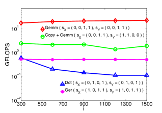
(a) Fixed $\alpha=\gamma=\delta=30$ and varying $i,j$

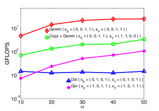
(b) Fixed $i=j=1,000$ and varying $\alpha,\gamma,\delta$

Figure 6: Performance (in GFLOPS, on a logarithmic scale) for the computation of $R^{\alpha\beta\gamma\delta}:=X^{i\alpha j\beta}Y\indices{{}_{i}^{\gamma}{}_{j}^{\delta}}$ on 8 cores of peco. On the left, the size of the indices $\alpha=\gamma=\delta$ is set to 30, while that of $i=j$ varies. On the right, the size of $i=j$ is set to 1000, while that of $\alpha=\gamma=\delta$ varies. In all cases, the free index $\beta$ is fixed.

The geometry of these tensors dictates that the 2-dimensional slices are not square matrices anymore. In fact, the slicings that lead to GEMM originate long and skinny matrices with an aspect ratio of about 100:1; on the contrary, those that lead to GER originate many short vectors. Figure 6 (in logarithmic scale) suggests that even in these cases, the algorithms based on GEMM are preferable to those that instead make use of lower levels of BLAS. Indeed, in basically all tests, GEMM is about one order of magnitude faster than COPY + GEMM, and almost two orders faster than GER and DOT.

Example 2: General relativity.

In this last set of experiments, we consider the scenario in which the contracted indices ($i,j$) are extremely short (size = 4), while the free indices are long (size $\leq$ 1,000). This scenario takes inspiration from a simplified version of 2-dimensional covariant tensors discretized on a 4-dimensional pseudo-euclidean lattice representing the space-time continuum. In order to make calculations and storage feasible, instead of working with 6-dimensional tensors, we only operate on a subset of the indices, maintaining the number of contractions unchanged. Due to its highly non-square aspect ratio, this example represents a rather extreme case that over-penalizes GEMM with respect to the other BLAS routines. In fact, while in the Coupled-Cluster example the matrices were multiplied via GEMM contracting their long side, here GEMM contracts the skinny matrices along their short side. The same scenario presents itself for the DOT case, where the contracted slices are made of short vectors. On the contrary, the slicings leading to GER end up in outer-multiplications of long vectors.

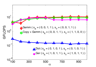
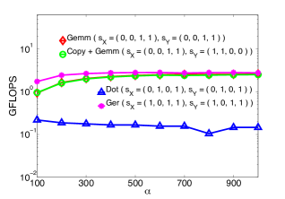
Figure 7: Performance (in GFLOPS, on a logarithmic scale) for the computation of $R^{\alpha\beta\gamma\delta}:=X^{i\alpha j\beta}Y\indices{{}_{i}^{\gamma}{}_{j}^{\delta}}$ on 8 cores of peco(left) and tesla(right). The size of the indices $i$ and $j$ is set to 4, while that of $\alpha=\gamma=\delta$ varies. The free index $\beta$ is fixed.

In Fig. 7 (in logarithmic scale), the performance of GEMM drops substantially, to the point that GEMM becomes comparable to both COPY + GEMM and GER. This sharp performance leveling is due to the extreme small size of the contracted index of the input matrix slices: While GER attains its peak performance due to the large size of the involved vectors, GEMM is rarely optimized for this specific shape (short contracted index). In the case of tesla, the GER-based contractions are, even if slightly, more efficient than GEMM. Although this result is somewhat expected, it shows that even in this example GEMM-based contractions are at least at the same level with the other BLAS sub-routines. DOT performance is once again lower than the other routines confirming that even in this extreme case it is always best to use higher levels of BLAS.

In conclusion, all the tests confirm the prominent role of GEMM for algebraic tensor operations and establish the necessity of adopting tensor storing practices that favor its use.

5 Conclusions

In this paper we look at multi-contractions between two tensors through the lens of the highly optimized BLAS libraries. Since the BLAS routines operate only with vectors and matrices, we illustrated a slicing technique that allows the structured reduction of each tensor into many lower dimensional objects. Combined with constraints of the BLAS interface, this technique naturally leads to the formulation of a set of requirements for the use of GEMM, the best performing BLAS routine. By using such requirements, we carried out a systematic analysis which resulted in a classification of tensor contractions in three classes. For each of these classes we provided practical guidelines for the best use of the available BLAS routines.

In the last section numerical experiments were performed with the aim of testing the validity of our guidelines with particular attention to real world scenarios. All examples confirm that for the optimal use of the BLAS library, particular care has to be placed in generating and storing the tensor operands. Specifically for contractions leaving at least one free index per tensor, the operands should be directly initialized and allocated in memory so as to avoid the index with stride 1 be the contracted one, and in doing so favor the direct use of GEMM.

Appendix

Appendix A Tensors on a manifold

The scientific community generically refers to multi-dimensional arrays as tensors, and uses this term in its most broadly defined sense. Sometimes such a fuzzy use of the term “tensor” may create confusion in the reader that is novel to this field. To avoid any confusion we will refer, in the following, to the mathematically rigorous definition of tensor used in differential geometry (sometimes also called tensor field). In this context a tensor is a mathematical object whose properties depend on the point of the geometrical manifold where it is defined. If such a manifold is a simple euclidean space provided with cartesian coordinates, a tensor is indistinguishable from a multi-dimensional array. On the contrary, adopting a more stringent tensor definition, allows to extend the results of this paper to the most general case of tensor fields.

The geometrical properties of a manifold $X$ are, in general, encoded in a symmetric and non-singular (admitting an inverse) two-index object $g_{\mu\nu}$ called “metric”. In a manifold there are two intrisically different objects that have the characteristics of a traditional vector: the vector proper $V^{\mu}$ and the dual vector $\omega_{\mu}$. A vector is changed into a dual vector by the metric

$$V_{\mu^{\prime}}=\sum_{\mu=1}^{N}V^{\mu}g_{\mu\mu^{\prime}}\equiv V^{\mu}g_{\mu\mu^{\prime}},$$

where the Einstein convention has been used in the last equality. Due to the uniqueness of the metric in defining the geometry of $X$, scalar products can only be computed among vectors once one of them is transformed into a dual vector by the metric

$$V^{\mu}\cdot W^{\nu}=V^{\mu}g_{\mu\nu}W^{\nu}\equiv V^{\mu}W_{\mu}\equiv V_{\nu}W^{\nu}.$$

This is what we refer to as “index contraction”.

The above expressions can be interpreted in the language of linear algebra if we think of a vector $V^{\mu}$ as a column n-tuple and a dual vector as a row n-tuple

$$V^{\mu}=\left(\begin{array}[]{l}V^{1}\\ \vdots\\ V^{n}\end{array}\right)\qquad;\qquad\omega_{\mu}=(\omega_{1}\dots\omega_{n})$$

Based on this analogy we can establish a notational language by imposing that

• any LOWER (covariant) index $\longrightarrow$ is a COLUMN index

• any UPPER (contravariant) index $\longrightarrow$ is a ROW index

So a general multi-indexed tensor with $M$ lower and $N$ upper indices $T\indices{{}^{\mu_{1}^{\prime}\dots\mu_{N}^{\prime}}_{\nu_{1}^{\prime}\dots\nu_{M}^{\prime}}}$ can be thought as a multi-array object having

• M covariant indices corresponding to M column-modes

• N contravariant indices corresponding to N row-modes.

If with $g_{\mu\nu}$ one can lower the indices of a generic tensor, the inverse of the metric $g^{\mu\nu}$ is used to raise tensor indices. In other words the metric transforms a row index in a column index while the inverse of the metric accomplishes the opposite. For example

$$T\indices{{}^{\alpha\beta\gamma}_{\rho\sigma\tau}}g_{\beta\nu}= T\indices{{}^{\alpha}_{\nu}{}^{\gamma}_{\rho\sigma\tau}}$$

$$T\indices{{}^{\alpha\beta\gamma}_{\rho\sigma\tau}}g^{\sigma\mu}= T\indices{{}^{\alpha\beta\gamma}_{\rho}{}^{\mu}_{\tau}}$$

From these examples we can infer the following:

• lowering is equivalent to row-mode multiplication with any (since $g$ is symmetric) column mode of the metric;

• raising is equivalent to column-mode multiplication with any row-mode of $g$.

Having defined the basic rules and language, we can now define a generic multiple contraction between two tensors

$$T\indices{{}^{\alpha\beta\gamma}_{\rho\sigma\tau}}g_{\beta\eta}g^{\sigma\xi}S\indices{{}^{\mu\eta}_{\xi\nu}}=T\indices{{}^{\alpha\beta\gamma}_{\rho\sigma\tau}}S\indices{{}^{\mu}_{\beta}{}^{\sigma}_{\nu}}=R\indices{{}^{\alpha\mu\gamma}_{\rho\beta\tau\nu}}.$$

In other words a contraction between two tensors $T$ and $S$ requires:

• two indices carrying the same symbol (repeated indices), one on $T$ and one on $S$;

• one of the two repeated indices has to be a row mode while the other has to necessarily be a column mode;

• each lowering and rising operation is performed by a metric tensor.

As for matrices, a tensor can be characterized by explicitly indicating its indices as well as their respective order. With these convention, a common matrix is a 2-tensor in a cartesian euclidean space. A general 2-tensor is not a matrix though, and matrix-matrix multiplications depend strictly on the geometry of the manifold where such 2-tensor live. In euclidean space with a cartesian coordinate system, the metric is just the identity but already if the space is equipped with spherical coordinates this is not true anymore

For instance, if we want to describe $\mathbb{R}^{3}-\{0\}$ in spherical coordinates it is necessary to make the following change of coordinates

$$\left(x,y,z\right)\overset{f}{\longrightarrow}\left(r,\theta,\phi\right):\qquad f^{-1}=\left\{\begin{array}[]{lcl}x=r\sin(\theta)\cos(\phi)&{\rm for}&r\geq 0\\ y=r\sin(\theta)\sin(\phi)&{\rm for}&0\leq\theta<\pi\\ z=r\cos(\theta)&{\rm for}&0\leq\phi<2\pi.\end{array}\right.$$

Such coordinate transformation induces a metric that is not anymore proportional to the identity even if it retains its diagonal form

$$\left(\begin{array}[]{ccc}1&0&0\\ 0&r^{2}&0\\ 0&0&r^{2}\sin^{2}(\theta)\end{array}\right).$$

In this simple euclidean manifold lowering the indices of a (2,0)-tensor defined at a certain point of the manifold produces the following result

$$S^{\mu\nu}=\left(\begin{array}[]{ccc}S_{11}&S_{12}&S_{13}\\ S_{21}&S_{22}&S_{23}\\ S_{31}&S_{32}&S_{33}\end{array}\right)\quad\longrightarrow\quad S_{\mu\nu}=\left(\begin{array}[]{ccc}S_{11}&r^{2}S_{12}&r^{2}\sin^{2}(\theta)S_{13}\\ r^{2}S_{21}&r^{4}S_{22}&r^{4}\sin^{2}(\theta)S_{23}\\ r^{2}\sin^{2}(\theta)S_{31}&r^{4}\sin^{2}(\theta)S_{32}&r^{4}\sin^{4}(\theta)S_{33}\end{array}\right)$$

This simple example shows the importance of keeping contravariant and covariant indices quite distinguished.

References

- [1] T. Helgaker, P. Jorgensen, and J. Olsen. Molecular Electronic-Structure Theory. John Wiley & Sons, September 2000.
- [2] S. M. Carroll. Lecture Notes on General Relativity. [ArXiv:gr-qc/9712019]
-
[3]
ACES III –
http://www.qtp.ufl.edu/ACES/
NWChem – http://www.nwchem-sw.org/index.php/Main_Page - [4] T. G. Kolda, and B. W. Bader. Tensor Decompositions and Applications. SIAM Rev. 2009 (3) 455.
- [5] I. Oseledets and E. Tyrtyshnikov. TT-cross approximation for multidimensional arrays. Linear Algebra and Its Applications, vol. 432, no. 1, pp. 70–88, Jan. 2010.
- [6] A. Uschmajew. Local convergence of the alternating least squares algorithm for canonical tensor approximation. SIAM. J. Matrix Anal. & Appl., vol. 33, no. 2, pp. 639–652, 2012.
- [7] C. L. Lawson, R. J. Hanson, R. J. Kincaid, and F. T. Krogh. Basic linear algebra subprograms for Fortran usage. ACM Transactions on Mathematical Software, 5 (1979), pp. 308–323.
- [8] J. J. Dongarra, J. D. Croz, S. Hammarling, and R. J. Hanson. An extended set of Fortran basic linear algebra subprograms. ACM Transactions on Mathematical Software, 14 (1988), pp. 1–17.
- [9] J. Dongarra, J. D. Croz, I. Duff, and S. Hammarling. A set of Level 3 Basic Linear Algebra Subprograms. ACM Transactions on Mathematical Software, 16 (1990), pp. 1–17.
- [10] D. S. Dodson, J. G. Lewis. Issues relating to extension of the Basic Linear Algebra Subprograms. ACM SIGNUM Newsletter, 20, Issue 1, (1985), pp. 19–22.
- [11] K. Goto, and R. A. van de Geijn. Anatomy of high-performance matrix multiplication. ACM Transactions on Mathematical Software, 34, Issue 3, Article 12 (2008), pp. 12:1–12:25.
- [12] K. Goto, and R. A. van de Geijn. High-performance implementation of the level-3 BLAS. ACM Transactions on Mathematical Software, 35, Issue 1, Article 4, (2008), pp. 4:1-4:14.
- [13] Intel Math Kernel Library. http://software.intel.com/en-us/articles/intel-math-kernel-library-documentation
- [14] AMD Core Math Library. http://developer.amd.com/tools/cpu-development/amd-core-math-library-acml/user-guide/
- [15] IBM Engineering and Scientific Subroutine Library. http://publib.boulder.ibm.com/infocenter/clresctr/vxrx/index.jsp?topic/com.ibm.cluster.essl.doc/esslbooks.html
- [16] https://github.com/xianyi/OpenBLAS
- [17] E. Solomonik, J. Hammond, and J. Demmel. A preliminary analysis of Cyclops Tensor Framework. Berkeley, Tech. Rep. UCB/EECS-2012-29.
- [18] E. Solomonik, D. Matthews, J. Hammond, and J. Demmel. Cyclops Tensor Framework: reducing communication and eliminating load imbalance in massively parallel contractions. Berkeley, Tech. Rep. No. UCB/EECS-2012-210.
- [19] G. Baumgartner, D. E. Bernholdt, V. Choppella, J. Ramanujam, and P. Sadayappan. A High-Level Approach to Synthesis of High-Performance Codes for Quantum Chemistry: The Tensor Contraction Engine. In Proceedings of the 11th Workshop on Compilers for Parallel Computers (CPC ’04), Chiemsee, Germany, 7-9 July 2004, pp. 281–290.
- [20] G. Baumgartner, A. Auer, D. E. Bernholdt, A. Bibireata, V. Choppella, D. Cociorva, X. Gao, R. J. Harrison, S. Hirata, S. Krishnamoorthy, S. Krishnan, C. Lam, Q. Lu, M. Nooijen, R. M. Pitzer, J. Ramanujam, P. Sadayappan, and A. Sibiryakov. Synthesis of High-Performance Parallel Programs for a Class of Ab Initio Quantum Chemistry Models. Proceedings of the IEEE, Vol. 93, No. 2, February 2005, pp. 276–292.
- [21] A. Hartono, A. Sibiryakov, M. Nooijen, G. Baumgartner, D. E. Bernholdt, S. Hirata, C. Lam, R. M. Pitzer, J. Ramanujam, and P. Sadayappan. Automated Operation Minimization of Tensor Contraction Expressions in Electronic Structure Calculations. In Proceedings of the International Conference on Computational Science 2005 (ICCS ’05), Part I. Lecture Notes in Computer Science, Vol. 3514, Springer-Verlag, pp. 155–164.
- [22] L. Lehner. Numerical Relativity: A review. Class. Quantum Gravity, vol. 18, no. 106072, pp. R25ÐR86, 2001.
- [23] R. C. Whaley, and J. Dongarra. Automatically Tuned Linear Algebra Software. In Proceedings of the 1998 ACM/IEEE conference on Supercomputing (Supercomputing ’98).
- [24] R. C. Whaley. Automated Empirical Optimization of High Performance Floating Point Kernels. Ph.D. Dissertation. Florida State University, Tallahassee, FL, USA, 2004.
- [25] F. G. Van Zee, and R. A. van de Geijn. BLIS: A Framework for Generating BLAS-like Libraries. The University of Texas at Austin, Department of Computer Sciences, Tech. Rep. No. TR-12-30, 2012.