Time-Resolved Properties and Global Trends in dMe Flares from Simultaneous Photometry and Spectra

Abstract

We present a homogeneous analysis of line and continuum emission from simultaneous high-cadence spectra and photometry covering near-ultraviolet and optical wavelengths for twenty M dwarf flares. These data were obtained to study the white-light continuum components at bluer and redder wavelengths than the Balmer jump. Our goals were to break the degeneracy between emission mechanisms that have been fit to broadband colors of flares and to provide constraints for radiative-hydrodynamic (RHD) flare models that seek to reproduce the white-light flare emission. The main results from the analysis are the following: 1) the detection of Balmer continuum (in emission) that is present during all flares and with a wide range of relative contributions to the continuum flux at bluer wavelengths than the Balmer jump; 2) a blue continuum at flare maximum that is linearly decreasing with wavelength from $\lambda=4000-4800$Å, indicative of hot, blackbody emission with typical temperatures of $T_{\mathrm{BB}}$$\sim 9\,000-14\,000$ K; 3) a redder continuum apparent at wavelengths longer than H$\beta$ ($\lambda\gtrsim 4900$Å) which becomes relatively more important to the energy budget during the late gradual phase. The hot blackbody component and redder continuum component have been detected in previous studies of flares. However, we have found that although the hot blackbody emission component is relatively well-represented by a featureless, single-temperature Planck function, this component includes absorption features and has a continuum shape strikingly similar to the spectrum of an A-type star as directly observed in our flare spectra. New model constraints are presented for the time-evolution among the Hydrogen Balmer lines and between Ca II K and the blackbody continuum emission. We calculate Balmer jump flux ratios and compare to the solar-type flare heating predictions from RHD models. The model ratios are too large and the blue-optical ($\lambda=4000-4800$Å) slopes are too red in both the impulsive and gradual decay phases of all twenty flares. This discrepancy implies that further work is needed to understand the heating at high column mass during dMe flares.

1 Introduction

Optical and near-ultraviolet (NUV) continuum radiation during stellar flares is a commonly observed phenomenon, yet its origin remains unknown despite decades of investigation. This emission is termed the white-light continuum because it is detected in broadband filters, such as the TRACE white-light filter during solar flares and Johnson $UBVR$ bands during stellar (especially M dwarf) flares. Broadband color investigations suggest that the white-light energy distribution peaks within the $U$ band ($\lambda\sim 3250-3950$Å) or just shortward of the $U$-band near $\lambda\sim 3000$Å. Accurately flux-calibrated, time-resolved spectra in the blue and NUV are important for understanding the white-light emission processes, which encode information about the depths, temperatures, and densities where the emission is formed, and ultimately the heating mechanism(s). Understanding white-light emission therefore also necessitates radiative-hydrodynamic (RHD) flare model atmospheres that are produced self-consistently with a realistic flare heating mechanism, with the goal of reproducing the observed NUV/optical spectrum.

1.1 dMe Flares

Magnetically active M dwarfs are those with a persistent chromosphere often diagnosed by H$\alpha$ or Ca ii H and K line emission even outside of flares. Chromospheric line emission is attributed to strong magnetic fields ($\sim$few thousand Gauss) covering sometimes $\sim$50% or more of the stellar surface (Saar & Linsky, 1985; Johns-Krull & Valenti, 1996). These active M dwarfs regularly produce flare emission across the electromagnetic spectrum, from soft X-rays ($\sim$$0.4-50$ keV) to the radio ($\sim$10 MHz  – 10 GHz). Due to the low photospheric background at blue and NUV wavelengths, white-light flares on M dwarfs produce a large contrast which facilitates flare detection and reduces the contribution of quiescent (non-flare) emission. The contrast of the flare emission against the quiescent background is known as the “flare visibility” (Gershberg, 1972) and makes the Johnson $U$-band filter preferred for flare studies (Moffett, 1974). The $U$-band flare energy comprises $\sim$1/6 of the white-light energy (Hawley & Pettersen, 1991), which in turn dominates the energy observed at shorter wavelengths, such as in the EUV and soft X-ray (Hawley et al., 1995; Fuhrmeister et al., 2011). Active M dwarfs with spectral subtypes dM3e-dM6e have been found to flare frequently with good visibility (Lacy et al., 1976) and thus are the main targets for flare monitoring.

Flare light curves are typically divided into an impulsive phase and a gradual decay phase (Moffett, 1974; Moffett & Bopp, 1976). The impulsive phase consists of a fast rise lasting tens of seconds or more, a peak, and a fast decay. The quasi-exponential, gradual decay phase begins with a transition from fast to slow decay (Hawley & Pettersen, 1991) and can last from minutes to hours. These two phases comprise the classical flare light curve morphology, although much more complex light curves are observed (e.g., Moffett, 1974; Kowalski et al., 2010).

Stellar flares produce greatly enhanced emission in chromospheric lines, such as the Hydrogen Balmer series, Ca ii H and K, and He i. These lines are typically associated with chromospheric temperatures ranging from $\sim$6000 – $20\,000$ K. The Hydrogen lines have a fast rise phase but typically peak several minutes after the peak of the ($U$-band) continuum emission (Kahler et al., 1982; Hawley & Pettersen, 1991; García–Alvarez et al., 2002). The energy in the emission lines is only a small percentage ($\sim$4%) of the total FUV to optical flare energy in the impulsive phase but larger ($\sim$17%) in the gradual decay phase (Hawley & Pettersen, 1991), indicating that the major channel of atmospheric cooling occurs through continuum radiation for the flare duration. Some flares produce line emission that contributes a larger percentage, $\sim$30 – 50%, of the total energy (Hawley et al., 2007). Broadening of the Balmer line profiles has been observed, with full widths at the continuum level that approach $\sim$20Å for large flares (Hawley & Pettersen, 1991; Fuhrmeister et al., 2008). The broadening of Hydrogen (and Helium) lines has been interpreted as an indication of turbulent or directed mass motions of tens to several hundred km s^-1 (Doyle et al., 1988; Eason et al., 1992; Fuhrmeister et al., 2008) or Stark broadening due to the electric fields from increased electron densities on the order of $10^{13}-10^{14}$ cm^-3 (Švestka, 1972; Worden et al., 1984, see also Kurochka & Maslennikova (1970)). Broadening of the Ca ii lines is not observed (Paulson et al., 2006), but the total Ca ii K flux exhibits a characteristic late peak after the Balmer lines at the beginning of the continuum gradual phase (Hawley & Pettersen, 1991). In almost all previous studies, the entire Balmer series has not been captured simultaneously in order to achieve wavelength coverage in the blue, usually at the expense of H$\alpha$. Eason et al. (1992), Crespo-Chacón et al. (2006), Fuhrmeister et al. (2011) have provided data covering most of the Balmer series (the H$\beta$ line was not included in the studies of Eason et al. (1992) and Fuhrmeister et al. (2011)), but with the red and blue data obtained at significantly different cadence. The relative flux in each Hydrogen line (the Balmer decrement) over the duration of the flare is an important diagnostic for the evolution of electron densities (Drake & Ulrich, 1980).

1.2 Emission Mechanisms from Broadband Colors

Candidates for the emission mechanism that produces the white-light continuum have been described by Cram & Woods (1982), Giampapa (1983), and Nelson et al. (1986), and include blackbody (BB), Hydrogen free-free (ff), Hydrogen bound-free (bf), and H^- bound-free radiation processes. Inverse Compton scattering of quiescent infrared radiation from relativistic electrons has also been proposed (Gurzadian, 1988), but this “fast-electron hypothesis” has not been confirmed with X-ray observations (Mullan, 1990). The emission types have been constrained using multicolor Johnson broadband photometry (hereafter, “colorimetry”) of flares with energies ranging from $E_{U}\sim 10^{31}$ ergs to $E_{U}\sim 10^{34}$. Hawley & Pettersen (1991) and Hawley & Fisher (1992) used $UBVR$ photometry and IUE SWP/LWP data to study the continuum shape evolution during a larger ($10^{34}$ erg) flare on the dM3e star AD Leo, finding that the peak flux occurs in the $U$ band and a significant amount of flux (27% of the total) is observed in the NUV. The broadband distribution was fit very well by a blackbody with $T=9000-9500$ K in the impulsive (rise, peak) phase and $T=8400-8800$ K in the gradual decay phase. The data from this flare also indicated a reddening of the continuum in the gradual decay phase, and this was suggested to be the result of the presence of two (or more) competing emission mechanisms, including a contribution from Hydrogen (Paschen continuum) recombination radiation.

A two-component model was first proposed using simultaneous colorimetry and spectra of dMe flares by Kunkel (1970) – see also Moffett & Bopp (1976) – who concluded that a single, isothermal ($T_{e}=3000-30\,000$ K) optically thin hydrogen emission (bf$+$ff) model was too blue to explain the observed flare colors, nor could it account for the spread of colors among a sample of flares. Instead, they proposed a model consisting of a dominant component of Hydrogen bf (recombination) radiation with a secondary contribution from a heated photosphere, which increases in relative contribution over time during the flare decay. Other studies have similarly concluded from colorimetry that flare radiation consists of a combination of hot blackbody emission (with temperatures as high as $13\,000-18\,000$ K) and optically thin Balmer continuum recombination radiation (de Jager et al., 1989; Zhilyaev et al., 2007). It has been speculated that the blackbody is short-lived and the Balmer continuum becomes more dominant in the gradual decay phase (de Jager et al., 1989; Abdul-Aziz et al., 1995, see also Abranin et al. (1997); Zhilyaev et al. (2007)), but the direct characterization of both components (i.e., with spectra) has thus far not been possible. Furthermore, Allred et al. (2006) recently showed that continuum constraints using colorimetry are fraught with degeneracies; a model spectrum that has a large Balmer jump (due to Hydrogen bf radiation) may exhibit the shape of a hot, blackbody with $T_{\mathrm{BB}}$$\sim$9000 K when convolved with broadband filters.

1.3 Emission Mechanisms from Spectra

Previously, spectra of the Balmer jump (covering $\sim$1000Å near 3646Å) have been obtained during several large flares on dMe stars: AD Leo (Hawley & Pettersen, 1991), UV Ceti (Eason et al., 1992), Gl 866 (Jevremovic et al., 1998), AT Mic (García–Alvarez et al., 2002), CN Leo (Fuhrmeister et al., 2008), and YZ CMi (Doyle et al., 1988). None of these studies showed conclusive evidence of a component that could be attributed to Hydrogen (Balmer) recombination radiation, in contrast to the findings of Kunkel (1970). Interestingly, Eason et al. (1992) noted that the Balmer continuum appeared in absorption, a property that we study in this paper.

Flux-calibrated spectra at wavelengths redder than the Balmer jump has revealed blackbody temperatures consistent with those subsequently inferred from colorimetry. Mochnacki & Zirin (1980) used a multichannel spectrophotometer to map the evolution of the hot blackbody component, which they speculated may be dominant at flare maximum. They found that the rise phase could be caused by increasing area coverage of the hot component while the decay phase is explained by both rapidly decreasing temperature (from 9500 K at peak to $5500-7000$ K in the decay) and relatively constant area. They were unable to accurately observe the Balmer continuum due to spectral vignetting, but they did note a smaller Balmer jump than predicted by Kunkel (1970) and found the decay of NUV emission was slower than in the optical, perhaps indicating two components in action. Similar temperatures of $8000-11\,000$ K have been directly measured from blue/optical spectra (at $\lambda>4000$Å) (Kahler et al., 1982; Katsova et al., 1991; Paulson et al., 2006; Kowalski et al., 2010). de Jager et al. (1989) determined a temperature of $16\,000$ K from (non-flux calibrated) spectra of a $\Delta B\sim$ 5 mag flare on UV Ceti. During a different $\Delta U\sim$ 5 mag event on UV Ceti, Eason et al. (1992) concluded that an optically thick thermal-bremsstrahlung (Hydrogen ff) model with $T\sim 13\,000$ K gave the best fit to their spectrum.

Direct spectra of the blackbody peak are not yet available due to the difficulty of observing in the NUV at $\lambda<3200$Å, but spectra around the Balmer jump have provided several important clues. The spectra from Hawley & Pettersen (1991) of AD Leo showed that the flux distribution increases toward the blue with little (if any) observed Balmer jump; Hawley & Fisher (1992) suggested that the peak lies somewhere between $\lambda=3000-3500$Å. Other spectra indicate the possibility that the continuum peaks outside the atmospheric window, $\lambda<3250$Å (Fuhrmeister et al., 2011). The largest observed flux is emitted within the $U$ band (Hawley & Fisher, 1992; Hawley et al., 2003), and the blackbody fits indicate a peak flux at $\lambda\sim 3000$Å. Fuhrmeister et al. (2008) and Schmitt et al. (2008) measured the NUV shape of the flare continuum down to the atmospheric limit at $\lambda\sim 3250$Å with VLT/UVES and found a temperature of $11\,300$ K; the temperature fits have large uncertainties ($\sim$4000 K), possibly due to the long integration times, narrow wavelength range ($\lambda=3250-3800$Å), and lack of a robust flux calibration (without standard stars) for these echelle data. The same authors also measured the continuum shape in red, higher cadence spectra and found temperatures that were different than from the NUV: $20\,000-27\,000(\pm 5000$) K at peak and $3200-5600$ K during the decay. Fuhrmeister et al. (2011) observed a flare on Proxima Centauri with a similar VLT/UVES setup and did not find a good blackbody fit to the flare spectrum.

In Kowalski et al. (2010), we reported initial results from a “Megaflare” on the dM4.5e star YZ CMi. In particular, we found evidence for both BaC and hot blackbody emission which varied in strength during secondary flare heating events. See Section 6 for additional discussion of this flare.

1.4 Flare Heating Models

The origin of the $T\sim 10\,000$ K blackbody component is currently unknown, and indeed its existence has been contested by van den Oord et al. (1996) and Nelson et al. (1986) on grounds that it requires very high heating fluxes from a solar-type flare heating beam of $\sim$$5\times 10^{11}$ ergs s^-1 cm^-2. However, we know today that fluxes larger than this are possible even on the Sun (Neidig et al., 1993; Krucker et al., 2011). The inferred areal coverages of the blackbody component are small, $\leq 0.5$%, for even the largest stellar flares (e.g., Hawley & Fisher, 1992), supporting the idea that this hot, blackbody emission component originates from a compact source at locations of intense and focused heating, perhaps at the footpoints of magnetic loops.

The blackbody has been reproduced in static phenomenological models. In Cram & Woods (1982), their model atmosphere #5 features extreme heating from the chromosphere through the deep photosphere and results in a $T_{\mathrm{BB}}$$\sim$$14\,000$ K emission component and an H$\alpha$ line with a central absorption; they note that this atmosphere most closely matches the continuum observations of stellar flares and could represent the stellar-analog of solar flare kernels where there is deep and concentrated atmospheric heating. Houdebine (1992) also produced model spectra that rise into the NUV, similar to a hot blackbody but with a sizeable Balmer jump; their models employ very large electron densities of $10^{16}$ cm^-3. They suggest that hydrogen recombination radiation and blackbody continua contribute in varying proportions depending on the various parameters of the flare atmospheres, but provided few details. Phenomenological models of an energetic flare observed in the extreme-ultraviolet on a dM4e star gave a very small Balmer jump and continuum peak in the NUV (2400Å; Christian et al., 2003). Kowalski et al. (2011a) used the static, NLTE RH code (Uitenbroek, 2001) to model the secondary heating events during the “Megaflare” in Kowalski et al. (2010). They found that a Gaussian temperature “hot spot” placed below the temperature minimum in a quiescent M dwarf atmosphere produces an optical spectrum with $T_{\mathrm{BB}}$$\sim$$11\,000-18\,000$ K and strong absorption in the Hydrogen Balmer features, as observed during the secondary events (see Section 6.3).

Self-consistent models that use realistic flare heating mechanisms typically result in a white-light continuum that is dominated by a strong Hydrogen recombination component (Hawley & Fisher, 1992). The sophisticated one-dimensional RHD models of Abbett & Hawley (1999) and Allred et al. (2005, 2006) used the RADYN code (Carlsson & Stein, 1994, 1995, 1997) to simulate flares on an M dwarf and on the Sun using moderate (10¹⁰ ergs cm^-2 s^-1, F10) and large (10¹¹ ergs cm^-2 s^-1, F11) fluxes of mildly relativistic electrons injected at the top of a semi-circular flare loop. The RADYN models employ the thick-target formulae of Emslie (1978), Ricchiazzi & Canfield (1983), and Hawley & Fisher (1994) that describe how the nonthermal electron beam deposits energy throughout the atmosphere. The accelerated electron distribution in the Allred et al. (2006) models employs a double power-law energy distribution of beam electrons with a minimum cutoff energy, $E_{c}$, which is assumed to be 37 keV (inferred from solar flare hard X-ray observations with RHESSI (Holman et al., 2003)). The energy from the electrons is deposited in the chromosphere, which explosively evaporates into the corona, illustrating the chromospheric evaporation scenario developed by Fisher et al. (1985). The Allred et al. (2006) F10 and F11 models represent impulsive heating, and they were run with constant beam fluxes for 230 sec and 16 sec, respectively.

The Allred et al. (2006) RHD predictions of Hydrogen Balmer line emission, such as line broadening and flux decrements, are generally consistent with observations. However, an important shortcoming of the model predictions is the lack of hot blackbody emission which is clearly present, and in fact dominant, in the spectra of stellar flares. Instead, the dominant continuum components at $\lambda>2000$Å are a large spectral discontinuity at the Balmer jump and prominent Balmer (bf) continuum emission. The optical flare emission is due to Paschen (bf) continuum emission and radiation from the moderately heated photosphere. The photospheric heating is at most $\sim 1000$ K and results from incident NUV backwarming radiation; direct beam heating contributes relatively little to the heating of deep layers, and cannot reproduce the heating or densities implied by phenomenological models. The ultimate problem in these physically self-consistent models is therefore not enough heating at high densities. However, as mentioned previously, the broadband colors of the model flare spectrum produce a continuum distribution with the general shape of a blackbody with $T\sim 9000$ K and also appear to match the observed broadband $UV,UBVR$ fluxes of a moderate sized flare quite well (flare 8 of Hawley et al., 2003). A recent observation of the flare decay phase for the first time directly detected a Balmer continuum in emission which matched the shape of the F11 RHD model Balmer continuum (Kowalski et al., 2010, see also Section 6.).

1.5 Motivation for the Present Study

The last study of a large sample of flares with simultaneous spectra and photometry was that of Bopp & Moffett (1973) and Moffett & Bopp (1976), who revealed several global trends in the spectroscopic characteristics of flares. Their sample consisted of five flares with low-resolution spectral coverage from $\lambda=3700-5700$Å and high cadence $U$-band photometry. The exposure times of the spectra were between 30 sec and 3 minutes, with most $>1$ minute. Their main result was the demarcation of flares into “spike” and “slow” phases according to the relative contribution of line and continuum emission; they speculated that a two-component model with Hydrogen recombination could explain these phases. Other results were shown for the He i$\lambda 4026$, He i $\lambda 4471$, and Mg ib lines, indicating no apparent relation between flare properties and their detection/non-detection. They found a longer time delay between continuum and emission line maxima for higher luminosity stars, but their use of equivalent widths for line diagnostics makes interpretation difficult. The continuum shapes were not analyzed and the lack of blue wavelength coverage did not allow for an assessment of possible Balmer continuum radiation.

As a modern day extension of the Moffett & Bopp (1976) study, we have obtained high signal-to-noise spectral observations of flares in the blue/NUV, including the Balmer jump wavelength, for a homogenous analysis of the line and continuum properties. These data are necessary to break the degeneracy of fitting emission types to broadband photometry and to determine which continuum processes contribute (and how much) to the white-light. In the past, colorimetry was preferred in order to achieve a high signal-to-noise at good time resolution, but the $U$-band is difficult to interpret because it straddles the Balmer jump. Modern, 4-m class telescopes now provide good blue/NUV sensitivity and allow time-resolved spectra to be used to characterize faint levels of flare flux varying on short timescales. A large, systematic study of blue/NUV flare emission will reveal if hydrogen recombination (Balmer continuum) radiation is present in flares and how it relates to the blackbody component. Including a range of flare types (e.g., fast vs. slow) is useful to assess why this continuum component does not obviously appear in the most recent, high quality observations (e.g., Hawley & Pettersen, 1991; García–Alvarez et al., 2002; Fuhrmeister et al., 2008). For example, perhaps the disappearance of the Balmer continuum is a phenomenon that only occurs during large impulsive flares, which coincidentally are the only ones that have yet been studied in detail with blue/NUV spectra.

We have obtained broadband photometry simultaneously with the spectral observations to connect with decades of single-filter and colorimetric flare studies. Most importantly, simultaneous observations allow us to relate the spectral continuum characteristics to the diverse types of light curves. Perhaps coincidentally, most of the largest flares which have been studied with NUV spectra have time-profiles in the $U$-band that deviate from the classical model and include a secondary, (usually lower) amplitude continuum enhancement following the fast decay phase of the first peak. Some flares have three or more continuum peaks in the impulsive phase (Kahler et al., 1982; Eason et al., 1992), while other flares have low-amplitudes but gradually emit a large amount of energy over a longer time period (Hawley et al., 1995).

A basic phenomenological question therefore is, “How do the continuum properties evolve through the different phases of the $U$-band evolution, and can we ultimately use these properties to create a flare continuum model that can explain the gamut of flare light curves that are observed?” For example, Osten et al. (2005) studied two $U$-band flares on the dM3.5e star, EV Lac: their durations were 4.5 and 7 minutes, yet their peak amplitudes were a factor of twenty different: how is the physics (i.e., flare heating and subsequent radiation) different between these two flares? With a large sample of flares that have simultaneous time-resolved spectra and photometry, we can constrain the detailed continuum parameters over a range of flare characteristics to provide constraints for future models.

The most general aspect of this question is how the continuum components compare between the impulsive and gradual decay phases, and therefore how their respective “fast” and “slow” evolution are related to the dominant flare heating mechanism, atmospheric cooling response, and radiation at those times. In addition to identifying the differences between the individual phases of flares, we also seek to identify similarities between the same phases of different flares to clarify important phenomena that must be reproduced by RHD models.

This paper is organized as follows. In Section 2 we discuss the observations and data reduction. In Section 3, we introduce several parameters used to analyze the data. A general overview of the flare sample is given in Section 4, and Section 5 contains the detailed emission line analysis. We apply the two-component blue continuum analysis of Kowalski et al. (2010) to all flares in the sample in Section 6. The gradual decay phase is analyzed in Section 7, and we introduce a third continuum component in Section 8. We compare to the Allred et al. (2006) RHD model predictions in Section 9. Finally, we analyze filling factors and flare speeds in Section 10. In Section 11, we summarize our findings and discuss their physical significance for flare processes. Finally, in Section 12 we discuss future observations that are needed. There are several Appendices where we discuss detailed aspects of the data and analysis algorithms. Throughout this paper, we refer the reader to relevant sections and appendices of the PhD thesis of Kowalski (2012).

2 Observations and Data Reduction

2.1 Target Stars

Over the course of three years, we obtained high-cadence simultaneous photometric and spectroscopic observations of nearby, dMe flare stars. We monitored the dMe flare stars that had the highest measured optical/NUV flare rates ($\sim 1$ / hour, Lacy et al. (1976); Pettersen et al. (1984)), and our initial sample consisted of four bright, nearby stars (EV Lac, YZ CMi, AD Leo, EQ Peg) to allow for short exposure times. The multiwavelength properties of the flares on these stars have been studied extensively (e.g., Kahler et al., 1982; Hawley et al., 1995; van den Oord et al., 1996; Osten et al., 2005, 2010). The targets and basic stellar parameters are given in Table 1.

A fifth target star, GJ 1243, is a star that hasn’t had its flare rate previously measured. It is known to be an active star (Gizis et al., 2002) of spectral type dM4e, and its long baseline photometric starspot activity was recently measured by Irwin et al. (2011). It is particularly important to examine GJ 1243 due to its inclusion in our Kepler GO program with observations at 1 minute cadence (the Kepler flare properties will be presented in subsequent papers).

2.2 Spectral Data

Spectra were obtained with the Dual-Imaging Spectrograph (DIS) on the ARC 3.5-m telescope at the Apache Point Observatory (APO). We employed the low-resolution B400/R300 gratings, which provided continuous wavelength coverage from $\lambda\sim 3400-9200$Å, except for a dichroic feature that affected the flux calibration from $\lambda\sim 5200-5900$Å. The CCD was binned by 2 and windowed to $\sim$$130$ pixels along the spatial axis ($\sim$100”), thereby reducing the readout time from 40 sec to $\sim 10$ sec. Integration times ranged from 1 second to 45 seconds (most were between 10 and 20 seconds). Short cadence ($1-8$ second) spectra were occasionally interspersed in the observing sequence in order to avoid non-linearity and saturation in the red during the longer integration times which were necessary to obtain visible counts on the 2D image at $\lambda\sim 3450$Å. This typically provided an adequate signal-to-noise of $\sim 10$ at 3600Å in quiescence. We obtained data with the 1.5″ slit for the first two years and primarily with the 5″ slit for the last year (if the conditions were clear). The wide slit facilitated absolute flux calibration (so that we could check the scaled spectra against the original flux-calibrated spectra; see below), mitigated the effects from miscentering the star on the slit and from seeing variations, and allowed the exposure times to be reduced. The slit was automatically rotated to the parallactic angle in order to account for atmospheric differential refraction (Filippenko, 1982). Care was taken to ensure the star stayed centered on the slit through the course of the observations, but in some instances small deviations may have affected the observations. The observations were taken under moderate to good weather conditions; the seeing was estimated with each spectrum but rarely exceeded the narrow (1.5″) slit width by more than $\sim$0.5″.

The spectra were reduced using standard IRAF procedures via a customized PyRAF wrapper, developed from the reduction software of Covey et al. (2008). Initial processing included bias, overscan, and flat-field corrections. Aperture extraction and background subtraction were performed and a wavelength solution was applied using HeNeArHg and HeNeAr lamps. The resulting dispersions were 1.82 Å per pixel for the blue and 2.3 Å per pixel for the red. The spectral resolutions were determined from the He i $\lambda$4471 arc line taken at the beginning of the night. For the 1.5″ slit, the resolution at this wavelength was $5.5-7.3$Å (R $\sim 600-800$) and $\sim 18$Å (R $\sim 250$) for the 5″ slit. For the very wide (5″) slit width, the profiles of arc lines are wider and less gaussian than for point sources, and measuring the quiescent emission line profiles of the M dwarfs reveals an actual resolution closer to $13-15$Å (R $\sim 320$). Although broad, the line profiles for the spectra of M dwarfs taken with the wide slit were in general nearly gaussian and allowed line fluxes to be measured.

Observations of spectrophotometric standard stars (white dwarf or sdO stars) were obtained every night and were used to convert from counts to an energy scale. An airmass correction was applied to the spectra using the atmospheric extinction curve for APO, published by the Sloan Digital Sky Survey (SDSS). The spectral shape accuracy across the $\lambda=3400-5200$Å range was usually better than 10%, as calculated from observations of multiple spectrophotometric standard stars. Synthetic $U$, $u$, and $g$ absolute magnitudes obtained from the spectra were accurate to within $20-25$% during good conditions; the large uncertainties likely result from not knowing the precise blue response of all optical elements. The spectrophotometric standard star fluxes were obtained from Oke (1990); second order corrections to the APO atmospheric extinction curve were not applied to the data. The wavelength ranges that we use for continuum analysis in this paper are $\lambda=3420-5200$Å and $\lambda=5900-7500$Å. The He i $\lambda 5876$ line may be used in future analysis but is marginally affected by the far end of the dichroic. The Ca ii IR triplet can also be analyzed (Kowalski, 2012), but spectral fringing affects the red flux at $\lambda>8350$Å (with amplitude of $\sim$2%). For the observations between February 2010 and July 2011, the wavelength region at $\lambda<3600$Å was affected by a $\sim$2% “ripple” variation in flux, which is apparent in very high flux levels (such as at flare peak and in the standard stars). A similar effect has been attributed to inter-pixel variations of quantum efficiency (Rutten et al., 1994), but we have attributed it as a transient artifact in instrument performance. The ripple is visible in flat-fields but is not removed in the reduction process. Further details about the data reduction and flux accuracy are given in Appendix A of Kowalski (2012).

The observing log for each target star is given in Table  2. The monitoring time each night, number of exposures, exposure times, spectral resolutions, and available simultaneous photometry are also provided. For the number of exposures given, the three values indicate the number used for blue wavelength analysis, the total number of spectra recorded, and the number of spectra obtained at a shorter exposure time and lower cadence for red wavelength analysis: ($n$B, $n$T, $n$R). For a spectrum to be considered in the blue wavelength analysis (and be counted in $n$B), the standard deviation of flux divided by the average flux just blueward of the Balmer jump was required to be less than 15%. This allowed us to select spectra that were (mostly) unaffected by weather and cosmic rays. Note, some short-exposure spectra (a fraction of $n$R) are included by this requirement and some were excluded explicitly (see caption for Table 2); the remaining short exposure spectra are analyzed independently.

2.3 Photometric Data

Photometry was obtained from the NMSU 1-m telescope and the ARCSAT 0.5-m telescope at the Apache Point Observatory. The 1-m is operated robotically (Holtzman et al., 2010), and provided continuous Johnson $U$-band photometry. The $U$-band data were taken with exposure times of 10 sec for YZ CMi, 4 sec for AD Leo, 4 sec for EV Lac, and 15 sec for EQ Peg AB (the A and B components were both visible but not completely resolved). With a readout of $\sim$10 sec, the cadence was therefore several observations per minute. Observations were reduced as part of the standard 1-m pipeline (and in some cases by hand using standard IRAF procedures). We used the Flarecam instrument (Hilton et al. 2011) on the 0.5-m, which was remotely operated. Flarecam has enhanced UV sensitivity, a fast readout ($\sim 1$ second), and rapid filter wheel rotation among the available SDSS $ugri$ filters. The exposure times varied depending on conditions, but $gri$ band exposures were typically $1-2$ sec. A variety of imaging sequences were employed during the campaign in order to determine the optimal balance of duty cycle and wavelength coverage. The data were reduced using standard IRAF procedures with the ejhphot reduction wrapper (Hilton et al., 2011).

Differential aperture photometry was performed using a nearby bright star, and a quiescent window was chosen to normalize the count flux for the night. By comparing the times in the spectra and photometry headers, we determined that the timing of the Flarecam images was not always synched with UTC. This offset ranged between 7 – 30 seconds, and we adjusted the center times of the measurements accordingly. This timing precision is adequate for our study, since the spectra have a cadence $\geq 11$ seconds.

Table 2 contains information about the photometry used for each night. Note that the photometry and spectra for 2009 January 16 are the same as those presented in Kowalski et al. (2010).

2.4 Combined Spectral and Photometric Sample

From the $U(ug)$-band and H$\gamma$ equivalent width lightcurves of thirty-one nights of observations, we selected eighteen flares from these five stars to analyze in detail. In order to facilitate analysis of the NUV continuum flux (which the Earth’s atmosphere efficiently scatters or absorbs), the largest $Uug$ amplitude events were chosen. The flares occurred on fourteen separate nights which comprised 75 hours of spectral monitoring with 7780 spectra. In addition, we consider the data obtained during the large flare of 2009 Oct 27 on EV Lac, which was discussed in Schmidt et al. (2012). The blue spectra were obtained at the Dominion Astrophysical Observatory (DAO) and have much lower time resolution (200 – 300 sec) and only cover the wavelength range $\lambda=3550-4700$Å with $R\sim 750$, but these data encompass an unusually fast and large amplitude flare. We also calculate relevant quantities from the Great Flare on AD Leo of 1985 April 12 (Hawley & Pettersen, 1991, hereafter, HP91) for comparison. The total number of flares in our sample is therefore 20.

2.5 Emission Line Fluxes

Line fluxes were calculated for hydrogen Balmer $\alpha$, $\beta$, $\gamma$, $\delta$, $\epsilon$ $+$ Ca ii H, Ca ii K, several Helium i lines ($\lambda 4026$, $\lambda 4386$, $\lambda 4471$), He ii $\lambda 4686$, and several prominent lines with ambiguous identifications that possibly represent a combination of Helium i, Fe ii, or Mg ib lines ($\lambda\sim 4924$Å, $\lambda\sim 5018$Å, $\lambda 5171$Å). A line flux can be calculated by measuring the equivalent width of the line and multiplying by the nearby continuum (Reid et al., 1995). If the continuum is normalized to absolute photometry or if the observations are spectrophotometric, this method accounts for the effects of weather and slit-loss. However, the continuum changes dramatically during flares, especially in the region of the blue lines. Alternatively, one could look for a region of the continuum with an accurate calibration whose value does not vary during flares and use this to calculate the equivalent width and flux normalization. After close inspection, we found that the entire optical continuum (3400 – 9200Å) experiences significant flux variations during the largest flares. The red continuum near $\lambda=$ 8650Å is most nearly constant, but the flux calibration here is not always reliable due to spectral fringing in the far red.

The calculation of line fluxes during flares is further complicated by the dramatically changing widths of the line wings during flares (Doyle et al., 1988, HP91). The integration limits and continuum ranges are given in Table 3, and were chosen to be wide enough to account for the maximum amount of broadening observed in the flare sample; the same windows were used for all spectra of all flares in the DIS sample in order to be consistent. An example peak flare spectrum with significant broadening is shown with the integration windows in Figure 1.

The measurement of line fluxes employed in this paper is as follows. Starting with the total (flare$+$quiescent) flux in each spectrum, we define local continuum regions and determine a linear fit between regions on both sides of each emission line. The linear fit allows us to estimate a first-order change in the continuum beneath the line (as is important during flares). We then compute the flux in the line region (Table 3). Measurements of the line fluxes in H$\gamma$, Ca ii K, and He i $\lambda 4471$ can be reliably calculated before subtracting a preflare spectrum; flare-only emission is obtained after calculating the total line fluxes by subtracting the quiescent or pre-flare line fluxes. However, for the other lines, it was necessary to subtract the quiescent spectrum before calculating the line flux because the lines were either at very low-level and were not readily visible (e.g., the other He i lines) or the surrounding continuum is poorly modeled by a linear function due to “jagged” quiescent molecular features (as is the case for H$\alpha$, H$\beta$, H$\delta$). For these lines, the line flux was calculated after subtracting a quiescent spectrum (see Section 2.6), allowing for a more precise fit of the line to the local continuum. For H$\alpha$ (and for flare-emission in faint lines) this method resulted in negative features away from line-center if the quiescent lines were not aligned precisely with the flare features (e.g., due to occasional single pixel jumps from wavelength instabilities); therefore, we summed the positive and negative flux values over the H$\alpha$ line.

The local continuum near important features such as H$\delta$, H$\gamma$, H$\beta$ and H$\alpha$ also contains numerous photospheric molecular features which present an additional complication for defining line and continuum regions. Because we integrate over a large wavelength window, we include some molecular features in the line flux (for H$\gamma$, He i $\lambda 4471$; see above); however, the molecular flux is assumed to be removed by subtracting the quiescent spectrum. The line calculations are done with an automatic routine, and they were examined by eye to ensure that we accounted for all of the excess flare flux. The line windows given in Table 3 were adjusted by a small amount for every spectrum depending on the centroid of the line, which was determined initially for the Balmer H$\alpha$, H$\beta$, H$\gamma$, and H$\delta$ lines; the wavelength shifts for the Ca ii K and He i $\lambda$4471 lines were forced to be the same as for the H$\gamma$ line. The wavelength centroid stability is typically $<1$Å  but can vary up to a pixel ($\Delta\lambda=1.83$Å per pixel) from one spectrum to the next.

2.6 The Determination of Absolute Flare-only Fluxes

An additional step in flux calibration was necessary to correct for exposure-to-exposure grey variations in the level of flux due to variable seeing, variable transparency, and imperfect centering of the star in the slit. In Kowalski et al. (2010), we used simultaneous $U$-band photometry to apply a single scaling factor to each spectrum. Since then, we have developed an improved method to scale the spectra which minimizes the subtraction residuals in the molecular features in the red continuum. Importantly, this new technique allows us to independently compare the spectra and photometry, as the integration times for the photometry (especially during the fast impulsive phase of a flare) may differ from the spectra.

For each night, we determined a master quiescent or pre-flare spectrum by identifying non-variable times from the photometry and the H$\gamma$ line. We scaled the spectra during the quiescent or pre-flare interval to a common flux at $\lambda=4500$Å in order to account for weather or slit-loss variations over the course of the spectra within this time window. Synthetic Johnson $B$ and $V$ fluxes were compared to the accepted magnitudes (in Table 1, obtained from Reid & Hawley (2005) who compiled magnitude data from Bessell, 1990; Koen et al., 2002; Leggett, 1992, GJ 1243 measurements were obtained from Reid et al. (2004)), using the Johnson (1966) flux zeropoints. The observed fluxes were then scaled so that the synthetic fluxes were equal to the accepted fluxes, which is important for placing all nights (for a given star) on the same baseline flux level.

A scaling for each flare spectrum relative to the master quiescent spectrum is then performed as follows. For each spectrum during the flare, we multiplied by a large range of possible scale factors ($0.2-4.0$), subtracted the quiescent spectrum, and calculated the sum of the standard deviation of the subtraction residuals in three spectral regions (outside of features from the Earth’s atmosphere which can change over time) from $\lambda=6600-6800$Å (excluding the region around He I 6678Å), $\lambda=7000-7100$Å, and $\lambda=7350-7550$Å. These regions correspond to strong flux changes in the quiescent spectrum due to the presence of molecular bandheads; therefore, errors in flux scaling appear as significant over- or under-subtractions at these wavelengths. The best scale factor minimized the sum of the standard deviation of the subtraction residuals. We tested the accuracy of this procedure, which we describe in Appendix A. Essentially, we generated a model flare spectrum and multiplied by an arbitrary scale factor to simulate flux loss (from weather or slit-loss). We found that our simple algorithm determines the correct scaling factor for all but extremely large amplitude flares that increase the $U$-band flux by a factor of $\sim$100 or more, which aren’t in our sample. A similar scaling method was employed by Abdul-Aziz et al. (1995). The principle behind the scaling method is analogous to PSF subtraction in imagery of protoplanetary disks, where the optimal subtraction is found by minimizing the subtraction residuals in the background (e.g. Wisniewski et al., 2008).

Ultimately, a single scaling factor was determined for each spectrum. The final stage in flux calibration was to multiply the flux density, line fluxes, continuum fluxes, and synthetic filter fluxes by the scaling factor during the flare times. The flare-only fluxes were then obtained by subtracting the quiescent values. Figure 42 in Appendix A demonstrates the recovery of flare variations during times of variable cloud cover.

3 Basic Observational Parameters

In this section, we describe the basic observational parameters that we use to analyze the data.

3.1 Observational Parameters: Photometry

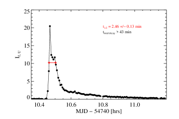
Figure 2: Example calculation of $t_{1/2}$ for a $U$-band light curve of a flare ($t_{\mathrm{peak}}=$ 10.4686 hours) on EQ Peg A on 2008 Oct 01. The time between observations ranges from $24-31$ sec. The $t_{1/2}$ is the FWHM of the light curve, illustrated in red ($t_{1/2}=2.46$ minutes). The observations ended before the flare finished, so a total decay time could not be determined.

In Figure 2, we show a light curve from 2008 Oct 01 of a large flare on EQ Peg A. We use this figure to illustrate several of the following empirical values that can be directly measured from the photometry.

• $t_{1/2}$

  To describe the time-evolution of a light curve, we define $t_{1/2}$, the full width of the light curve at half-maximum. This measures the “timescale” of the impulsive phase of the flare, including both fast rise and fast decay times. The measure of $t_{1/2}$ does not assume a functional form for the decay, which can be complex, as seen in Figure 2. We also measure $t_{1/2}$ for the light curves of spectral components (Section 3.2). In some cases, the rise time is fast compared to the photometric or spectral cadence; in these cases we must interpolate between data points to obtain $t_{1/2}$. For the example flare in Figure 2, we illustrate the $t_{1/2}$ value.

• $I_{f}$, $I_{f}+1$

  The measure $I_{f}$ is the familiar quantity in flare studies (Gershberg, 1972). It is the ratio of flare-only count flux (photons cm^-2 s^-1) in a given band, to the quiescent count flux in that band. $I_{f}+1$ is the flux enhancement, or the total count flux relative to quiescence. In solar physics, $I_{f}$ is used to express the intensity contrast. If $C(t)$ is the total count flux ratio ($\mathrm{counts}_{\mathrm{target}}/\mathrm{counts}_{\mathrm{comp}}$) in the differential photometry, normalized to 1 during quiescence, then

  $$I_{f}(t)=C(t)-1;I_{f}(t)+1=C(t)$$ (1)

  For the example flare in Figure 2, $I_{f,U,\mathrm{peak}}=20.4$.

• ED

  The equivalent duration (ED) in a given bandpass is the integral of $I_{f}$ over the duration of a flare (Gershberg, 1972). The units are seconds and multiplying by the quiescent luminosity in the band gives the energy of the flare.

• $\mathcal{I}$

  To characterize the shape of the light curve, we use an “impulsiveness index”, $\mathcal{I}$, which is defined as

  $$\mathcal{I}=I_{f,peak}/t_{1/2}$$ (2)

  The quantity $\mathcal{I}$ is a measure of the peak relative flux of a flare weighted by how fast it rises to peak and decays. Both a more luminous-at-peak flare and a smaller $t_{1/2}$ (faster timescale) can give rise to larger values of $\mathcal{I}$. We find that this measure provides a way to quantitatively sort the flares by their light curve evolution, while only using observables measured directly from the light curve.

• $\mathcal{L}$

  The specific luminosity ($\mathcal{L}$, units of ergs s^-1 Å^-1) is useful for characterizing the luminosity without the ambiguity of using a spectral window of width, $\Delta\lambda$. For example, $U$-band luminosities (and energies) assume $\Delta\lambda=700$Å whereas $B$-band luminosities (and energies) assume $\Delta\lambda=900$Å, making luminosities in the two bands not directly comparable. In some cases, we present the integrated (over wavelength) quantities L, E in typical bandpasses for comparison to previous studies. However, when comparing spectral continuum measurements, we use $\mathcal{L}$. All measures (L, E, $\mathcal{L}$) assume an isotropically-emitting source and employ the distances in Table 1.

3.2 Observational Parameters: Spectra

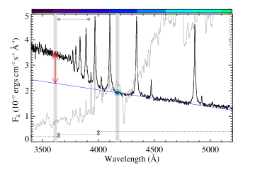
Figure 3: The flare-only emission from the peak of a flare on AD Leo from 2010 April 03 ($t_{\mathrm{peak}}=3.9120$ hours) showing the important terms from Section 3.2 used in this work. The coverage of the near-UV, intermediate, and blue-optical zones are indicated at the bottom with diamonds; the coverage of the PseudoC is indicated at the top with diamonds. The quiescent spectrum is shown in grey, and the best-fit line using the continuum windows in Table 4 is shown in dark blue. Vertical grey bars indicate the blue and red wavelength regions used to calculate C3615 and C4170; squares denote the flare-only flux values in these regions. The $\chi_{\mathrm{flare}}$ (Balmer jump ratio) is the flux of the red square divided by the flux of the blue square ($\chi_{\mathrm{flare}}$$=1.8$ in this spectrum). The red arrows indicate the excess emission, BaC3615, above the extrapolation of the linear fit to the blue-optical zone. Although $U$-band photometry was not available during this flare, $I_{f,SDSSg}+1\sim 1.28$ and $I_{f,\mathrm{C3615}}+1\sim 5.4$. For reference the visible colors for this wavelength range are indicated with the colorbar.

We now refer to Figure 3 to describe the measured parameters from the spectra. This spectrum illustrates the flare-only emission at the peak of a simple, moderate-amplitude flare on AD Leo from 2010 April 03.

• Spectral Zones:

  We divide the spectrum into four zones: the near-UV (NUV) zone ($\lambda=3420-3646$Å), the intermediate zone ($\lambda=3646-4000$Å), the blue-optical zone ($\lambda=4000-5200$Å), and the red-optical zone ($\lambda=5800-7550$Å). These are useful for our analysis of continuum variations during flares.

• C$3615$ and C$4170$

  In each spectrum, we measured the average flux in several $\sim$30Å - wide continuum windows across the DIS spectral range. The continuum windows were chosen to correspond to spectral windows free of major (and most minor) emission lines that appear during flares. The two continuum measures that we use to characterize the blue are the average flare-only flux in the wavelength region from $3600-3630$Å (denoted C3615) and the average flux in the wavelength region from $4155-4185$Å (denoted C4170). The C3615 region was chosen to be blue of the Balmer jump at 3646Å, while also red enough to obtain a reasonable signal-to-noise in small to moderate-size flares. This measure covers the approximate central wavelength of the $U$-band, which is much broader. The C$4170$ region was chosen to emulate the NBF4170 continuum filter, which is a custom continuum filter that is also employed on the solar camera ROSA (Jess et al., 2010) and stellar camera ULTRACAM (Dhillon et al., 2007). C4170 provides a measure of the continuum flux redward of the Balmer jump and unaffected by blending of high order Balmer lines. The continuum windows are summarized in Table 3 (including two other continuum windows, C4500 and C6010, used in Section 8).

• $\chi_{\mathrm{flare}}$

  To describe the flare color across the blue and near-UV wavelengths in (mostly) line-free continuum bands, we use the quantity:

  $$\chi_{\mathrm{flare}}=\mathrm{C3615}/\mathrm{C4170}$$ (3)

  The error in this quantity is obtained by propagating the standard deviation of the fluxes in C3615 and C4170,

  $$\sigma_{\chi,\mathrm{flare}}=\chi_{\mathrm{flare}}\sqrt{(\frac{\sigma_{\mathrm{C3615}}}{\mathrm{C3615}})^{2}+(\frac{\sigma_{\mathrm{C4170}}}{\mathrm{C4170}})^{2}}$$ (4)

  Formally, the uncertainties of C3615 and C4170 are the standard errors of the mean values, but some weak emission line features (e.g., Fe i, Fe ii) appear in this spectral region; therefore, a better estimate of the uncertainty in the continuum level in each window is given by the standard deviation of the flux.

  $\chi_{\mathrm{flare}}$ is similar to the Balmer jump, J, that has been measured from T Tauri star spectra (Valenti et al., 1993; Herczeg & Hillenbrand, 2008) and also in previous M dwarf flare studies in the blue to derive electron temperatures assuming an isothermal, isodensity slab of Hydrogen (Kunkel, 1970).

• BaC3615

  The quantity C$3615$ (see #2 above) is the average flare-only continuum flux from $\lambda=3600-3630$ Å  consisting of Balmer continuum emission from Hydrogen recombination and other possible components that contribute toward the continuous emission throughout these wavelengths (such as Paschen continuum and blackbody continuum). Our estimate for only the flare Balmer continuum emission at 3615Å, BaC3615, is obtained by extrapolating and subtracting a continuum that is fit to the blue-optical zone. In particular, we fit a straight line to the wavelength windows listed in Table 4 from $\lambda=4000-4800$Å (BW1 – BW6), extrapolate to $\lambda=3600$Å, and subtract an average of these extrapolated values at $\lambda=3600-3630$Å from the flare-only flux average (C3615) to obtain BaC3615. In Section 6, we find that a $T_{\mathrm{BB}}$$\sim$$10\,000$ K blackbody fits the shape from $\lambda=4000-4800$Å well and that a $10\,000$ K blackbody is approximately linear in this wavelength range. This procedure is shown for an example flare spectrum in Figure 3. Note that by definition, BaC3615 $\leq$ C3615.

• BaC

  The estimate for the wavelength-integrated Balmer continuum energy from $\lambda=3420-3646$Å. The BaC is estimated using the same fitting, extrapolation, and subtraction procedure as for BaC3615. Instead of averaging the extrapolated line value, the line extrapolation was subtracted at every wavelength in this region.

• PseudoC

  The intermediate zone (between blue-optical and NUV zones) contains the higher order Balmer lines (H7 and greater) in addition to the Ca ii H and K lines ($\lambda\sim 3934,3968$Å, respectively). Although Ca ii H is blended with H$\epsilon$ (H7) in these low resolution data, Ca ii K is resolved. Within this zone, we integrate the flare flux from $\lambda=3646-3914$Å (from the Balmer jump through H8) and refer to it as the “PseudoC” because many of the Hydrogen lines blend together (are partially or completely unresolved) at these wavelengths to form a pseudo-continuum. Again, as with the BaC, we use an extrapolation of the line-fit to the blue-optical to estimate the underlying continuum.

• S#

  We refer to the time-sequential spectrum number (starting at 0 at the beginning of each night) with an S#. These numbers refer to the $n$B subcategory of spectra used for blue continuum analysis as described in Section 2.2 (see also Table  2).

• Times

  The times on the light curves indicate the number of hours elapsed on the respective MJD from Table 2. Times always refer to midtimes of the exposure. The times for the flare data from 2009 Jan 16 are given in “elapsed hours from flare start”, as used in Kowalski et al. (2010); to obtain the number of hours elapsed on MJD 54847, add 4.2483 hours to the number of elapsed hours from flare start.

3.3 General Descriptive Terms

Additional terminology used to describe the photometry and spectra are the following:

• Impulsive Phase

  An impulsive phase consists of a fast rise, peak, and fast decay of the light curve.

• “Peak” or “maximum continuum emission”

  “Peak” or “maximum continuum emission” always refer to the maximum value of C3615 during a flare. The peak times are given for each flare in Table 5.

• Gradual Decay Phase

  Gradual phase emission is observed during times of slowly rising or slowly decreasing emission. Following HP91, the “gradual decay phase” is defined as the turnover from fast to slow decay. The gradual decay phase spectra are chosen from the section of the light curve as near to the break from fast decay to slow decay as possible. We select three spectra around a time when C3615 is not changing rapidly so that the spectra can be coadded to increase the signal-to-noise without largely affecting the interpretation of atmospheric parameters. The red vertical dashed lines in Figures 43 – 61 in Appendix B indicate the times that we selected to represent the gradual decay phases for the flares in our sample. The gradual decay phase times analyzed for each flare are given in Table 5.

• “blackbody continuum component”

  This term refers to a continuum slope that matches the slope of a Planck function with temperature $T_{\mathrm{BB}}$. A “hot blackbody” is used to designate a blackbody continuum component with $T_{\mathrm{BB}}$$\gtrsim 8500$ K.

4 The Flare Atlas

The Flare Atlas refers to the collection of time-resolved spectra and photometry of the twenty flares analyzed in this paper. In this section, we present overview figures and tables, and we briefly describe the categories of flares based on light curve morphology. For detailed descriptions of each of the flares, we refer the reader to Section 3.4 of Kowalski (2012). The spectra (original flux and flare-only flux) and photometry ($I_{f}+1$) for all nights are available through the VizieR service.

4.1 Broadband Light Curves

The impulsiveness index ($\mathcal{I}$) provides the main light curve morphological classification scheme employed in the remainder of the paper. For our flare sample, $\mathcal{I}$ ranges from $0.02-100$. The impulsive flares (IF) are those that have $\mathcal{I}>1$, whereas the gradual flares (GF) have $\mathcal{I}<1$. For flares that are close to this dividing line ($\sim 0.6-1.8$), we assign the classification hybrid flares (HF), as these flares have a prominent impulsive phase (or several impulsive phases) but also share properties with the gradual flares. We also considered the fast and slow flare classification scheme from Dal & Evren (2010), but this grouping employs a total decay time measurement; in some cases, poor weather, a standard star sequence, or secondary flares interrupted the decay measurements. Using $t_{\mathrm{1/2}}$ (in the definition of implusiveness) bypasses the ambiguities with measuring precise start and stop times.

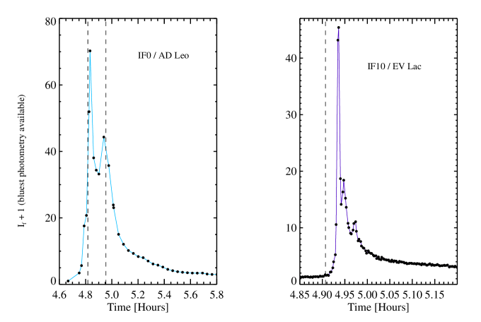
Figure 5: Same as in Figure 4, for the two impulsive flares with lower time-resolution and limited wavelength coverage in the near-UV and blue-optical. The vertical dashed black lines indicate the time of maximum C3615. For IF0, we have indicated the two times of maximum C3615 from the spectra. The integration times for IF10 were long and the midtime of the spectrum with maximum C3615 is before the rise phase; please refer to Figure 53 in Appendix B.

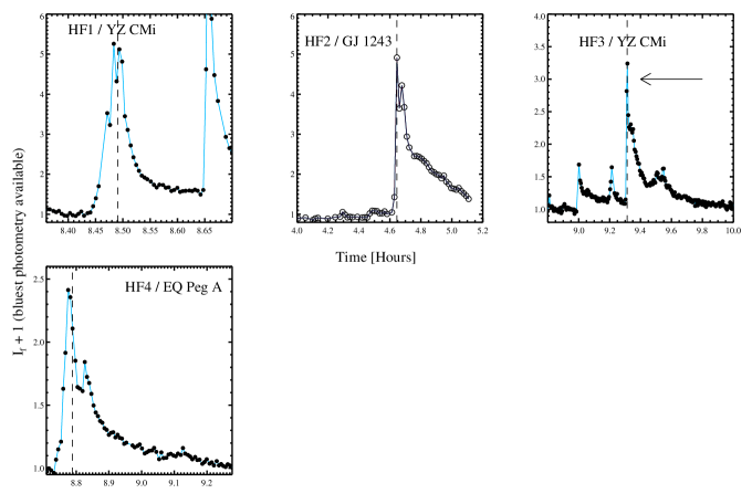
Figure 6: Same as in Figure 4, for the hybrid flares. The vertical dashed black lines indicate the time of maximum C3615. Open circles show spectrophotometry estimations of the Johnson $U$ band. An arrow indicates the HF3 event.

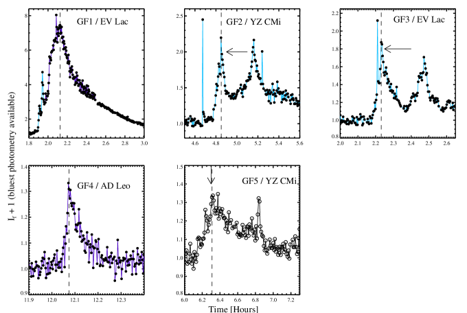
Figure 7: Same as in Figure 4, for the gradual flares. The vertical dashed black lines indicate the time of maximum C3615. Open circles show spectrophotometry estimations of the Johnson $U$ band. Arrows indicate the GF2, GF3, and GF5 events.

The bluest available photometry (SDSS $u$, Johnson $U$, or SDSS $g$) for the flares in our sample are shown in Figure 4 (nine impulsive IF events), Figure 5 (two impulsive IF events – IF0 and IF10 – with less data), Figure 6 (four hybrid HF events), and Figure 7 (five gradual GF events). In Appendix B, we show figures of each flare with the integration times of the spectra (Figures 43 – 61) and the spectrum numbers (S#’s) indicated. IF0 on AD Leo from HP91 is known as the “the Great Flare”, and IF1 on YZ CMi (Kowalski et al., 2010) is known as “the Megaflare”. In the decay phase of IF1, we refer to the sub-peak at $t=2.1441$ hours as the “Megaflare decay secondary peak #2” or “MDSF2”.

From the light curves, it is apparent that our sample contains a diverse set of peak amplitudes, total durations, and light curve morphologies. The naming convention (IF, HF, and GF) and the ordering of the flares within this classification scheme is based on the value of $\mathcal{I}$ as detailed in Section 3.1. Table 6 summarizes the key properties of the $U$-band photometry: flare ID (col 1), star name (col 2), date (col 3), time of peak C3615 (col 4), $I_{f,U}+1$ at peak photometry (col 5), equivalent duration in $U$ (col 6), $U$-band energy (col 7), $U$-band luminosity at peak photometry (col 8), $t_{1/2,U}$ (col 9), and $\mathcal{I}$ (col 10). The time-integrated photometric quantities are calculated only during the time period when spectra were obtained. Note that the time of peak photometry and time of peak C3615 may not precisely coincide due to the different cadences and integration times.

4.2 Spectra

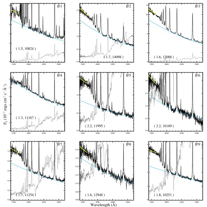
Figure 8: The spectra at maximum continuum emission (C3615). The black is the flare-only emission, the dotted line is the quiescent spectrum. The best-fit Planck function to the blue-optical region is shown in light blue. The yellow curve at $\lambda<3646$Å is the best-fit Planck function scaled to the C$3615$ flux. In parentheses, the $\chi_{\mathrm{flare,peak}}$ and the best-fit color temperature are given. The S#’s and times of these spectra are given in Table 5. See Section 6 for more details about the continuum properties at these times.

In Appendix C, we present the Flare Atlas with a time-sequence of flare-only spectra from $\lambda=3400-7500$Å for each flare event. In Figures 8  –  11, the flare-only spectra at maximum continuum emission (i.e., maximum C3615) are presented in the same order as the photometry in Figures 4 – 7. The quiescent levels are shown as dotted lines for comparison. Table 7 gives the $I_{f,\mathrm{C4170,peak}}$, $t_{1/2,\mathrm{C4170}}$, $\chi_{\mathrm{flare,peak}}$, and $\chi_{\mathrm{flare,decay}}$ for each flare as a reference; these values are important constraints for flare models (Section 9). A detailed analysis of the continuum will be discussed in Section 6; here, a simple Planck function (light blue line) has been fit to the windows in the blue optical zone ($\lambda=4000-4800$Å; BW1 – BW6 in Table 4) to parameterize the slope of the continuum. The best-fit temperatures and $\chi_{\mathrm{flare,peak}}$ values are shown in parentheses. Except for GF1 (and possibly GF3 and GF5), the GF events are generally too faint for an accurate continuum fit in the blue-optical zone.

There are varying amounts of the excess continuum at $\lambda\lesssim 3640$Å above the extrapolation of the blackbody (blue line), especially among the IF events. The HF and GF events have large amounts of excess continuum at $\lambda\lesssim 3640$Å. The spectral trends in the near-UV zone for the IF, HF, and GF events are similar to the underlying blackbody curves. To illustrate this, we scale the light blue blackbody curves to the flux at $\lambda=3600-3630$Å and show these in yellow, which basically have the same slopes as the light blue fits.

4.3 Overview of the Flare Atlas

The flares in our sample represent relatively large amplitude and high energy events on dMe stars. For example, the average $U$-band flare energy on YZ CMi is $\sim 0.03\times 10^{32}$ ergs (Lacy et al., 1976), which is slightly smaller than the lowest energy flare (IF8) on this star in Table 6. The IF events have a large spread of amplitudes from low ($I_{f,peak}+1\sim 2.5-3$) to very large ($I_{f,peak}+1>10$). The IF events also generally have a classical, simple shape: a fast-rise, a fast decay, and a more gradual decay beginning at a low level, $\sim 20$% or less, relative to the peak. Durations range from several minutes (e.g., IF6, IF8) to several hours (e.g., IF1, IF3). Some IF events have secondary flares but they are usually dominated by a single, large-amplitude peak. The HF events also have fast rise components, but they exhibit marked deviations from the classic flare shape, such as multiple continuum peaks of comparable amplitude during the impulsive phase (e.g., HF1) and an elevated or prolonged decay phase (e.g., HF2). These flares are low to moderate amplitude ($2<I_{f,peak}+1<5$) and usually longer lasting ($>1$ hour) than the IF events of comparable amplitude. The GF events are low-amplitude ($I_{f,peak}+1<2.2$) except for GF1 which has $I_{f,peak}+1\sim 8$. The rise phases are notably slower, although they can have distinct periods of faster and slower emission; and may be accompanied by intermittent peaks (e.g., GF1 and GF3). However, these continuum peaks do not significantly contribute to the overall timescales, which can be several hours for even the low amplitude flares.

There is often another local maximum (i.e., a secondary flare) just after the first peak but before the gradual decay phase. Secondary flares are especially evident in IF0, IF1, IF3, IF10, HF2, and HF4. Secondary flares usually occur at about half the peak flux level or less. Although the four largest amplitude events all have secondary flares (with $\sim$15 or more occurring during IF1), lower amplitude events also show them. IF4 is a large-amplitude event that shows a stall in the fast decay resulting in a nearly constant flux level before continuing a fast decay. This also may be interpreted as a relatively low-amplitude secondary flare.

In addition to the quantitative “impulsive”, “hybrid”, and “gradual” classification schemes, we find the following descriptive groupings using the data in Tables 6, 7 in addition to the light curve data (not shown here; see Chapter 3 of Kowalski, 2012) of the spectral components from Section 3.2.

• Simple, classical flares (IF2, IF5, IF7, IF9): These flares have moderately large amplitudes ($I_{f,U,\mathrm{peak}}+1\sim 5-12$) and energies ($E_{U}\sim 2\times 10^{31}-2\times 10^{32}$ ergs). A defining characteristic is that the $U$-band (or bluest photometry) follows the evolution of C4170, which in fact, holds for most of the flares. The different timescales of decay between the spectral components are evident: although C4170, BaC3615, and H$\gamma$ vary from fastest to slowest, there is a spread of relative $t_{1/2}$ values, with IF9 having the smallest ratio of $t_{1/2,\mathrm{C4170}}/t_{1/2,\mathrm{BaC3615}}$. Except for IF7, these flares don’t have obvious secondary flares in the decay.

• Low amplitude flares (IF6, IF8, GF2, GF3): The low amplitude flares have $I_{f,U,\mathrm{peak}}+1\sim$2 (GF) and $\sim$3 (IF). There are both complex and simple events in this group, and the durations range from minutes to hours. These flares have lower energies: the low-amplitude short-duration flares have $E_{U}\sim 5\times 10^{30}$ ergs and the low-amplitude long-duration flares have $E_{U}\sim 10^{31}$ ergs in their first main peaks; the complex flares are more than 10 times as energetic as the simple flares, even though the simple flares have larger peak amplitude in $U$ (or $u$).

• Multiple-peaked, medium amplitude flares (HF1, HF2, HF3, HF4): These are medium amplitude flares with multiple peaks in the impulsive phase, having $I_{f,U\mathrm{peak}}+1\sim 2.5-5.5$. These flares are all hybrid flares (HF type). Generally, in the HF flares, the evolution of the $U$-band closely matches the evolution of the BaC3615, whereas typically in the IF flares, the evolution in the $U$-band matches the evolution in C4170. In these flares, $\chi_{\mathrm{flare,peak}}$ is 2.3 – 3.

• High energy flares (IF0, IF1, IF3, IF4, IF9, IF10, GF1): The high energy flares have $E_{U}>3\times 10^{32}$ ergs. The most impulsive flares (except IF2) tend to be the most energetic. C4170 and $U(ug)$ photometry track each other well in the high energy flares, whereas the BaC3615 is more similar in evolution to the H$\gamma$ line. Secondary flaring to varying degrees is observed in all cases.

• Low amplitude, simple gradual flares (MDSF2, GF4, GF5): These flares have a moderate amount of energy ($E_{U}\sim 10^{31}-10^{32}$ ergs) for their low peak-amplitudes. Interestingly, they lack a prominent fast decay phase after the peak emission. In GF5, short impulsive events are observed later in the flare decay. MDSF2 during the IF1 gradual decay phase is included in this group; its values of $E_{U}\sim 10^{32}$ ergs and $\mathcal{I_{U}}\sim 0.6$ qualify it a high energy, hybrid/gradual flare.

4.3.1 General Relationships Between Spectral and Photometric Properties

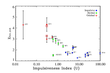
Figure 12: The peak properties of the flare sample: $\chi_{\mathrm{flare,peak}}$ (or Balmer jump ratio) shows a global trend with the impulsiveness index, $\mathcal{I}$ of the flare. The flares are colored according to their IF/HF/GF designation. We show a point for $\mathcal{I}\sim 0.6$ for MDSF2 and $\mathcal{I}\sim 27$ for the entire IF1 event given the same $\chi_{\mathrm{flare,peak}}$$\sim 1.5$. Note that the $\chi_{\mathrm{flare,peak}}$ and $\mathcal{I}$ for IF10 were obtained at a largely different cadence. For GF3 and GF2, we show $\chi_{\mathrm{flare,peak}}$ for the secondary peaks in the events ($\chi_{\mathrm{flare,peak}}$$=$3.3 and 4.2, respectively) as red square symbols. The $\chi_{\mathrm{flare,peak}}$ for GF4 is exluded from Figures 12, 13, and 14 because of its large uncertainty (see text).

The general relationships between spectral properties ($\chi_{\mathrm{flare,peak}}$, H$\gamma$/C4170) and photometric $Uug$ light curve properties ($\mathcal{I}$) of the Flare Atlas are summarized with three figures, Figures 12  – 14. Figure 12 ($\chi_{\mathrm{flare,peak}}$ vs. the impulsive index, $\mathcal{I}$) indicates that the instantaneous continuum shape at maximum amplitude in the broadband light curve is linked to the overall evolution of the flare. From this figure (see also values in Table 7), it is evident that the most impulsive flares have the lowest $\chi_{\mathrm{flare,peak}}$, with most $\lesssim 1.8$ and all $\lesssim 2.2$. The HF events have intermediate values, $\chi_{\mathrm{flare,peak}}$$\sim 2.3-3$, and the GF events have larger but more uncertain values (besides GF1), $\chi_{\mathrm{flare,peak}}$$\sim 3+$. The errors on $\chi_{\mathrm{flare,peak}}$ are typically 0.01 – 0.12 (corresponding to relative errors of 3 – 10%), but some flares have significantly larger errors with the GF events generally having the largest uncertainties. We do not consider the $\chi_{\mathrm{flare}}$ values with $\sigma_{\chi_{\mathrm{flare}}}/$$\chi_{\mathrm{flare}}$$>0.2$. This excludes GF4 from $\chi_{\mathrm{flare,peak}}$ analysis and IF5, IF6, IF8, HF4, GF2, GF3, GF4, and GF5 from $\chi_{\mathrm{flare,decay}}$ analysis. Using standard error propagation, we determine the confidence levels by which the IF, HF, and GF sequence is ordered according to the $\chi_{\mathrm{flare,peak}}$ parameter. We find that IF9 and HF1 are separated by 4.5$\sigma$, HF4 and GF1 are separated by $<$1$\sigma$, HF1 and GF1 are separated by $5\sigma$, and IF5 and IF9 separated by almost $4\sigma$. The differences in $\chi_{\mathrm{flare,peak}}$ are generally more significant between the IF and HF events than for the HF and GF events; this is not surprising given that the IF events tend to have the larger signal-to-noise due to their larger amplitudes. We conclude that the differences in $\chi_{\mathrm{flare,peak}}$ are significant between IF, HF, and GF events, and even between certain IF events.

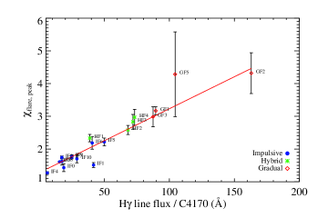
Figure 13: The $\chi_{\mathrm{flare,peak}}$ vs the ratio of H$\gamma$ to C4170 (at peak C4170). There is nearly a linear relationship, which is shown as a red line (see text). The point for IF1 corresponds to the peak C4170 of MDSF2.

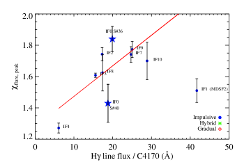
Figure 14: The $\chi_{\mathrm{flare,peak}}$ vs the ratio of H$\gamma$ to C4170 (at peak C4170) for the low values of $\chi_{\mathrm{flare,peak}}$ and H$\gamma$ to C4170 ratio in Figure 13. The linear relationship fit to the entire sample is shown as a red line (see text). The point for IF1 corresponds to the peak C4170 during MDSF2. This figure shows the two main peaks (S#36 and S#40) of IF0 as star symbols.

In Figures 13 – 14, we show the H$\gamma$ line flux divided by the continuum C4170 flux (both taken at peak C4170; essentially this is the equivalent width of the C4170 flare continuum in units of Å). The flares are color-coded by the IF/HF/GF designation. Figure 14 shows a narrower range of values than Figure 13 where IF2, IF3, IF7 , IF8, IF9, and IF10 cluster together at $\chi_{\mathrm{flare,peak}}$ $\sim 1.6-1.8$. The first and second peaks of the Great Flare (IF0) are also included in Figure 14. Note that IF8 and IF3 are the smallest and largest amplitude impulsive flares (with full spectral and time coverage) respectively on YZ CMi, yet they show very similar peak characteristics. IF4 has the lowest $\chi_{\mathrm{flare,peak}}$ ($\sim$1.3) and also line-to-continuum ratio ($\sim$6)

In Figures 13 – 14, we see that the light curve morphology and $\chi_{\mathrm{flare,peak}}$ are related to the ratio of H$\gamma$/C4170. The IF events have H$\gamma$/C4170 $\lesssim$50 (most IF events fall below 30), the HF events show 38$\lesssim$H$\gamma$/C4170$\lesssim$75, and the GF events show 85$\lesssim$H$\gamma$/C4170$\lesssim$165. We find a very strong relationship between $\chi_{\mathrm{flare,peak}}$ (recall, $\chi_{\mathrm{flare,peak}}$ $=$ C3615/C4170) and H$\gamma$/C4170:

$$\chi_{\mathrm{flare,peak}}\approx 0.020(\pm 0.002)H\gamma/\mathrm{C4170}+1.28(\pm 0.05)$$ (5)

Among the IF events, IF3, IF5, IF7, IF8, and IF9 fall closest to the best fit line. Although IF5 and IF6 are the impulsive flares (see Figure 4) with the largest values of $\chi_{\mathrm{flare,peak}}\sim 2.2$, they also have relatively large values of H$\gamma$/C4170 $\sim$40 – 50. IF1 is an outlier (with much more relative H$\gamma$ radiation for the $\chi_{\mathrm{flare,peak}}$ value predicted by the red line), as the peak data correspond to the peak of a secondary flare (MDSF2) during the gradual decay phase. As $\chi_{\mathrm{flare}}$ is effectively a measure of the Balmer jump height, this relation implies that flares with larger Balmer jumps relative to the C4170 flux have larger Balmer line fluxes relative to C4170 flux. This implies a connection between the relative amount of Balmer line radiation and Balmer continuum radiation. $\chi_{\mathrm{flare}}$ is thus a very important quantity because it can be measured without spectra (Kowalski et al., 2011b), yet apparently it can be used as a diagnostic of the Balmer line and continuum radiation.

5 Emission Line Analysis

Emission lines are used to probe the temperatures and densities, and therefore different heights, of a flaring atmosphere by matching models to the observations. As current radiative-hydrodynamic (RHD) models predict line flux decrements and profiles that are relatively in agreement with the observations (Allred et al., 2006), heights of formation (via the contribution function, e.g. Magain, 1986; Carlsson & Stein, 1997; Carlsson, 1998) can be used to constrain the time-evolution of heating at different layers in the atmosphere (Hawley & Fisher, 1992, e.g.,). Ultimately, whatever heating mechanism is used to explain the continuum properties during flares must also be consistent with the observed emission line properties. For example, Cram & Woods (1982) found that the model atmosphere that best matched the continuum observations did not match the corresponding properties of H$\alpha$. As a result, they suggested a combination of several models to explain the observations.

An extensive analysis of the Balmer line broadening, line flux and energy decrements, and H$\alpha$ time evolution for the Flare Atlas can be found in Kowalski (2012). Here, we present the emission line results that 1) are most relevant to understanding the origin of the continuum and 2) would most greatly benefit from future observations (e.g., at higher cadence).

5.1 The H$\gamma$ line and its relation to the continuum

As was discussed in Section 4.3.1 (Figures 13 – 14), a larger ratio of H$\gamma$ flux to C4170 generally results from flares with larger $\chi_{\mathrm{flare,peak}}$. Therefore, the height of the Balmer jump is related to the relative amount of Balmer line radiation produced at peak emission. H$\gamma$ is a useful diagnostic because it is a strong, easily measured line, in both high and low flaring states. This line is also the highest order Hydrogen line calculated in most RHD models to date. Furthermore, its properties have been studied extensively in the past for dMe flares. The $U$-band is widely used for flare monitoring (Moffett, 1974), and it is a diagnostic of the continuum flux and energy, since colorimetry studies have shown the peak of the white-light occurs in the $U$-band or at shorter wavelengths (Hawley & Fisher, 1992).

The $U$-band contains higher order Balmer lines and Ca ii H and K, but $\gtrsim$90% of the $U$-band energy is due to continuum radiation (Doyle et al., 1988, see also HP91). It is a well-established property that the Balmer lines evolve more slowly than the continuum, staying elevated longer (Kahler et al., 1982) and sometimes peaking as late as the end of the impulsive phase (HP91, García–Alvarez et al., 2002; Gurzadian, 1984). The time-integrated energies scale over approximately 4.5 orders of magnitude with $E_{U}\sim 25\times E_{H\gamma}$ (HP91). Using a larger sample in this study, we find that the BaC3615 component of the $U$-band is even better correlated with the properties  –  including peak luminosity, total energy, and time-evolution.

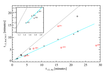
Figure 15: The $t_{1/2}$ values of BaC3615 versus the values for the H$\gamma$ line. The inset has the same axes, showing the flares with the smallest values of $t_{1/2}$. The red squares with labels represent impulsive or hybrid flares with 2 – 3 peaks; the crosses are impulsive or hybrid flares with single peaks, and the open circles are gradual flares. The dotted line is the 1:1 line and the solid light blue line is the linear fit to the IF and HF events with single peaks (see text). Note that only an upper limit of $t_{1/2,\mathrm{BaC3615}}<$400 sec was determined for IF0.

Here, we analyze the timing in detail. Figure 15 shows the relation between $t_{1/2,H\gamma}$ and $t_{1/2,\mathrm{BaC3615}}$. We find a linear relation among the IF and HF events without multiple peaks (crosses). The fit to these flares is shown as a light blue line, given by

$$t_{1/2,\mathrm{BaC3615}}\approx 0.54(\pm 0.01)t_{1/2,H\gamma}+0.4(\pm 0.1)$$ (6)

In other words, $t_{1/2}$ is twice as fast in the Balmer continuum as in H$\gamma$.

The GF events (shown in open circles) follow a different trend with nearly equal timescales in H$\gamma$ and BaC3615. GF1 is a multiple-peaked flare, and it produces copious BaC3615 with a long timescale. The IF and HF events with 2 – 3 peaks (IF0, IF4, HF1, HF2, and HF4) spaced relatively close in time are shown with red squares and are labeled. IF4 and HF2 are double-peaked flares and are apparently outliers (the red squares with $t_{1/2,H\gamma}\sim 16$ minutes). IF4 falls closer to the GF distribution, and HF2 (also possibly IF0) have much faster BaC3615 timescales given the H$\gamma$ timescale predicted by the light blue line. HF1 and HF4 fall near the single-peak distribution and the GF distribution, respectively. Note that $t_{1/2}$ depends on which peak dominates and also how it is measured (e.g., the time delay between multiple peaks). A larger sample of double-peaked IF and HF events would constrain their different timing behavior in H$\gamma$ and BaC3615.

The IF0, IF4, and HF2 events exhibit large delays of $\sim$$10,4$, and 3 minutes, respectively, between the times of maximum continuum (C3615) and maximum line (H$\gamma$) emission, suggesting a difference in the heating and cooling timescales of the continuum and line radiation during the impulsive phase. We find that these relatively common, large lags result when secondary continuum peaks lag the primary events, as discussed above for Figure 15. For most flares without a relatively large secondary event following closely after the first peak, however, there is a difference of less than one minute (and in most flares, no lag within the time resolution of the spectra) between the peak times of the continuum and H$\gamma$ line. The short delay in peak times of $<1$ minute suggests that a common heating mechanism produces the impulsive phase of line and continuum radiation during high energy flare events with relatively simple morphology, such as IF3 and IF9. The largest (apparent) lags of 18 and 15 minutes result in the GF2 and GF3 events, which have two (or more) primary peaks in C3615 of similar amplitude separated by large amounts of time ($\gtrsim 15$ minutes). However, considering the time only around the first impulsive phase in the GF2 and GF3 events, the lags between the local maxima of H$\gamma$ and C3615 are 0 – 0.5 minutes. We speculate that lags are the result of superimposed flare events, and the emission components with different decay timescales (e.g., H$\gamma$ and C3615) add to produce different timings of the peaks. We plan to investigate this further in a future paper.

5.2 The Hydrogen Balmer “time-decrement”

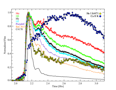
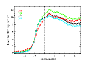
Figure 16: (Left) Line and continuum evolution for IF3. C4170, BaC3615, PseudoC, H$\alpha$, H$\beta$, H$\gamma$, H$\delta$, Ca II K, and He I$\lambda$4471 light curves are plotted normalized to their peak fluxes. The vertical dotted line corresponds to the time of peak continuum (S#31). (Right) Expanded view of the rise phase, peak, and initial decay of IF3 for the H$\alpha$, H$\beta$, H$\gamma$, and H$\delta$ line fluxes. Note the “S”-shape in the rise phase morphology of H$\beta$, H$\gamma$ and H$\delta$. All four lines reach maximum in the same spectrum. Note, that the H$\beta$, H$\gamma$ and H$\delta$ lines diverge from a common flare flux at S#29, just before the peak.

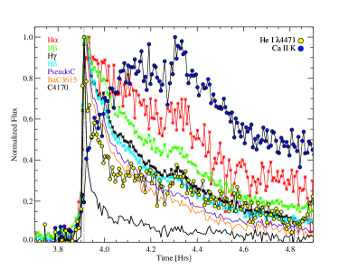
Figure 17: Line and continuum evolution for IF9. Symbols same as in Figure 16.

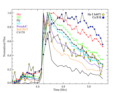
Figure 18: Line and continuum evolution for HF2. Symbols same as in Figure 16.

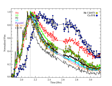
Figure 19: Line and continuum evolution for GF1. Symbols same as in Figure 16.

We connect the timing properties of the Hydrogen Balmer components with a simple new relation, the time-decrement. We use the exceptionally high-quality data covering the time-evolution of the Hydrogen lines in flares IF3, IF9, HF2, and GF1 (Figures 16, 17, 18, and 19, respectively) to show this relationship and how it varies among flare type. In addition to H$\alpha$, H$\beta$, H$\gamma$, and H$\delta$, we show the continuum evolution of PseudoC, BaC3615, C4170, Ca ii K, and He i $\lambda 4471$. The fluxes are normalized to their peaks to illustrate the different decay trends. Figure 16 (bottom panel) also shows the rise phase in detail for the absolute fluxes of H$\alpha$, H$\beta$, H$\gamma$, and H$\delta$.

From the data in Figures 16  –  19, it is evident that the higher order Balmer lines have a faster decay time compared to the lower order lines, declining to a lower relative flux by the end of the impulsive phase. This effect was noted by Doyle et al. (1988) and HP91. According to $t_{1/2}$, the ordering of the components from fastest to slowest is C4170, He i $\lambda$4471, BaC3615, PseudoC, H$\delta$, H$\gamma$, H$\beta$, H$\alpha$, and Ca ii K. H$\gamma$ and H$\delta$ have rather similar decay rates, but H$\gamma$ is apparently slower. Ca ii K will be discussed in Section 5.3.

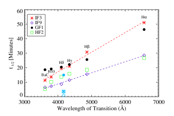
Figure 20: The $t_{1/2}$ vs. wavelength (time-decrement) of the Balmer emission features in flares IF3, IF9, and GF1 and HF2. The $t_{1/2}$ value for H10 is shown as a representative member of the PseudoC. The higher order (shorter wavelength) lines evolve faster, and the evolution timescale is inversely proportional to the energy of the transition. Linear fits to the Hydrogen Balmer features are show as a red dashed line for IF3 and as a purple dashed line for IF9. The $t_{1/2,\mathrm{C4170}}$ values are shown as light blue symbols.

To connect the timescales across the Balmer series, we plot the $t_{1/2}$ value of each transition as a function of the wavelength of the transition in Figure 20 for IF3 (red asterisks), IF9 (black diamonds), GF1 (black circles), and HF2 (black squares). An estimate of $t_{1/2}$ for the H10 line (using an extrapolation from the blue-optical as the underlying continuum) from the PseudoC component is included as well as the value of $t_{1/2}$ for BaC3615. Remarkably, this “time-decrement” relationship among the Balmer spectral components appears nearly linear in wavelength space for the two classical, impulsive (IF) events in the figure. The time-decrement for IF3 is fit with a linear relation (red dashes) to show the trend

$$t_{1/2}=0.014\lambda-36.96.$$ (7)

IF9 has a similar time-decrement as IF3 but with a factor of $\sim$1.7 shorter timescales. The linear relation for IF9 (purple dashes) is

$$t_{1/2}=0.0077\lambda-21.83$$ (8)

The scaling between the time decrement relationships of these two flares indicates a fundamental similarity between the heating/cooling processes of Balmer emission produced in medium and large classical flares. A simple discussion of the physical parameters that produce the linear time-decrement of the IF events is given in Section 11.1, but this phenomenon should be investigated with detailed radiative-hydrodynamic models.

The gradual flare GF1 has the same $t_{1/2}$ for H$\gamma$ and H$\delta$ as IF3, but the lower order line evolution is faster and the higher order line evolution is slower: in other words, the time decrement for GF1 is flatter compared to the impulsive flares.

The time-decrement of HF2 is flat for the lower order lines and steepens for the higher order lines and BaC3615. HF2 has two continuum peaks with a highly elevated gradual decay phase, and its overall time evolution is a result of the combined (i.e., spatially unresolved) heating during the two emission peaks. Recall that in Figure 15 (Section 5.1) we compared the $t_{1/2}$ of H$\gamma$ and the BaC3615 between all flares, and found a general relation for the simple events while complex events, such as HF2, behaved differently. Figure 20 elucidates this difference, consistent with its hybrid classification. The time-evolution of HF2 is studied further in Appendix D of Kowalski (2012). To understand the time-decrement of HF2, it will be necessary to superpose two simple events (each with a linear time decrement) with the spacing of the two peaks in HF2. A study that explores the results of superposing emission of simple events will be presented in a future paper.

The $t_{1/2,\mathrm{C4170}}$ values (Table 7) for these four events are also shown in Figure 20 as light blue symbols. The very fast evolution ($t_{1/2}=$1 – 15 minutes) of C4170 does not follow the time-decrement relationship among the Balmer emission components. The ratio of the $t_{1/2,\mathrm{C4170}}$ values (not used in the linear fits) between IF3 and IF9 is $\sim$3.8 which is larger than the scaling factor of $\sim 1.7$ between the time-decrements of the respective Balmer components. This indicates that several heating/cooling processes are simultaneously present during the flare – a dominant process for the Balmer emission component, which approximately scales (e.g., similar heating over larger area) between classical flares, and a dominant process for the C4170 emission component, which does not scale in the same way between classical flares. Therefore, it is possible that these different heating processes are present for different lengths of time (e.g., the C4170 heating process only in the impulsive phase). If the C4170 originates from the same (or similar) heating process that produces the Balmer lines  –  as was concluded from the similar timing of the peaks of H$\gamma$ and C3615 for these two flares (Section 5.1  –  the fast timescale of C4170 either implies formation in a denser region of the atmosphere where the cooling is more efficient or a threshold in the strength of the heating process that can produce C4170.

Additionally, the time-evolution of C4170 gives important insight into how the heating processes (and hence time-decrement) vary between the types of flares (IF, HF, GF). The $t_{1/2,\mathrm{C4170}}$ is relatively large for GF1, and this may be related to the general flatness of the Balmer time-decrement relation. In other words, the GF1 event has similar timescales for its spectral components, implying that they are more closely related in their formation and persistence over time. The $t_{1/2,\mathrm{C4170}}$ for HF2 is slightly large compared to the Balmer time-decrement, and this flare consists of two temporally resolved, yet spatially unresolved, peaks superposed. The different heating properties in the two peaks of HF2 may generate the mixed time-decrement behavior. The IF events show a simple, linear relationship among the Balmer emission components, yet they also exhibit the largest difference between Balmer emission and C4170 timescales. The timing of the C4170 and Balmer series are important constraints for consistently modeling these spectral components together.

5.3 The Ca II K Neupert-like Effect

The formation and time evolution of the Ca ii K line has long been a mystery, including why it responds slowly in flares and peaks after the Balmer lines. It has been associated with formation in the lower chromosphere in time-dependent, nonthermal electron heating models of the impulsive phase (Abbett & Hawley, 1999; Allred et al., 2006), and phenomenological modeling has shown that Ca ii K emission can also be associated with a hotter, higher region in the flaring chromosphere (Schmidt et al., 2012). Models of coronal X-ray backwarming have shown that relatively large amounts of Ca ii emission originate from a range of heights in the flare chromosphere for $T\sim 5000-7600$ K (Hawley & Fisher, 1992). The timing properties have been interpreted with a scenario in which hot flare loops cool down to the temperature of Ca ii K formation (Gurzadian, 1984; Houdebine, 2003; Crespo-Chacón et al., 2006), but this remains to be tested with radiative hydrodynamic models of the gradual decay phase.

The Neupert effect (Neupert, 1968) is an observed relation between the signatures of impulsive phase nonthermal particles and gradual phase coronal heating. The Neupert effect is usually reported as the proportionality between the integral of nonthermal microwave, hard X-ray, or white-light emission and the luminosity of thermal soft X-rays. The Neupert effect has been observed in solar (Dennis & Zarro, 1993) and stellar (Hawley et al., 1995; Guedel et al., 1996; Osten et al., 2004; Fuhrmeister et al., 2011) flares, and is a fundamental aspect of the standard flare model. It is usually interpreted in terms of the chromospheric evaporation process (Fisher et al., 1985), whereby the nonthermal particles impact chromospheric material, which then ablates into the corona and emits thermal radiation at millions of degrees well into the gradual phase of the nonthermal particle emission. The models of Hawley & Fisher (1992) showed that the Ca ii K line flux evolution during the Great Flare could be produced from X-ray backwarming from a flare corona at $T\sim 10$ MK. Here we investigate whether Ca ii K follows a Neupert effect representing the gradual phase emission (like soft X-rays) using C4170 to represent the impulsive phase emission.

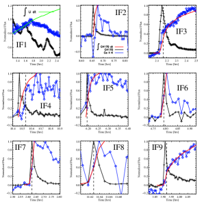
Figure 21: Ca ii K fluxes compared to the flux of C4170 and the cumulative integral of C4170 (solid red line) for the IF events with DIS data. Because IF1 did not have complete spectral coverage, we plot the Ca ii K flux against the $U$-band flux and the cumulative integtral of the $U$-band (solid green line). The peak fluxes are normalized to 1. The times of maximum H$\gamma$ line emission are indicated by vertical dashed lines. If elevated, the preflare value in Ca ii K was subtracted from the light curves. Note that the Ca ii K variations in the light curve of IF8 are not significant. The Ca ii K flux follows the cumulative integral of C4170 particularly well (for times before the maximum Ca ii K value) for most IF events, except for IF2 and IF4.

Ca ii K is the most gradual line in the intermediate and blue-optical spectral zones (Figures 16, 17, 18, and 19); well-known characteristics are a longer rise time than the Balmer lines, a late peak in the beginning of the gradual decay phase, and a slow return to quiescence (e.g., HP91). In Figures  21  –  22, we show the flux of Ca ii K (blue diamonds), the flux of C4170 (crosses) and the cumulative integral of C4170 (red lines) for flares with ARC 3.5-m/DIS data. We calculate the cumulative integral of C4170 until the time of Ca ii K maximum, which in some cases occurs between the end of the impulsive phase and beginning of the gradual decay phase (IF0, HF1, HF2, GF1) and in some cases occurs deep into the gradual decay phase (IF3, IF9). This variation in the timing of the Ca ii K peak has been seen in the literature (Houdebine, 2003). There is a varying degree of similarity in the evolution between the Ca ii K line and the cumulative integral of the continuum. The closest similarities are found for the flares IF6, IF7, IF9, HF1, HF2, GF1, and GF2; the largest differences for IF2, IF3, IF4, and GF3. For the fastest flares, it would be useful to test this relation with higher cadence data. For the flare IF1, we show the cumulative integral of the $U$-band light curve scaled to match the maximum of the Ca ii K light curve. Despite not knowing if the maximum of Ca ii K within this time window (at $t\sim 1.75$ hours) is the absolute maximum for the flare, the cumulative integral of $U$ follows the Ca ii K from $t=1.3$ hours to $t=1.75$ hours. In some flares, the Ca ii K line evolution does not obviously respond during the first part of the impulsive phase, showing evidence of a delay compared to C4170; this is seen in IF3, IF4, HF1, and HF3. Ca ii K shows a decrease (although by a small amount) relative to the previous spectrum in the impulsive phase of the flares IF2, IF4, IF5, IF9, HF1, and HF3. In the flare IF2, a decrease in line flux is most noticeable, disappearing completely from the decay phase value of HF1 before increasing again in the beginning of the gradual decay phase of IF2. We speculate that the lack of response in Ca ii K is a result of the formation of strong hot, blackbody emission, resulting in ii K absorption (Section 6.3) effectively canceling the amount of emission from a different spatial location. Of course, this explanation requires confirmation from detailed models.

If the Neupert effect underlies the relation between the cumulative integral of C4170 and the flux of Ca ii K, then the gradual evolution of Ca ii K could be related to the chromospheric evaporation process. Under this interpretation, C4170 represents impulsive phase heating of the lower atmosphere and material is evaporated into coronal loops; regions of the chromosphere (perhaps even in distant regions away from the main flare loops) are then heated to $\sim$6000 K from, e.g., incident X-ray and EUV (XEUV) backwarming radiation originating from coronal plasma. A connection between the fastest component, C4170, and the slowest component, Ca ii K, in our stellar flare observations provides important constraints for RHD models that seek to produce a consistent picture of the flare process whereby the C4170 can be incorporated into the standard solar flare model of, e.g., Martens & Kuin (1989). Because we observe this relation in flares relatively independent of morphological type, the degree to which the Ca ii K Neupert relation holds gives additional constraints for how the heating process varies between flares of a given type. For example, of the four most impulsive flares in the DIS sample, the Ca ii K Neupert relation clearly does not hold for IF2 and IF4. Note that Osten et al. (2005) found a violation of the Neupert effect from soft X-ray observations during a (rather impulsive) $U$-band flare, suggesting that the relation may break down in some heating scenarios.

5.4 Hydrogen Balmer Flux Budgets

The amount of flux that we can attribute to Balmer emission compared to the total flare emission constrains the amount of unexplained energy (e.g., white-light continuum) for model predictions. In this section, we characterize the amount of non-Hydrogen Balmer radiation as a function of morphological flare type. We also investigate the relationship between the Hydrogen Balmer flux and $\chi_{\mathrm{flare}}$. Current models fail to reproduce $\chi_{\mathrm{flare,peak}}$ (see Section 9); therefore, the relative amount of Hydrogen Balmer emission present at times of peak flux can guide modeling efforts.

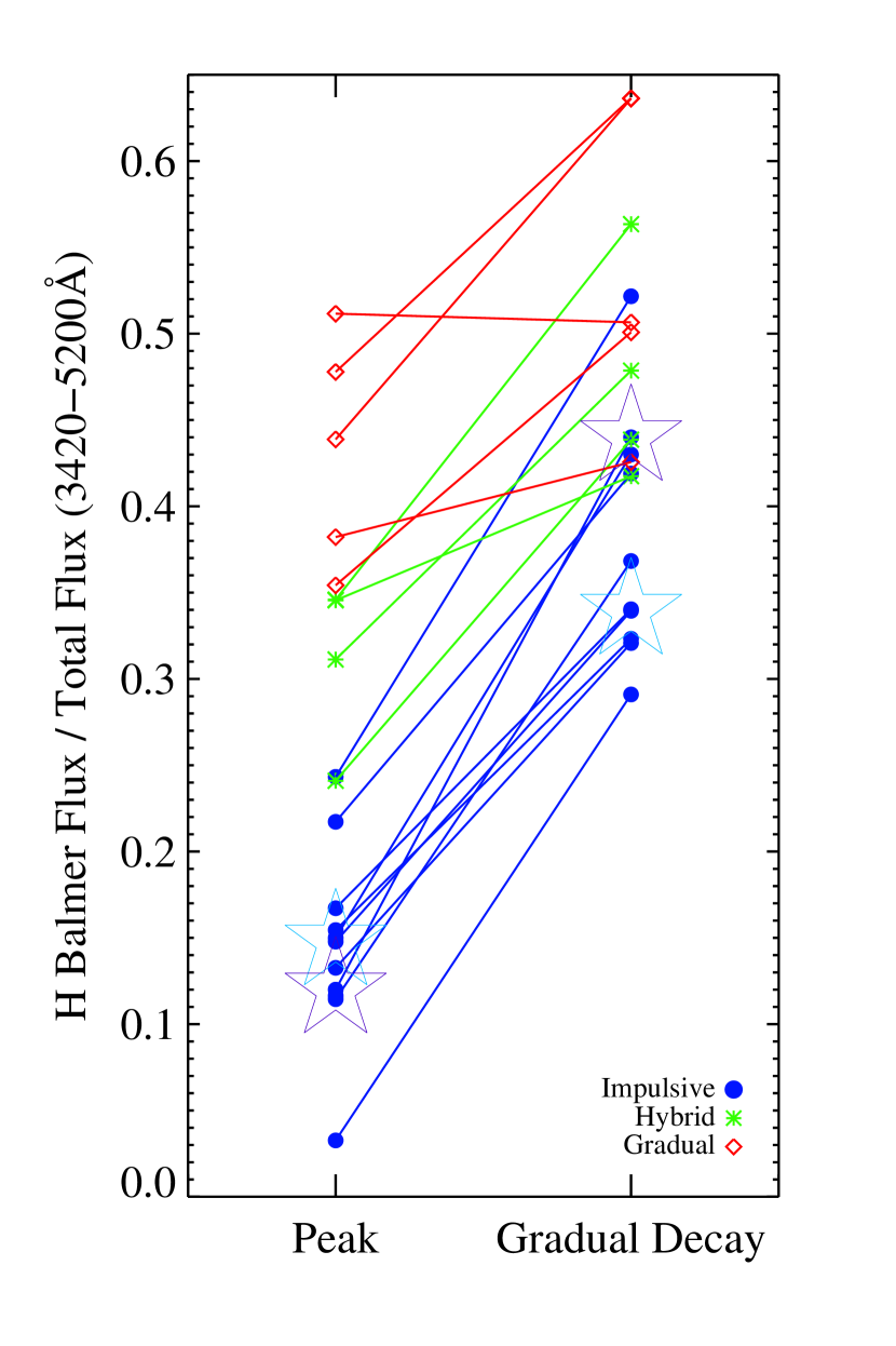
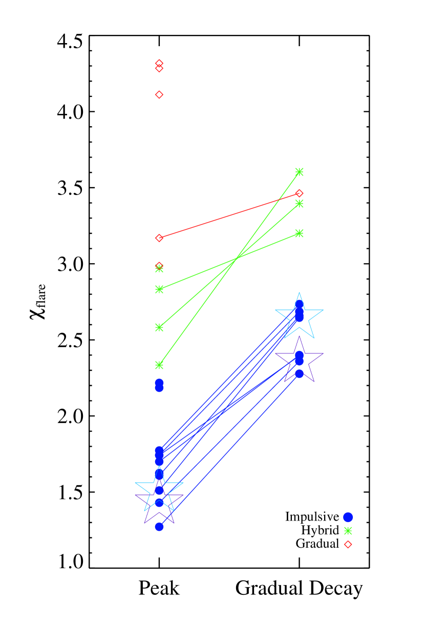
Figure 23: (Left panel) The relative contribution from the Hydrogen Balmer component during the peak and gradual phases. Light blue stars show the decay phase (S#23 – 25) and secondary flare (S#103) values for IF1; purple stars are the peak of the second continuum maximum ($t=1038$s, S#40) and the beginning gradual phase for the Great Flare (IF0). (Right panel) The evolution of $\chi_{\mathrm{flare}}$ from peak to gradual phases, calculated at the same times as in the panel to the left. The $\chi_{\mathrm{flare,decay}}$ values are not included if they have $>$20% errors (due to very low levels of emission in the decay phase). This cut excludes IF5, IF6, GF3, IF8, GF5, GF4, and GF2.

The Hydrogen Balmer (HB) component is the sum of the fluxes in H$\delta$, H$\gamma$, H$\beta$, the PseudoC, and the BaC (see Section 3.2). The HB component does not include H$\epsilon$ (H7) in the blue-optical because it is blended with Ca ii H, and it does not include H$\alpha$ because it is not available for some flares due to lack of wavelength coverage or saturated flux values (IF0, IF1, IF10, IF4, IF6, HF4, and GF3; see Kowalski (2012) for an analysis of the H$\alpha$ line evolution in the Flare Atlas). We investigate the coarse time-evolution of the percentage of HB flux (“%HB” or “HB flux ratio”) to total ($\lambda=3420-5200$Å) flare flux at the time of maximum continuum emission and near the beginning of the gradual decay phase (these times and spectrum numbers are given in Table 5 and are indicated by red vertical lines in Appendix B, Figures 43 – 61). The gradual decay phase measurements are averaged over three spectra, and the peak measurements are averaged in several of the GF events to increase signal-to-noise. The results are shown in Figure 23 (left panel) and given in Table 8 for the impulsive, hybrid, and gradual flares. The spectra S#23 – 25 (gradual decay) and #113 (just before peak of MDSF2) measurements are shown for IF1 as light blue star symbols and the IF0 peak and decay spectra are shown as dark purple star symbols.

Nearly every flare shows an increasing percentage of HB flux from the peak to the gradual decay phase, indicating that the gradual decay phase emission is marked by an increased relative importance of Hydrogen Balmer emission. The percentages increase by $\sim$20% for most flares; larger changes by $\sim$30% occur during IF0, IF3, IF4, IF5. Except for IF3, these flares also have very sudden breaks from impulsive to gradual phases. Significantly smaller changes, $<$20%, occur during HF3, GF1, and GF5 because the gradual decay phase of these flares begins at a relatively high amplitude compared to the peak, and the break from impulsive to gradual phases is much less defined.

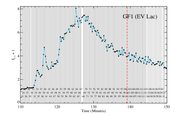
Figure 57: Same as Figure 43 but for GF1.

There is also an increasing percentage of Hydrogen Balmer emission during both the peak and decay phases according to the IF/HF/GF sequence, in agreement with the flux of H$\gamma$ divided by C4170 at peak emission in Figure 13. The impulsive flares show a range of 3 – 24% at peak, with most between 11 – 17%, but changing to $\sim 30-52$% during the gradual decay phase. The HF events are scattered around $25-35$% at peak and $40-50$% in the gradual decay phase, while the GF events are scattered around $35-50$% at peak and 40 – 65% in the gradual decay phase. The GF events show more scatter and less uniformity in their behavior compared to the IF and HF events. Note the light curve morphology of GF1 (Figure 57 of Appendix B); there are impulsive phases at $t\sim$1.92 hours, $t\sim 1.94$ hours, and $t\sim 2.02$ hours prior to the major, broad emission peak at $t\sim 2.13$ hours. The values in these peaks are $\sim$28%, 25%, and 36%, compared to 38% in the main peak.

The individual flux contributions from H$\delta$, H$\gamma$, H$\beta$  and H$\alpha$ are also given in Table 8 for the peak phases (maximum C3615) of each flare. The values for H$\delta$, H$\gamma$, and H$\beta$ also trace the morphological classification of a flare: IF events produce $<$1 – 2%, HF events produce $\sim$2 – 3%, and GF events produce 3% or more of the $\lambda=3420-5200$Å flux in each of these Hydrogen Balmer lines. When available, the flux contribution from H$\alpha$ is generally similar to the other Hydrogen lines at maximum continuum emission. The individual contributions are important constraints for RHD models that calculate the detailed radiative transfer using a relatively small Hydrogen atom (6 levels is typically used) and because blending from neighboring Hydrogen lines does not affect the flux measurements of the lower order transitions.

The evolution of $\chi_{\mathrm{flare}}$ (C3615/C4170) from the peak to the gradual phase times is shown in the right panel of Figure 23 and the values are given in Table 7. Indeed, both $\chi_{\mathrm{flare}}$ and the percentage of HB emission increase during the flare gradual decay phases, implying a connection between these measures. The IF events show rather similar trends: they have a change in the percentage of HB emission of $\sim 20-30$% and $\Delta$$\chi_{\mathrm{flare}}$$\sim$1 from the peak to the gradual decay phase times. The IF5 and IF6 events stand out as IF events that have a large amount of HB ($>20\%$) and large $\chi_{\mathrm{flare}}$ ($\sim$2.2) at peak (see also Section 4.3.1). These two flares have percentages of HB emission that rise to large values ($42-52$%) and values of $\chi_{\mathrm{flare}}$ that increase to $\sim$4 in the gradual decay phase, further strengthening the connection between these two measures ($\chi_{\mathrm{flare}}$, HB flux / total flux) even for the seemingly peculiar IF events that are not as similar as the other flares in the IF type.

The peak phase value of the percentage of HB emission for IF1/MDSF2 coincidentally falls within the same range as the other IF events; however, the percentage of the newly formed Balmer emission is uncertain due to Hydrogen Balmer absorption during this secondary flare (Section 6.3). The $\chi_{\mathrm{flare}}$ of IF1 for peak of MDSF2 and decay at the start of the spectral observations (light blue star symbols) are also consistent with the other IF events, even though a large amount of decay emission is present at the start of MDSF2.

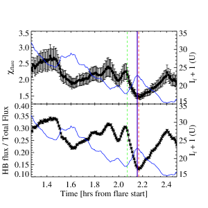
Figure 24: (Top Panel) The $\chi_{\mathrm{flare}}$ as a function time (black circles) and the $U$-band evolution (blue) are shown. (Bottom Panel) The time-evolution of the ratio of HB flux to total flux (dark asterisks). The ratio varies significantly and is anti-correlated with the $U$-band, strikingly similar to the evolution of $\chi_{\mathrm{flare}}$. The secondary flare, MDSF2, begins at $t\sim 2.072$ hours (vertical green line), peaks in the $U$ band between $t=2.1523$ and $t=$2.1587 hours (vertical purple line), and the minimum percentage of HB emission does not occur until slightly after the peak at $t=$2.1674 hours (vertical red line). Error bars on the bottom panel are the estimated statistical errors (not visible compared to the symbols). They assume that the uncertainties in the levels of the BaC flux and PseudoC flux are given by the difference in blackbody fits and straight line fits.

A time-resolved analysis of IF1 reveals the strong connection between the detailed evolution of $\chi_{\mathrm{flare}}$ and the percentage of HB emission during successive impulsive (e.g., MDSF2) and gradual decay phases. In Figure 24 (top), the $\chi_{\mathrm{flare}}$ evolution is compared to the $U$-band evolution over 1.3 hours of the decay phase of IF1. The trends are anti-correlated during the secondary flares with $U$-band peaks at $t\approx 1.6$ hours and $t\approx 2.16$ hours (MDSF2), as shown in Kowalski et al. (2011b). In Figure 24 (bottom panel), the percentage of HB emission is shown, and it varies similarly with $\chi_{\mathrm{flare}}$. The anti-correlated behavior between the percentage of HB emission and the $U$-band (blue) is very similar to that between the $U$-band and $\chi_{\mathrm{flare}}$. The maximum percentage of HB emission is 35%, but then drops to a minimum of 15% at $t\approx 2.17$ hours just after the $U$-band peak of MDSF2. The vertical line in both panels denotes the time of minimum percentage of HB emission (at S#116), which occurs just before the minimum $\chi_{\mathrm{flare}}$ and just after the maximum $U$-band enhancement. The time-differences between maxima and minima in $\chi_{\mathrm{flare}}$, percentage of HB emission, and the $U$-band are intriguing and should be confirmed with higher cadence data covering the peak and initial fast decay phase.

The percentages of HB flux in flares (Table 8, columns 2 and 3) should be directly compared to RHD models. The non-HB flux [1 – HB flux/total flux] is largely due to flux from the underlying white-light continuum that extends from the NUV through the optical. This accounts for the majority ($\gtrsim 50$%) of the total flux in all flares at peak, and as much as 83 – 89% of the total flux at peak in most IF events. For the first time, we have included the Balmer continuum at $\lambda>3420$Å in the energy budget with the other Balmer features, and we have shown that the Balmer component is not the dominant source of flux in flare emission in the blue. At most, the Balmer contribution accounts for $\sim$50% of the blue-optical flux, and only in gradual flares and the decay phase of other flares. The continuum component that accounts for the non-HB flux is represented by C4170. In the next section (Section 6), we will model this non-HB emission as hot, blackbody emission.

6 The Impulsive Phase Blue Continuum: Two-Component Analysis

The relative amount of each emission component as a function of time is important for understanding the distribution of flare heating in the stellar atmosphere. We extend the two-component continuum analysis from Kowalski et al. (2010) to the Flare Atlas and find that the blackbody and Balmer continuum components account for most of the NUV/blue continuum emission in both gradual and impulsive phases. In this section, we present the blue continuum properties of the flare peak emission. Note that “flare peak” and “maximum continuum” always refer to the times of maximum C3615 (see Section 3.2).

6.1 Flare Peak Blackbody Emission

In Section 4 (Figures  8  –  11), we showed the flare spectra at peak times for all flares. The flare peak spectra exhibit a steeply rising continuum towards NUV wavelengths, which is nearly ubiquitous and continues into the NUV beyond the spectral range of DIS. In Section 5.4, we found that typically only 11 – 17% of the flux from $\lambda=3400-5200$Å in the flare peak spectra of the IF events is accounted for by Hydrogen Balmer (line and continuum) emission (Figure 23). We find that the spectral shape of non-Hydrogen Balmer emission matches that of hot blackbody emission which pervades the entire NUV, blue-optical, and red-optical zones; C4170 is dominated by the emission from the blackbody continuum component.

The blackbody fitting is performed as follows. We calculate a color temperature, $T_{BB}$, of the blue-optical continuum by fitting a Planck function to the flux in the continuum windows from $\lambda=4000-4800$Å (BW1 – BW6, similar to those used in Kowalski et al. (2010)) given in Table 4. We used the peak flare spectrum from 2011 Feb 24 (IF3) and a decay spectrum from 2009 Jan 16 (IF1) to guide our selection of line-free regions. The same windows were used to fit a straight line to the continuum in order to calculate BaC3615 (Section 3.2). We do not include the flux at shorter wavelengths due to the difficulty in determining bona-fide continuum from blended Hydrogen lines (PseudoC) and due to the contribution from Balmer continuum emission. We do not include flux from redder wavelengths, because we find evidence for complicated behavior in the red-optical (Section 8). We also fit a filling factor ($X_{\mathrm{BB}}=R_{\mathrm{fl}}^{2}/R_{\mathrm{star}}^{2}$; as in Hawley et al. (2003) and Kowalski et al. (2010)) using the IDL routine mpcurvefit, where $X$ is the fraction of the visible hemisphere covered by the projected area of the flare (discussed in Section 10.1). The two parameters are fit simultaneously, which is an important distinction to the analysis from Kowalski et al. (2010) where $T_{\mathrm{BB}}$ was fixed to $9\,000$ K, $10\,000$ K, and $11\,000$ K. The fits for IF1 are redone here using the new flux scaling (Section 2.6), and some quantities change compared to those in Kowalski et al. (2010, 2012). Good quality fits are obtained for the IF events (except for IF6), the HF events, GF1, GF3 and GF5.

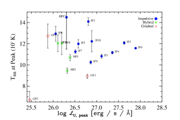
Figure 25: The distribution of $T_{\mathrm{BB}}$ at the time of maximum continuum (C3615) emission vs. the peak specific $U$-band luminosity for the seventeen flares with well-determined color temperatures.

The blackbody fits are indicated by light blue lines in the flare peak spectra panels (Figures  8  –  11) and are given in parentheses. In Figure 25, we show the distribution of $T_{BB}$ at maximum continuum emission for the seventeen flares with well-determined temperatures (values are given in Table 7). The flares are colored by the morphological type, but there is no discernible trend with type or peak $\mathcal{L}_{U}$. We find that $T_{\mathrm{BB}}=10\,000-14\,000$ K for the IF events (Figure  8). By comparing to the dotted (pre-flare) spectra we see that this hot, blackbody component is present for a variety of flare amplitudes, appearing in flares with peak $U$-band enhancements greater than $I_{f,U}+1\sim$3, and as large as $I_{f,U}+1\sim$80. The high signal-to-noise ratio of our spectra makes the characterization of this component possible even with relatively small contrast in the blue-optical at $\lambda>4500$Å. The blackbody component contributes $\sim 76-97$%, and on average 84%, of the $\lambda=3420-5200$Å flux during the peak times for the IF events (Section 5.4).

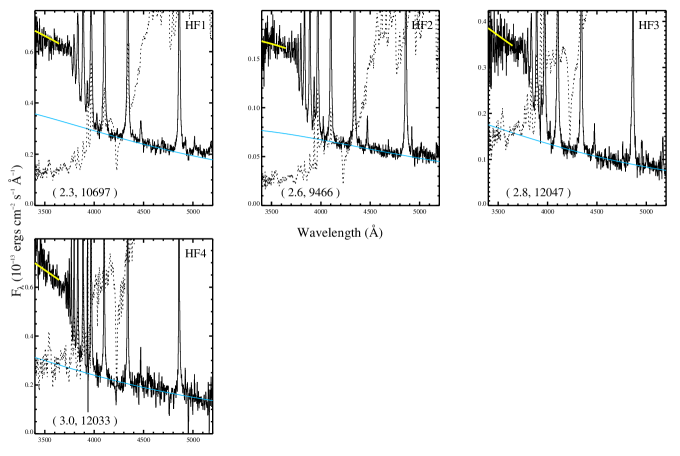
Figure 10: Same as in Figure 8.

The flare peak spectra of the HF events (Figure 10) also show the hot, blackbody component, with temperatures between $T_{\mathrm{BB}}$$\sim 9500-12\,000$ K. The lower amplitudes of these flares are noticeable, e.g., by comparing to the pre-flare spectra. The HF events also have a conspicuous amount of excess emission above the extrapolated light blue curve at $\lambda<3800$Å. Of the GF events in Figure  11, the large-amplitude, high energy gradual flare GF1 shows the most convincing evidence of a moderately hot blackbody, with $T_{\mathrm{BB}}$$\sim 9000$ K. A significant NUV excess is also present during this flare. GF1 has a small-amplitude impulsive phase with a strong response in C4170 that occurs before the main flare peak (see Figure 19); the newly formed flare emission in this pre-cursor flare peak has $T_{\mathrm{BB}}$$\sim$$14\,500$ and is included in Figure 25 as GF1^′. GF3 shows evidence of a high temperature, but these data have a more uncertain calibration; however, we averaged three spectra near the peak and derived a similar value of $T_{\mathrm{BB}}$ for this flare. We have averaged four spectra at the flare peak of GF5, which results in a relatively good fit, but with a lower temperature of $T_{\mathrm{BB}}$$\sim$6700 K. In GF2 and GF4, we cannot accurately ascertain the characteristics of the slope of the continuum; nonetheless, the very low-amplitude flares ($I_{f}+1\sim 1.3-2.2$, $|\Delta U|<1$ mag; GF2  –  GF5) do show excess C4170 emission.

The $\sim$5% blue-continuum shape uncertainty coupled with the uncertainty in the scale factor, $R$ (see Section 2 here and Appendix A of Kowalski (2012)), and also the contamination of continuum windows from emission lines (Hydrogen Balmer line wings and low-level Fe and Ti lines) lead to systematic uncertainties in the blackbody temperatures of about $500-1200$ K. The statistical uncertainties are only $\sim$200 K for most events, and are indicated by the error bars in Figure 25. Kowalski et al. (2010) found a $\pm 1000$ K range in temperatures that well-represented the blue continuum shape. In Appendix F of Kowalski (2012), the detailed systematic errors involved with temperature fitting are examined. The important result is that for the IF2 event, the extreme amount of line broadening causes the BW1 and BW2 fitting windows to have possible contamination from Balmer line wing emission; the acceptable range of $T_{\mathrm{BB}}$ for this flare is therefore $11\,700-14\,100$ K, however, the temperature of $14\,100$ K better accounts for the shape of the total emission in the BaC at $\lambda\lesssim 3646$Å.

In summary, we observe a continuum at flare peak times of the impulsive phase with a spectral slope matching that of a hot, blackbody with $T_{\mathrm{BB}}$$\sim$$9\,000-14\,000$ K (most within $10\,000-12\,000$ K) which is relatively independent of flare amplitude over a large range of peak $U$-band specific luminosities, total energies, and light curve morphologies. For this range of temperatures, the spectrum would not be expected to strictly follow a $\lambda^{-4}$ slope according to the Rayleigh-Jeans law. Instead, a linearly decreasing fit to the blue optical zone gives a reasonably good fit and looks very similar to a Planck function for these temperatures: in the formula for the Planck function, the steeply decreasing $\lambda^{-5}$ part multiplies with the increasing exponential part, giving a linear decrease towards the red for $\lambda=4000-5000$Å.

The interflare variation in $T_{\mathrm{BB}}$ at flare peak is likely significant despite the large systematic uncertainties of $\sim$1000 K. We show convincing evidence that interflare variations are significant between two flares, IF2 and HF1, in Appendix G, and we discuss the implications for flare heating differences in Section 11. Additional high signal-to-noise data would be useful to determine if the color temperature decreases to $\sim$7000 K at flare peak during very small amplitude events ($I_{f}+1\lesssim 1.5$), as implied by the observations of GF5. NUV data covering the flare peak of the continuum (likely near $\lambda=2500-3000$Å) would help to more precisely determine the blackbody temperature at flare peak and its evolution during the impulsive phase.

This hot, blackbody continuum component has been detected previously using colorimetry and spectra (see references in the Introduction). Self-consistent flare heating models of the impulsive phase have thus far not reproduced this (dominant) emission component; we compare to current models in Section 9. In summary, we have found that a $T_{\mathrm{BB}}$$\sim 10^{4}$ K blackbody function and linear function are useful mathematical representations for this continuum component; however, we will shortly show (Section 6.3) that a single blackbody or line does not account for important absorption features in the spectrum.

6.2 Flare Peak Balmer Continuum Emission

We find that there is always excess flux in the NUV zone, above an extrapolation of the Planck function at these wavelengths. The slope of the total NUV spectral zone emission at flare peak generally follows the same slope as the underlying Planck function. In Figures 8  –  11, we scaled the Planck function to the flux at C3615, and showed in yellow that it matched the flux at $\lambda<3646$Å, illustrating that the overall shape of the continuum at $\lambda<3646$Å for the IF, HF, and some GF events can be represented by about the same temperature fit as for the blue-optical. We measure the slope of the NUV flare emission at $3420\leq\lambda\leq 3630$Å by fitting a line to three wavelength bins in this region. These values are given in Table 7 (columns 9 and 10 are the values for the flare peak and gradual decay phase; columns 11 and 12 are the values for the flare peak and gradual decay phase with the underlying blackbody emission subtracted) are consistent with the blue spectral shape indicated by the yellow curves, and will be important for comparing to detailed Balmer continuum model predictions in Section 9. Note, the flux calibration errors in the NUV are larger ($\sim$5 – 10%), and the statistical uncertainties in the fits can also become comparatively large; higher signal-to-noise measurements should be obtained in the NUV.

Although the total flux at $\lambda<3646$Å follows the same general slope as the underlying blackbody, we attribute the excess flux in the NUV to chromospheric Balmer continuum (BaC) radiation from recombination to the $n=2$ level of Hydrogen, as in Kowalski et al. (2010). We find that Balmer continuum emission is ubiquitous at flare peak for all flares in our sample, consistent with our conclusion that Balmer continuum emission affects the value of $\chi_{\mathrm{flare,peak}}$ and is correlated with the relative amount of H$\gamma$ emission (Section 4.3.1, Figure 13). As explained in Section 3.2, we use both the BaC3615 and BaC quantities as measures of the Balmer continuum emission.

In Figure 26, we show BaC3615/C3615 (the fraction of the NUV flux emitted in Balmer continuum emission) and find a general ordering between the IF, HF, and GF events. There is a decreasing trend with peak specific $U$-band luminosity with a range of values for each morphology class, especially for the IF events, which have a standard deviation that is twice the standard deviation of the percentage of HB emission (Section 5.4). The IF events are least dominated by BaC3615 with most having values of 0.2  –  0.35. These flares are dominated by the hot blackbody emission component which also contributes to the flux of C3615. While the IF5 and IF6 events have larger values, $\sim$0.4, IF4 has a very low value $\sim$0.05 (but also required additional calibration – see Appendix A of Kowalski (2012)). The HF events have about equal contributions ($\sim$0.5  –  0.6) and the GF events have the majority of their peak NUV flux (0.55  –  0.8) in Balmer continuum emission. In column 8 of Table 8, we present these values. We conclude that the general relationship is that the overall light curve evolution (flare morphology) is physically connected to the relative importance of the Balmer continuum flux at the time of maximum continuum emission.

6.3 An “A star” on an “M star”: Absorption Features in Flare Spectra

Several flares in our sample have impulsive phase durations that are significantly longer than the spectral cadence, thereby allowing detailed time-resolved analyses of the two continuum components. In particular, IF1, IF3, and GF1 have the greatest number of spectra during their respective impulsive phases (see Figures in Appendix B). Note that the impulsive phase of IF1 refers to the subpeak MDSF2, not the main flare peak which did not have spectral coverage.

In this section, we analyze the rise phase and peak spectra of MDSF2, to show that the hot, blackbody continuum component is not a featureless Planck function across our wavelength range. Here, we establish the presence of absorption features in impulsive phase flare emission, and thereby redefine how we understand the “blackbody” continuum properties (e.g., Figure 25).

An indication for the presence of absorption in our spatially unresolved flare data is an anti-correlation between the time-evolution of BaC3615 and the time-evolution of the total amount of the blue/NUV continuum, as diagnosed by the $U$-band flux or C$4170$ flux. This effect has been observed during the secondary flares in the decay phase of IF1 (Figure 1d of Kowalski et al., 2010) and presented graphically through a sequence of rise-phase spectra (Figure 1 of Kowalski et al., 2012). Those figures illustrate that as the $U$-band increases during the secondary flare MDSF2, the entire blue/NUV continuum becomes dominated by the blackbody component whereas the absolute (and relative) amount of BaC3615 decreases.

In previous papers on IF1/MDSF2 (Kowalski et al., 2011a, 2012), we have denoted the sum of all (spatially unresolved) decaying and impulsive flare emission as $F_{\lambda}^{\prime}$ (obtained by subtracting the preflare quiescent spectrum), and newly-formed flare emission isolated from an impulsive event as $F_{\lambda}^{\prime\prime}$ (obtained from subtracting the preflare decaying emission). During MDSF2, we find direct evidence that the newly-formed flare emission ($F_{\lambda}^{\prime\prime}$) during the rise phase resembles the spectrum of a hot star. This was first shown in Kowalski et al. (2011a); in this section, we present an analysis of the time-evolution.

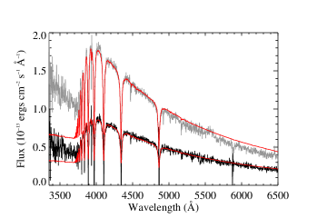
Figure 27: The black is the newly-formed flare emission approximately half way up the rise of the secondary flare MDSF2 (an average spectrum of S#108 and S#109) and the grey is the newly-formed flare emission just prior to the sub-peak (S#113). The red is the spectrum of Vega with a scaling applied to match the flare spectra at C4170.

Figure 27 shows the newly-formed flare spectra ($F_{\lambda}^{\prime\prime}$) during the rise (black; same spectrum as presented in Kowalski et al. (2011a)) and just prior to the sub-peak (grey) at $\lambda<6500$Å. At both times, the blue-optical shapes are well-matched by the spectrum of Vega (from Bohlin, 2007) scaled and plotted in red to show the striking similarities in the spectral slope and absorption features. The difference between the flux at $\lambda<3600$Å in the grey spectrum and the flux in Vega could be due to the spatially unresolved chromospheric Balmer continuum emission forming during the event or due to the difference in gravity between the hot star and an M dwarf (log $g=4$ and log $g=5$, respectively). Models of deep heating (e.g., Kowalski et al., 2011a) in M dwarfs are required to understand these detailed spectral differences.

Mihalas (1970) discusses the detailed formation of hot-star spectra: The lower emission at $\lambda\sim 3615$Å relative to the emission at $\lambda\sim 4170$Å (in other words, the BaC is in absorption) is a result of the non-uniform temperature structure of the atmosphere coupled with wavelength dependent Hydrogen Balmer and Paschen continua opacities (and flux redistribution) in an optically thick medium. In other words, the optically thick emitting material producing the $\lambda\sim 3615$Å emission is at a lower temperature (e.g., from lower column mass or higher height for a radiative equilibrium stratification) than the optically thick emitting material at $\lambda\sim 4170$Å. We have therefore revealed the multithermal contributions that comprise the hot blackbody emission component (see Section 6.1 and Figure 25). The use of the blackbody function (and $T_{\mathrm{BB}}$) is a useful paramaterization of the $\lambda=4000-4800$Å slope, but it is important to realize that it is an approximation of the detailed radiation field originating from a flare atmosphere with an opacity dependence as a function of wavelength and a temperature dependence as a function of height.

Temperature evolution during the rise of MDSF2 is qualitatively evident in Figure 27 by comparing the blue-optical spectral shape to Vega from flare rise (black) to flare peak (grey). The spectrum becomes steeper (corresponding to a hotter color temperature), and there are three ways to measure this for any given time during MDSF2. For example, we consider the spectrum near maximum continuum emission (S#113, the grey spectrum in Figure 27):

1. Method 1: Color temperature of total flare-only emission: The color temperature of the total emission with quiescent level subtracted ($F_{\lambda}^{\prime}$) is $\sim$$11\,000$ K (Figure 25). This represents the color temperature averaged over the entire flaring area over the duration of the exposure (Kowalski et al., 2012).

2. Method 2: Color temperature of newly-formed flare-only emission: The temperature of the newly-formed flare emission ($F_{\lambda}^{\prime\prime}$) is $\sim$$18\,000$ K just prior to the $U$-band peak. This temperature is obtained by subtracting the previously quiescent$+$decay flare emission. This technique provides a better estimate for the shape of the continuum that is produced during the times when there is a secondary impulsive flare event. Relating the continuum shape to a color temperature with this technique assumes that the 1) the previously decaying emission is small or that it does not decay significantly and 2) the newly-formed flare emission originates from a spatially distinct flare area that was not previously heated. Otherwise, the non-linear dependence between $T$ and intensity (e.g., for the Planck function) results in an incorrect association between $T_{\mathrm{BB}}$ and $F_{\lambda}\prime\prime$.

3. Method 3: Adjusted color temperature of newly-formed flare-only emission: In Appendix D, we estimate the amount by which the flux of the previously decaying emission has decreases during the secondary flare. We apply these estimates to the times of the spectra during MDSF2 which allows the best derivation of the properties of the newly-formed flare emission. We find that the color temperatures are $\sim$1800 – 2700 K lower than method #2 (above). The value at flare peak of MDSF2 ($T_{\mathrm{BB}}$$\sim$$15\,000$ K) falls just beyond the high end of the sample’s distribution of $T_{\mathrm{BB}}$ in Figure 25.

We summarize the derived color temperature values at three times in Table 9 using these three methods. The times correspond to the time just before MDSF2, halfway through the rise phase of MDSF2, and just prior to flare peak of MDSF2. The observed, apparent anti-correlation between the time evolution of Balmer continuum emission (BaC3615) and blackbody emission (Kowalski et al., 2010, 2011b, 2012) is now explained by the presence of an emission component with “absorption” features forming during the flare. If there are significant absorption components in other flares, then the value of the derived BaC3615 value for these flares (obtained from a linear extrapolation – see Section 3.2) is an underestimate of the intrinsic amount of Balmer continuum emission originating from the chromosphere.

We briefly examine whether Balmer continuum absorption has an obvious effect on the distribution of the peak properties of the Flare Atlas. We calculate the peak specific luminosities of C4170 and BaC3615 (see Sections 3.1, 3.2). We find that in general, the IF events (with lower $\chi_{\mathrm{flare,peak}}$ values; Section 4.3.1) are more luminous in C4170 whether the BaC3615 is emission or absorption (on average, $\mathcal{L}_{\mathrm{C}4170}/\mathcal{L}_{\mathrm{BaC}3615}=2.4$), the GF events are more luminous in BaC3615 (on average, $\mathcal{L}_{\mathrm{BaC}3615}/\mathcal{L}_{\mathrm{C}4170}=2.4$) and the HF events are slightly more luminous in BaC3615 (on average, $\mathcal{L}_{\mathrm{BaC}3615}/\mathcal{L}_{\mathrm{C}4170}=1.5$) . The trend between morphological type and the relative amounts of BaC3615 and C4170 could be related to the amount of BaC absorption produced by the blackbody (C4170) component. Since the amount of BaC3615 that we measure is probably less than the intrinsic BaC3615 emission (due to this absorption component) the emission and absorption may add together to produce smaller values of BaC3615 – and $\chi_{\mathrm{flare,peak}}$– for the IF events. The HF and GF events may produce intrinsically more BaC3615 than the IF events, they may produce less BaC3615 absorption than the IF events, or they may have both effects. However, we suggest the possibility that absorption can also lead to both low values of $\chi_{\mathrm{flare,peak}}$ and large values of C4170/BaC3615. The Balmer continuum emission produced in large amounts in the early flare phases, and persisting over a relatively long time compared to the blackbody component, effectively veils the absorption signatures except in the flares with the most extreme heating. Detailed modeling of the blackbody component over a large parameter space is needed to understand the role of absorption in flares of all morphological types.

6.4 Balmer Wing Absorption

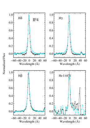
Figure 28: The H$\delta$, H$\gamma$, H$\beta$ and He I $\lambda$4471 profiles of IF4 at peak continuum emission (S#665, black) and peak H$\beta$ emission (S#672, turquoise), normalized to the maxima of the line profiles. A fit to the local continuum was removed before normalization. For H$\delta$, H$\gamma$, and H$\beta$ respectively, the widths are (15.5Å, 16.7Å, 21.4Å) at maximum continuum and (21.8Å, 22.6Å, 23.7Å) at maximum line emission. The maximum line emission occurs at the same time for the three lines, $\sim$4.5 minutes after the maximum continuum emission. The feature at $+40$Å in the He i panel is likely a cosmic ray. We attribute the deficit in flux at $\pm$20Å in the black spectrum, which is especially apparent around H$\delta$, to the formation of A-type star absorption wings during the flare.

We now present cases of line broadening in larger flares where there is evidence of absorption in the wings. In Figure 28, we show H$\delta$, H$\gamma$, H$\beta$, and He i $\lambda$4471 profiles ($F_{\lambda}^{\prime}$) for IF4, at maximum continuum emission (black, S#665) and at maximum Balmer line emission (S#672, turquoise). The profiles are plotted with the local continuum subtracted with a straight line and then are normalized to the peak of the line. The striking effect here is a “depression” (deficit) in the line wings in the black profile (maximum continuum) between $\pm 10$Å to $\pm 30$Å from line center. Furthermore, the amount of wing depression increases from H$\beta$ to H$\delta$. The differences in the widths (measured at the 10% line flux level) between the times of maximum continuum flux and maximum line flux are $\sim$6Å for H$\delta$ and H$\gamma$ and $\sim$2Å for H$\beta$. Although the change in the line widths for H$\delta$ and H$\gamma$ are just $\sim$2$\sigma$ (from 3Å uncertainty in widths), we observe a flux depression (deficit) over at least 10 contiguous pixels in the wings on both sides of the line center, which increases the significance of the flux depression. During the rise phase spectrum (S#664, corresponding to a flux of $\sim$40% of the peak continuum emission), the Balmer lines are narrower than at both maximum line and continuum emission, but there is less evidence for flux depressions in the line wings. In the spectrum following flare peak, the Balmer lines have begun to broaden significantly and no wing depressions are seen.

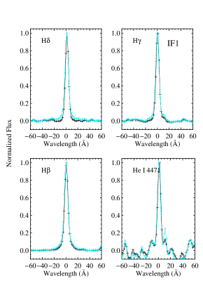
Figure 29: The H$\delta$, H$\gamma$, H$\beta$ and He I $\lambda$4471 profiles of IF1 at peak continuum of MDSF2 (S#113, black) and peak H$\beta$ emission (S#24, turquoise), normalized to the maxima of the line profiles. A fit to the local continuum was removed before normalization. In the peak continuum spectrum, the line wings are depressed relative to the nearby continuum level, the depressions are more apparent for the higher order lines, and the line widths are smaller. These effects are similarly seen in IF4 (Figure 28). The widths of H$\delta$, H$\gamma$, and H$\beta$ are 12.2, 12.6, and 15.2Å at maximum continuum emission and 14.8, 14.9, and 18.2Å at maximum line emission. The feature at $+10$Å from Helium is likely Mg ii $\lambda$4481.

A similar wing depression effect is seen in the IF1 spectra during the peak continuum emission of the subpeak MDSF2. In Figure 29, we show the profiles for the IF1 flare near the time of maximum Balmer line emission within the spectral observation window (turquoise) and at the peak continuum emission (black) during MDSF2. The wing depression is present, but relatively less than in IF4 (Figure 28), and doesn’t appear as far from line center as in IF4. The wing depression increases for the higher order Balmer lines as in IF4. The line widths (measured at the 10% line flux level) at the time of maximum continuum emission are 2 – 3Å narrower than at the time of maximum line emission.

We find similar evidence for wing depressions during flare peak of IF3 (see Appendix E), given that the rise phase emission is subtracted from the flare peak.

For IF1, the newly formed flare emission during MDSF2 was found to have a spectrum like a hot star, with the Balmer lines in absorption (see Section 6.3). In particular, note the similarities in the widths of the Balmer absorption lines between the Vega spectrum and the flare spectra in Figure 27. We therefore interpret the wing depressions in IF1 and IF4 as direct signatures of Balmer line absorption forming during these flares. The absorption wings in model hot star spectra with log $g=4-5$ are very broad (Castelli & Kurucz, 2004) due to Stark broadening (Peterson, 1969). The superposition of an emission line component and an absorption line component leads to the net decrease that we observe in the wings in the flare spectra. As a result of the superposition of emission and absorption, the measured line widths (at the 10% flux level) also decrease. The Balmer absorption line flux decrement for Vega is H$\delta$ : H$\gamma$ : H$\beta$ $\approx 1.09:1.00:0.75$ (using the spectrum from Bohlin, 2007); therefore, one would expect the line widths and wing fluxes of the higher order Balmer lines in flare spectra to be more strongly affected in the presence of hot star-like absorption. The Balmer emission line component originates from the flaring chromosphere (Hawley & Fisher, 1992; Allred et al., 2006) and veils the Balmer absorption component in the total, spatially unresolved flare spectrum. See Johns-Krull et al. (1997) for a phenomenological illustration using quiet-Sun H$\alpha$ absorption and superimposed chromospheric H$\alpha$ emission.

Wing absorption signifies heating in deep layers of the atmosphere, which is an important constraint for flare heating models. The heating differences between flares - e.g., between the primary flare of IF4 and the secondary flare MDSF2 - should be studied with radiative-hydrodynamic models that successfully produce the range of blackbody continuum properties. These flares have two of the three lowest $\chi_{\mathrm{flare,peak}}$ values in the sample ($\chi_{\mathrm{flare,peak}}$$\sim$1.3 – 1.5; Table 7) and also show evidence of Balmer line wing absorption, implying a common heating scenario. Further, the data are suggestive of differences in $\chi_{\mathrm{flare,peak}}$ and the amount of Balmer line wing absorption (IF4 having a smaller $\chi_{\mathrm{flare,peak}}$ and also more wing absorption, as is most evident for H$\delta$). Also, the peak $U$-band amplitude is much larger in IF4 ($I_{f,U}$$\sim$20) than in MDSF2 ($I_{f,U}$$\sim$7). Assuming that IF4 produced the same type of “blackbody” emission as MDSF2 (Section 6.3) with $T_{\mathrm{BB}}$$=$15 000 K (Table 9), the inferred area of this emission would be over 3 times as large in IF4 and formed over a timescale nine times as fast ($t_{1/2,\mathrm{C4170}}\sim 1$ min for IF4, $t_{1/2,\mathrm{C4170}}\sim 9$ min for MDSF2; Table 7). As a result, more “blackbody” emission formed over less time leads to more obvious absorption wings at peak. On the other hand, it is possible that the “blackbody” emission is intrinsically different between the two flares, related to the speed at which the light curve develops and ultimately to the depth of primary heating (IF4) compared to the depth at which primary heating (IF1) may cause secondary flare heating (MDSF2; see Section 10.2). It may also be important to consider that $I_{f,U}$ is much higher  –  therefore with more blackbody emission present  –  in the maximum line emission spectrum for IF1 ($I_{f,U}$ $\sim$35 at S#24) than for IF4 ($I_{f,U}$ $\sim$4 at S#671).

Searching for wing depressions is a method for directly detecting hot star signatures in $F_{\lambda}^{\prime}$, without needing to isolate newly formed emission, a technique that relies on several assumptions (Section 6.3). This analysis can be employed with other flare data that cannot be accurately flux-calibrated, or for spectral data with limited wavelength range. A larger sample of primary and secondary peaks during high energy flares with high time resolution would be useful for constraining the timing of the absorption wings during the flare and also the relationship between a very small value of $\chi_{\mathrm{flare,peak}}$ $\sim$1.5 and the presence of absorption wings.

7 The Gradual Decay Phase Continuum

The gradual decay phase begins when the flare light curve transitions from a slow decay after the initial fast decay phase, marked by either a distinct break (e.g., IF4 or the $g$-band light curve of IF5) or a smooth transition into slowly decaying emission (e.g., IF2 and IF7). The $U$-band has typically reached $\sim$50% of the peak flux in the GF events and $10-20$% of the peak flux in the IF events at the start of the gradual decay phase.

In dMe flares, the gradual decay phase is energetically important due to its long duration. In IF0, 29% of the total $U$-band energy is emitted during the gradual decay phase (HP91). Over 70% of the $U$-band energy in IF1 and 60% of the $u$-band energy in IF3 were emitted in the gradual phases, giving a range of values even for flares of the same type. In Figure 23, we found that only $30-65$% of the wavelength-integrated flux at the beginning of the gradual decay phase can be attributed to Hydrogen Balmer radiation. Given that Ca ii, the Helium i lines, and various metal lines including Fe ii lines only account for $\sim 5$% of the emission, this leaves $30-65$% of the gradual phase emission due to non-Hydrogen Balmer radiation. According to Table 8 (column 9), $\sim 60$% of the specific flux in C3615 is due to the BaC3615 contribution, leaving $\sim$40% of the specific flux in the NUV unaccounted for by Balmer continuum emission.

Studies of the gradual decay phase continuum during IF1 were presented in Kowalski et al. (2010, 2012). A two-component model consisting of a $T_{\mathrm{BB}}$$=10\,000$ K blackbody and a RHD model Balmer continuum was used to derive a filling factor ratio ($X_{\mathrm{BaCF11}}/X_{\mathrm{BB}}$) of $\sim$$3-16$. The IF1 gradual decay phase showed direct evidence for a Balmer continuum in emission, which matched the RHD prediction from Allred et al. (2006). Thus far in the analysis of the Flare Atlas, we have seen that the Balmer jump ratio ($\chi_{\mathrm{flare}}$) and the percentage of flux that can be attributed to the Hydrogen Balmer (HB) emission increases in the gradual decay phase (Figure 23), indicating a change in the underlying radiative energy release processes. An important step in understanding the gradual decay phase flare heating includes determining if the gradual decaying continuum is due to the long cooling timescale (Cully et al., 1994) of material that was heated impulsively in the beginning of the flare, or if it is due to prolonged, low-level heating leading to cooler temperatures than in the beginning of the flare. If there is prolonged heating, then we must determine the source (e.g., particle heating, backwarming).

7.1 Gradual Decay Phase Spectra

To study the gradual phase, we average three spectra at the times given in Table 5 in order to increase the signal-to-noise in the blue-optical zone for determining a blackbody temperature fit. Figures 30 – 35 show the averaged spectra from the beginning of the gradual phase (Table 5 and indicated by vertical red lines in Appendix B, Figures 43 – 61) for flares with sufficient signal-to-noise for analysis. Note that IF4, IF5, and HF4 have only a single spectrum shown because the data quality was variable during the low levels of gradual phase emission. Two component fits, allowing $T_{\mathrm{BB}}$, $X_{\mathrm{BB}}$, and $X_{\mathrm{BaCF11}}$ to vary, are shown in color with the quiescent spectrum as a dotted line. The gradual phase spectrum for IF10 is given as S#32 even though it contains contributions from (relatively low level) secondary flares. In parentheses, we have listed $\chi_{\mathrm{flare,decay}}$ and $T_{\mathrm{BB}}$; the values are excluded when they are not well-determined (i.e., very little or no continuum emission in the blue-optical zone). We remind the reader that $T_{\mathrm{BB}}$ is a parametrization of the continuum slope; detailed modeling is required to deduce the multithermal structure of the atmosphere (see discussion in Section 6.3).

A striking similarity among the gradual phase spectra is the value of $T_{\mathrm{BB}}$, $\sim$7300 – 8500 K (typically around 8000 K) in the flares IF1, IF2, IF3, IF7, IF9, IF5, GF1, and HF2. However, some flares have unusual characteristics. The gradual phase of IF4 was taken near the peak of the line emission (due to the uncertainty in flux calibration later in the flare at very high airmass), and this flare has a larger color temperature of 9500 K. The gradual phases of HF1 and HF3 are also hotter with temperatures exceeding $10\,000$ K. We have averaged the spectra just following the peak (synthetic $U$-band) emission of GF5 to show the remarkable detection of white-light continuum (and all the typical flare emission lines) in an event with only $I_{f}+1<1.5$ and $I_{C4170}+1\sim$ 1.03. This flare has a gradual phase $T_{\mathrm{BB}}$$\sim$4900 K, the lowest detected temperature in our sample, and is about 2000 K cooler than at peak.

Note that the gradual phase spectrum of IF1 (Figure 30) is that shown in Figure 1b in Kowalski et al. (2010), where we modeled this spectrum with a $T=9\,000-11\,000$ K blackbody. $T_{\mathrm{BB}}$$\sim$8250 K results with our current, better determined fit, with a larger inferred areal coverage, $X_{\mathrm{BB}}$$\sim$0.4% of the visible hemisphere ($\sim$2 times the value given in Kowalski et al., 2010). Among the three spectra averaged to form the gradual phase spectrum of IF1 in Figure 30, the inferred temperature range is between 8000 – 8500 K. The difference between 8250 K and $10\,000$ K is significant, as our estimate of the systematic uncertainty in the temperature determinations is $\sim$1000 K (Kowalski, 2012, Appendix F).

We calculate the specific luminosities of BaC3615 and C4170 (see Sections 3.1, 3.2) and find a trend among the IF events showing $T_{\mathrm{BB}}$$\sim$8000 K emission in the gradual decay phase and $\chi_{\mathrm{flare,peak}}$$<$ 2: IF1, IF2, IF3, IF7, and IF9. These flares are described by the relation,

$$\mathrm{log_{10}}\mathcal{L}_{\mathrm{BaC3615}}=-0.63(\pm 0.86)+1.03(\pm 0.03)\times\mathrm{log_{10}}\mathcal{L}_{\mathrm{C4170}}$$ (9)

A slope of $\sim$1 indicates that the BaC3615 and C4170 specific luminosities increase in equal percentages during the gradual decay phase according to the size of the flare. The flares with $\chi_{\mathrm{flare,peak}}$ $>2$ and which form a $T_{\mathrm{BB}}$$\sim$8000 K component at the beginning of the gradual decay phase – IF5, HF2, and GF1 – may comprise a second distribution which is offset from those with $\chi_{\mathrm{flare,peak}}$ $<2$ and $T_{\mathrm{BB}}$$\sim$8000 K in the gradual decay phase. However, it is not clear whether the distribution is offset horizontally (signifying that they are “deficient” in C4170) or vertically (signifying that they have excess BaC3615). In any case, the data suggest that the persistence of C4170 with $T_{\mathrm{BB}}$$\sim$8000 K formation is related to the formation of BaC3615 in the gradual decay phase.

The $\chi_{\mathrm{flare}}$ value is approximately constant in the gradual decay phases of IF3 and GF1 ($\chi_{\mathrm{flare,decay}}$$\sim$2.7 and 3.5, respectively). What can we learn from this? This may indicate that the Hydrogen BaC and the C4170 – and therefore the $T_{\mathrm{BB}}$$\sim$8000 K blackbody component – vary together during the gradual decay phase. However, the interpretation of $\chi_{\mathrm{flare}}$ is complicated because variations in both the blackbody and BaC components can lead to variations in C3615, and therefore the value of $\chi_{\mathrm{flare}}$. For IF3, we investigate the ratio of BaC3615 to C4170. This ratio is similar to the evolution of $\chi_{\mathrm{flare}}$ for the duration of the flare, with both measures being relatively constant over $\sim$0.6 hours of the gradual phase. Because BaC3615/C4170 is nearly constant with values of $\sim$1.5 – 1.6 over this time period, we conclude that the local flux in the BaC at $\lambda=3615$Å does follow the local flux in the blackbody at $\lambda=4170$Å during the gradual phase.

In summary, we find evidence for a $T_{\mathrm{BB}}$$\sim$8000 K component at the beginning of the gradual decay phase during eight flares, most of which are IF events. It is not known if the emission is formed in the same areal region as the impulsive phase emission (with $T_{\mathrm{BB}}$$\sim$$9000-14\,000$). We find a strong correlation among different flares between the C4170 ($T_{\mathrm{BB}}$$\sim$8000 K) specific luminosity and BaC3615 specific luminosity during the gradual decay phase, suggesting that the late-phase persistence of C4170 and BaC3615 are driven by the same process. Modeling results indicate that the gradual phase C4170 may be a combination of Paschen continuum from Hydrogen recombination and increased photospheric emission (e.g., H^- recombination) induced by Balmer continuum (Allred et al., 2006) or X-ray backwarming (Hawley & Fisher, 1992). However, color temperatures as high as 8000 K have not yet been produced in these models. We explore the gradual decay phase continuum further in the analysis of the red continuum (Section 8).

7.2 A Comparison of Gradual Decay Phase Spectra over Three YZ CMi Flares

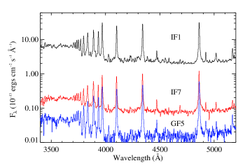
Figure 36: Flare-only gradual decay phase spectra from IF1 (black), IF7 (red), and GF5 (blue) on YZ CMi. These data have the same spectral resolution, revealing many features in common between the smallest and largest flares in the sample.

Three flares – IF1, IF7, and GF5 – are particularly interesting to compare because they occurred on the same star and the data were obtained at the same spectral resolution (1.83Å pixel^-1, using the 1.5″ slit). The gradual decay phase spectra of these three flares on YZ CMi are presented in Figure 36 (from the times given in Table 5). These comprised the smallest amplitude flare (GF5, blue), a medium-amplitude flare (IF7, red) and the largest amplitude flare (IF1, black) in the sample. At the times of these spectra, the $U$-band was emitting at 1.4, 2 and 25 times the quiescent level, respectively. The best-fit $T_{\mathrm{BB}}$ values are 7600 K for IF7 and 8300 K for IF1. GF5 has very low amounts of emission, but is fit nonetheless with $T_{\mathrm{BB}}$$\sim$4900 K.

Despite these differences, there are striking similarities across the NUV and blue-optical zones, including 1) small-scale features at the base of the Hydrogen lines; 2) the appearance of the prominent Helium i lines at $\lambda$4471 and $\lambda$4026, He ii at $\lambda$4686, Ca i at $\lambda$4227$+$Fe ii at $\lambda$4233, and Fe ii (or Mg ib) at $\lambda 4924+$$\lambda$5018$+$$\lambda$5169; 3) two plateaus in the underlying level of the pseudo-continuum (one from $\lambda$$=3780-3950$Å and one from $\lambda$$=3650-3760$Å); 4) Hydrogen lines resolved through H14 at $\lambda$3722Å (H15 at $\lambda$3712Å, H16 at $\lambda$3704Å, and He i at $\lambda$3704Å are blended); 5) similar small-scale features, which may be blended Fe and Ti lines in emission in addition to the Balmer continuum emission at these wavelengths (e.g., $\lambda\sim 3580$Å, 3680Å). These qualitative similarities and the scaling relationship given in Section 7.1 illustrate that the gradual emission is nearly identical, but “scaled up” in flares according to their amplitudes and energies. Clearly there are important similarities in the gradual decay phases of flares covering a large range of impulsive phase peak amplitudes and energies.

8 The Third Continuum Emission Component: A “Conundruum”

Finally, we bring attention to the continuum rise at $\lambda$$>4900$Å in Figure 36, representing excess “conundruum” flux above the best-fit blackbody that is present during the gradual decay phase of some flares (IF1, IF2, IF3, IF7, HF1, HF2, GF3, and GF5). The feature is also apparent in some peak spectra (MDSF2 of IF1, IF2, IF3, IF4, IF7, HF1, GF2; Figures 8 – 11). In the time resolved rise phase of IF3, this feature is detected starting at S#25, which is the first spectrum showing a hot ($T_{\mathrm{BB}}$$\sim$$10\,000$ K) blackbody component in this flare. We first present the observational signature and quantitative properties of the “conundruum” flux (hereafter, Conundruum) during IF3. Then, we present several possible explanations of this new continuum component.

8.1 The Conundruum Flux Budget and Relation to the Red Continuum

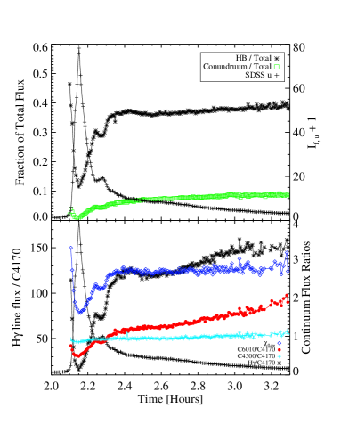
Figure 37: (Top) Time evolution of the Hydrogen Balmer (HB) flux ratio in the flare spectrum from $\lambda=3420-5200$Å compared to the time evolution of Conundruum flux ratio (green) for the IF3 event. The SDSS $u$-band light curve is shown in crosses (right axis). The Conundruum flux contribution increases as the gradual decay phase evolves. (Bottom) The evolution of the continuum flux ratios, C6010/C4170 (red), C4500/C4170 (turqouise), and C3615/C4170 ($=$$\chi_{\mathrm{flare}}$, blue) for IF3 shown on right axis. The smallest value of C4500/C4170 is 0.85 at peak (S#31). The line flux of H$\gamma$ (relative to C4170, asterisks, left axis) and the SDSS $u$-band light curve (black crosses) show much stronger reaction to the impulsive phase near flare peak.

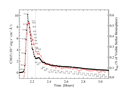
Figure 40: The evolution of derived and measured quantities for IF3: C3615 (black circles), $T_{\mathrm{BB}}$ ($\times 10^{3}$ K, numbered labels), and $X_{\mathrm{BB}}$ (right axis, red squares). The values of $T_{\mathrm{BB}}$ and $X_{\mathrm{BB}}$ are shown for every spectrum from S#25 – 44 and every four spectra after the end of the fast decay phase (indicated by a dotted line). For clarity, the values of $T_{\mathrm{BB}}$ are offset to the left of the respective C3615 points during the rise and peak, to the right of the respective C3615 points during the fast decay, and centered on the times of the respective C3615 points during the secondary flare ($t\sim 2.25$ hours) and the gradual decay phase. The vertical dashed line indicates the time of maximum C3615, and the vertical dotted line indicates the end of the fast decay phase.

The time-evolution of the Conundruum flux compared to other spectral features provide constraints on its origin. For IF3, we show the evolution of the ratio of HB to total $\lambda=3420-5200$Å flux in the top panel of Figure 37 (see Section 5.4). The evolution is nearly flat in the gradual decay phase. If we consider not just the ratio of HB to total flux, but instead the ratio of HB to blackbody flux (not shown), the ratio increases steeply in the gradual decay phase, similar to the trend in H$\gamma$ flux/C4170, which is shown in black asterisks in Figure 37 (bottom). Therefore, there must be an extra amount of flux in addition to the blackbody flux that contributes to the gradual phase emission to make the HB/total flux ratio in Figure 37 (top panel) approximately constant. From the excess flux (non-HB, non-blackbody) we also subtract Ca ii K, Ca ii H, the Helium i lines, and the Fe ii ($\lambda 4924+$$\lambda$5018$+$$\lambda$5169) triplet. The excess emission, which represents the Conundruum flux, is shown in Figure 37 (top panel) as green squares. The relative contribution steadily rises into the decay phase contributing a maximum of $\sim$9% of the total $\lambda=3420-5200$Å flare flux. We note that there is also a decreasing value of $T_{\mathrm{BB}}$ from $\sim$8000 K at the beginning of the gradual phase to less than 7000 K after $t\approx 2.7$ hours during this flare (see Figure 40, Section 10.2), which is probably due to the increasing contribution from the Conundruum at the redder end of the blackbody fit near $\lambda\sim 4800$Å, thereby affecting the blackbody fit. The Ca ii K line flux reaches its maximum at this time also (Figure 16).

In addition to becoming more apparent in the gradual decay phase, the Conundruum flux also has a larger relative contribution at redder wavelengths ($\lambda\sim 6000$Å). Here, we use a new continuum measure (C6010) in the red-optical zone (Table 3). In Figure 37 (bottom panel), several continuum fluxes are measured relative to C4170 for IF3 throughout its entire evolution: C6010, C4500, and C3615 (Table 3). In addition, we show the H$\gamma$/C4170 as a function of time (peak values for the sample were analyzed in Figure 13). Figure 37 (bottom panel) illustrates that, strikingly, C6010/C4170 has a similar time-evolution to $\chi_{\mathrm{flare}}$ and the H$\gamma$/C4170 ratio. The C4500/C4170 ratio, on the other hand, is relatively flat showing small variations that reflect the small changes in $T_{\mathrm{BB}}$ through the impulsive phase and into the gradual phase (see Section 10.2). The similar behavior seen between C6010/C4170 and H$\gamma$/C4170 suggests a time evolution of red-optical emission that more closely resembles the blue Hydrogen Balmer emission. In the decay phase, the C6010/C4170 ratio is more similar to the H$\gamma$/C4170 evolution than to the $\chi_{\mathrm{flare}}$ evolution. We conclude that the Conundruum has a relatively larger contribution at red wavelengths (C6010) and that its time-evolution is closer to the lower order Balmer lines (H$\gamma$, H$\beta$, and H$\alpha$) and Ca ii K than to BaC3615 (which contributes to the value of $\chi_{\mathrm{flare}}$).

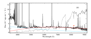
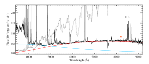
Figure 38: (Left) The $\lambda=3400-9200$Å flare-only spectrum during the gradual decay phase of IF1. The quiescent spectrum is shown as a dotted line. The blackbody fit to the blue optical is shown as the light blue line, the blackbody fit to the red shown as the red line. The red error bars is the height of the Paschen jump, $F_{\lambda=8200}-F_{\lambda=8300}$ offset vertically from the spectrum, predicted from the RHDF11 spectrum. (Right) The $\lambda=3400-9200$Å flare-only spectrum during the gradual decay phase of IF3 (with symbols shown as in top panel). In both panels, the Conundruum becomes apparent as the break in the spectrum where the blue and red lines cross at $\lambda\sim 5000$Å.

For several flares, we can directly measure the color temperature (spectral shape) of the Conundruum. In Figure 38 (left), we show for the first time a complete (gradual phase) flare SED from $\lambda=3400-9200$Å. This is an average of the spectra S#23 – 25 from IF1. The $T_{\mathrm{BB}}$ fit to the blue-optical zone is shown in blue and clearly does not account for all of the red continuum emission. The color temperature of the red optical zone (using windows RW1 – RW3, Table 4) for this flare ranges between $T_{\mathrm{BB}}$ $\sim 4500-5500$ K (fit shown in red). In Figure 38 (right), we show the complete SED during the decay phase of IF3 (time listed in Table 5). This flare also exhibits a red color, with a best fit blackbody temperature of $\sim$3700 K.

At the peak of IF3, the Conundruum is also apparent but with a smaller relative contribution to the total flux of C6010 compared to the gradual decay phase. In Figure 39, we show the extrapolation of a blackbody curve fit with $T_{\mathrm{BB}}$$=12\,100$ K to the blue-optical at the peak emission during IF3 (S#31) in order to illustrate the excess flux of C6010 unaccounted for by a simple isothermal Planck function that matches the blue-optical spectral zone. We tried various combinations of fitting Planck functions to the entire spectrum to account for the Conundruum. First, a single blackbody fit to both the blue and red optical zones reveals a temperature of $T_{\mathrm{BB}}$$\sim$$10\,200$ K; it fits the overall shape well, but misses the detailed shape of the blue-optical zone. If we fit a blackbody to the red optical zone only (using the continuum windows RW1 – RW3 in Table 4), we find a temperature of $T_{\mathrm{BB}}$$\sim$$7700$ K, but this fails to account for much of the blue-optical flux. Clearly, an isothermal fit cannot explain the full flare SED at peak.

Using a two-component blackbody to model the peak of IF3, we find that a combination of a $T$$\sim$$6000-6400$ K ($X_{\mathrm{BB}}$$\sim 1.5$%) blackbody and a superhot blackbody $T$$\sim$$10^{5}$ K – $3\times 10^{6}$ K ($X_{\mathrm{BB}}$$\sim 0.0042$%, $\sim$0.00012%, respectively) fit the $\lambda=4000-6800$Å flux distribution the best using the continuum windows BW1 – BW6 and RW1 – RW3 (Table 4). The optical signature of a very hot temperature ($T\gtrsim 10^{5}$ K) component can only be confirmed with bluer observations. Hawley & Fisher (1992) discuss that free-free emission from a superhot 1 MK source reproduces the optical ($UBVR$) colors of the Great Flare well but that it cannot account for the observed turnover of the broadband flux in the FUV and NUV.

It is possible that the large number of free parameters for two blackbodies allow an excellent, yet unphysical, fit to the IF3 peak spectrum. In particular, the two bluemost fitting windows (BW1, BW2; Table 3) may be contaminated from Hydrogen wing emission in such a large flare, therefore giving unrealistically large temperatures to fit the rise of the spectrum from $\lambda=4000-4150$Å. If we exclude the bluemost two continuum windows for the fit, we find that a combination of temperatures of $4700\pm 500$ K ($X_{\mathrm{BB}}$$=2.3$%) and $13\,700\pm 1000$ K ($X_{\mathrm{BB}}$$=0.17$%) and scaled by 0.98 fit the underlying $\lambda=4150-6800$Å continuum flux distribution the best (overplotted in red dashes in Figure 39). This fitting gives a hot blackbody consistent with a single temperature fit to BW1 – BW6 ($T_{\mathrm{BB}}$$\sim$$12\,100$ K; Table 7) and a single temperature fit using only BW3 – BW6 ($T_{\mathrm{BB}}$$\sim$$11\,000$ K; for further discussion on systematic temperature fitting errors, see Appendix F of Kowalski, 2012).

8.2 Possible Conundruum Interpretations

Possible explanations of the Conundruum are the following:

1. Calibration Artifact: We first considered whether the Conundruum was a calibration issue, as the DIS dichroic affects the flux calibration in the Johnson $V$-band range. The largest effect is near 5500Å (e.g., in flat-field lamp exposures). We took a conservative range and did not consider the flux between $\lambda$$=5200-5800$Å due to this issue.

2. Minor Species Emission Lines: It is well-known that spectra of QSO’s and Seyfert 1 galaxies have a forest of Fe ii lines between $\lambda$$=5000-5500$Å (Osterbrock, 1977; Puetter et al., 1981). There have been detections of strong Fe ii lines in stellar flares (Abdul-Aziz et al., 1995) and Fe i and Fe ii lines from solar flares (Severnyi et al., 1960; Johns-Krull et al., 1997) at these wavelengths. Other authors have aslo seen the presence of Fe lines in this range (Eason et al., 1992); many small scale features are visible in the high signal-to-noise spectra of IF1, and the Conundruum may be a blend of these lines.

3. Flux Redistribution from Minor Species Emission Lines: Due to the appearance of the iron forest at these wavelengths, line blanketing (Rutten, 2003) may cause the nearby continuum to increase, similar to flux redistribution generating a higher-than-expected effective temperature for the Sun (Böhm-Vitense, 1989). Higher spectral resolution data of flares from 4500 – 6000Å would help characterize bona-fide continuum regions. Line blanketing-induced continuum enhancements also need to be understood throughout the entire blue optical and NUV zones.

4. Non-Hydrogen Continua: There is a Helium ii continuum edge ($n=\infty$ to $n=5$) at $\lambda=$5694 Å. Helium ii continuum has been detected in solar flares in the EUV (Linsky et al., 1976; Milligan et al., 2012).

5. Continuum Fitting Artifact: By including the bluemost windows in the blackbody fitting (BW1, BW2), it could be a concern that we misfit the continua at longer wavelengths. These continuum windows have low-lying features within their narrow range. In extreme cases, the wings of H$\delta$ and H$\epsilon$ could contaminate the continuum windows. Appendix F of Kowalski (2012) tested whether removing BW1 and BW2 before fitting the blackbody function can explain the apparent Conundruum flux. In three of the four flares tested, various amounts of Conundruum remained after excluding these bluemost continuum windows.

6. Multithermal Flare Emission: The sum of all flare emission at any given time from a flare is very likely not isothermal; therefore, emission from regions (along all spatial directions in the atmosphere) with different temperatures would superpose to produce a spectrum that is inconsistent with a fit of a single blackbody over a large wavelength range. In Section 8.1, we were able to explain the blue-optical hot blackbody $+$ Conundruum contribution at the peak of IF3 using a double-blackbody fit (after minimizing the continuum fitting artifacts described in possibility #5).

7. Higher Order Hydrogen Continua: In Figure 2 of Kowalski et al. (2012), they accounted for the Conundruum through a superposition of model spectra using hot spot models and the RHDF11 model. The RHDF11 model ascribes the flux at redder wavelengths as due to a combination of Hydrogen Paschen continuum from the chromosphere and increased photospheric continuum that results from chromospheric backwarming. If the Conundruum has a large contribution from Paschen and possibly Brackett continua (Hydrogen recombination to $n=3$ and $n=4$, respectively); a subsequent transition to $n=2$ from either of these two levels would result in emission of an H$\alpha$ or H$\beta$ photon, respectively. This scenario could possibly explain the relation between the Conundruum and the lower order Balmer lines, which we discussed for H$\gamma$ in Figure 37 (Section 8.1). Higher order Hydrogen continua have been suggested to be a possible contribution to white-light radiation in the infrared (Tofflemire et al., 2012).

   In Section 9, we will discuss the interpretation of the Conundruum further and show that items #6 and #7 are the leading possibilities.

9 Comparison to Radiative-Hydrodynamic Stellar Flare Models

The contribution function from RHD models allows one to deduce the plasma conditions and detailed opacities that give rise to the predicted emission. For example, the BaC originates from a range of column masses where the electron density and chromospheric temperature structure are strongly coupled (Hawley & Fisher, 1992; Allred et al., 2006). Thus a simple optically thin, isothermal slab (e.g., Kunkel, 1970) does not provide an accurate estimate of the atmospheric parameters or the Balmer continuum originating from a real atmosphere. RHD models are required to give physically self-consistent values of $T$ and $n_{e}$ as a function of column mass in response to flare heating.

9.1 Comparison to the BaC and Conundruum Components

To model the flare Balmer continuum, we used the impulsive-phase RHD model spectrum at $t=15.9$ sec from the F11 simulation of Allred et al. (2006), hereafter A06, following Kowalski et al. (2010). We subtracted a linear extrapolation of the blue-optical zone in the model to estimate the amount of flux originating from the Balmer continuum. We refer to this model spectrum of the Balmer continuum as BaCF11 to distinguish from the published RHDF11 model. We repeated this calculation for the F10 model at $t=230$ sec from A06, giving an F10 Balmer continuum model spectrum BaCF10. These times (15.9 sec and 230 sec) correspond to the maximum amount of emission produced at $\lambda=4170$Å in the models. We calculated the spectral slopes, $m_{\mathrm{NUV}}$, of the BaCF11 and BaCF10 model spectra and give these values in Table 10 (columns 4 – 5) to compare to the observations in Table 7. The value of $m_{\mathrm{NUV}}\sim 5.1-5.5$ indicates that the model flux at 3420Å is $\sim$90% of the model flux at 3615Å. At the peak of the flares IF2, IF3, and IF9, the slope of the excess flux is blue ($m_{\mathrm{NUV}}<0$; column 11 of Table 7, Section 6.2) and is not consistent with the red slope of BaCF11 or BaCF10 ($m_{\mathrm{NUV}}>5$). Whereas the peak phases of the IF and HF events often show negative values of $m_{\mathrm{NUV}}$ (see columns 9 and 11 of Table 7), the GF events are more similar to the RHD predictions. This finding (determined from above) implies that our understanding of the impulsive phase Balmer continuum (and thus the flare chromosphere) is not complete with the current suite of RHD models. In the flare gradual decay phases, the IF and HF events tend to be more positive so the models may be more accurately portraying gradual decay phase (and GF) flare conditions.

To investigate the Balmer continuum in the gradual decay phase spectra in more detail, we added the BaCF11 model spectrum to the blackbody fit at $\lambda<3646$Å. The results are shown in red in Figures 30 – 34. We quantitatively compare the slopes of the observed Balmer continuum emission (after subtraction of the blackbody) to the slope of the BaCF11 ($\sim 5.1$) and BaCF10 ($\sim 5.5$) in column 5 of Table 10. In all of the gradual decay spectra, there is a relatively good match to the positive slopes (flux increasing towards redder wavelengths) of the model spectra, as we found for IF1 (Kowalski et al., 2010, see also Figure 30). The statistical fitting errors on the slopes (given in parentheses) are quite large, likely due to the difficulty in modeling the “true-continuum” underlying the forest of low-excitation metallic lines that are likely present in the NUV during the decay phase (Figure 36). There are also systematic errors due to flux calibration of $\sim$5 – 10% at these wavelengths (Appendix A of Kowalski (2012)); this uncertainty corresponds to about 2 – 4 in the units given in the table. The best matches to the BaCF11 model are obtained during IF9 and GF1, which have BaC slopes of 4.9$\pm 2.4$ and 5.9$\pm$1.3, respectively. We conclude that the observed BaC are reflecting flare chromospheric conditions from the models of A06, which apparently predict the gradual decay phase emission using (impulsive phase) RHD beam models having a non-thermal electron energy flux of $10^{10}-10^{11}$ ergs cm^-2 s^-1, a low energy cutoff of $E_{c}=37$ keV, and a power law distribution of nonthermal electrons with $\delta=3-4$. More accurately flux-calibrated spectra with higher spectral resolution (to resolve the faint metallic lines) extending further into the NUV will provide better constraints for the models.

The persistence of the BaC during late stages and the relatively good match to the shape of impulsive phase RHD model Balmer continuum, implies continued heating from accelerated particles during the gradual decay phase of these flares. Gyrosynchrotron microwave radiation has been detected far into the gradual phase of white-light flares on M dwarfs, suggesting that nonthermal particles are accelerated after the impulsive phase (van den Oord et al., 1996; Osten et al., 2005). Simultaneous, high cadence optical spectra, photometry, and radio data (e.g., from the EVLA) would better constrain the timing of gyrosynchrotron emitting particles and white-light radiation.

The impulsive phase RHDF11 model also accounts for the shape of the red optical Conundruum emission component rather well, with a best-fit blackbody temperature in the red of $T_{\mathrm{red}}\sim 4600$ K (RHDF10 shows about the same color in the red). This color temperature is similar to the color temperature of the total emission in the red-optical zone in the gradual decay phase of IF1 and to the color temperature of the cooler blackbody using a double blackbody fit in the peak phase of IF3. However, none of the RHD models (F10 or F11) show evidence for a color temperature of $\lesssim 4000$ K in the red part of the spectrum, as is needed to explain the red emission in the IF3 gradual decay phase. The RHDF11 spectrum predicts increased photospheric radiation from chromospheric UV backwarming and Paschen continuum from Hydrogen recombination in the flare chromosphere. The opacity description in the RADYN model does not include molecular features that are important in M dwarfs (e.g., TiO) and which would likely have a strong influence on the energy balance in the photosphere, and hence the backwarming physics. Modeling the backwarming is further complicated due to the large area over which it may originate (Fisher et al., 2012; Isobe et al., 2007). Obtaining separate models for the Paschen continuum and backwarming radiation is not currently possible with RADYN.

A reddening continuum shape during the gradual decay phase of IF0 in the $V$ and $R$-bands (covering $\lambda\sim 5000-7000$Å) was reported in HP91, who speculated about the presence of a Paschen continuum at these wavelengths. The best-fit blackbody temperature in the gradual decay phase to the $UV,UBVR$ photometry was $8400-8800$ K, similar to the lower temperatures we find in the gradual decay phase of the DIS sample using only the blue-optical continuum fitting. The mismatch to the blackbody continuum implied by these temperatures in Figure 11 of Hawley & Fisher (1992) (bottom two panels) is due to the addition of this red component. Excess flux in the $R$-band is also apparent in the moderate size flare on AD Leo described in Hawley et al. (2003). We speculate that the Conundruum rises into the red and accounts for the excess $R$-band flux observed in these studies.

Paschen continuum emission originating from typical temperatures ($6000$ – $8000$ K) of the flare chromosphere show a characteristic red color (Hawley & Fisher, 1992), and we consider the possibility that the red continuum emission (and hence Conundruum) is primarily due to Paschen continuum. From the RHDF11 spectrum, we estimated the height of the Paschen jump ($\lambda\sim 8204$Å) as $F_{\lambda=8200}-F_{\lambda=8300}$, which is 1/16.5 times the Balmer jump height ($F_{\lambda=3640}-F_{\lambda=3655}$). The predicted flux of the Paschen jump is shown in Figure 38 as red error bars indicating the height of the Paschen jump (using 1/16.5 times the flux of BaC3615). We do not find convincing evidence of a Paschen jump to indicate the presence of Paschen continuum emission, but the spectral region around the Paschen jump is contaminated by features from the Earth’s atmosphere and instrumental fringing which make the quiescent subtraction uncertain and the characterization of flare-only continuum difficult at these wavelengths. The Paschen jump has been (tentatively) detected in a solar flare (Neidig & Wiborg, 1984).

Using simple, isothermal, isodensity, optically thin, Hydrogen bf$+$ff slabs from Kunkel (1970) as a guide, we can explore the shapes of Paschen ($+$ Brackett) continua from $\lambda=3646-8205$Å. If we fit only to the red continuum, $\lambda=6000-6800$Å, $T_{e}=$ $12\,500-25\,000$ K (where $T_{e}$ is the electron temperature) is required to achieve a blackbody temperature of $T_{\mathrm{BB}}$$\sim$4500 – 5500 K (which corresponds to the color of the RHDF11 impulsive phase spectrum and the IF1 gradual phase red spectrum). If we consider the red gradual phase spectrum of IF3, which has a redder $T_{\mathrm{BB}}$ compared to IF1 ($T_{\mathrm{BB}}$$\sim$3500 – 4000 K), its shape is reproduced by an isothermal model with $T_{e}=7000-9500$ K. Clearly, a large range of electron temperatures ($7\,000$ – $25\,000$ K) can give rise to a relatively small range of red continuum colors ($T_{\mathrm{BB}}$$\sim$3500 – 5500 K). More advanced, multithermal, self-consistent, atmospheric modeling including photospheric opacity calculations is needed to make further progress in understanding this enigmatic continuum component.

9.2 Comparison to Peak Phase Blackbody Emission Component

The largest discrepancies between the current RHD models and the observations are the shape of the continuum emission in the blue-optical zone and the height of the Balmer jump. We measured the same observational parameters, $\chi_{\mathrm{flare}}$ and $T_{\mathrm{BB}}$, for the F10 and F11 continuum predictions from A06. The times analyzed are $t=230$ sec (F10) and $t=15.9$ sec (F11), respectively. We find that for the flare-only flux, $\chi_{\mathrm{flare,peak}}$$\approx$4.8 and $T_{\mathrm{BB}}$$\approx$5000 K for F10 and $\chi_{\mathrm{flare,peak}}$$\approx$8.2 and $T_{\mathrm{BB}}$$\approx$5300 K for F11 (given in Table 10). The values of $\chi_{\mathrm{flare}}$ are much higher than the observations ($\chi_{\mathrm{flare,peak}}$ between 1.5 – 4.5; Figure 13), indicating that the Balmer jump is too large. The color temperatures are far too low compared to the observations, which show a range at their peak times of $T_{\mathrm{BB}}$$\sim 9\,000-14\,000$ K (Section 6, 6.3). Using state-of-the-art observations and new diagnostics, we have revisited the long-outstanding problem that too much flare energy is deposited in the mid to upper chromosphere, where a large Balmer jump in emission is produced. In the RHD models, there is not enough energy deposited at high column mass (in the low chromosphere and photosphere) where a Balmer jump in absorption and/or blue-optical zone continuum with a shape similar to a blackbody having temperatures $T_{\mathrm{BB}}$$\sim$$9\,000-14\,000$ K can be generated (based on the phenomenological models of Cram & Woods, 1982; Houdebine, 1992; Kowalski et al., 2011a). Only when the impulsive phase “hot, blackbody” (white-light) emission is successfully reproduced by the models, can we begin to understand the detailed multithermal origin of the Balmer continuum, the Paschen continuum, the Conundruum, and the gradual phase 8000 K blackbody component; furthermore, we can then begin to understand how physical processes, such as flare heating, differ between GF and IF events and even between individual IF events. Thus, RHD models incorporating additional physics  –  such as higher energy electron beams and proton beams  –  are urgently needed.

10 Flare Filling Factors and Speeds

10.1 Continuum Emission Filling Factors

A physically significant quantity that can be derived from the spectra is the filling factor, $X$, which is the fraction of the area of the projected visible stellar disk that is emitting flare continuum emission. Values of $X$ for the white-light emission are often calculated in the literature (van den Oord et al., 1996; Hawley et al., 2003; Kowalski et al., 2010; Osten et al., 2010; Walkowicz et al., 2011; Davenport et al., 2012). Flare areas allow us to determine the degree to which individual stellar flares are “scaled-up” versions of one another (i.e., same spectral properties with larger area). Filling factors allow us to understand what type of heating distribution is responsible for the observed phenomena – i.e., using solar flare terminology, whether the flare heating is diffuse over a large area such as in extended ribbons or prominences, or whether the heating is focused into a small area such as in compact kernels. Finally, we find that filling factors are important for deriving the speeds of stellar flare development.

The area of a stellar flare is strongly dependent on the emission type used to model the spectrum. An important concern is that real stellar atmospheres do not produce featureless blackbody emission spectra. In Kowalski (2012), we investigated the corrections obtained using more realistic Castelli & Kurucz (2004) models of hot star atmospheres (summarized here in Appendix F), and we found that the corrected, inferred areal coverages (compared to those inferred from a Planck function) increase by a factor of $1.4-2.3$ for the peak temperatures of $T_{\mathrm{BB}}$$\sim$$9000-14\,000$ K in our sample. Moreover, the effective temperatures of the hot “blackbody” emission component can be estimated this way, giving $T_{\mathrm{eff}}$$\sim$$7700-9400$ K for this range of $T_{\mathrm{BB}}$ (for log $g=5$ atmospheres). The bolometric heating flux necessary to sustain the hot “blackbody” emission component is therefore $\approx 2-4\times 10^{11}$ ergs cm^-2 s^-1. Starting in Section 10.2, we correct $X_{\mathrm{BB}}$ using the algorithm in Appendix F.

We now discuss important systematic uncertainties when calculating filling factors of flare emission. First, there may be more than one source of continuum emission contributing to the total blue-optical (e.g., C4170) flare continuum emission at $\lambda>3646$Å at peak times during flares. For example, Conundruum flux likely extends into the blue (see Figure 38). The RHDF11 model predicts continuum flux at $\lambda>3646$Å, and this was used in the modeling of the continuum in Kowalski et al. (2012). Therefore, a single-component hot “blackbody” representation places only an upper limit on the areal coverage. We suspect that if the hot “blackbody” was the only source of blue-optical continuum, the absorption signatures seen in the Castelli & Kurucz (2004) models would be more prominent in flare spectra; even in giant flares, such as IF3 and IF4, the absorption phenomena only become measurable at peak emission when the hot “blackbody” has reached an areal coverage of $\sim$0.2% of the visible stellar hemisphere, corresponding to a physical area of $\sim$$3\times 10^{18}$ cm².

To calculate a filling factor for the (chromospheric) Balmer-continuum emitting region, we use the BaCF11 model from A06, as was presented previously for IF1 (Kowalski et al., 2010). Despite the discrepancy between the observed slopes and model slopes in the NUV spectral zone (Table 7 and 10), we use the RHD Balmer continuum flux to model the observed Balmer continuum as it is the best model we have currently available. A major source of uncertainty in the area of the Balmer continuum-emitting region is absorption predicted in the blackbody component (Castelli & Kurucz, 2004) at $\lambda<3646$Å: the Balmer continuum emission and absorption components are spatially unresolved in our stellar flare spectra. Interpreting the peak phase emission of IF2 using these hot star spectra, the measured amount of Balmer continuum flux (BaC3615) would be three times smaller than the intrinsic amount of Balmer continuum emission originating from the flare chromosphere if we also account for the absorption. In other words, a simple linear extrapolation from the blue-optical (as is used to calculate BaC3615 and therefore the filling factor of Balmer continuum emission) may vastly underpredict the true amount of chromospheric Balmer continuum emission. However, we note that preliminary modeling of “hot spots” in M dwarf atmospheres (Kowalski et al., 2011a) indicates that the amount of “missing” Balmer continuum flux is only $\sim$1.5 times the measured BaC3615.

Another important systematic uncertainty in the area of the Balmer continuum emitting region is our selection of the F11 model to represent the observed Balmer continuum flux. For example, using the Balmer continuum from the F10 RHD model of A06, we find that the inferred areal coverages of the BaC-emitting region would then be 8 times larger than inferred from the F11 model (Kowalski et al., 2010). The model BaC shape is not constrained from the observations due to the very small differences in the shape of the BaCF11 and BaCF10 between $\lambda=3420-3630$Å (Table 10). Given the discrepancy between NUV slopes observed at flare peak (for IF and HF events) and for these RHD models discussed earlier (Section 9), a method for discriminating between models would only be applicable during the gradual phase and peak phase of GF events. We are seeking to determine a method for constraining the appropriate model of the BaC.

Third, a more accurate modeling of the energy deposition by nonthermal electrons would take into account the pitch-angle distribution of electrons via the Fokker-Planck beam formulae (e.g., McTiernan & Petrosian, 1990). As the energy deposition is not as localized in the chromosphere, employing these formulae for a given beam flux would likely require the areas of the RHD Balmer continuum to be larger to account for the observed emission (Mauas & Gomez, 1997, A06).

Given these considerations, we calculate $X_{\mathrm{BB}}$, $X_{\mathrm{BaCF11}}$, and $X_{\mathrm{BaCF11}}$ / $X_{\mathrm{BB}}$ for all of the flares in the Flare Atlas. The values of $X_{\mathrm{BB}}$ (from fitting a blackbody, before applying the corrections in Appendix F) are given in Table 7 (column 7). At peak, the blackbody component exhibits an areal coverage on the order of $\sim$0.3% for the large amplitude flares, $\sim$0.03% for the medium amplitude flares, and $\sim$0.005% for the small amplitude flares, a range of $\sim$60x in area coverage in the DIS sample. We find that larger $U$-band emission at peak is due to a combination of both increasing blackbody and BaC areal coverage. The Balmer continuum emitting region is also compact, though larger than the blackbody component, originating from $\sim$0.05% to 1.7% of the visible stellar hemisphere. The ratio of the inferred surface area coverages ($X_{\mathrm{BaCF11}}$/$X_{\mathrm{BB}}$) is $1-26$ at peak, with the apparent amount of BaC originating from a larger area than the blackbody. However, the range of $3\leq$$X_{\mathrm{BaCF11}}$/$X_{\mathrm{BB}}$$\leq 15$ is found to represent most flares at peak emission; this range was also found during the decay phase of IF1 in Kowalski et al. (2010), as the flare went through successive impulsive and gradual phases of secondary flares. The largest luminosity flares have areal ratios of $\sim$$1-10$. The ratio of areal coverages, $X_{\mathrm{BaCF11}}$/$X_{\mathrm{BB}}$, after applying the corrections in Appendix F to the blackbody emission component, ranges between $2-8$ for twelve out of the seventeen flares with well-determined blue-optical temperatures. We predict that accounting for all of the aforementioned uncertainties in our area calculation would ultimately increase the Balmer continuum emitting area relative to blackbody emitting area. It would be instructive to recalculate the ratios of filling factors using more accurate RHD models of the Balmer continuum and blackbody emission components.

10.2 The Speed of an Expanding Flare Area

The IF3 event produced a rise phase lasting 2.7 minutes and a fast decay phase lasting 5 minutes, allowing a unique time-resolved study of the impulsive phase of a large-amplitude flare. Following the continuum analysis of Section 6.1, we fit a blackbody function to each spectrum from $\lambda=4000-4800$Å, and the filling factor, $X_{\mathrm{BB}}$, is corrected using the algorithm in Appendix F. The evolution of $T_{\mathrm{BB}}$ and $X_{\mathrm{BB}}$ is shown in Figure 40. The temperature evolution is as follows: almost immediately (S#25 – 26) in the fast rise phase, we measure a color temperature of $\sim$$10\,000$ K, which increases to $\sim$$11\,500$ K by S#27 when C3615 is 1/3 of the peak value. $T_{\mathrm{BB}}$ reaches a maximum value of $\sim$$12\,100$ K at the peak of C3615 at S#31. Whereas $T_{\mathrm{BB}}$ increases by $\sim$2000 K in the rise phase, $X_{\mathrm{BB}}$ experiences a large increase by a factor of 20 and stays elevated near its maximum value (possibly increasing very slightly) for three spectra after the peak. In subsequent spectra after the peak, the color temperature drops and then decreases monotonically at an average rate of $\sim$800 K min^-1 during the fast decay phase. At the end of the fast decay phase, the temperature reaches the characteristic gradual decay phase value of $\sim$8000 K. For equal C3615 flux levels during the fast rise and fast decay phases, the fast decay phase is more than 1000 K cooler, which implies that the area ($X_{\mathrm{BB}}$) must be greater during the fast decay phase. In other words, the fast rise is hotter and smaller than the fast decay. Mochnacki & Zirin (1980) observed similar impulsive phase trends for $X_{\mathrm{BB}}$ and $T_{\mathrm{BB}}$ using continuum data during several dMe flares from $\lambda=4200-6900$Å (e.g., see their Figure 3). The larger temperatures inferred from our data likely result from fitting a narrower spectral window ($\lambda=4000-4800$Å) to avoid contamination from the Conundruum component.

We now use the rate of areal increase ($X_{\mathrm{BB}}$) during the rise phase of IF3 to estimate the speed at which the flare area is changing, which can be used to constrain different scenarios of flare heating.

We use a simple flare areal model, whereby the white-light emitting region is circular with radius $r$, and the inferred filling factor, $X$, is changing at a rate $dX/dt$. The speed of the leading edge (perimeter) of the expanding circular flare area is given by

$$v(t)_{\mathrm{flare}}=\frac{dr(t)_{\mathrm{flare}}}{dt}=0.5\frac{dX(t)}{dt}\frac{1}{r(t)_{\mathrm{flare}}}R_{\mathrm{Star}}^{2}$$ (10)

where $r(t_{i})_{\mathrm{flare}}=(R_{\mathrm{Star}}^{2}X(t_{i}))^{1/2}$ and $\frac{dX_{i}}{dt}=(X_{i}-X_{i-1})/(t_{i}-t_{i-1})$ where $i$ is the spectrum number with midtime $t$. If instead we assume a more complex geometry having two expanding flare areas to represent the two footpoint structures observed during solar white-light flares (Hudson et al., 2006; Maurya & Ambastha, 2009), the inferred speeds decrease by a factor of two. Note, we use the filling factors $X_{\mathrm{BB}}$ adjusted using model hot star atmospheres of Castelli & Kurucz (2004) described in Appendix F. The uncertainties in the speed calculations are estimated to be $\sim$40%, primarily due to the systematic uncertainties in the temperatures (see Appendix F of Kowalski (2012)). An additional uncertainty results from possible projection effects (see footnote 22 in Section 6.1) such that a flare near the limb would show a smaller expansion velocity (by an amount proportional to ($cos$ $\theta$)^1/2, where $\theta$ is the foreshortening angle) compared to a flare at disk center.

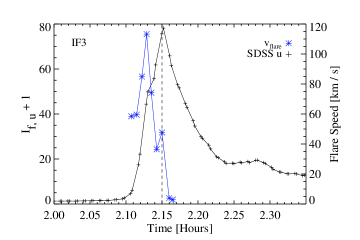
Figure 41: SDSS $u$ band enhancements (crosses, solid black line) and derived speed (asterisks, solid blue line) of the expanding flare perimeter during the rise phase of IF3. The dashed vertical line indicates maximum C3615 emission. See text for details.

We show the results for the speeds ($v_{\mathrm{flare}}$) during IF3 in Figure 41. According to this simple, circular flare model, the leading edge of the flare is moving at a high speed ($\sim 100$ km s^-1) during the rise phase and decreases to a small speed ($<10$ km s^-1) after the peak. The average speed during the flare rise is $\sim 50$ km s^-1, and the maximum speed ($\sim$110 km s^-1) is attained in the mid rise phase. The rise-phase speeds are supersonic for the photosphere and chromosphere of an M dwarf ($c_{s}\sim 5-10$ km s^-1) and we suggest several mechanisms below that could be responsible for the expansion rates observed. van den Oord et al. (1996) also considered the expansion speed of an erupting filament during a white-light flare on YZ CMi, and found $\sim$$100-500$ km s^-1, but they did not have spectra which are needed to determine the speed of the blackbody continuum component.

IF9 is another (IF) event in our sample where the blackbody has a rise and peak phase detection. Applying the same analysis, we find velocities of $\sim$130 km s^-1, $\sim$90 km s^-1, and $\sim$0 km s^-1 in the rise, peak, and fast decay phases, respectively. Although the uncertainties are again $\sim$40%, IF9 and IF3 show a similar pattern: fast speed in the mid rise, decreasing speed at peak, and very slow speed in the immediate post-peak phase.

We repeat these calculations for the rise phase of MDSF2 because it is a flare (albeit a secondary flare during IF1) with a simple, time-resolved rise phase. Only the average speed can be calculated for this flare. We find that during the rise phase, the area is expanding with an average speed of $\sim$8($\pm 3$) km s^-1, much smaller than during IF3. Although the flux calibration is less certain, IF4 is apparently a very quickly evolving flare exhibiting speeds of $\sim$65 – 150 km s^-1 through the rise and peak phases . We note in passing that both the “slowest” and “fastest” flares (MDSF2 and IF4, respectively) show signatures of Balmer wing depressions (Section 6.4) indicative of extreme heating scenarios, discussed in the next section. In Appendix G, we also consider the speeds during the HF1 and IF2 events.

10.3 The Meaning of Flare Speeds

There are several possible scenarios which could drive the expansion of a flare area, and we discuss the two most extreme here.

• Scenario 1 (Steady bombardment of a single region): $v_{\mathrm{flare}}\sim c_{s,\mathrm{chrom}}$, $dA_{\mathrm{beam}}/dt=0$

  For this scenario, we assume that the beam bombardment occurs at a fixed location and over a constant area ($dA_{\mathrm{beam}}/dt=0$). The sound speed is an important parameter for the expansion of a flare area occuring on the dynamical timescale in response to persistent beam heating from above (e.g., from the particles driven into the lower atmosphere during reconnection). As pressure equilibrium is achieved with the ambient atmosphere at the speed of sound, radiative and conductive heating lead to a temperature increase in the surrounding region. The rate at which the flare area expands is therefore related to the sound speed, and the rate at which the temperature increases is a combination of the rates from these heating processes which depend on the detailed physics and chemistry (e.g., specific heat) of the heated atmosphere. As the flare area expands, the average temperature may eventually drop because the beam heating (over constant area) can no longer sustain the temperatures against cooling from expansion. It is known from 1D RHD models that constant heating of a given region increases the column mass in the corona so as to inhibit further beam penetration (A06); future studies of this effect with (3D) RHD models would illustrate how relevant Scenario 1 may be during flares.

• Scenario 1b (Expanding bombardment of a single region): $v_{\mathrm{flare}}\sim v_{\mathrm{reconnection}}\sim c_{\mathrm{s,chrom}}$, $dA_{\mathrm{beam}}/dt>0$

  Scenario 1b is a variation on Scenario 1. The flare speed would also equal the sound speed if a sound wave can trigger magnetic reconnection and beam heating in nearby regions. Given that the sound wave disturbance persists for an extended duration, $dA_{\mathrm{beam}}/dt>0$.

• Scenario 2 (Sequential bombardment of multiple regions): $v_{\mathrm{flare}}\sim v_{\mathrm{reconnection}}>c_{\mathrm{s,chrom}}$, $dA_{\mathrm{beam}}/dt>0$

  A second scenario which may be important during the rise phase of impulsive flares, is transient, fast heating (sequential bombardment) of many small neighboring regions. In this scenario, the total area of all beams increase. This scenario allows for speeds larger than $c_{s}$ in the lower atmosphere without having to invoke shock heating. In fact, this scenario could occur at a speed which is driven by the speed of reconnection at heights (i.e., in the corona) above the site of flare heating. The emission we see at any given time is a superposition of all flare areas, and the increase of flare area during the rise phase is then related to the increasing number of these individually heated regions – not to the expansion of a single region. However, persistent heating and expansion could also be taking place simultaneously as each area that is heated by a beam expands according to the physics described in Scenario 1. An alternative explanation for Scenario 2 would be supersonic expansion of a flare area, resulting in heating contributions in neighboring regions from an expanding shock wave.

  Of the many important physical parameters that would inform this picture, we consider the depth of continuum formation and the decay timescale of the continuum to be essential information. Given the depth of continuum formation, we would know the relevant sound speeds and could test the relative roles of shock heating, conduction, radiative heating, and dynamical expansion. The timescale of continuum decay sets how long the beam needs to persist in individual flare areas in order to explain the observed amounts of emission.

We now discuss these scenarios given the derived speeds during IF3 and MDSF2. The average speed during MDSF2 is perhaps coincidentally, consistent with the speed (5 – 10 km s^-1) of the expanding disturbance from the initial $|\Delta U|\sim$6 mag at peak event (IF1) that was assumed to trigger MDSF2 in Kowalski et al. (2012). The slow speeds during the rise phase of MDSF2 are therefore consistent with Scenario 1b, giving a connection between the speed of a wave disturbance in the lower M dwarf atmosphere and the rate at which flare beam heating occurs at a new site. We speculate that the slower flare speed in MDSF2 led to more prolonged heating in a given area. In order to be consistent with the lack of Balmer line emission produced in MDSF2, it is also possible that the heating source was focused deep in the atmosphere (similar to the heights at which reconnection is thought to occur in order to produce Ellerman bombs, mentioned by Kowalski et al., 2012). These effects produced the higher color temperatures ($T_{\mathrm{BB}}$$\sim$$13\,000-15\,000$ K; Section 6.3 and Table 9) and more easily detectable absorption signatures.

Comparing the speeds for IF3 and MDSF2 signifies a physical connection between the flare speed and the type of blackbody spectrum (i.e., type of flare heating) observed. The average rise phase flare speed during IF3 is more than 5 times faster than the speed during MDSF2. IF3 produced large amounts of chromospheric (e.g., H$\gamma$, BaC3615) radiation, especially during the first half of the rise phase when the velocities were higher. If IF3 is described by Scenario 1, then the flare heating would have to be higher than the chromosphere ($c_{\mathrm{s,chrom}}\sim 5-10$ km s^-1) to be consistent with flare expansion occuring at large sound speeds. The rise and peak phases of IF3 are therefore most likely described by Scenario 2, implying that the areal increase would be related to the rate of individual areas being heated. Understanding the depth of formation of the IF3 continuum would allow us to place constraints on the heating of individual flare bursts so that the emission superposes correctly to form the observed light curve. At the beginning of the fast decay phase of IF3, the speeds decrease to $<$10 km s^-1, implying that Scenario 1 (or Scenario 1b) takes over after the peak. Unlike in the rise phase of MDSF2 (Scenario 1b) when the color temperatures are relatively high ($13\,000-15\,000$ K), the color temperatures in the fast decay phase of IF3 are decreasing and relatively lower ($\lesssim 11\,000$ K). Slow expansion is observed for a range of color temperatures, which may be related to the difference in heating mechanisms during the rise of MDSF2 and initial fast decay phase of IF3.

Additional, higher time resolution, data during the rise and fast decay phases of other types of flares would help us understand the relative importance of these scenarios and provide invaluable constraints on future 3D models that attempt to reproduce the formation of the hot blackbody continuum. In Section 11.4, we discuss the implications of flare speeds for the solar-stellar connection.

11 Discussion and Summary

In this study, we completed a homogeneous survey of twenty flares with simultaneous optical/NUV photometry and spectroscopy. We calculated and analyzed the following observational parameters: $t_{1/2}$ (the FWHM of the light curve; Section 3.1), the impulsiveness index $\mathcal{I}$ (peak $I_{f,U}$ divided by $t_{1/2}$; Section 3.1), $\chi_{\mathrm{flare,peak}}$ (C3615/C4170; Section 3.2), $\chi_{\mathrm{flare,decay}}$, BaC3615 (the Balmer continuum specific flux averaged between $\lambda=3600-3630$Å; Section 3.2), H$\gamma$/C4170 (Section 4.3.1), the fraction of $3420-5200$Å emission in the Hydrogen Balmer (HB) component (Section 5.4), $T_{\mathrm{BB}}$ (the color temperature of the continuum between $\lambda=4000-4800$Å; Section 3.2), $m_{\mathrm{NUV}}$ (the slope of the continuum between $\lambda=3420-3640$Å; Section 9), $X_{\mathrm{BB}}$ (the filling factor of the “blackbody” emission; Section 10), and $v_{\mathrm{flare}}$ (the speed of the expanding “blackbody”-emitting area; Section 10). Many of these parameters require an accurate flux calibration of the spectra, and we devised a new method for isolating the flare-only emission from background quiescent emission (Section 2.6, Appendix A).

We present a summary of the key observational results from this work in the first column of Table 11. In the second column, we suggest a possible physical interpretation of the observation. In the third column, we list the most critical parameter range for reproducing the impulsive phase hot ($\sim 10^{4}$ K), blackbody emission in future time-dependent modeling; this parameter range typically corresponds to the peak phase of the larger amplitude, IF events.

In the following subsections (Section 11.1  –  Section 11.7), we combine the main observational parameters to elaborate upon some of the physical interpretations in column 2 of Table 11. In particular, we discuss the origin of flare morphology, the interpretation of the hot, blackbody emission, and other astrophysical implications including the solar-stellar connection as revealed by the measured flare speeds.

11.1 Flare Morphology

How are the flare spectral properties related to the $U$-band light curve “morphology”? We began our study by separating the flares according to morphological characteristics from the broadband light curves, and we showed that the peak properties of the blue/NUV continuum are connected to the overall time-evolution of the light curve. We differentiate between impulsive and gradual flares according to a new value, the impulsiveness index, $\mathcal{I}$. Our designation is not to be confused with the impulsive and gradual phases of an individual flare: for example, a flare may be gradual if it has a low peak amplitude and/or large $t_{1/2}$ even though it may have distinct impulsive and gradual phases. The impulsiveness designation instead identifies the emission type (i.e., fast or slowly evolving emission) that contributes most to the overall evolution. The flares that had the largest value of $\mathcal{I}$ are generally the classical, impulsive flares (IF); the gradual flares (GF) are typically more complex featuring a slowly changing light curve near peak but also intermittent faster continuum variations. Some flares exhibited properties of both categories and are classified as “hybrid” flares (HF); these typically had several closely spaced (in time), fast yet resolved, continuum variations. Houdebine (2003) devised a similar classification scheme between “impulsive”, “gradual”, and “combined” flares. However, the Houdebine (2003) classification does not include white-light continuum emitting flares in the gradual flare category and our respective definitions for combined and hybrid flares differ: our definition includes the timescales of primarily the impulsive phase. Also, some of their combined flares would likely be included as impulsive flares according to our criteria.

Balmer continuum (BaC) in emission is ubiquitous during stellar flares, although it is present in varying amounts, contributing as little as $\sim$20% of the NUV flux (C3615) during IF events at peak and as much as $\sim$80% at peak of the GF events (Section 6.2, Figure 26), with the relative amount also decreasing as a function of flare peak amplitude. Though it dominates the relative flux in the GF events, the BaC is seen in large absolute amounts in some IF events (e.g., IF1, IF2, IF5, IF9). For the first time, we provide detailed light curves estimating the BaC emission from flare start to flare finish, and we find that it is generally similar to the Balmer lines, and evolves quickly, like the higher order Balmer transitions (as suggested in Doyle et al., 1988). The $t_{1/2}$ values of the Balmer continuum light curves for the well-measured flares were $\sim 5-20$ minutes, and future models should seek to reproduce this property.

We established a temporal relationship  –  the “time-decrement” (Section 5.2, Figure 20)  –  between six of the Balmer features for several flares. The time-decrement is a linear relationship between the wavelength of the Balmer transition and the $t_{1/2}$ value of the light curve for that transition. The time-decrement is similar for the classical flares IF3 and IF9, indicating a possible scaling relationship – similar heating parameters but over a larger area – between moderately large energy flares ($E_{U}\sim 10^{32}$ ergs) and high energy ($E_{U}\sim 10^{33}$ ergs) flares for the Hydrogen Balmer emitting region. The time-decrement for representative HF and GF events behaved differently than the IF events. For the HF event, the time-decrement behavior is probably affected by the superposition of two distinct flare impulsive phases. For the GF event, the flatness of the time-decrement is related to the larger ratio of $t_{1/2,\mathrm{C4170}}$ to the $t_{1/2}$ of the Balmer series; for the IF events, this ratio is normally very small.

To begin to understand the time-decrement, we look to Drake & Ulrich (1980), who related the larger energy difference to smaller collisional frequency between the upper level and any given lower level in the higher order lines compared to lower order lines. The time-decrement is therefore a result of each transition’s individual sensitivity to the decreasing densities in the flare chromosphere during the flare decay (see, e.g., Figure 7b and 10c of Drake & Ulrich (1980)) in addition to the different oscillator strengths in the formula for $C_{\mathrm{lu}}$ (Rutten, 2003). Due to the larger optical thickness, the lower order lines are less sensitive to the electron density of the flare chromosphere. The higher order lines and Balmer continuum emission are less optically thick and therefore have contributions from higher column mass (higher densities) where there are, generally, shorter cooling timescales, resulting in stronger sensitivity to $n_{e}$ and thus shorter $t_{1/2}$. In addition to density, the time decrement is likely dependent on several other important flare parameters in the decay phase: the change in chromospheric temperature structure, the sustained level of beam heating in the gradual phase, and the incident XEUV radiation field and overpressure from the superheated corona. Given all of these effects, which are changing as a function of atmospheric column mass and time during the flare, it is critically important to investigate the causes of the time-decrement with RHD models. Higher spectral resolution data of Balmer lines with high time cadence would help constrain electron densities (via the widths of the Balmer wings) in order to relate to the time-decrement behavior.

The continuum measured redward of the Balmer jump (C4170) is the fastest component in the blue/NUV and does not follow the time-decrement of the Hydrogen Balmer series. This continuum component contributes a large fraction of the emission throughout the NUV, blue-optical, and red-optical spectral zones, and we relate this to the “blackbody” emission continuum that has been detected in previous $\lambda>4000$Å spectral (Mochnacki & Zirin, 1980; Kahler et al., 1982) and $UBVR$ broadband color (Hawley & Fisher, 1992; Hawley et al., 2003; Zhilyaev et al., 2007) studies of flares. The $U$-band amplitude and time evolution are largely determined by the blackbody emission component although the $U$ band is also affected by the Balmer continuum, which adds to the flare emission at $\lambda<3646$Å. The BaC contributes relatively more flux in the HF and GF events and is the reason for their smaller amplitudes and more gradual time evolution as observed in the $U$ band. At peak, the percentages of C3615 (total NUV flux) due to BaC3615 are $\sim$20 – 44% (IF), 50 – 60% (HF), and 55 – 80% (GF; Section 6.2, Figure 26). The four flares with the smallest amount of Balmer continuum at peak relative to the total flux are the largest amplitude events: IF0, IF1, IF3, and IF4. We therefore conclude that the slower evolution of the GF events is due to a larger influence from the BaC, which is slower than the blackbody component (as characterized by $t_{1/2}$); conversely, the faster evolution of the IF events is due to the dominance of the blackbody emission component (most dominant in the largest amplitude flares), which evolves the quickest as diagnosed by C4170. The HF events are intermediate because of the approximately equal contributions of BaC and blackbody to the $U$ band at peak. Due to the largely different timescales among the spectral components, the relative amounts present at peak are therefore related to the overall light curve morphology. Clearly, a large sample was necessary for adequately understanding that not all stellar flares are identical, “scaled-up” versions of one another and that there are important spectral differences (presumably related to underlying flare heating mechanisms) to consider when modeling the gamut of flare behavior.

The IF events with the largest relative amount of Balmer continuum emission at peak are IF5 and IF6. These flares are also unusual for their IF designation with large $\chi_{\mathrm{flare,peak}}$($\sim$2.2$\pm(0.1-0.2)$), large H$\gamma$ to continuum ratios ($\sim$40 – 50), and a large fraction of Hydrogen Balmer (HB) flux ($\sim$40%) from $\lambda=3420-5200$Å. Coincidentally, these two flares both occurred on EV Lac. As illustrated by these two flares, the relative amount of one continuum component compared to the other is indeed variable even during the IF events. Nonetheless, the relative amount of Balmer continuum at peak generally determines the evolution of the flare as either impulsive (dominated by blackbody emission), gradual (dominated by Balmer continuum emission), or hybrid (both present, but generally more Balmer continuum emission). Also, the Balmer continuum does not always have a slow decay but is sometimes quite impulsive like the blackbody. This occurs typically with the hybrid flares (see the time-decrement relation for HF2; Figure 20), or for the impulsive flares with large $\chi_{\mathrm{flare,peak}}$.

Successful modeling of the exceptions within each classification scheme (e.g., IF5 and IF6 for the IF events; MDSF2 for the HF/GF events) undoubtedly will provide invaluable insight into the flare heating mechanism; this study awaits self-consistent modeling of the blackbody component which has not yet been attained.

11.2 The Balmer Jump

The main parameter we use to describe the blue/NUV continuum is $\chi_{\mathrm{flare}}$, the ratio of flux values to the blue (C3615) and red (C4170) of the Balmer jump. The IF events have small $\chi_{\mathrm{flare}}$ (and hence small Balmer jumps) at peak continuum emission whereas the gradual flares have larger Balmer jumps. We also measure the ratio of H$\gamma$ emission to the nearby continuum: H$\gamma$/C4170. We connected the size of the Balmer jump to the H$\gamma$/C4170, and find a suggestive linear trend such that flares with larger H$\gamma$/C4170 ratios have larger Balmer jumps (Section 4.3.1, Figure 14). Most of the IF events have strikingly similar $\chi_{\mathrm{flare,peak}}$ values of 1.6 – 1.8 over several orders of magnitude in flare peak amplitudes and energies. They generally also have H$\gamma$/C4170 ratios of 15 – 25 and only 11 – 17% of the emission in the Hydrogen Balmer (HB) component at peak. A narrow range of peak flare properties suggests a common impulsive heating mechanism among IF events. The $\chi_{\mathrm{flare}}$ and H$\gamma$/C4170 measures indicate the relative importance of each emission component – Hydrogen Balmer vs. blackbody emission – while also giving information about the flare morphology. $\chi_{\mathrm{flare}}$ is a measurement that can made without spectra, for example at very high time resolution and high signal-to-noise with the custom continuum filters used on the stellar instrument ULTRACAM (Dhillon et al., 2007; Kowalski et al., 2011b) and solar instrument ROSA (Jess et al., 2010).

For the IF events, the Balmer jumps increase by the beginning of the gradual decay phase ($\Delta$$\chi_{\mathrm{flare}}$$\sim$1) and also show 20 – 30% more blue and NUV emission in the Hydrogen Balmer (continuum and line) component compared to peak (Section 5.4, Figure 23). These trends indicate that the white-light heating/cooling mechanism in the impulsive and gradual phases of flares changes, as flares become more dominated by Hydrogen Balmer emission in the (fast and gradual) decay phases, which has been a phenomenon suggested by several works such as Moffett & Bopp (1976) and Abdul-Aziz et al. (1995).

The Balmer jump has not been detected in our low-resolution spectra (although we note that several instances in different flares show suggestive features near $\lambda\sim 3646$Å, especially in the gradual phase). It remains an open question what causes the large amount of apparent blending (which we have referred to as the “pseudo-continuum” or PseudoC) between $\lambda=3646-3914$Å, as the Balmer jump is not detected even in high spectral resolution, $R\sim 40\,000$ spectra (Schmitt et al., 2008; Fuhrmeister et al., 2008). We raise the question, what is the “Balmer continuum” that we observe in our low-resolution spectra? We suggest that the amount that we measure may be affected by the Stark broadening of higher order Balmer line wings and the continuum edge (Donati-Falchi et al., 1985). High spectral resolution, high time resolution data near $\lambda=3646$Å (while also covering some continuum regions at $\lambda>4000$Å in order to characterize the blackbody component) together with better modeling of the Stark broadening in the higher order Balmer lines (following the work of Donati-Falchi et al. (1985) for solar flares) are needed to understand the detailed pseudo-continuum properties from $\lambda=3646-3920$Å.

11.3 The Temperature of the Hot, Blackbody Component

The large percentage ($\sim$40 – 90%) of the wavelength-integrated blue$+$NUV (3420 – 5200Å) flux in the peak and gradual decay phases is emitted in continuum emission other than Hydrogen Balmer radiation for all flares (Table 8, Section 5.4). We attribute this continuum emission to a “blackbody” (or blackbody-like) source. We measured the slope of the blue continuum from $\lambda=4000-4800$Å and found it to be linearly decreasing with wavelength, thus allowing us to match it well to a blackbody with a moderately hot color temperature, $T_{\mathrm{BB}}$$\sim$$10\,000$ K (Section 6.1). The range of peak temperatures for the seventeen IF, HF, and GF events with well-measured slopes is between $T_{\mathrm{BB}}$$\sim$$9000-14\,000$ K (with systematic errors of about 1000 K; Figure 25). The secondary flare (MDSF2) during IF1 has the highest color temperature of $\geq 15\,000$ K at peak. The lowest temperature was measured as $T_{\mathrm{BB}}$$\sim$6700 K for the low-amplitude flare GF5. The flares for which we measured blackbody temperatures have a range of $\sim$2.5 orders of magnitude in flare peak specific luminosity in the $U$-band. Why such a narrow range of temperatures? We speculate that the origin and transient nature of the blackbody radiation may be due to a thermal regulation process, when a temperature threshold is reached in the deep atmosphere prior to runaway heating whereby material heats to higher temperatures and lower densities (i.e., “explosive evaporation”; see Fisher et al. (1985)). The observed Neupert relationship between Ca ii K and C4170 (the blackbody) may be indicative of an evaporative process occurring at high column mass (where C4170 is produced) if there is a connection between the formation of Ca ii K emission and the evaporated plasma through, e.g., X-ray (from $T>20$MK) radiative backwarming (Hawley & Fisher, 1992), condensations (Abbett & Hawley, 1999), or heat conduction channels (Canfield et al., 1984) from the corona.

We also explored interflare and intraflare $T_{\mathrm{BB}}$ variations. In Appendix G, we combined spectra from multiple peaks in a hybrid flare (HF1) to obtain a spectrum with the same total flux level of a very fast flare (IF2) and found bona-fide differences in the value of $T_{\mathrm{BB}}$, the fraction of HB to total flux, and the evolution of HB to total flux. Of the many parameters that could give rise to interflare $T_{\mathrm{BB}}$ variations, we suggested that the speed of the flare areal increase is an important parameter, which is summarized below. However, it is imperative that RHD models be used to model temperature differences between flares. With these state-of-the art spectral observations and new analysis techniques, we also attempted to constrain the intraflare variation of the blackbody continuum component. For two flares with time-resolved rise phases (MDSF2 and IF3; Table 9 and Figure 40), we found an apparent increase of $\sim$2000 K in the color temperature of the blackbody component during the rise phases.

The impulsive phase “blackbody” continuum component is not a featureless emission spectrum from $\lambda=3400-6500$Å. We detected an A-type star spectrum during the rise and peak phases of a secondary flare (MDSF2) that occurred during the Megaflare (IF1; K10). This finding gives important insight into the nature of the blackbody component: the absorption features and continuum shapes (i.e., $T_{\mathrm{BB}}$) encode information about the multithermal stratification of the flaring atmosphere at high densities. We hypothesize that the multithermal structure of the atmosphere is a byproduct of the thermal regulatory process, described above, such that the atmosphere responds in such a way that energy is most efficiently (and quickly) removed from the atmosphere through the continuum. We will explore this aspect of flare atmospheres in detail with future RHD models (Kowalski et al. 2013).

Absorption signatures were also detected in the wings of the Balmer lines during MDSF2 and IF4. Note that hot star-like absorption during flares also affects the Balmer flux and time decrements (Kowalski, 2012). Our analysis techniques can be applied to other flare observations to understand absorption phenomena in spectral data that lack broad wavelength coverage or robust flux calibration.

We extended the simple blackbody modeling to include the effects of flux redistribution and wavelength dependent opacities, as in a real stellar atmosphere, resulting in “Castelli-Kurucz” corrections which are described in detail in Kowalski (2012) and Appendix F. In summary, more realistic filling factors ($X_{\mathrm{BB}}$) of the “blackbody” emission component can be obtained, which are about a factor of 1.5 – 2.3 times larger, than those found using the Planck intensity to estimate areas. Also, effective temperatures can be estimated from the measured color temperatures of $T_{\mathrm{BB}}$ ($9000-14\,000$ K). The corresponding range of $T_{\mathrm{eff}}$ is $\sim$7700 – 9400 K (with the largest being $\sim$$10\,500$ K during the MDSF2 peak) indicating that at least $2\times 10^{11}$ ergs cm^-2 s^-1 is required for the heating flux to sustain the “blackbody” component. Detailed modeling of these “hot spots” in the M dwarf atmosphere would constrain the density and temperature stratification of the lower flaring atmosphere.

Most flares do not show obvious absorption features in the Balmer continuum or Balmer lines, likely due to the large amount of (chromospheric) Hydrogen Balmer flux in emission that generates an effective veiling of the photospheric absorption. The veiling leads to an anti-correlation in the apparent amount of Balmer continuum emission and the amount of blackbody-like continuum emission. As the absorption becomes greater  –  either through a larger filling factor (areal coverage) or because of higher blackbody temperature  –  the measured Balmer continuum emission estimated using a linear extrapolation from the blue-optical zone decreases. Again, accurate models (e.g., phenomenological “hot spot” models) would elucidate how much Balmer continuum emission is being missed.

An additional benefit of our large sample of flares and homogeneous analysis is evident. Not all flares have the same proportion of each emission component and therefore some flares reveal more about a given emission property than others. For example, MDSF2 exhibited a spectrum that had an unusually strong contribution from the “blackbody” component alone, thereby allowing unambiguous detection of the absorption features. The IF0 event from HP91 also had such a strong contribution from the “blackbody” component that the relative amount of Balmer continuum emission was among the lowest in the sample. In contrast, the IF1 decay phase showed an excessive amount of Balmer continuum emission, thereby allowing a thorough characterization of its flux and spectral shape. We predict that more observations will reveal additional, important variations in the flare continuum components that will contribute new constraints on flare models.

11.4 Flare Speeds and the Solar-Stellar Connection

We measured the speed at which the inferred “blackbody” flare area grows during the rise phase of IF3. We discussed ways in which the inferred flare areas are rather uncertain, and a more realistic determination was obtained by modeling the “blackbody” emission as a hot-star spectrum. During IF3, the speed is large in the early and mid-rise phase, with $v_{\mathrm{flare}}$ $\sim$100 km s^-1, decreasing to $\sim$50 km s^-1  at the peak and $<10$ km s^-1 in the post-maximum phase.

These speeds are strikingly similar to the speeds of the development of two-ribbon flares parallel and perpendicular to the magnetic neutral line in solar active regions. In particular, motions of white-light, hard X-ray, H$\alpha$  and Civ kernels are observed on the Sun (Kosovichev & Zharkova, 2001; Wang, 2009; Nishizuka et al., 2009; Krucker et al., 2011; Inglis & Dennis, 2012), and are observed to propagate at similar speeds of between $50-130$ km s^-1 during the development of two-ribbon structures parallel to the magnetic polarity inversion line (PIL) (Fletcher & Hudson, 2001; Schrijver et al., 2006). There is also slower motion perpendicular to the flare ribbons at the locations of the kernels, outward from the PIL with velocities of $\sim$15 km s^-1 (Fletcher et al., 2004; Keys et al., 2011) or as small as a few km s^-1 (Qiu et al., 2010), presumably the result of reconnection at progressively higher heights. Perhaps, the higher speeds in the rise phase are analogous to the formation of flare ribbons, and the smaller speed after flare maximum represents the perpendicular motions (e.g., “spreading moss”, Berger et al., 1999). This scenario has been deduced by UV/HXR observations to explain solar flare light curve morphology (Qiu et al., 2010).

The heating of new flare footpoints, resulting in increasing flare area, was a conclusion from the models of Hawley & Fisher (1992, 1994) to explain solar and stellar flare evolution. During solar flares, it is an open question what triggers particle acceleration (a possible source of flare heating) in neighboring flare regions (Inglis & Dennis, 2012). Possible scenarios are an unstable flux rope that erupts sequentially along a flare arcade (the “tether-cutting scenario” Moore et al., 2001) and magnetoacoustic slow waves that propagate away from the initial flare site (Nakariakov & Zimovets, 2011). Three-dimensional models of reconnection predict motions of the reconnection site, which undergo changes in velocity to slower speeds due to mass loading (Linton & Longcope, 2006).

The evolution of $v_{\mathrm{flare}}$ during IF3 (Figure 41) suggests that a similar (two-ribbon) flare development process involving sequentially heated footpoints occurs during solar and stellar flares, despite our likely over-simplification of the geometrical morphology of stellar flare regions (i.e., as an expanding circle). The quantity $v_{\mathrm{flare}}$ is therefore an exciting new measure that can be used to further address aspects of the solar-stellar connection. Broad wavelength coverage solar flare spectra (e.g., Neidig, 1983), which are not feasible with current standard instrumentation, would be invaluable for providing detailed insight into the spatially resolved continuum properties during ribbon and footpoint formation.

We also found a possible relation between the average speed during the rise phase and the temperature of the blackbody component at peak, with a very slow speed ($\sim$8 km s^-1) observed for hotter temperatures ($T_{\mathrm{BB}}$$\sim$$15\,000$ K) and prominent Balmer absorption features, e.g., in MDSF2. Perhaps the heating occurs by a process similar to solar Ellerman bombs on the Sun, where reconnection is thought to occur in the low chromosphere or photosphere. The connection to Ellerman bombs and their (possible) formation at high densities and low heights has implications for the heating properties of M dwarf flares that show Balmer absorption signatures. However, we do not exclude the possibility that the heating during the secondary flare MDSF2 (which is classified as a hybrid flare event; Figure 12) is connected to the Megaflare decay and may exhibit different heating properties than classical flares.

Determining the fundamental connection between speed and the type of white-light continuum emission will require further modeling work on the spatial development of flare regions. However, we began by comparing the speeds between flares and relating to two possible heating scenarios. We present two extreme scenarios: the expansion of a single hot spot in the lower atmosphere (Scenario 1, $v_{\mathrm{flare}}\sim c_{s,\mathrm{chrom}}$) and the formation of several hot spots (Scenario 2, $v_{\mathrm{flare}}>c_{s,\mathrm{chrom}}$). Insight into the detailed physics of these scenarios requires 3D modeling, but we can gain initial insight by comparing the speed of the flare to the speed of sound in the level of the atmosphere where the (blackbody) emission is formed. Higher speeds (50 – 130 km s^-1) are observed during the formation of a hot blackbody, $T_{\mathrm{BB}}$$\sim$$10\,000-14\,000$ K (Figure 25) and values of BaC3615/C3615 of 0.25 – 0.35 (Figure 26) for fast rise and peak phases of the classical flares IF9, IF3, and IF2 with moderate to large peak $U$-band amplitudes and energies. In the impulsive phase of these events, we find evidence of Scenario 2-type speeds during the rise and peak phases followed by Scenario 1-type speeds during the initial fast decay phase. A low speed ($\lesssim 10$ km s^-1) and high temperature were derived from the rise phase of MDSF2, whereas low speeds and relatively lower temperatures were derived in the initial fast decay phases of IF2, IF3, IF9, and HF1. Therefore, there is a range of heating that is observed at times of low flare speeds. The rise phase of MDSF2 is consistent with a variation on Scenario 1 (Scenario 1b), whereby the beam heating (and reconnection?) is triggered by a sound wave generated in the lower atmosphere by the initial flare peak of IF1.

11.5 The Conundruum Continuum Component

The white-light continuum persists well into the gradual decay phase of IF, HF, and GF events as the flare spectrum becomes increasingly dominated by Hydrogen Balmer (line and continuum) radiation. At the beginning of the gradual decay phase, the blackbody component exhibits a cooler temperature of $T_{\mathrm{BB}}$$\sim$8000 K. The change in color temperature from peak to gradual decay phase was first discovered by Mochnacki & Zirin (1980). We find that the evolution of C4170 (blackbody flux) begins to follow the Balmer continuum flux in the gradual decay phase. Another continuum component is detected redward of H$\beta$. This is observed as an increasing contribution of red flux during the flare gradual decay phase, and may be responsible for the redder colors seen in broadband photometry during the gradual decay phases of flares in the past (e.g., Kunkel, 1970; Hawley & Pettersen, 1991; Hawley et al., 2003). This “Conundruum” flux rises into the red spectral zone and has a color temperature of $\lesssim$5500 K during the peak and gradual decay phases. The colors in the red-optical are similar to those (albeit with large errors) reported during the gradual phase of a large flare on CN Leo (Fuhrmeister et al., 2008). This study found large temperatures ($\sim$20 000 – 30 000 K) in the red during the impulsive phase, whereas we find a peak phase color temperature of $T_{\mathrm{BB}}$$\sim$7700 K (using a single blackbody fit; Section 8). The Conundruum is present in some flares at peak also, but the hotter (blackbody) component dominates the white-light continuum shape at peak emission in the blue and, to a lesser extent, in the red. According to our analysis in Sections 6, Section 7, and Section 8, the red continuum ($\lambda\gtrsim 6000$Å) during dMe flares is a superposition of the hot, blackbody emission component and Conundruum emission component. Impulsive phase red emission (e.g., in the $R$ band) is largely due to the action of the hot blackbody component, and late phase gradual emission is largely due to the Conundruum.

The red spectral shapes are similar to RHD model predictions (Allred et al., 2006), from which we infer the origin of the Conundruum to be Paschen and Brackett recombination radiation from the flare chromosphere, and there may also be a contribution from H^- recombination radiation originating from a larger backwarmed area of the star (similar to the geometry in Fisher et al., 2012). We explored the Conundruum flux in detail for IF3, and suggest that it has a physical connection to the lower order (H$\gamma$, H$\beta$, and H$\alpha$) Balmer lines.

In summary, we find three continuum components that are important at different stages of the flare evolution: 1) Balmer continuum emission (most important in the mid rise phase and during the gradual gradual decay phase); 2) Hot “blackbody” emission (most important at the peak phase, but present with cooler temperatures in the fast decay and gradual decay phases); and 3) Conundruum emission (can be present in all stages, but most important in the late gradual decay phase).

11.6 One Flare Model to Rule Them All?

The emission at flare peak cannot be explained by simply scaling up small amplitude (e.g., in $U$ band) flares to get large amplitude flares, thereby implying important differences in heating mechanisms between IF, HF, and GF events. The emission components originate from different atmospheric parameters among the different types of flares, and even within a given flare type. We have shown several ways that IF3 and IF9 have scaled-up Balmer components (via the time-decrement; Section 5.2). However, the C4170 components appear to differ and do not follow a scaled up relation in their time evolution, suggesting that C4170 may be formed differently even among the IF events. We examined the scaling relationship between two flares in detail in Appendix G – HF1 and IF2 on YZ CMi – and concluded that one large peak phase is not a simple superposition of several smaller peak phases. Nonetheless, the $\mathrm{log}_{10}\mathcal{L}_{\mathrm{BaC3615}}$ vs. $\mathrm{log}_{10}\mathcal{L}_{\mathrm{C4170}}$ relation among the IF events with $\chi_{\mathrm{flare,peak}}$$<$ 2 and $T_{\mathrm{BB}}$$\sim$8000 K (IF2, IF3, IF7, IF8, and IF9) at the beginning of the gradual decay phase follow a linear relation, possibly indicating that these flares are scaled versions of one another after the fast decay of the C4170 (Section 7.1). Further evidence that gradual phase emission follows a scaling relation were deduced from a qualitative analysis (Figure 36) of the fine spectral features and continuum shapes spanning the gradual decay phases of IF1 (a large flare), IF7 (a medium amplitude flare), and GF5 (a small amplitude flare). One must independently consider the degree to which the Hydrogen Balmer (line and continuum) emitting region and blackbody continuum emitting regions are scaled between two flares and between individual flare phases. Furthermore, the production of the emission components is not mutually exclusive, as indicated by the short ($<1$ min) delay between the peaks of Hydrogen line emission and C3615 such as during IF3 and IF9 (Section 5.1). In fact, the sources of the emission components are intricately tied to one another via the flare heating mechanism and must be self-consistently accounted for in flare models that attempt to reproduce the evolution of these components and their variation during IF, HF, and GF events and during the impulsive and gradual phases of a given flare.

11.7 Connection to Other Astrophysical Phenomena

Transient astrophysical phenomena across the universe may be related to the underlying physics in the dMe flares, and we plan to explore these connections in a future paper. Here, we briefly note several interesting similarities to gamma ray bursts and accretion phenomena. Gamma-ray burst (GRB) light curves have been divided into two classes based on the duration of the hard X-ray light curves: Class I GRB’s with $2$ to several hundred second durations and Class II GRB’s with $<$ 2 second durations (Kouveliotou et al., 1993). Kouveliotou et al. (1993) further found that the Class II GRB’s exhibited harder spectral slopes in X-ray emission. Similarly, we found that impulsive flares have different optical timescales and spectral slopes (given by $\chi_{\mathrm{flare}}$) compared to gradual flares. Hurley et al. (2005) proposed that a Class II GRB originated from a magnetar flare (MF). The magnetar flares may be a subclass called soft gamma ray repeaters (SGRs) that occur relatively close to the Milky Way and account for only a few percent of the short/hard GRB’s (Palmer et al., 2005); the current leading model is the merging of two compact objects, one of which is a neutron star (Blinnikov et al., 1984; Nakar, 2007). Interestingly though, the impulsive phase of a MF has been fit well with a blackbody. In contrast to flare impulsive phase emission, the blackbody was found to have a much higher temperature $\sim$$2\times 10^{5}$ K. An impulsive phase in the light curve during times of prominent optically thick (blackbody or blackbody-like) emission is a similarity between dMe flares and magnetar flares and implies a common cooling (and heating?) process during the most luminous events in the solar neighborhood and the most luminous events in the universe.

A second astrophysical setting in which we find similarities to dMe flares is accretion, such as occurs in T Tauri stars and dwarf novae. The Balmer jump is a common diagnostic in T Tauri spectra (e.g., Valenti et al., 1993; Herczeg & Hillenbrand, 2008). In fact, some T Tauri spectra show small Balmer jump ratios that are rather similar to the $\chi_{\mathrm{flare}}$ values for flare spectra. Optical veiling from continua is often seen at $\lambda>4000$Å, which can inform our understanding of the “blackbody” continuum in flare spectra. Therefore, the physics of accretion models for T Tauri spectra can be used to inform our understanding of the white-light continuum. We also note that dwarf novae accretion events produce superposed Balmer line emission and Balmer line absorption features in their spectra, with most conspicuous absorption at times of maximum continuum emission that resembles an A or B type star (Hessman et al., 1984).

12 Future Work

Future RHD models should aim to reproduce the basic flare emission properties shown here: a hot blue-optical zone color temperature ($T_{\mathrm{BB}}$) and a small Balmer jump ($\chi_{\mathrm{flare}}$). The time-decrement will be important to constrain the time-evolution of the various flare types. Once the general $\lambda=3400-5200$Å properties are reproduced adequately, we should then aim to explain the PseudoC and lack of a Balmer discontinuity using a Hydrogen atom with many principal levels and a better treatment of Stark broadening (as in Johns-Krull et al., 1997). Understanding the red-optical continuum radiation will require an advanced treatment of photospheric molecular band chemistry and the effects of UV backwarming over large areas (Fisher et al., 2012).

We propose the following additional observations as future work:

• Our flare peak spectra (Figures 8 – 11) clearly indicate a rise toward bluer wavelengths into the NUV. Ultimately, models of blackbody emission must be tested in the NUV with spectral observations from $\lambda=2000-3400$Å. Unfortunately, there is a current lack of observational continuum measurements in this wavelength region during the impulsive phase of flares (of any morphological type) when the unexplained blackbody component is the brightest. NUV data at $\lambda<3400$Å are critical to constrain the detailed interflare and intraflare temperature variations in addition to the peak of the white-light (blackbody) emission.

• Observations of high-energy events with $|\Delta U|\sim 3$ magnitude (or greater) are important for establishing the occurrence and timing of small $\chi_{\mathrm{flare,peak}}$, Balmer continuum absorption, and line wing absorption during primary and secondary peaks.

• Moderate spectral resolution observations of $\lambda\sim 5000-5500$Å are needed to separate the contributions of Fe i and Fe ii emission lines from the Conundruum.

• High spectral resolution, high temporal resolution observations of $\lambda\sim 3500-4500$Å are needed to understand the blending of the higher order Balmer lines and the blending of the Balmer edge. Observations (at high time cadence) of H$\alpha$ would also be important for determining (directed and turbulent) mass motions during flares.

• High cadence observations of Ca ii K of very impulsive classical flares would help determine the degree to which the Neupert effect holds during flares. These observations would also constrain the evolution of flare area (via $v_{\mathrm{flare}}$) during this common, yet difficult to observe, flare type.

• High quality blue/optical/NUV spectral observations of the fast decay phase just after flare peak would provide insight into the transition from impulsive to decay phase emission. These observations are also important for understanding the behavior of $v_{\mathrm{flare}}$ (which is small) just after flare peak.

• More observations of flares with double-peaked impulsive phase broadband light curve morphology (like IF0, IF4, HF2, HF4) would constrain the complicated temporal relationship between the (Balmer and blackbody) continua and line emission. In these large, energetic, and relatively common events, the secondary flare may be the result of a triggering mechanism from the primary flare.

Figure 1: The peak (flare-only) spectrum from the flare ($t_{\mathrm{peak}}=2.6245$ hours) on 2010 Feb 14 on YZ CMi showing the windows of line flux integration for the H$\delta$, H$\gamma$, He i $\lambda 4471$, and H$\beta$ emission lines (dashed lines; see Table 3). The underlying continuum level was estimated using linear fits to the nearby regions indicated with dotted lines. These data were obtained with the 1.5″ slit.

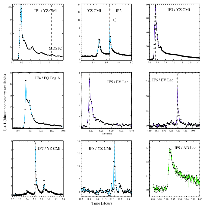
Figure 4: The impulsive flare photometry. The purple lines show photometry from the NMSU 1m (Johnson $U$), the light blue shows photometry from ARCSAT/Flarecam (SDSS $u$), and the green shows photometry from ARCSAT/Flarecam (SDSS $g$). The vertical dashed black lines indicate the time of maximum C3615. An arrow indicates the IF2 event. Time is the # of hours elapsed on the respective MJD from Table 6.

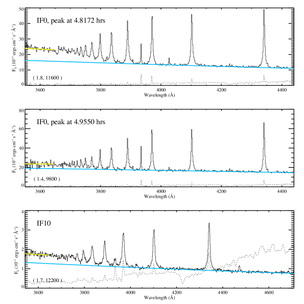
Figure 9: Top: The flare-only spectrum (S#36) at the first maximum continuum emission (C3615) of IF0. Middle: The flare-only spectrum (S#40) at the second maximum continuum emission (3615) of IF0. Bottom: The flare-only spectrum (S#31) at maximum continuum emission (C3615) of IF10. Note the long integration times in Figure 53 of Appendix B during IF10. The quiescent spectra are shown as dotted lines. The best-fit Planck function to the blue-optical region is shown in light blue. The yellow curve at $\lambda<3646$Å is the best-fit Planck function scaled to the C$3615$ flux. In parentheses, the $\chi_{\mathrm{flare,peak}}$ and the best-fit color temperature are given.

Figure 11: Same as in Figure 8.

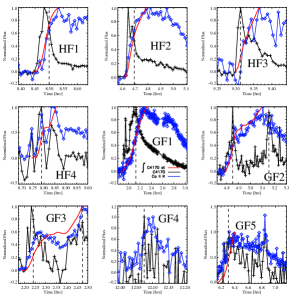
Figure 22: Same as for Figure 21 for the HF and GF events. The integral of C4170 is not shown for GF4, which has noisy continuum data. The Ca ii K flux follows the cumulative integral of C4170 particularly well (for times before the maximum of Ca ii K) for HF1, HF2, HF3, GF1, and GF2.

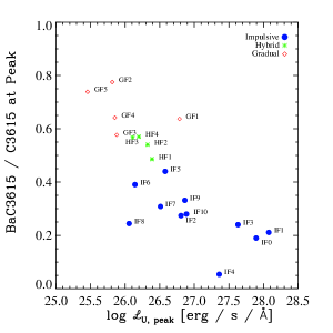
Figure 26: The fraction of the C3615 flux that is contained in the BaC3615 component. Note the decreased contribution from BaC3615 in larger amplitude flares and also in more impulsive flares.

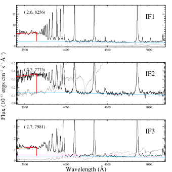
Figure 30: The flare-only gradual phase emission (black) compared to the quiescent emission (dotted line). Two-component model continuum fits are shown: the BaCF11 model in red, the best-fit blackbody in light blue. In parentheses, the $\chi_{\mathrm{flare,decay}}$ and $T_{\mathrm{BB}}$ are listed.

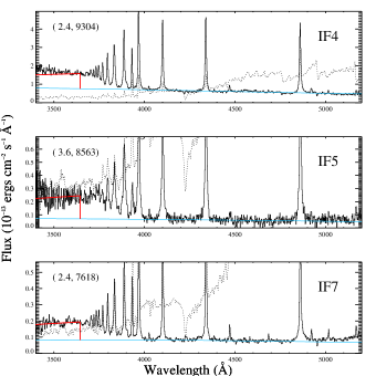
Figure 31: Same as for Figure 30.

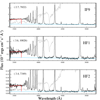
Figure 32: Same as for Figure 30.

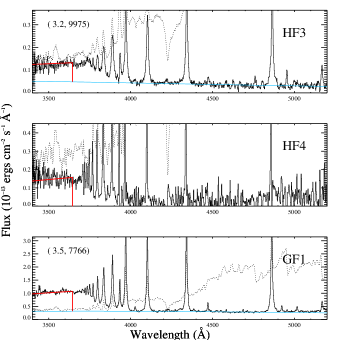
Figure 33: Same as for Figure 30. HF4 does not have well-determined values of $\chi_{\mathrm{flare,decay}}$ and $T_{\mathrm{BB}}$; only the BaCF11 model is plotted for this flare.

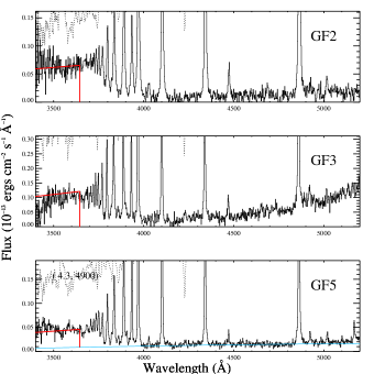
Figure 34: Same as for Figure 30. GF2 and GF3 do not have well-determined values of $\chi_{\mathrm{flare,decay}}$ and $T_{\mathrm{BB}}$; only the BaCF11 model is plotted for these flares.

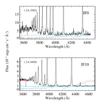
Figure 35: Same as for Figure 30. Note the different wavelength ranges. For IF10, we show spectrum S#32 (Table 5) which encompasses a secondary flare and the beginning of the gradual decay phase.

Figure 39: The peak flare-only spectrum of IF3 (S#31, black) from $\lambda=3400-9200$Å. The blackbody fit to the blue-optical zone (BW1 – BW6; Table 4) is shown in light blue. A fit using the sum of two blackbody curves (BW3 – BW6, RW1 – RW3) is shown as a red dashed line. The quiescent spectrum is shown as a dotted line.

Table 1: Target Star Basic Parameters

Star	Spectral Type	U	B	V	dist [pc]	R [RSun]	log $L_{U}$ [erg s-1]	$F_{U,q}$††
YZ CMi (Gl 285)	dM4.5e	13.77	12.80	11.19	5.97	0.30	28.6	1.35
EV Lac (Gl 873)	dM3.5e	12.96	11.86	10.28	5.05	0.36	28.8	2.85
AD Leo (Gl 388)	dM3e	11.91	10.85	9.32	4.89	0.43	29.2	7.49
EQ Peg A (Gl 896 A)	dM3.5e	13.18	12.12	10.41	6.34	0.36	28.9	2.33
GJ 1243	dM4e	$\sim$15.5†	14.47	12.83	12	0.36	$\sim$28.5†	0.27

Note. — Magnitudes are obtained from Reid & Hawley (2005); magnitudes for GJ 1243 are obtained from Reid et al. (2004). ^†The $U$-band magnitude and luminosity for GJ 1243 assumes that $U-B=1$. $L_{U}$ is the quiescent $U$-band luminosity and F_U,q is the quiescent $U$-band flux density. ^††Units of quiescent $U$-band flux density are 10^-14 erg s^-1 cm^-2 Å^-1.

Table 2: Observing Log

UT Date [MJD]	Time [Hrs]	Exp time [s] (# exp)	Slit [″] (Resolution [Å])	Photometry	Flares
YZ CMi
2009 Jan 16 (54847)	1.3	10 (157B, 163T, 0R)	1.5 (6, 13, 6.4)	1m ($U$)	IF1
2009 Jan 26 (54857)	6.183	20 – 45, 60, 300 (485B, 524T, 0R)	1.5 (5.7, 11, 6)	n/a	GF5
2010 Feb 14 (55241)	4.856	5, 10, 30, 45, 150 (332B, 424T, 83R)	1.5 (5.9, 12, 6.1)	1m ($U$)	IF7
2010 Dec 11 (55541)	5.028	18,30 (438B, 468T, 0R)	5 (17, 30, 12.5)	1m ($U$)	IF8
2010 Dec 13 (55543)	5.191	15, 18, 90 (574B, 606T, 0R)	5 (9.6, 30, 11.4)	1m ($U$)	HF3
2011 Feb 08 (55600)	5.580	8, 12, 15, 20 (610B, 703T, 0R)	5 (18, 31, 13)	1m ($U$), 0.5m ($g$)	IF2, HF1
2011 Feb 24 (55616)	3.988	7, 10, 12, 15 (437B, 462T, 0R)	5 (19, 32, 13.5)	0.5m ($ugri$)	IF3
2011 Mar 02 (55622)	3.921	20 (235B, 403T, 32R)	1.5 (7.3, 19, 7.4)	1m ($U$)	GF2
EV Lac
2009 Oct 10 (55114)	8.202	6, 15, 20, 30 (572B, 626T, 0R)	1.5 (5.5, 12, 5.5)	1m ($U$) 0.5m ($u$)	IF6, GF3
2010 Oct 11 (55480)	4.868	3, 5, 9, 10 (621B, 686T, 108R)	1.5 (7.3, 18, 6.5-7)	1m ($U$) 0.5m ($ugr$)	IF5, GF1
AD Leo
2010 Apr 03 (55289)	3.973	1, 2, 10 (431B, 581T, 145R)	1.5 (6.5, 15, 6-6.5)	0.5m ($g$)	IF9
2011 Feb 08 (55600)	2.856	2, 5 (409B, 446T, 109R)	5 (18, 31, 13)	0.5m ($u$)	GF4
EQ Peg A
2008 Oct 01 (54740)	9.215	20, 30, 40 (722B, 786T, 0R)	1.5 (6, 12, 6.1)	1m ($U$)	HF4, IF4
GJ 1243
2011 Oct 20 (55854)	2.830	45, 60 (135B, 159T, 0R)	5 (20, 31, 14)	n/a	HF2

Note. — Time is the total monitoring time for the night.

Table 3: Line and Continuum Windows

Line	Line Integration Window [Å]	Continuum Region [Å]
H$\alpha$	$6520-6610$	$6465-6484,6610-6665$
H$\beta$	$4828-4898$	$4813-4825$, $4895-4912$
H$\gamma$	$4310-4370$	$4260-4305$, $4375-4420$
H$\gamma$ (DAO)	$4321-4361$	$4260-4305$, $4375-4420$
H$\delta$	$4065-4135$	$4040-4064$, $4137-4167$
H$\delta$ (DAO)	$4084-4122$	$4040-4064$, $4137-4167$
H$\epsilon+$ Ca ii H	$3944-3997$	$3914-3923$, $4000-4017$
Ca ii K	$3923-3945$	$3914-3923$, $3946-3955$
He i $\lambda$4471 (1.5” slit)	$4464.6-4481$	$4380-4461$, $4488-4554$
He i $\lambda$4471 (5” slit)	$4460-4495$	$4380-4461$, $4488-4554$
Continuum Measure	Spectral Region [Å]
C$3615$	$3600-3630$
C$4170$	$4155-4185$
C$4500$	$4490-4520$
C$6010$	$5990-6030$

Table 4: Continuum Windows for Blackbody and Line Fitting

Name	Window [Å]	Comments
BW1	$4000-4015$	$n\lambda=8$
BW2	$4040-4057$	$n\lambda=9$
BW3	$4152-4210$	$n\lambda=31$, weighted by 0.97
BW4	$4495-4520$	$n\lambda=13$
BW5	$4562-4630$	$n\lambda=37$, line at 4584Å in IF1 decay
BW6	$4731-4800$	$n\lambda=37$, not used for fitting spectra from DAO
RW1	$5920-6120$	$n\lambda=71$
RW2	$6360-6470$	$n\lambda=39$
RW3	$6705-6845$	$n\lambda=50$

Note. — For the Great Flare (IF0), the higher spectral resolution data (and limited wavelength range) allowed fitting in BW1, BW2, BW3 and also in the windows, $3915-3922$Å  $4242-4287$Å, and $4400-4420$Å. $n\lambda$ is the number of wavelength points within each spectral window.

Table 5: Peak and Gradual Decay Phase Times

Flare ID	Peak Time [Hr] (S#)	Decay Time [Hr] (S#)
IF0	4.8172, 4.9550 (36, 40)	5.0825 (45)
IF1	2.1441 (113)	1.4576 (24)
IF2	8.6540 (542)	8.6747 (545)
IF3	2.1500 (31)	2.4512 (87)
IF4	10.4686 (665)	10.5690 (674)
IF5	6.1929 (516)	6.2205 (520)
IF6	4.7934 (261)	4.8300 (264)
IF7	2.6245 (19)	2.6785 (22)
IF8	11.6274 (390)	11.6506 (392)
IF9	3.9120 (121)	3.9508 (126)
IF10	4.9070 (31)	4.9828 (32), 5.1431 (34)
HF1	8.4909 (521)	8.5455 (527)
HF2	4.6452 (106)	4.7891 (114)
HF3	9.3138 (234)	9.3658 (241)
HF4	8.7889 (550)	8.8672 (557)
GF1	2.1265 (69)	2.3194 (101)
GF2	4.8504 (119)	4.9158 (127)
GF3	2.2317 (34)	2.3140 (43)
GF4	12.0746 (316)	12.1062 (323)
GF5	6.3106 (332 – 335)	6.3769 (336 – 345)

Note. — The time and spectrum number for the peak and gradual decay phases. The times are given as hours on the MJD of the event. Note that three spectra around the gradual decay time listed above are averaged for the gradual decay phase values in the figures and text (the spectra numbers and times before and after are not given in the table). The times for IF1 are given in “elapsed hours from flare start” as presented in Kowalski et al. (2010); see note on times in Section 3.2.

Table 6: Flare Summary Table (1): Key Photometry Properties

ID	Star	Date	$t_{peak}$***	$I_{f,U,\mathrm{peak}}+1$	ED [s]	$E_{U}$ [$10^{32}$ ergs]	$L_{U,peak}$ [$10^{29}$ ergs s-1]	$t_{1/2,U}$ [min]	$\mathcal{I}$
IF1	YZ CMi	2009 Jan 16	2.1441	208	$93\,690$	38	84.63	7.73	27.0
IF2	YZ CMi	2011 Feb 08	8.6540	12.2	690	6.2	4.50	0.48	23.3
IF3	YZ CMi	2011 Feb 24	2.1500	78.2	$45\,810$	18.5	29.98	3.82	20.2
IF4	EQ Peg A	2008 Oct 01	10.4686	21.4	4710	3.7	16.04	2.46	8.3
IF5	EV Lac	2010 Oct 11	6.1929	5.4	460	0.28	2.7	0.84	5.2
IF6	EV Lac	2009 Oct 10	4.7934	2.6	70	0.04	0.97	0.32	5
IF7	YZ CMi	2010 Feb 14	2.6245	6.4	810	0.33	2.19	1.18	4.6
IF8	YZ CMi	2010 Dec 11	11.6274	2.9	130	0.05	0.78	0.69	2.8
IF9	AD Leo	2010 Apr 03	3.9120	4.4	1300	2-4	5.11	1.47	2.3
HF1	YZ CMi	2011 Feb 08	8.4909	5.3	920	0.37	1.72	2.43	1.8
HF2	GJ 1243	2011 Oct 20	4.6452	5.4	500	0.86	1.29	4.19	0.93
HF3	YZ CMi	2010 Dec 13	9.3138	3.2	440	0.18	0.88	2.84	0.77
HF4	EQ Peg A	2008 Oct 01	8.7889	2.4	530	0.41	1.11	2.40	0.58
GF1	EV Lac	2010 Oct 11	2.1265	8.04	$10\,180$	6.20	4.29	13.02	0.54
GF2	YZ CMi	2011 Mar 02	4.8504	2.1	$2020$	0.81	0.43	3.68	0.3
GF3	EV Lac	2009 Oct 10	2.4744	1.87	570	0.35	0.38	2.88	0.3
GF4	AD Leo	2011 Feb 08	12.0746	1.32	80	0.12	0.48	2.13	0.15
GF5	YZ CMi	2009 Jan 26	6.3106	1.3-1.5	170	0.36	0.13	21	0.02
IF0	AD Leo	1985 April 12	4.8172, 4.9550	70.2 (43)	$50\,000$	79	88.06	3.53	19.6
IF10	EV Lac	2009 Oct 27	4.9069	45.4 (9)	8720	5.3	27.0	0.46	96

Table 7: Flare Summary Table (2): Key Continuum Observables and Derived Properties from Spectra

ID	C4170		$\chi_{\mathrm{flare,peak}}$	$\chi_{\mathrm{flare,decay}}$	peak		decay	NUV Slope ($m_{\mathrm{NUV}}$)†
	$I_{f,\mathrm{peak}}+1$	$t_{1/2}$ [min]			$T_{\mathrm{BB}}$[K]	$X_{\mathrm{BB}}$[%]	$T_{\mathrm{BB}}$[K]	Peak	Decay	Peak  –  BB	Decay  –  BB
IF1	11.5 (6)	8.8	1.51 (0.08)	2.65 (0.20)	$10\,800$	0.207	8300	0.1 (3.5)	1.5 (4.6)	14.9 (18.4)	4.1 (10.6)
IF2	4.1	0.6	1.74 (0.04)	2.67 (0.18)	$14\,100$	0.029	7800	-5.9 (0.0)	4.8 (1.2)	-6.4 (0.3)	8.3 (2.1)
IF3	20.1	3.6	1.61 (0.01)	2.66 (0.16)	$12\,100$	0.269	8000	-4.1 (0.1)	3.0 (8.1)	-4.2 (0.5)	4.7 (13.4)
IF4	7.3	1.1	1.27 (0.03)	2.28 (0.09)	$11\,200$	0.188	9300	-2.5 (0.1)	-6.9 (1.0)	34.5 (2.7)	-10.8 (1.3)
IF5	1.8	0.5	2.22 (0.11)	$\cdots$	$12\,000$	0.013	8600	-0.5 (0.3)	-0.3 (7.7)	5.0 (0.8)	6.8 (8.7)
IF6	1.2	0.9	2.19 (0.20)	$\cdots$	$\cdots$	$\cdots$	$\cdots$	-4.1 (1.4)	13.4 (9.1)	1.3 (4.5)	20.2 (15.2)
IF7	2.7	1.3	1.74 (0.05)	2.40 (0.19)	$11\,300$	0.030	7600	-1.9 (0.3)	6.3 (2.0)	2.8 (1.1)	9.1 (3.3)
IF8	2.9	1.0	1.62 (0.11)	$\cdots$	$13\,000$	0.006	$\cdots$	-3.3 (0.8)	40.7 (4.4)	3.9 (4.3)	44.3 (11.4)
IF9	1.8	1.0	1.77 (0.05)	2.74 (0.12)	$10\,300$	0.046	7800	-4.1 (0.0)	3.0 (1.4)	-7.0 (0.0)	4.9 (2.4)
HF1	1.8	2.4	2.33 (0.11)	3.60 (0.51)	$10\,700$	0.017	$10\,000$	-0.8 (0.1)	1.2 (8.9)	1.9 (0.2)	-4.7 (18.0)
HF2	1.9	3.5	2.58 (0.13)	3.40 (0.38)	$9500$	0.018	7300	-1.5 (1.7)	4.1 (3.7)	-1.2 (3.1)	7.3 (3.9)
HF3	1.4	1.4	2.83 (0.23)	3.20 (0.46)	$12\,000$	0.005	$10\,000$	-0.3 (0.2)	9.3 (3.7)	3.1 (0.5)	15.8 (3.5)
HF4	1.3	1.5	2.97 (0.24)	$\cdots$	$12\,000$	0.008	$\cdots$	-8.1 (0.3)	-8.3 (1.8)	-11.2 (0.6)	-9.2 (4.0)
GF1	1.9	15.0	3.17 (0.12)	3.46 (0.23)	$8900$	0.045	7800	2.1 (1.9)	4.6 (0.9)	3.9 (3.0)	5.9 (1.3)
GF2	1.15	0.7	4.32 (0.62)	$\cdots$	$\cdots$	$\cdots$	$\cdots$	1.9 (1.7)	13.8 (1.5)	1.4 (2.1)	8.1 (13.5)
GF3	1.87	2.2	2.99 (0.31)	$\cdots$	$12\,700$	0.003	$\cdots$	1.1 (2.6)	18.1 (12.4)	5.9 (4.8)	22.6 (9.5)
GF4	1.03	0.5	$\cdots$	$\cdots$	$\cdots$	$\cdots$	$\cdots$	5.1 (6.3)	19.0 (9.0)	11.1 (10.1)	17.2 (5.7)
GF5	1.04	0.9	4.28 (1.29)	4.26 (1.63)	6700	0.006	4900	11.0 (8.8)	-6.1 (4.0)	12.7 (10.3)	-29.9 (10.6)
IF0	8.7	11.7	1.8 (0.08)	2.4 (0.8)	$11\,600$	0.20	5600	-9.2 (3.2)	15.8 (9.8)	-19.8 (9.7)	9.7 (31.3)
			1.4 (0.12)		9800	0.44		8.1 (1.4)		52 (7)
IF10	1.3	$\cdots$	1.7 (0.12)	2.4 (0.2)	$12\,200$	0.020	6500	-11.8 (0.5)	0.0 (6.7)	-32.7 (2.3)	-5.0 (11.5)

Note. — Errors on $\chi_{\mathrm{flare}}$ values are given in parentheses. No values are given for those with large errors ($\sim$100%) on $\chi_{\mathrm{flare}}$. The units of $X_{\mathrm{BB}}$ are % of the visible stellar hemisphere; these values are derived from a Planck function and are not corrected using Appendix F.

Table 8: Hydrogen Balmer (HB) Properties

Flare ID	HB flux / Total flux		H$\delta$ / Total flux	H$\gamma$ / Total flux	H$\beta$ / Total flux	H$\alpha$ / Total flux	BaC3615 / C3615
	Peak	Decay	Peak	Peak	Peak	Peak	Peak	Decay
IF0	0.19, 0.12	0.44	0.017, 0.016	0.016, 0.018	$\cdots$	$\cdots$	0.34, 0.19	0.66
IF1	0.15	0.34	0.015	0.020	0.030	$\cdots$	0.21	0.59
IF2	0.13	0.32	0.009	0.009	0.007	0.005	0.27	0.58
IF3	0.11	0.37	0.008	0.008	0.009	0.008	0.24	0.59
IF4	0.03	0.29	0.003	0.003	0.005	$\cdots$	0.05	0.51
IF5	0.24	0.52	0.018	0.020	0.020	0.017	0.44	0.71
IF6	0.22	0.42	0.017	0.018	0.018	$\cdots$	0.39	0.83
IF7	0.15	0.32	0.011	0.012	0.013	0.010	0.31	0.57
IF8	0.12	$\cdots$	0.008	0.009	0.008	0.0005	0.24	$\cdots$
IF9	0.17	0.34	0.012	0.012	0.012	0.009	0.33	0.59
IF10	0.15	0.43	0.017	0.020	$\cdots$	$\cdots$	0.28	0.61
HF1	0.24	0.44	0.021	0.022	0.022	0.016	0.49	0.67
HF2	0.31	0.48	0.023	0.025	0.029	0.027	0.54	0.66
HF3	0.35	0.42	0.026	0.026	0.026	0.022	0.57	0.62
HF4	0.35	0.56	0.024	0.026	0.023	$\cdots$	0.57	0.89
GF1	0.38	0.43	0.030	0.031	0.032	0.027	0.64	0.69
GF2	0.48	0.64	0.035	0.039	0.046	0.054	0.78	1.0
GF3	0.35	0.50	0.030	0.030	0.030	$\cdots$	0.58	1.0
GF4	0.51	0.64	0.044	0.057	0.065	0.068	0.64	0.90
GF5	0.51	0.51	0.057	0.066	0.088	0.100	0.74	0.80

Note. — All values in the table are given as fractions, although they are often discussed as percentages in the text.

Table 9: Color temperature diagnostics of MDSF2

Spectrum #	Method 1	Method 2	Method 3
$t=0$ min; (S#101$+$S#102$+$S#103) / 3	$8\,400$	$\cdots$	$\cdots$
$t=2.7$ min; (S# 108$+$S#109) / 2	$9\,500$	$14\,900$	$13\,100$
$t=4.8$ min; S#113	$10\,800$	$17\,700$	$15\,000$

Note. — See Section 6.3 for a description of the methods.

Table 10: RHD Model Predictions

Model	$T_{\mathrm{BB}}$ [K]	$\chi_{\mathrm{flare,peak}}$	NUV Slope ($m_{\mathrm{NUV}}$)
			Peak	Peak  –  BB
F10 ($t=$ 230 s)	5000	4.8	7.3	5.5
F11 ($t=$ 15.9 s)	5300	8.2	5.4	5.1

Table 11: Summary Table

Observed Property	Physical Meaning	Modeling Goal
IF events have lower $\chi_{\mathrm{flare,peak}}$ ($\lesssim 2.2$) than HF or GF events ($\chi_{\mathrm{flare,peak}}$$\gtrsim 2.3$; Section 4.3.1); IF events have smaller BaC3615/C3615 values but over a relatively large range ($\sim$0.2 – 0.35; Figure 26).	There is less Balmer continuum radiation relative to the faster evolving $T\sim 10^{4}$ K blackbody radiation at peak in the flares with faster impulsive phases (IF events); slower impulsive phases (HF and GF events) have relatively larger amounts of Balmer emission which evolves slower than the hot, blackbody component.	$\chi_{\mathrm{flare,peak}}$ of 1.6 – 1.8; BaC3615/C3615 $\sim$0.25 at peak.
There is a large spread of H$\gamma$/C4170 at peak in the flares: $\sim$6 – 165, which is correlated with the type of flare (IF, HF, or GF) and with $\chi_{\mathrm{flare,peak}}$ (Section 4.3.1). The fraction of total flare flux at peak in an individual Balmer line is also correlated with the type of flare (Section 5.4).	$\chi_{\mathrm{flare}}$ is a diagnostic of the relative amount of Balmer line and continuum radiation compared to $T\sim 10^{4}$ K blackbody radiation. The Balmer lines follow the strength of the BaC radiation.	H$\gamma$ line flux/C4170 $\sim$15 – 25 at peak; H$\gamma$ line flux/total flare flux is $<1-2$% at peak.
The percentage of Hydrogen Balmer emission is anti-correlated with the $U$-band time-evolution (Section 5.4).	The blackbody continuum is relatively strongest in the impulsive phase but decays quickly. The Balmer emission, although bright at peak, decays less quickly than the blackbody. This explains the small Balmer jumps at peak, and larger Balmer jumps in the gradual decay phase.	At peak, the percentage of flare flux emitted in the Hydrogen Balmer emission from $\lambda=3420-5200$Å is $\sim$15%. In the gradual decay phase, it increases to $\sim$35%.
The timescale of the Balmer continuum is about twice as fast as the timescale of H$\gamma$ for single-peaked events ($t_{1/2,\mathrm{H}\gamma}=1.5-20$ minutes; Section 5.1).	The Balmer continuum emission originates from different atmospheric conditions with shorter cooling timescales than the H$\gamma$ line.	Reproduce BaC and Balmer line timescales.

Table 11: Summary Table, cont…

Observed Property	Physical Meaning	Modeling Goal
For the simple high-energy, impulsive flares (e.g., IF3 and IF9), the Balmer line emission and blackbody flux have peaks that occur within 1 minute of each another; flares with complex morphology (e.g., double-peaked impulsive phases) show larger separations in H$\gamma$ and blackbody peaks ($\Delta t\gtrsim 3$ minutes; Section 5.1).	Balmer line emission and the blackbody continuum are produced from a similar heating source during the rise phase; the late peaks of the Balmer lines may result from the superposition of two separate flares.	Tens of seconds ($<$ 1 minute) lag between blackbody peak (first) and H$\gamma$ peak (second) for simple, high energy events.
For the classical, IF events of relatively large energy (IF3, IF9), there is a linear time-decrement relation between the timescale and wavelength of the Balmer line transition (Section 5.2): higher order transitions (e.g., those in the PseudoC and the BaC) evolve faster.	Balmer line evolution is scaled by a multiplicative factor during simple, large flares.	Reproduce time-decrement Balmer line behavior.
The blackbody flux is the fastest evolving spectral component (Section 5.2). For the impulsive and hybrid events, $t_{1/2,\mathrm{C}4170}\sim$0.5 – 3.5 minutes (but can be much larger, $\sim$15 minutes, when it is similar to the evolution of the Hydrogen Balmer emission).	The heating threshold required to produce and sustain the blackbody continuum flux must be higher than the threshold for the Balmer line and continuum emission. The blackbody flux likely originates from higher densities with shorter cooling timescales than the Balmer line and continuum emission.	$t_{1/2,\mathrm{C}4170}$ 0.5 – 3.5 minutes.
The cumulative integral of the C4170 (blackbody continuum flux) is similar to the Ca ii K line flux until the time of maximum Ca ii K line flux (Section 5.3); delays and decreases in the Ca ii K flux are observed during the early impulsive phase of some flares.	The cumulative blackbody emission is tied to the evaporation of the lower atmosphere to coronal temperatures, producing enhanced XEUV radiation that heats a large area of neighboring chromospheric gas to the temperature of Ca ii K production.	Reproduce relation which holds well for IF6, IF7, IF9, HF1, HF2, GF1, and GF2.

Table 11: Summary Table, cont…

Observed Property	Physical Meaning	Modeling Goal
The peak emission in the blue-optical continuum ($\lambda=$4000 – 4800Å) is well-represented by a blackbody with temperatures between 9000 K and 14 000 K; applies over a range of peak amplitudes and morphological type (Section 6.1).	A large amount of heating occurs at high densities during dMe flares. This is a major shortcoming of solar-type non-thermal electron beam heating model predictions.	$T_{\mathrm{BB}}$$=10\,000-12\,000$ K (Section 6.1) and $F_{\mathrm{BB,Bol}}\sim 2-4\times 10^{11}$ergs cm-2 s-1 (Section 10.1).
Interflare variations of $T_{\mathrm{BB}}$ are significant (Appendix G, Section 6.3).	Temperature variations between peaks of different flares provide important constraints on the heating mechanism parameters	Full range of color temperatures at peak is 6700 K (GF5) to $15\,000$ K (MDSF2).
Other continua are needed to match the jump in flux from $\lambda=4000$Å to $\lambda<3600$Å: the pseudo-continuum of blended Hydrogen lines (PseudoC) and the Balmer continuum emission (BaC). At peak, the spectral shape of the BaC is similar to the hot blackbody shape (Section 6.2).	Some continuum emission in the NUV is due to Hydrogen recombination from the mid-to-upper flare chromosphere, but the total emission in the NUV is dominated by the shape of the hot blackbody.	At peak, the shape of the NUV flux ($\lambda<3630$Å) is similar to that of a blackbody with $T_{\mathrm{BB}}$$\sim$10,000 K.
Some flares show direct evidence of Hydrogen Balmer line and continuum absorption	The white-light continuum is formed from heating at high densities, within a non-uniform temperature stratification where Hydrogen Balmer and Paschen continuum opacities are large, as in a hot star like Vega.	C3615 $<$ C4170 for $T_{\mathrm{BB}}$$\sim$$13\,000$ – $15\,000$ K during slow, secondary flares with a $t_{1/2,\mathrm{C}4170}$ of nearly 9 minutes.

Table 11: Summary Table, cont…

Observed Property	Physical Meaning	Modeling Goal
Flux depressions in the Hydrogen Balmer wings are detected at $\sim\pm$10 – 30Å from line center at the peaks of some flares.	Extreme heating at peak produces Balmer absorption, which adds to the Balmer emission originating elsewhere in the atmosphere – at different heights or in distant regions on the surface.	Narrower line widths at maximum continuum compared to maximum line flux, with the wing flux depressions increasing from H$\beta$ to H$\delta$. Flares with very small Balmer jump ratios of $\chi_{\mathrm{flare,peak}}$$\sim$1.5 typically show the most conspicuous wing depressions; these flares are either large amplitude or have large values of $T_{\mathrm{BB}}$.
The gradual decay phase begins at the point when the flux in Hydrogen Balmer components (as a percentage of total flare flux) has increased by $\sim$20 – 30% compared to peak. Also, the Balmer jump ratio ($\chi_{\mathrm{flare}}$) becomes larger and the shape of the RHD model Balmer continuum spectrum is consistent with the observed BaC spectral slope (Section 7.1, 9).	Hydrogen recombination from the mid-to-upper flare chromosphere becomes more important as a radiative cooling process in the gradual decay phase; heating from a solar-type nonthermal electron beam is likely present in the gradual phase.	$T_{\mathrm{BB}}$ is 8000 K at the beginning of the gradual decay phase.
In the gradual decay phase, the specific luminosities of C4170 and BaC3615 increase in equal percentages between flares of different sizes (Section 7.1).	The production of Balmer and blackbody continua may be driven by a similar heating mechanism (solar-type nonthermal electrons) during the gradual decay phase; however, RHD models of solar-type nonthermal electron beams have not produced the $T_{\mathrm{BB}}$$\sim$8000 K component.	$\mathrm{log_{10}}\mathcal{L}_{\mathrm{BaC3615}}=-0.63(\pm 0.86)+1.03(\pm 0.03)\times\mathrm{log_{10}}\mathcal{L}_{\mathrm{C4170}}$ at the beginning of the gradual decay phase when $T_{\mathrm{BB}}$$\sim$8000 K.

Table 11: Summary Table, cont…

Observed Property	Physical Meaning	Modeling Goal
The best fit blackbody to the blue-optical zone does not account for all the continuum flux at redder wavelengths ($\lambda>4900$Å) during some flares. This “Conundruum” exhibits a color temperature in the red-optical zone of 3500 – 5500 K and is more important in the gradual decay phase than in the peak phase (Section 8).	RHD model spectra are consistent with this red continuum; higher order Hydrogen recombination (e.g., Paschen, Brackett) and possibly increased photospheric (H-) emission from UV backwarming are likely important contributions to the red flare flux in the gradual decay phase.	$T_{\mathrm{red}}<$$T_{\mathrm{BB}}$K in peak and decay phases, $T_{\mathrm{red}}\lesssim 5500$ K in gradual decay phase.
The rise phase of flares (e.g., MDSF2, IF3) features an increase in $T_{\mathrm{BB}}$$\sim$2000 K.	Areal increase is the dominant effect during the rise phase; a narrow range of interflare and intraflare temperature variation over a large range of $U$-band luminosities could be due to a temperature threshold that is reached during flare heating (see Section 11.3); heating threshold is reached relatively early in the flare.	$\Delta$$T_{\mathrm{BB}}$$\sim$2000 K during rise; $T_{\mathrm{BB}}$ independent of peak amplitude over $\sim$2 orders of magnitude.
The speed of the leading edge of a circular magnetic “footpoint” of $T_{\mathrm{BB}}$$\sim$$10^{4}$ K blackbody emitting area is calculated; during classical high energy IF events (IF3, IF9), large speeds of $\sim$100 km s-1 occur in the rise phase before decreasing to $\lesssim 10$ km s-1in the initial fast decay (Section 10.2).	Fast speeds are related to the rate at which individual, neighboring footpoints are heated (Scenario 2), whereas slow speeds indicate prolonged heating of a given footpoint or group of footpoints (Scenario 1); a similar two-ribbon development process (with parallel and perpendicular footpoint motions) on the Sun and on dMe stars (see Section 11.4).	Flare models with spatial evolution.
A slow speed ($\lesssim 10$km s-1) is observed in both the rise phase (MDSF2) and initial fast decay phase (IF2, IF3, IF9, HF1) and generates a range of color temperatures (Section 10.2).	There is a difference in heating mechanism between the slowly increasing area and temperature and slowly increasing area and quickly decreasing temperature.	Flare models with spatial evolution.

Appendix A Scaling Spectra Using Molecular Features

In this Appendix, we describe how we test the flux scaling algorithm’s accuracy (see Section 2.6) for recovering a pre-determined flare spectrum. To simulate a flare spectrum, we add a Planck function (for a given $T_{\mathrm{BB}}$ and $X_{\mathrm{BB}}$) to a quiescent spectrum which has been scaled to surface flux values using distance and $R_{\mathrm{star}}$ (Table 1). Three blackbody temperatures were used – $T_{\mathrm{BB}}$$=5000,10\,000,$ and $50\,000$ K – to sample a large range of possible flare spectral shapes. The flare surface flux was multiplied by a filling factor ($X_{\mathrm{BB}}$) to simulate the surface areal coverage. We then multiplied the resulting flare$+$quiescent spectrum by a constant factor, ranging from $0.7-1.3$ to simulate grey slit-loss or weather-induced flux variations. The resulting “observed” spectrum was then used as input to the scaling algorithm (see text) to determine if the artificial factor (0.7 – 1.3) applied initially was recovered.

The largest flares on dM stars have factors of $\sim$100 enhancements in the $U$-band flux ($I_{f,U}+1\sim 100$; we denote the flux enhancement by $I_{f}+1$; see Section 3.1). The filling factors necessary to produce this enhancement of $T_{BB}=5000,10\,000,$ and $50\,000$ K are 0.76, 0.016, and 0.0004, respectively. The smallest flares in our sample increase the $U$-band by a factor of $\sim$2. The filling factors necessary for this enhancement are 0.015, 0.0003, and 8$\times 10^{-6}$ for these temperatures, respectively. In addition to small and extremely large flares, we also model an intermediate to large amplitude flare, with $I_{f,U}+1\sim 18$.

The results of testing large and small flare areas with the algorithm are given in Table 16 (first and third rows for each of the three temperatures). The results indicate that for small flares, the algorithm determines precisely the correct predetermined multiple (0.7 – 1.3) that was applied to the total flare$+$quiescent spectrum. At the other extreme, for the largest possible flares, there are possibly large errors (overestimations) for the 5000 K flare, 10% errors for the $10\,000$ K flare, and 3% errors for the $50\,000$ K flare. However, none of the flares in our sample are this large ($I_{f,U,max}+1\sim$80 during IF3; and further it is unlikely that 76% of the surface is flaring with a temperature of 5000 K). This experiment supports the use of a large slit width (with hopefully good photometric conditions) when obtaining data on large flares. We note that the corrections for the data of the large flare on 24 Feb 2011 ($I_{f,u}+1$$\sim$80 at peak) are very minimal ($<2$%), consistent with robust flux measurements via the use of a wide slit and clear conditions. When the algorithm errs, it almost always overestimates the scale factor.

Finally, we determine the flare amplitude at which the algorithm begins to show large errors (rows 2, 5, and 8 of Table 16). Only for the 5000 K flare with an enhancement of $I_{f,u}\sim 40$ is there a significant ($>$5% error); for this amplitude flare, the hotter temperatures (rows 5 and 8 of Table 16) give scalings $\lesssim$3% different from the predetermined values.

In Figure 42, we show the result of scaling the spectral fluxes for a night (2010 April 03) with occasional cloud cover (and variable seeing). This figure shows the corrected and uncorrected fractional flux variations for synthetic $g$-band fluxes obtained from the spectra, compared to simultaneous $g$-band measurements using the ARCSAT 0.5-m SDSS $g$-band photometry.

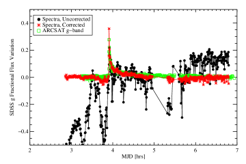
Figure 42: Variations due to occasional cloud cover are apparent in the raw (synthetic $g$-band) fluxes from the spectra obtained on 2010 April 03 (IF9) and shown as black circles. Our simple algorithm predicts corrections that adjust for these variations, allowing the flare to be characterized at wavelengths redder than the $U$-band where the fractional variations are smaller. The red asterisks are the adjusted $g$-band fluxes, which are a good match to the $g$-band photometry from ARCSAT (green, binned to the approximate exposure times of the spectra).

Table 16: Appendix Table: Scaling Spectra

$T_{\mathrm{BB}}$ [K]	$X_{\mathrm{BB}}$*	$I_{f,U}+1$	Algorithm Prediction**
5000	0.015	2	(0.70, 0.95, 1.05, 1.30)
5000	0.3	40	(0.73, 0.99, 1.1, 1.35)
5000	0.76	100	(0.82, 1.11, 1.23, 1.52)
$10\,000$	0.0003	2	(0.70, 0.95, 1.05, 1.30)
$10\,000$	0.0062	40	(0.71, 0.97, 1.08, 1.33)
$10\,000$	0.016	100	(0.75, 1.02, 1.14, 1.43)
$50\,000$	8$\times 10^{-6}$	2	(0.70, 0.95, 1.05, 1.30)
$50\,000$	0.00015	40	(0.70, 0.96, 1.06, 1.32)
$50\,000$	0.0004	100	(0.72, 0.93, 1.08, 1.33)

Note. — *The units of $X_{\mathrm{BB}}$ are fraction of the visible stellar hemisphere. **Scaling algorithm’s prediction for a set of scale factors corresponding to the following input, pre-determined scale factors: (0.70, 0.95, 1.05, 1.30).

Appendix B The Photometric Flare Atlas and Integration Times of the Spectra

In this Appendix, we show the photometry light curves and the integration windows of the simultaneous spectra (Figures 43 – 61). The grey shaded vertical bars show the integration time windows, and the S# is given on each grey bar. Note, these spectra correspond to the $n$B subcategory of spectra (see Section 2.2). The vertical red dashed line indicates the time at which the gradual phase emission is analyzed (Table 5). The three spectra nearest to this time are averaged for each flare to obtain the gradual phase spectra shown in Figures 30  –  34 for the flare sample. In all figures, times are given as elapsed number of minutes on the respective MJD from Table 2; for IF1 and MDSF2, the times are minutes elapsed from flare start (see note on times in Section 3.2).

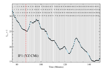
Figure 43: The $U$-band photometry (blue line, black circles) for IF1 and the spectral integration times given as shaded bars; the S#’s are indicated on each grey bar. The gradual phase spectra shown in Figures 30  –  34 are the result of averaging over the three spectra nearest to the vertical red line.

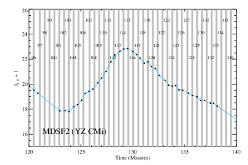
Figure 44: Same as Figure 43 but for MDSF2.

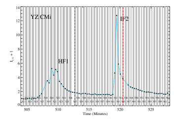
Figure 45: Same as Figure 43 but for IF2 and HF4.

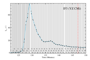
Figure 46: Same as Figure 43 but for IF3.

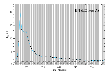
Figure 47: Same as Figure 43 but for IF4.

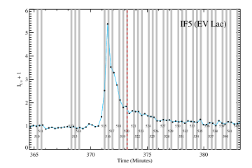
Figure 48: Same as Figure 43 but for IF5.

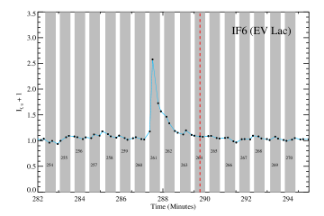
Figure 49: Same as Figure 43 but for IF6.

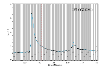
Figure 50: Same as Figure 43 but for IF7.

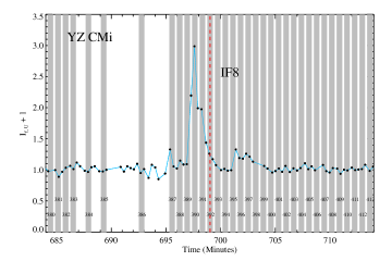
Figure 51: Same as Figure 43 but for IF8.

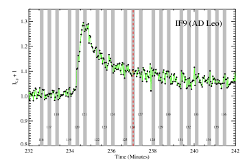
Figure 52: Same as Figure 43 but for IF9.

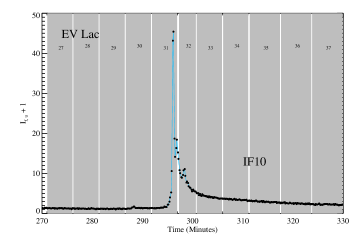
Figure 53: Same as Figure 43 but for IF10.

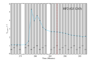
Figure 54: Same as Figure 43 but for HF2.

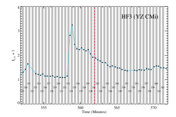
Figure 55: Same as Figure 43 but for HF3.

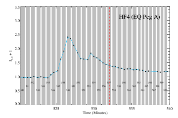
Figure 56: Same as Figure 43 but for HF4.

Figure 58: Same as Figure 43 but for GF2.

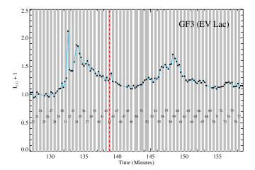
Figure 59: Same as Figure 43 but for GF3.

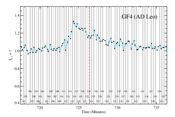
Figure 60: Same as Figure 43 but for GF4.

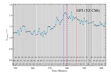
Figure 61: Same as Figure 43 but for GF5. The red lines indicate the boundaries of ten spectra used for the gradual decay phase spectrum. The purple vertical lines indicate the four spectra averaged for the peak spectrum.

Appendix C The Spectral Flare Atlas

Figures 62.1 – 62.21 show time sequences of the flare-only emission spectra for each flare in the Flare Atlas (Figure 62 shows a representative sequence of flare spectra during IF3; Figures 62.1 – 62.21 are available in the online version of the Journal). The top panels show the rise and peak phases, and the bottom panels show the fast and gradual decay phases. The color of each spectrum indicates the relative timing in the sequence (top panel: the order is black to blue to green to yellow to red; bottom panel: the order is red to yellow to green to blue to black; the number of colors depends on the number of spectra in the sequence), and the total duration of each time-sequence is roughly the same as for the light curves shown in Figures 4 – 7 (and Figures 43 – 44 for IF1 and MDSF2, respectively). The approximate time duration and range of S#’s (see Appendix B) are indicated in the top right of each panel. The grey shaded area indicates the wavelength range most affected by the DIS dichroic. Note, these spectra correspond to the $n$B subcategory (see Section 2.2) unless otherwise specified in the figure captions. The exposure times and dates of the observations are given in Table 2. The data (original unscaled flux and scaled flare-only flux) are available online through the VizieR service.

Fig. Set62. The Spectral Flare Atlas

Figure 62: (See published article for figure) A time-sequence of flare spectra (quiescent level subtracted) during the rise and peak phases (top panel, ordered by time from black to red) and fast decay and gradual decay phases (bottom panel, ordered by time from red to black) of IF3. For a complete description of the figure, see Appendix C. The emission line evolution is shown in Figure 16. A time sequence for each flare (Figures 62.1 – 62.21) is available in the online version of the Journal.

Appendix D Subtracted Flare Spectra

In Section 6.3, we found that newly formed flare emission (for MDSF2, the flux in spectrum S#113 with the background gradual phase emission, S#101 – 103, subtracted) resembles the spectrum of a hot star, like Vega. It is a concern, however, whether the background gradual phase emission continues to evolve (e.g., decrease) during the rise phase of the secondary flare, thereby resulting in an oversubtraction of the background flux. In this section, we show how our results change if we estimate the amount by which the previously decaying flare emission decreases over the course of the rise phase of MDSF2.

We estimate the decay phase timescale using a double exponential fit to the overall decay trend of the $U$ band in IF1 (see Figure 4). We then scale this fit by 90% to match the underlying level of the troughs in the decay phase. We predict that the $U$ band of the previously decaying emission would decrease by 5% from S#102 to S#113 (peak) and by 2.5% from S#102 to S#108 (mid-rise phase) if the secondary flare (MDSF2) were not present. Figure 63 shows the results of subtracting these adjusted background spectra. Qualitatively, our conclusions are the same. However, there are significant temperature differences for flare emission calculated using the unadjusted subtractions and the adjusted subtractions. For the unadjusted rise and peak phase spectra, $T_{\mathrm{BB}}$ is $14\,900$ K and $17\,700$ K, respectively. For the adjusted rise and peak phase spectra, $T_{\mathrm{BB}}$ is $13\,100$ and $15\,000$ K, respectively. Thus, accounting for the decay of background gradual phase emission from IF1 decreases the derived temperatures of MDSF2 by $\sim$1800 – 2700 K. Note, the detection of the Balmer continuum and lines in seen, and is robust result. The identification of “hot star” emission is therefore confirmed.

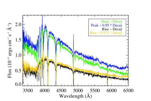
Figure 63: The flare-only spectra during MDSF2 rise (black) and peak (green), as shown previously in Figure 27. We adjust for an approximate amount by which the previously decaying emission evolves to the rise phase time (yellow) and peak time (blue).

Appendix E Possible Evidence for Wing Absorption at the peak of IF3

The flare IF3 has an impulsive phase with the largest continuum enhancement ($I_{f,u}+1\sim 78$) with spectral coverage in the DIS sample. The inferred areal coverage of the $T_{\mathrm{BB}}$$\sim$$12\,000$ K emission is large (Section 6.1, Table 7), and we search for evidence of wing depressions signifying the presence of hot star-like Hydrogen Balmer absorption (see Section 6.4). These wing depressions provide new constraints for RHD models of deep heating in flares and are found in IF3 only during the newly formed emission at peak.

In Figure 64, we show the SDSS $u$-band photometry during the rise and peak emission. The black circles are the photometry data, and the asterisks represent the derivative of the light curve. The derivative is useful for diagnosing changes in this light curve which has an irregular cadence. At $t=2.14$ hours ($\sim$80% of the maximum emission) the derivative has decreased, indicating the presence of a transient maximum in the photometry; we interpret this as evidence of the end of a fundamental “burst” of emission during the rise phase. The derivative then increases, signifying a new burst of emission leading to the peak. The red squares represent the photometry interpolated (using a spline function) and rebinned to a constant fifteen second spacing, illustrating the same effect as the derivative. In Figure 65 we show evidence of wing depressions at the time of the IF3 peak for the newly formed emission in the peak emission “burst”. We assume that this burst corresponds to a different flare region on the star (in Section 10.2, we show that the rise phase corresponds to increasing flare area, suggesting that this assumption is valid), allowing the rise burst spectrum (S#29) to be subtracted from the peak burst spectrum (S#31). The green profiles show the normalized total flare emission at S#29 (this corresponds to the rise phase when the continuum flux is at $\sim$80% of the maximum – before the second flare burst), the turquoise profiles show the normalized total flare emission at S#31 (at maximum continuum emission), and the black profiles show the difference (using the unnormalized spectra) of S#31 – S#29. The integration times of these spectra are indicated with green and turquoise shaded bars in Figure 64. The line emission formed during the second burst has narrower Hydrogen line profiles; the wings are depressed relative to the total flare emission. The apparent amount of wing depression increases from H$\beta$ to H$\gamma$ to H$\delta$, as observed in IF4 and IF1, signifying that the amount of Hydrogen line absorption increases for higher order Balmer lines as occurs in the spectra of hot stars.

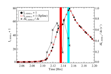
Figure 64: The SDSS $u$-band light curve of the rise phase of IF3 (left axis, black circles) and the first derivative of the light curve (right axis, asterisks). Sequential $u$-band observations have time-intervals of either 8 or 30 seconds. The vertical shaded bars correspond to the times of spectra used to obtain the line profiles during the first maximum (red) and peak (turquoise) phases of the flare shown in Figure 65. The $u$-band light curve is interpolated using a spline function and binned to 15 seconds (red squares, left axis) to show the smoothed evolution.

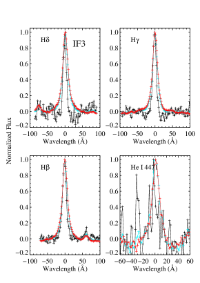
Figure 65: The H$\delta$, H$\gamma$, H$\beta$, and He I $\lambda$4471 of IF3 at $\sim$80% of the maximum continuum emission during the rise phase (S#29 normalized, red), at maximum continuum emission (S#31 normalized, turquoise) and the newly formed line emission at peak continuum (S#29 subtracted from S#31 then normalized; black). Before the normalization, the local continuum was subtracted with a linear fit. The times at which these spectra were taken are shown in Figure 64. The three Hydrogen lines all have narrower profiles in the newly formed peak flare emission, with H$\delta$ showing the largest effect.

Appendix F Corrections to $X_{\mathrm{BB}}$ using Hot Star Models

Correction factors for $X_{\mathrm{BB}}$ are determined from the ATLAS9 grid of LTE stellar atmospheres (Castelli & Kurucz, 2004) for a range of effective temperatures, $T_{\mathrm{eff}}=5000-16\,000$ K. Surface fluxes were calculated from the models with solar metallicity, $v_{\mathrm{turb}}=2$ km s^-1, mixing length parameter l/H$=1.25$, and log $g=5$. The color temperatures of all stellar models were measured using the continuum windows in Table 4. These windows were slightly adjusted to effectively match the model spectral shape from $\lambda=4000-4800$Å, resulting in a color temperature grid ranging from 3820 K to $23\,740$ K. The surface flux of each model spectrum was then compared to the surface flux of a blackbody (of the same color temperature) from $\lambda=4170-4210$Å and from $\lambda=4490-4530$Å. The ratio of the surface fluxes gave the correction factor to apply to the values of $X_{\mathrm{BB}}$ calculated from the blackbody fits.

Appendix G “Stacking Peaks”: Temperature differences in HF1 vs IF2

The flares HF1 and IF2 have respectively a higher ($2.33\pm 0.11$) and lower ($1.74\pm 0.04$) value of $\chi_{\mathrm{flare,peak}}$. They also occurred on the same star (YZ CMi), consecutively on the same night, at similar airmass, under similar weather conditions; thereby offering robust comparison of two flares with extremely different flare morphologies (multiple peak vs. single peak). During the impulsive phase of HF1, there were a series of peaks, and we ask the question whether adding the peaks together would produce the same spectrum as the main peak in IF2. If they match, then it is possible that the fast, large peak of IF2 is a result of smaller peaks (like those seen in HF1) that “stack” together very quickly below the time resolution of our data.

After adding HF1 S#518$-$S#521, the total flare-only emission in C$3615$ is $2\times 10^{-13}$ ergs s^-1 cm^-2 Å^-1, the same level as in the peak of IF2. Figure 66 shows the spectra (left panel) and the lightcurves (right panel). The spectra show noticeable differences in the blue-optical shape such that the stacked HF2 spectrum (black) has $T_{\mathrm{BB}}\sim 10\,700$ K and the peak IF2 spectrum (purple) has a steeper slope with $T_{\mathrm{BB}}\sim 14\,000$ K. There is also a difference in the relative amounts of H$\gamma$ to C4170 formed (ratios of 39 for HF1 and 17 for IF2) and the percentage of Hydrogen Balmer (HB) emission ($\sim$25% for HF1 and $\sim$15% for IF2). The evolution of the percentage of HB emission is shown in red asterisks in Figure 66 (right panel); in the gradual phase, a similar percentage is achieved ($\sim$40-45%), but the gradual phase value is attained relatively quickly in HF1 and more slowly in IF2.

This exercise has important implications for flare heating mechanisms. Larger peaks are not necessarily a straightforward “areal” sum of smaller peaks; instead, larger peaks can result from a larger temperature of the blackbody component produced from the flare. Flare heating during very impulsive events (IF2) may be more concentrated, temporally and spatially, in the atmosphere whereas several smaller peaks that are spread out in time (and space) may result from diffuse heating of several individual kernels over a larger area thereby producing a cooler blackbody in each kernel and relatively more HB emission.

We estimate the speed of areal increase (Section 10.2) to be $\sim$100 km s^-1 (rise/peak) and $\sim$15 km s^-1 (initial fast decay) for IF2 and $\sim$40 km s^-1 (fast rise and peak phase) and $\sim$5 km s^-1 (the fast decay) of of HF1. The inferred flare temperature (at peak) appears to be correlated with the speed for these two flares. In contrast, we found that the (rise phase) speed appears inversely correlated with the (rise and peak) temperature between MDSF2 and IF3. IF2 has a similar rise phase speed compared to IF3, for which we concluded that Scenario 2 type heating (Section 10.3) describes the development of the flare area. We speculate that it may be also important to consider the role of shock heating as a contribution to the larger temperature of IF2 (due to the inferred supersonic speed for the stellar chromosphere). Although the calculation of speed in HF1 may be affected by the presence of several distinct (temporally resolved, spatially unresolved) areas on the surface at a given time during the impulsive phase, there may be a difference in the flare mechanism or heating properties between a flare with slow speed but lower temperatures (HF1) and a flare with slow speed but higher temperatures (MDSF2).

Individually the area of each peak in HF1 is $<40-60$% the area of the blackbody in IF2 (Table 7), but the decay phase value of the percentage of HB emission is attained slowly in IF2; we speculate that this is reflecting the larger area of IF2 (hence, longer time to decrease in size assuming the beam heating turns off gradually). Ultimately, we hope to understand both the temperature and areal behavior using RHD models.

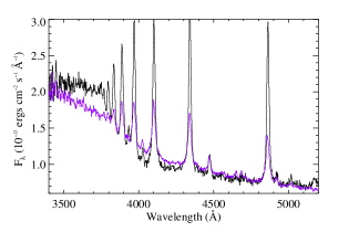
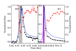
Figure 66: (Left) Comparison of stacked spectrum from the impulsive phase of HF1 (black) to the peak spectrum of IF2 (purple). (Right) The times considered are indicated in the right panel (shaded grey area and shaded purple area), which also shows the light curves for C4170 (black circles) and the $U$-band (blue line). The leftmost and rightmost axes are these quantities normalized to their peaks. The middle axis (referring to red asterisks) is the percentage of Hydrogen Balmer emission (Hydrogen Balmer flux / total 3420 – 5200Å flux; see Section 5.4) as a function of time.

References

- Abbett & Hawley (1999) Abbett, W. P., & Hawley, S. L. 1999, ApJ, 521, 906
- Abdul-Aziz et al. (1995) Abdul-Aziz, H., et al. 1995, A&AS, 114, 509
- Abranin et al. (1997) Abranin, E. P., et al. 1997, Ap&SS, 257, 131
- Allred et al. (2005) Allred, J. C., Hawley, S. L., Abbett, W. P., & Carlsson, M. 2005, ApJ, 630, 573
- Allred et al. (2006) Allred, J. C., Hawley, S. L., Abbett, W. P., & Carlsson, M. 2006, ApJ, 644, 484
- Berger et al. (1999) Berger, T. E., de Pontieu, B., Fletcher, L., Schrijver, C. J., Tarbell, T. D., & Title, A. M. 1999, Sol. Phys., 190, 409
- Bessell (1990) Bessell, M. S. 1990, A&AS, 83, 357
- Blinnikov et al. (1984) Blinnikov, S. I., Novikov, I. D., Perevodchikova, T. V., & Polnarev, A. G. 1984, Pis ma Astronomicheskii Zhurnal, 10, 422
- Bohlin (2007) Bohlin, R. C. 2007, in Astronomical Society of the Pacific Conference Series, Vol. 364, The Future of Photometric, Spectrophotometric and Polarimetric Standardization, ed. C. Sterken, 315
- Böhm-Vitense (1989) Böhm-Vitense, E. 1989, Introduction to stellar astrophysics. Vol. 2. Stellar atmospheres.
- Bopp & Moffett (1973) Bopp, B. W., & Moffett, T. J. 1973, ApJ, 185, 239
- Canfield et al. (1984) Canfield, R. C., Gunkler, T. A., & Ricchiazzi, P. J. 1984, ApJ, 282, 296
- Carlsson (1998) Carlsson, M. 1998, in Lecture Notes in Physics, Berlin Springer Verlag, Vol. 507, Space Solar Physics: Theoretical and Observational Issues in the Context of the SOHO Mission, ed. J. C. Vial, K. Bocchialini, & P. Boumier, 163
- Carlsson & Stein (1994) Carlsson, M., & Stein, R. F. 1994, in Chromospheric Dynamics, ed. Carlsson, M. (Oslo: University), 47
- Carlsson & Stein (1995) Carlsson, M., & Stein, R. F. 1995, ApJ, 440, L29
- Carlsson & Stein (1997) Carlsson, M., & Stein, R. F. 1997, ApJ, 481, 500
- Castelli & Kurucz (2004) Castelli, F., & Kurucz, R. L. 2004, ArXiv Astrophysics e-prints
- Christian et al. (2003) Christian, D. J., Mathioudakis, M., Jevremović, D., Dupuis, J., Vennes, S., & Kawka, A. 2003, ApJ, 593, L105
- Covey et al. (2008) Covey, K. R., et al. 2008, AJ, 136, 1778
- Cram & Woods (1982) Cram, L. E., & Woods, D. T. 1982, ApJ, 257, 269
- Crespo-Chacón et al. (2006) Crespo-Chacón, I., Montes, D., García-Alvarez, D., Fernández-Figueroa, M. J., López-Santiago, J., & Foing, B. H. 2006, A&A, 452, 987
- Cully et al. (1994) Cully, S. L., Fisher, G. H., Abbott, M. J., & Siegmund, O. H. W. 1994, ApJ, 435, 449
- Dal & Evren (2010) Dal, H. A., & Evren, S. 2010, AJ, 140, 483
- Davenport et al. (2012) Davenport, J. R. A., Becker, A. C., Kowalski, A. F., Hawley, S. L., Schmidt, S. J., Hilton, E. J., Sesar, B., & Cutri, R. 2012, ApJ, 748, 58
- de Jager et al. (1989) de Jager, C., et al. 1989, A&A, 211, 157
- Dennis & Zarro (1993) Dennis, B. R., & Zarro, D. M. 1993, Sol. Phys., 146, 177
- Dhillon et al. (2007) Dhillon, V. S., et al. 2007, MNRAS, 378, 825
- Donati-Falchi et al. (1985) Donati-Falchi, A., Falciani, R., & Smaldone, L. A. 1985, A&A, 152, 165
- Doyle et al. (1988) Doyle, J. G., Butler, C. J., Bryne, P. B., & van den Oord, G. H. J. 1988, A&A, 193, 229
- Drake & Ulrich (1980) Drake, S. A., & Ulrich, R. K. 1980, ApJS, 42, 351
- Eason et al. (1992) Eason, E. L. E., Giampapa, M. S., Radick, R. R., Worden, S. P., & Hege, E. K. 1992, AJ, 104, 1161
- Emslie (1978) Emslie, A. G. 1978, ApJ, 224, 241
- Filippenko (1982) Filippenko, A. V. 1982, PASP, 94, 715
- Fisher et al. (2012) Fisher, G. H., Bercik, D. J., Welsch, B. T., & Hudson, H. S. 2012, Sol. Phys., 277, 59
- Fisher et al. (1985) Fisher, G. H., Canfield, R. C., & McClymont, A. N. 1985, ApJ, 289, 425
- Fletcher & Hudson (2001) Fletcher, L., & Hudson, H. 2001, Sol. Phys., 204, 69
- Fletcher et al. (2004) Fletcher, L., Pollock, J. A., & Potts, H. E. 2004, Sol. Phys., 222, 279
- Fuhrmeister et al. (2011) Fuhrmeister, B., Lalitha, S., Poppenhaeger, K., Rudolf, N., Liefke, C., Reiners, A., Schmitt, J. H. M. M., & Ness, J. . 2011, ArXiv e-prints
- Fuhrmeister et al. (2008) Fuhrmeister, B., Liefke, C., Schmitt, J. H. M. M., & Reiners, A. 2008, A&A, 487, 293
- García–Alvarez et al. (2002) García–Alvarez, D., Jevremović, D., Doyle, J. G., & Butler, C. J. 2002, A&A, 383, 548
- Gershberg (1972) Gershberg, R. E. 1972, Ap&SS, 19, 75
- Giampapa (1983) Giampapa, M. S. 1983, in Astrophysics and Space Science Library, Vol. 102, IAU Colloq. 71: Activity in Red-Dwarf Stars, ed. P. B. Byrne & M. Rodono, 223
- Gizis et al. (2002) Gizis, J. E., Reid, I. N., & Hawley, S. L. 2002, AJ, 123, 3356
- Guedel et al. (1996) Guedel, M., Benz, A. O., Schmitt, J. H. M. M., & Skinner, S. L. 1996, ApJ, 471, 1002
- Gurzadian (1984) Gurzadian, G. A. 1984, Ap&SS, 106, 1
- Gurzadian (1988) Gurzadian, G. A. 1988, ApJ, 332, 183
- Hawley et al. (2003) Hawley, S. L., et al. 2003, ApJ, 597, 535
- Hawley & Fisher (1992) Hawley, S. L., & Fisher, G. H. 1992, ApJS, 78, 565
- Hawley & Fisher (1994) Hawley, S. L., & Fisher, G. H. 1994, ApJ, 426, 387
- Hawley et al. (1995) Hawley, S. L., et al. 1995, ApJ, 453, 464
- Hawley & Pettersen (1991) Hawley, S. L., & Pettersen, B. R. 1991, ApJ, 378, 725
- Hawley et al. (2007) Hawley, S. L., Walkowicz, L. M., Allred, J. C., & Valenti, J. A. 2007, PASP, 119, 67
- Herczeg & Hillenbrand (2008) Herczeg, G. J., & Hillenbrand, L. A. 2008, ApJ, 681, 594
- Hessman et al. (1984) Hessman, F. V., Robinson, E. L., Nather, R. E., & Zhang, E.-H. 1984, ApJ, 286, 747
- Hilton et al. (2011) Hilton, E. J., Hawley, S. L., Kowalski, A. F., & Holtzman, J. 2011, in Astronomical Society of the Pacific Conference Series, Vol. 448, Astronomical Society of the Pacific Conference Series, ed. C. Johns-Krull, M. K. Browning, & A. A. West, 197
- Holman et al. (2003) Holman, G. D., Sui, L., Schwartz, R. A., & Emslie, A. G. 2003, ApJ, 595, L97
- Holtzman et al. (2010) Holtzman, J. A., Harrison, T. E., & Coughlin, J. L. 2010, Advances in Astronomy, 2010
- Houdebine (1992) Houdebine, E. R. 1992, Irish Astronomical Journal, 20, 213
- Houdebine (2003) Houdebine, E. R. 2003, A&A, 397, 1019
- Hudson et al. (2006) Hudson, H. S., Wolfson, C. J., & Metcalf, T. R. 2006, Sol. Phys., 234, 79
- Hurley et al. (2005) Hurley, K., et al. 2005, Nature, 434, 1098
- Inglis & Dennis (2012) Inglis, A. R., & Dennis, B. R. 2012, ApJ, 748, 139
- Irwin et al. (2011) Irwin, J., Berta, Z. K., Burke, C. J., Charbonneau, D., Nutzman, P., West, A. A., & Falco, E. E. 2011, ApJ, 727, 56
- Isobe et al. (2007) Isobe, H., et al. 2007, PASJ, 59, 807
- Jess et al. (2010) Jess, D. B., Mathioudakis, M., Christian, D. J., Keenan, F. P., Ryans, R. S. I., & Crockett, P. J. 2010, Sol. Phys., 261, 363
- Jevremovic et al. (1998) Jevremovic, D., Butler, C. J., Drake, S. A., O’Donoghue, D., & van Wyk, F. 1998, A&A, 338, 1057
- Johns-Krull et al. (1997) Johns-Krull, C. M., Hawley, S. L., Basri, G., & Valenti, J. A. 1997, ApJS, 112, 221
- Johns-Krull & Valenti (1996) Johns-Krull, C. M., & Valenti, J. A. 1996, ApJ, 459, L95
- Johnson (1966) Johnson, H. L. 1966, ARA&A, 4, 193
- Kahler et al. (1982) Kahler, S., et al. 1982, ApJ, 252, 239
- Katsova et al. (1991) Katsova, M. M., Livshits, M. A., Butler, C. J., & Doyle, J. G. 1991, MNRAS, 250, 402
- Keys et al. (2011) Keys, P. H., Jess, D. B., Mathioudakis, M., & Keenan, F. P. 2011, A&A, 529, A127
- Koen et al. (2002) Koen, C., Kilkenny, D., van Wyk, F., Cooper, D., & Marang, F. 2002, MNRAS, 334, 20
- Kosovichev & Zharkova (2001) Kosovichev, A. G., & Zharkova, V. V. 2001, ApJ, 550, L105
- Kouveliotou et al. (1993) Kouveliotou, C., Meegan, C. A., Fishman, G. J., Bhat, N. P., Briggs, M. S., Koshut, T. M., Paciesas, W. S., & Pendleton, G. N. 1993, ApJ, 413, L101
- Kowalski (2012) Kowalski, A. F. 2012, Ph.D. thesis, University of Washington Astronomy Department, Seattle, WA
- Kowalski et al. (2010) Kowalski, A. F., Hawley, S. L., Holtzman, J. A., Wisniewski, J. P., & Hilton, E. J. 2010, ApJ, 714, L98
- Kowalski et al. (2011a) Kowalski, A. F., Hawley, S. L., Holtzman, J. A., Wisniewski, J. P., & Hilton, E. J. 2011a, in Choudhary, D.P., Strassmeier, K.G. (eds.) Physics of Sun and Star Spots, 6, 261
- Kowalski et al. (2012) Kowalski, A. F., Hawley, S. L., Holtzman, J. A., Wisniewski, J. P., & Hilton, E. J. 2012, Sol. Phys., 277, 21
- Kowalski et al. (2011b) Kowalski, A. F., Mathioudakis, M., Hawley, S. L., Hilton, E. J., Dhillon, V. S., Marsh, T. R., & Copperwheat, C. M. 2011b, ArXiv e-prints
- Krucker et al. (2011) Krucker, S., Hudson, H. S., Jeffrey, N. L. S., Battaglia, M., Kontar, E. P., Benz, A. O., Csillaghy, A., & Lin, R. P. 2011, ApJ, 739, 96
- Kunkel (1970) Kunkel, W. E. 1970, ApJ, 161, 503
- Kurochka & Maslennikova (1970) Kurochka, L. N., & Maslennikova, L. B. 1970, Sol. Phys., 11, 33
- Lacy et al. (1976) Lacy, C. H., Moffett, T. J., & Evans, D. S. 1976, ApJS, 30, 85
- Leggett (1992) Leggett, S. K. 1992, ApJS, 82, 351
- Linsky et al. (1976) Linsky, J. L., Glackin, D. L., Chapman, R. D., Neupert, W. M., & Thomas, R. J. 1976, ApJ, 203, 509
- Linton & Longcope (2006) Linton, M. G., & Longcope, D. W. 2006, ApJ, 642, 1177
- Magain (1986) Magain, P. 1986, A&A, 163, 135
- Martens & Kuin (1989) Martens, P. C. H., & Kuin, N. P. M. 1989, Sol. Phys., 122, 263
- Mauas & Gomez (1997) Mauas, P. J. D., & Gomez, D. O. 1997, ApJ, 483, 496
- Maurya & Ambastha (2009) Maurya, R. A., & Ambastha, A. 2009, Sol. Phys., 258, 31
- McTiernan & Petrosian (1990) McTiernan, J. M., & Petrosian, V. 1990, ApJ, 359, 524
- Mihalas (1970) Mihalas, D. 1970, Stellar atmospheres
- Milligan et al. (2012) Milligan, R. O., Chamberlin, P. C., Hudson, H. S., Woods, T. N., Mathioudakis, M., Fletcher, L., Kowalski, A. F., & Keenan, F. P. 2012, ApJ, 748, L14
- Mochnacki & Zirin (1980) Mochnacki, S. W., & Zirin, H. 1980, ApJ, 239, L27
- Moffett (1974) Moffett, T. J. 1974, ApJS, 29, 1
- Moffett & Bopp (1976) Moffett, T. J., & Bopp, B. W. 1976, ApJS, 31, 61
- Moore et al. (2001) Moore, R. L., Sterling, A. C., Hudson, H. S., & Lemen, J. R. 2001, ApJ, 552, 833
- Mullan (1990) Mullan, D. J. 1990, ApJ, 361, 215
- Nakar (2007) Nakar, E. 2007, Advances in Space Research, 40, 1224
- Nakariakov & Zimovets (2011) Nakariakov, V. M., & Zimovets, I. V. 2011, ApJ, 730, L27
- Neidig (1983) Neidig, D. F. 1983, Sol. Phys., 85, 285
- Neidig et al. (1993) Neidig, D. F., Kiplinger, A. L., Cohl, H. S., & Wiborg, P. H. 1993, ApJ, 406, 306
- Neidig & Wiborg (1984) Neidig, D. F., & Wiborg, P. H., Jr. 1984, Sol. Phys., 92, 217
- Nelson et al. (1986) Nelson, G. J., Robinson, R. D., Slee, O. B., Ashley, M. C. B., Hyland, A. R., Tuohy, I. R., Nikoloff, I., & Vaughan, A. E. 1986, MNRAS, 220, 91
- Neupert (1968) Neupert, W. M. 1968, ApJ, 153, L59
- Nishizuka et al. (2009) Nishizuka, N., Asai, A., Takasaki, H., Kurokawa, H., & Shibata, K. 2009, ApJ, 694, L74
- Oke (1990) Oke, J. B. 1990, AJ, 99, 1621
- Osten et al. (2004) Osten, R. A., et al. 2004, ApJS, 153, 317
- Osten et al. (2010) Osten, R. A., et al. 2010, ApJ, 721, 785
- Osten et al. (2005) Osten, R. A., Hawley, S. L., Allred, J. C., Johns-Krull, C. M., & Roark, C. 2005, ApJ, 621, 398
- Osterbrock (1977) Osterbrock, D. E. 1977, ApJ, 215, 733
- Palmer et al. (2005) Palmer, D. M., et al. 2005, Nature, 434, 1107
- Paulson et al. (2006) Paulson, D. B., Allred, J. C., Anderson, R. B., Hawley, S. L., Cochran, W. D., & Yelda, S. 2006, PASP, 118, 227
- Peterson (1969) Peterson, D. M. 1969, SAO Special Report, 293
- Pettersen et al. (1984) Pettersen, B. R., Coleman, L. A., & Evans, D. S. 1984, ApJS, 54, 375
- Puetter et al. (1981) Puetter, R. C., Smith, H. E., Willner, S. P., & Pipher, J. L. 1981, ApJ, 243, 345
- Qiu et al. (2010) Qiu, J., Liu, W., Hill, N., & Kazachenko, M. 2010, ApJ, 725, 319
- Reid et al. (2004) Reid, I. N., et al. 2004, AJ, 128, 463
- Reid & Hawley (2005) 2005, New light on dark stars : red dwarfs, low-mass stars, brown dwarfs, ed. Reid, I. N. & Hawley, S. L.
- Reid et al. (1995) Reid, I. N., Hawley, S. L., & Gizis, J. E. 1995, AJ, 110, 1838
- Ricchiazzi & Canfield (1983) Ricchiazzi, P. J., & Canfield, R. C. 1983, ApJ, 272, 739
- Rutten et al. (1994) Rutten, R. G. M., Dhillon, V. S., Horne, K., & Kuulkers, E. 1994, A&A, 283, 441
- Rutten (2003) Rutten, R. J. 2003, Radiative Transfer in Stellar Atmospheres
- Saar & Linsky (1985) Saar, S. H., & Linsky, J. L. 1985, ApJ, 299, L47
- Schmidt et al. (2012) Schmidt, S. J., Kowalski, A. F., Hawley, S. L., Hilton, E. J., Wisniewski, J. P., & Tofflemire, B. M. 2012, ApJ, 745, 14
- Schmitt et al. (2008) Schmitt, J. H. M. M., Reale, F., Liefke, C., Wolter, U., Fuhrmeister, B., Reiners, A., & Peres, G. 2008, A&A, 481, 799
- Schrijver et al. (2006) Schrijver, C. J., Hudson, H. S., Murphy, R. J., Share, G. H., & Tarbell, T. D. 2006, ApJ, 650, 1184
- Severnyi et al. (1960) Severnyi, A. B., Steshenko, N. P., & Khokhlova, V. L. 1960, Soviet Ast., 4, 19
- Tofflemire et al. (2012) Tofflemire, B. M., Wisniewski, J. P., Kowalski, A. F., Schmidt, S. J., Kundurthy, P., Hilton, E. J., Holtzman, J. A., & Hawley, S. L. 2012, AJ, 143, 12
- Uitenbroek (2001) Uitenbroek, H. 2001, ApJ, 557, 389
- Švestka (1972) Švestka, Z. 1972, Sol. Phys., 24, 154
- Valenti et al. (1993) Valenti, J. A., Basri, G., & Johns, C. M. 1993, AJ, 106, 2024
- van den Oord et al. (1996) van den Oord, G. H. J., et al. 1996, A&A, 310, 908
- Walkowicz et al. (2011) Walkowicz, L. M., et al. 2011, AJ, 141, 50
- Wang (2009) Wang, L. 2009, ApJ, 694, 247
- Wisniewski et al. (2008) Wisniewski, J. P., Clampin, M., Grady, C. A., Ardila, D. R., Ford, H. C., Golimowski, D. A., Illingworth, G. D., & Krist, J. E. 2008, ApJ, 682, 548
- Worden et al. (1984) Worden, S. P., Schneeberger, T. J., Giampapa, M. S., Deluca, E. E., & Cram, L. E. 1984, ApJ, 276, 270
- Zhilyaev et al. (2007) Zhilyaev, B. E., et al. 2007, A&A, 465, 235