Orthogonal Matching Pursuit with Thresholding and its Application in Compressive Sensing

Abstract

Greed is good. However, the tighter you squeeze, the less you have. In this paper, a less greedy algorithm for sparse signal reconstruction in compressive sensing, named orthogonal matching pursuit with thresholding is studied. Using the global 2-coherence , which provides a “bridge” between the well known mutual coherence and the restricted isometry constant, the performance of orthogonal matching pursuit with thresholding is analyzed and more general results for sparse signal reconstruction are obtained. It is also shown that given the same assumption on the coherence index and the restricted isometry constant as required for orthogonal matching pursuit, the thresholding variation gives exactly the same reconstruction performance with significantly less complexity.

I Introduction

Compressive sensing (CS) [1, 2, 3] is a recently developed and fast growing field of research. Given that the signal of interest is sparse in a certain basis or tight frame, it provides a new sampling scheme that breaks the conventional Shannon-Nyquist sampling rate [4], which requires sampling at a rate at least twice the bandwidth of the signal for successful recovery. In its simplest form, compressive sensing addresses the problem of finding the sparsest problem solution to a set of underdetermined equations. That is, it addresses the following $\ell_{0}$ minimization problem

$$\min_{a}\|a\|_{0}\mbox{ subject to }f=\Phi a.$$ (1)

where $\|a\|_{0}$ denotes the $\ell_{0}$ “norm” of $a$, which counts the number of nonzero elements of $a$, and $\Phi\in\mathbb{R}^{n\times d}$ ($n\ll d$). The vector $a$ is said to be $k$-sparse if $\|a\|_{0}\leq k$. Candes and Tao [5] have established that it is sufficient to require all submatrices consisting of arbitrary $2k$ columns of $\Phi$ to have full rank for the $\ell_{0}$ minimization problem (1) to have a unique $k$-sparse solution. However, finding this solution is, in general, an NP-hard problem.

Fortunately, researchers have proposed several approaches to address this problem, which fall into two main categories. The first one is to relax the $\ell_{0}$ minimization problem to an $\ell_{1}$ minimization problem [5, 6, 7, 8, 9, 10, 11], which can be solved in polynomial time. The other stream of work is to use heuristic approaches, such as greedy algorithms, to approximate the solution of the $\ell_{0}$ minimization problem [12, 13, 14, 15, 16, 17, 18, 19, 20, 21]. The analyses of all of these algorithms depend on properties of the sampling (sensing) matrix $\Phi$ and two important metrics here are coherence measures and the restricted isometry constant (RIC), both of which are defined below. A useful bridge between these two metrics has been defined in [22] and used to study the reconstruction performance of the weak orthogonal matching pursuit (WOMP) and the orthogonal matching pursuit (OMP).

In this paper, we continue the study of greedy type algorithms, but in a different flavor. OMP updates an $s$-term approximation of the measurement vector $f$ a step at a time, adding to an existing $(s-1)$-term set a new term in a greedy fashion, aiming to minimize the $\ell_{2}$ error over all possible combinations of the $s$ terms. However, it is known (see for instance [23]) that the most computationally expensive step of all greedy algorithms is the greedy step, which calculates in each iteration the inner products between the residual and all the atoms from the dictionary and finds the maximum of them. In this sense, greed is good, but less greed could be better.

Here we study a thresholding greedy algorithm called orthogonal matching pursuit with thresholding (OMPT), which replaces the expensive greedy step by a thresholding step. It only needs to calculate the norm of the residual once in each iteration and uses it as a threshold. We show that by carefully choosing the thresholding parameter, OMPT is able to recover the $k$ correct support of the ideal signal in presence of noise, and obtain exact recover of the $k$-sparse signal in noiseless case, both in $k$ iterations. In addition, by applying the global 2-coherence [22], we show that it maintains exactly the same reconstruction performance as OMP under the same assumptions on coherence indices and the RIC, for both noisy and noiseless scenario.

The main contributions of this paper can be summarized as follows. Greedy algorithms such as OMP and WOMP have been studied intensively in the signal processing community. However, few thresholding type greedy algorithms have been studied for CS. In this paper we analyze the recovery performance and convergence of OMPT using the global 2-coherence and the RIC and show that OMPT retains exactly the same recovery performance as OMP given the same assumption on these two metrics. Specifically, in Theorem III.1 and Theorem III.5, the recovery properties for OMPT on sparse signals are established for noiseless and noisy cases respectively, given optimal choices for the threshold parameter. The convergence of OMPT in presence of noise for general choice of the threshold parameter is then analyzed in Theorem III.6. It is also shown in Corollary III.2 that by carefully choosing the threshold, OMPT has the same reconstruction performance as OMP. Precisely, the bound on the RIC for OMPT to succeed is exactly the same as the best known bound for OMP established in [22]. As far as we are aware, these results have not been presented in the literature previously.

II Preliminaries and Notation

Before moving on to the main results of this paper, we need some preliminaries and notation. Without loss of generality, assume that the columns of the matrix $\Phi$ are normalized such that for any column $\phi_{i}\in\Phi$, $\|\phi_{i}\|_{2}=1$. We sometimes also refer to the matrix $\Phi$ as a dictionary, whose columns are called atoms.

II-A Some Notation

• $A_{1}(\Phi)$: the closure of the convex hull of $\Phi$. Specifically, $A_{1}(\Phi)=\{g:g=\sum_{i}c_{i}\phi_{i},\;\phi_{i}\in\Phi,\;\sum_{i}|c_{i}|\leq 1\}$

• $\operatorname*{supp}(a)$: the support of $a\in\mathbb{R}^{d}$ is the index set where the elements of $a$ are nonzero

• $|\Lambda|$: the cardinality of the set $\Lambda$

• $\Phi_{\Lambda}$: the sub-dictionary of $\Phi$ with the indices of atoms restricted to the index set $\Lambda$

• $a_{\Lambda}$: the sub-signal (in $\mathbb{R}^{|\Lambda|}$) of $a\in\mathbb{R}^{d}$ with indices restricted to $\Lambda$

• $a_{\text{min}}$: the nonzero element of $a$ with the least magnitude

II-B Preliminaries

As mentioned above, there are two types of metrics that are frequently used in the CS literature, the coherence indices and the RIC. The use of coherence indices can be traced back to [24], where Donoho and Huo used the mutual coherence to describe the equivalence of the $\ell_{0}$ minimization and $\ell_{1}$ minimization.

Definition II.1.

The mutual coherence $M(\Phi)$ of a matrix $\Phi$ is defined by

$$M(\Phi):=\max_{\begin{subarray}{c}\phi_{i},\phi_{j}\in\Phi\\ i\neq j\end{subarray}}|\langle\phi_{i},\phi_{j}\rangle|,$$

where $\langle\cdot,\cdot\rangle$ represents the usual inner product.

They showed that [24] if $k<(1+M^{-1})/2$, then the $\ell_{1}$ minimization problem has a unique solution and is equivalent to the $\ell_{0}$ minimization problem. Further results using the mutual coherence for $\ell_{1}$ minimization can be found in [25, 26, 27]. Interestingly, OMP shares the same bound as the $\ell_{1}$ minimization problem. It has been shown in [13, 15] that if $k<(1+M^{-1})/2$, then OMP can recover the true support of the ideal signal in $k$ iterations in presence of noise, and get exact recovery of the signal in noiseless case. Moreover, this bound is known to be sharp.

The other metric, the RIC, was introduced by Candes and Tao in [5].

Definition II.2 (Restricted Isometry Property).

Let $\Sigma_{k}$ be the set of $k$-sparse vectors $\Sigma_{k}=\{u\in\mathbb{R}^{d}:\|u\|_{0}\leq k\}$. A matrix $\Phi$ satisfies the restricted isometry property of order $k$ with the restricted isometry constant (RIC) $\delta_{k}$ if $\delta_{k}$ is the smallest constant such that

$$(1-\delta_{k})\|v\|_{2}^{2}\leq\|\Phi v\|_{2}^{2}\leq(1+\delta_{k})\|v\|_{2}^{2}$$

holds for all $v\in\Sigma_{k}$.

It is easy to see that the RIC $\delta_{k}$ increases with $k$ since $\Sigma_{k}\subset\Sigma_{k+1}$. Candes shows in [6] if $\delta_{2k}<\sqrt{2}-1$, then $\ell_{1}$ minimization is equivalent to $\ell_{0}$ minimization. Better bounds have been developed [7, 8, 9, 10, 11] and the most recent result is $\delta_{2k}<0.4931$ [11]. In contrast to $\ell_{1}$ minimization, the conventional metric for a sensing matrix in using greedy algorithms is usually chosen to be the coherence indices (see for instance [14, 15, 28]). Recently, researchers have started to investigate the performance of OMP using the RIC. Davenport and Wakin [29] have proved that $\delta_{k+1}<\frac{1}{3\sqrt{k}}$ is sufficient for OMP to recover any $k$-sparse signal in $k$ iterations. Further improvements have been reported in [30, 31, 32, 33]. In particular, Wang and Shim [32] and Mo and Shen [33] have improved the bound to $\delta_{k+1}<\frac{1}{\sqrt{k}+1}$, and have also given an example that OMP fails after $k$ iterations when $\delta_{k+1}=\frac{1}{\sqrt{k}}$, as was conjectured by Dai and Milenkovic in [17]. Zhang[34] has also given a bound $\delta_{31k}<1/3$ for OMP to recover a $k$-sparse signal in more than $k$ iterations. Loosely speaking, as discussed in [35], Zhang’s result requires fewer measurements when $k$ is large. However, when $k$ is small, his result is worse. In addition, Zhang’s algorithm requires more than $k$ iterations, and cannot recover the true support of the ideal sparse signal.

Whilst coherence measures and the RIC have been used in many studies, the two metrics have generally been considered independently. In [22], the global 2-coherence was introduced as a means of providing a bridge between them.

Definition II.3.

Denote $[d]$ the index set $\{1,2,\ldots,d\}$. The global 2-coherence of a dictionary $\Phi\in\mathbb{R}^{n\times d}$ is defined as

$$\nu_{k}(\Phi):=\max_{i\in[d]}\max_{\begin{subarray}{c}\Lambda\subseteq[d]\setminus\{i\}\\ |\Lambda|\leq k\end{subarray}}\left(\sum_{j\in\Lambda}\langle\phi_{i},\phi_{j}\rangle^{2}\right)^{1/2},$$

where $\phi_{i}$, $\phi_{j}$ are atoms from the dictionary $\Phi$.

Note that the global 2-coherence $\nu_{k}(\Phi)$ defined in Definition II.3 is more general than the mutual coherence defined in Definition II.1. In fact, when $k=1$, the global 2-coherence defined in Definition II.3 is exactly the mutual coherence. It is also more general than the “local” 2-coherence function defined in [28]. The intuition behind this definition can be seen from the following. For greedy methods which add elements by examining inner products of residuals, we require sharp bounds for $|\langle\Phi a,\phi_{i}\rangle|$ where $\|a\|_{0}=k<n$ and $\phi_{i}$ is the $i$th column of $\Phi$. Specifically, we need an upper bound for $|\langle\Phi a,\phi_{i}\rangle|$ when $i\notin\Lambda$ and a lower bound for $|\langle\Phi a,\phi_{i}\rangle|$ when $i\in\Lambda$, where $\Lambda=\text{supp}(a)$. Such bounds have been derived in [22], namely

$$\max_{\phi_{i},i\notin\Lambda}|\langle\Phi a,\phi_{i}\rangle|\leq\nu_{k}\|a\|_{2},$$

$$\max_{\phi_{i},i\in\Lambda}|\langle\Phi a,\phi_{i}\rangle|\geq\frac{(1-\delta_{k})\|a\|_{2}}{\sqrt{k}}.$$ (2)

It is straightforward to show that the first bound is sharp in the sense that for every sampling matrix $\Phi$ there is a $k$-sparse vector $a$ such that the equality holds. Thus, the global 2-coherence is a natural metric to use for the analysis of greedy algorithms. Note however that the second inequality is not sharp for all choices of sampling matrix $\Phi$. We could have used the metric

$$\omega_{k}(\Phi)=\min_{\|x\|_{0}=k}\max_{\begin{subarray}{c}\phi_{i},i\in\Lambda\end{subarray}}\frac{|\langle\Phi x,\phi_{i}\rangle|}{\|x\|_{2}},$$

which would replace Equation (2) with the bound

$$\max_{\phi_{i},i\in\Lambda}|\langle\Phi a,\phi_{i}\rangle|\geq\omega_{k}(\Phi)\|a\|_{2},$$

which is sharp in the sense that for every sampling matrix $\Phi$ there is a $k$-sparse vector $a$ such that the equality holds. However, we have opted to work with the RIC as it is a more familiar measure and leads to estimates that are nearly as good. Thus both the RIC and the global 2-coherence are natural metrics to use in the analysis of greedy algorithms. Note that the metric $\omega_{k}(\Phi)$ can be written using operator norm as (see appendix for details)

$$\omega_{k}(\Phi)=\min_{\begin{subarray}{c}\Lambda\subset[d]\\ |\Lambda|=k\end{subarray}}\frac{1}{\|(\Phi_{\Lambda}^{T}\Phi_{\Lambda})^{-1}\|_{\infty,2}},$$ (3)

where $\Phi_{\Lambda}$ denotes the sub-dictionary of $\Phi$ with indices of atoms restricted to the index set $\Lambda$. The mixed norm $\|\cdot\|_{\alpha,\beta}$ here is defined as

$$\|A\|_{\alpha,\beta}=\max_{x\neq 0}\frac{\|A\|_{\beta}}{\|x\|_{\alpha}}.$$

The global 2-coherence can also be written as

$$\nu_{k}(\Phi)=\max_{\begin{subarray}{c}\Lambda\subseteq[d]\\ |\Lambda|\leq k+1\end{subarray}}\|\Phi_{\Lambda}^{T}\Phi_{\Lambda}-I\|_{\infty,2},$$ (4)

It is no more complicated than the RIC, which can be expressed as

$$\delta_{k}=\max_{\begin{subarray}{c}\Lambda\subseteq[d]\\ |\Lambda|\leq k\end{subarray}}\|\Phi_{\Lambda}^{T}\Phi_{\Lambda}-I\|_{2,2}.$$ (5)

In fact, from an algorithmic point of view, the global 2-coherence is more useful in practice as it can be calculated in polynomial time.

Equations (4) and (5) are used in the proof of the following proposition (see [22] for details).

Proposition II.4.

For $k\geq 1$,

$$M\leq\nu_{k}\leq\delta_{k+1}\leq\sqrt{k}\nu_{k}\leq kM.$$ (6)

This proposition provides the upper and lower bounds for both the mutual coherence $M$ and the RIC $\delta_{k}$ in terms of the global 2-coherence $\nu_{k}$, which establishes the bridge between them. It connects the two once independent metrics for greedy algorithms together. Moreover, by applying inequalities (6), the authors improved the bound on the RIC for OMP to $\delta_{k}+\sqrt{k}\delta_{k+1}<1$.

Next, in addition to Proposition II.4, we establish in this paper the relationship among the global 2-coherence $\nu_{k}$, the cumulative coherence $\mu_{1,k}$ defined in [14], and the RIC $\delta_{k}$.

Proposition II.5.

For $k\geq 1$, we have

$$\delta_{k+1}\leq\mu_{1,k}\leq\sqrt{k}\nu_{k}.$$

Proof.

The inequality $\delta_{k+1}\leq\mu_{1,k}$ has been established in Proposition 2.10 in [36]. We next show $\mu_{1,k}\leq\sqrt{k}\nu_{k}$ for all positive integer $k$.

$$\mu_{1,k} =\max_{i\in[d]}\max_{\begin{subarray}{c}\Lambda\subseteq[d]\setminus\{i\}\\ |\Lambda|\leq k\end{subarray}}\sum_{j\in\Lambda}|\langle\phi_{i},\phi_{j}\rangle|$$

$$\leq\max_{i\in[d]}\max_{\begin{subarray}{c}\Lambda\subseteq[d]\setminus\{i\}\\ |\Lambda|\leq m\end{subarray}}\left(\sum_{j\in\Lambda}\langle\phi_{i},\phi_{j}\rangle^{2}\right)^{1/2}\cdot\sqrt{k}$$

$$=\sqrt{k}\nu_{k}.$$

∎

Notice that from the above relations, we see clearly that the cumulative coherence can only bound the restricted isometry constant from above, which provides another motivation for introducing the global 2-coherence.

III Main Results

In this section, we start the analysis of the recovery properties of OMPT with the noiseless case, and compare them with the state-of-art results. We then generalize the results to the case where a measurement signal is contaminated by a perturbation. A convergence analysis of OMPT is also given, which can be extended to the more general Hilbert space. To make the paper more readable, the detailed proofs of the main results are relegated to the Appendix.

Let us first introduce the OMPT algorithm. This is a thresholding type modification of OMP and weak OMP (WOMP). It replaces the expensive greedy step in OMP and WOMP with a thresholding step. Details are presented in Algorithm 1, where $\Phi_{\Lambda_{s}}$ denotes the sub-dictionary of $\Phi$ with atoms restricted to the index set $\Lambda_{s}$ from the $s$-th iteration, and $\hat{a}_{\Lambda_{k}}$ denotes $\hat{a}$ restricted to the support set $\Lambda_{k}$ after $k$ iterations. Note that in the thresholding step (step 4 in Algorithm 1), unlike some multi-index thresholding algorithms such as StOMP [21], only the first index satisfying the thresholding condition is picked from a randomly permuted index set. An initial study of this algorithm in Hilbert space was presented in [37]. For the case of Banach space, a similar version of the algorithm was studied in [38] (see also [39] and [23]). However, as far as we are aware, the present paper provides the first analysis of the performance of this algorithm for sparse signal recovery in CS using different coherence indices and the restricted isometry constant.

Algorithm 1 Orthogonal Matching Pursuit with Thresholding (OMPT)

1:  Input: threshold $t$, dictionary $\Phi$, signal $f$.

2:  Initialization: $r_{0}:=f$, $x_{0}:=0$, $\Lambda_{0}:=\emptyset$, $s:=0$.

3:  while $\|r_{s}\|_{2}>t\|f\|_{2}$ do

4:     Find an index $i$ such that

$$|\langle r_{s},\phi_{i}\rangle|\geq t\|r_{s}\|_{2};$$

5:     Update the support:

$$\Lambda_{s+1}=\Lambda_{s}\cup\{i\};$$

6:     Update the estimate:

$$x_{s+1}=\operatorname*{arg\,min}_{z}\|f-\Phi_{\Lambda_{s+1}}z\|_{2};$$

7:     Update the residual:

$$r_{s+1}=f-\Phi_{\Lambda_{s+1}}x_{s+1};$$

8:     $s=s+1$;

9:  end while

10:  Output: If the algorithm is stopped after $k$ iterations, then the output estimate $\hat{a}$ of $a$ is $\hat{a}_{\Lambda_{k}}=x_{k}$ and $\hat{a}_{\Lambda_{k}^{C}}=0$.

First we study the recovery properties of the OMPT algorithm. We start with the ideal noiseless case where the measurement signal is obtained by encoding a sparse signal. Specifically, let $\Lambda\subset[d]$ with $|\Lambda|=k$. We consider a measurement $f=\Phi a$, where $\Phi\in\mathbb{R}^{n\times d}$ and $a\in\mathbb{R}^{d}$ with $\operatorname*{supp}(a)=\Lambda$. We have the following results.

Theorem III.1.

Let $f=\Phi a$ with $\|a\|_{0}=k$. If

$$\delta_{k}+\sqrt{k}\nu_{k}<1$$ (7)

and

$$\frac{\nu_{k}}{\sqrt{1-\delta_{k}}}<t\leq\frac{\sqrt{1-\delta_{k}}}{\sqrt{k}},$$ (8)

then $a$ is the unique sparsest representation of $f$ and moreover, OMPT recovers $a$ exactly in $k$ iterations.

This result for noiseless recovery property of OMPT involves the global 2-coherence and the RIC. This is the most accurate bound in the paper and is the basis for the derivation of simpler bounds given in Corollary III.2. As the proof of this theorem is a special case of Theorem III.5, we refer the reader to the proof of Theorem III.5, which is given in the appendix.

Notice that the condition (8) on the threshold $t$ requires the bound (7) as a sufficient condition. Next we will examine this bound and compare it with the corresponding bound for OMP by exploring the relationships among different coherence indices and the restricted isometry constant.

Now by applying Proposition II.4 and Proposition II.5 to Theorem III.1, we obtain the following corollary.

Corollary III.2.

Let $f=\Phi a$ with $\|a\|_{0}=k$ ($k\geq 2$). If any of the following four conditions is satisfied:

1. $$\delta_{k}+\sqrt{k}\delta_{k+1}<1$$ (9)

   and

   $$\frac{\delta_{k+1}}{\sqrt{1-\delta_{k}}}<t\leq\frac{\sqrt{1-\delta_{k}}}{\sqrt{k}},$$

2. $$\nu_{k}\sqrt{k}+\nu_{k-1}\sqrt{k-1}<1$$

   and

   $$\frac{\nu_{k}}{\sqrt{1-\nu_{k-1}\sqrt{k-1}}}<t\leq\frac{\sqrt{1-\nu_{k-1}\sqrt{k-1}}}{\sqrt{k}},$$

3. $$\mu_{1,k-1}+\sqrt{k}\mu_{1,k}<1$$

   and

   $$\frac{\mu_{1,k}}{\sqrt{1-\mu_{1,k-1}}}<t\leq\frac{\sqrt{1-\mu_{1,k-1}}}{\sqrt{k}},$$

4. $$M<\frac{1}{2k-1}$$ (10)

   and

   $$\frac{\sqrt{k}M}{\sqrt{1-(k-1)M}}<t\leq\frac{\sqrt{1-(k-1)M}}{\sqrt{k}},$$ (11)

then $a$ is the unique sparsest representation of $f$ and moreover, OMPT recovers $a$ exactly in $k$ iterations.

As we can see from the above corollary, although we are replacing the most difficult (expensive) step of OMP, namely the greedy step, by a very simple thresholding step, thus making it substantially more efficient, there is no performance degrading. The bound (9) on the restricted isometry constant $\delta_{k}$ is exactly the same as the bound in[22, Corollary 3.3] for OMP. The bound (10) on mutual coherence $M$ also coincides with the best known bound [23]. Notice that the bound (9) gives an improved bound on the restricted isometry constant compared to the bound obtained in[32, 33] for exact recovery of a $k$-sparse signal in $k$ iterations, where the bound was $\delta_{k+1}<\frac{1}{\sqrt{k}+1}$.

Theorem III.1 can be generalized to the noisy case. Specifically, Let $\Lambda\subset[d]$ with $|\Lambda|=k$. We consider a measurement $f=\Phi a+w$, where $a\in\mathbb{R}^{d}$ with $\operatorname*{supp}(a)=\Lambda$ and $\|w\|_{2}\leq\epsilon$. We will inspect the recovery performance of OMPT after $k$ iterations. Denote by $a_{\text{min}}$ the nonzero entry of the sparse signal $a$ with the least magnitude. The following two lemmas will be needed.

Lemma III.3.

Consider the residual at the $s$-th iteration of OMPT $r_{s}=\Phi a_{s}+w_{s}$. If

$$t>\frac{\nu_{k}|a_{\emph{min}}|+\epsilon}{\sqrt{1-\delta_{k}}|a_{\emph{min}}|-\epsilon},$$ (12)

then

$$\max_{i\in[d]\setminus\Lambda}|\langle r_{s},\phi_{i}\rangle|<t\|r_{s}\|_{2}.$$

Lemma III.4.

Consider the residual at the $s$-th iteration of OMPT $r_{s}=\Phi a_{s}+w_{s}$. Given

$$t\leq\frac{(1-\delta_{k})|a_{\emph{min}}|-\epsilon}{\sqrt{k(1-\delta_{k})}|a_{\emph{min}}|+\epsilon},$$ (13)

we have

$$\max_{i\in\Lambda}|\langle r_{s},\phi_{i}\rangle|\geq t\|r_{s}\|_{2}.$$

Theorem III.5.

Denote by $\hat{a}_{\emph{ompt}}$ the recovered signal from $f$ by OMPT after $k$ iterations. If

$$\delta_{k}+\sqrt{k}\nu_{k}<1$$ (14)

and the noise level obeys

$$\epsilon<\frac{\sqrt{1-\delta_{k}}(1-\delta_{k}-\sqrt{k}\nu_{k})}{(\sqrt{k}+1)\sqrt{1-\delta_{k}}+(1-\delta_{k})+\nu_{k}}|a_{\emph{min}}|,$$ (15)

then there exists threshold $t$ satisfying conditions (12) and (13). Moreover, we have

1. $\hat{a}_{\emph{ompt}}$ has the correct sparsity pattern, that is

   $$\operatorname*{supp}(\hat{a}_{\emph{ompt}})=\operatorname*{supp}(a);$$

2. $\hat{a}_{\emph{ompt}}$ approximates the ideal noiseless representation and

   $$\|\hat{a}_{\emph{ompt}}-a\|_{2}^{2}\leq\frac{\epsilon^{2}}{1-\delta_{k}}.$$ (16)

Theorem III.5 basically says that, if the minimal nonzero entry of the ideal noiseless sparse signal is large enough compared to the noise level, then the correct support of the sparse signal can be recovered exactly in $k$ iterations, and moreover, the error can be bounded by (16).

Next we study the convergence of the OMPT algorithm in presence of noise.

Theorem III.6.

Given a dictionary $\Phi$, take $\epsilon\geq 0$ and $f,f^{\epsilon}\in\mathbb{R}^{n}$ such that

$$\|f-f^{\epsilon}\|\leq\epsilon,\quad\quad f^{\epsilon}/C(\epsilon)\in A_{1}(\Phi)$$

with some constant $C(\epsilon)>0$. Then OMPT stops after $m\leq\ln t^{2}/\ln(1-t^{2})$ iterations with

$$\|r_{m}\|\leq\epsilon+tC(\epsilon).$$

Remark III.7.

Note that from the proof of Theorem III.6 (see Appendix), it is clear that the residual term $r_{m}$ converges in an exponential rate. In addition, the results in Theorem III.6 can be easily extended to any Hilbert space.

Remark III.8.

Also note that when we choose $t^{2}$ to be close to $1/k$ as in Lemma III.4, the bound $\ln t^{2}/\ln(1-t^{2})$ for the number of iterations $m$ is roughly $k\ln k$. This can be seen by using the fact that $(1-1/k)^{k}$ is approximately $1/e$.

IV Simulations

In this section, we present simulations that compare the reconstruction performance and the complexity of OMPT with OMP. For this purpose, we use similar setup to that given in [15]. Specifically, we work with a dictionary $\Phi=[I,F]\in\mathbb{R}^{128\times 256}$, concatenating a standard basis and a Fourier basis for signals of length $128$ together. The sparse signals we test are obtained by randomly choosing locations for nonzero entries, and then assigning values from the uniform distribution to these locations. We perform 1000 trials for each of such sparse signals generated with certain sparsity level.

We first examine the reconstruction performance of OMPT and compare it with that of OMP. For simplicity, we only consider the metric using mutual coherence $M$. In particular, we choose for OMPT the thresholding parameter $t=\sqrt{M}=1/\sqrt{128}$, which satisfies the condition (11) for sparsity $k=1,\ldots,6$ satisfying condition (10). Figure 1 shows the reconstruction performance of OMPT under the above settings and that of its counter part OMP. The $x$-axis is the sparsity level and the $y$-axis is the expected value of success. We see from the figure that OMPT has similar performance as OMP. In particular, OMPT performs better than OMP when sparsity $k$ is less than 30. Moreover, OMPT does not fail when $k$ is no more than 20.

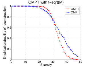
Figure 1: Average reconstruction performance of OMPT and OMP for sparse signals of length 256 in 1000 trials.

We next compare the complexity of OMPT and OMP in terms of number of inner products needed. For OMP, one can actually calculate the number of inner products, which equals $k(2d-k+1)/2$. It increases as sparsity $k$ increases, as shown in Figure 2. In contrast, we count the number of inner products performed by OMPT for 1000 trials. The average is shown in Figure 2. As one can see, it stays flat as $k$ increases and is significantly less than the number of inner products needed for OMP.

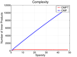
Figure 2: Average number of inner products performed by OMPT and OMP in 1000 trials.

V Conclusion

In this paper, we have analyzed a less greedy algorithm, orthogonal matching pursuit with thresholding and its performance for reconstructing sparse signals, for both noisy and noiseless cases. It replaces the expensive greedy step in orthogonal matching pursuit with a thresholding step, making it a potentially more attractive option in practice. By analysing different metrics for the sampling matrix such as the RIC, mutual coherence and global 2-coherence, we showed that although the expensive greedy step is replaced, this simplified algorithm has the same recovery performance as orthogonal matching pursuit for sparse signal reconstruction.

Appendix A Proof of expression (3)

Proof.

$$\max_{\phi_{i},i\in S}\frac{|\langle\Phi x,\phi_{i}\rangle|}{\|x\|_{2}} =\frac{\|\Phi_{S}^{T}\Phi_{S}x_{S}\|_{\infty}}{\|x_{S}\|_{2}}$$

$$=\frac{\|\Phi_{S}^{T}\Phi_{S}x_{S}\|_{\infty}}{\|(\Phi_{S}^{T}\Phi_{S})^{-1}\Phi_{S}^{T}\Phi_{S}x_{S}\|_{2}}$$

$$\geq\frac{1}{\|(\Phi_{S}^{T}\Phi_{S})^{-1}\|_{\infty,2}}.$$

Therefore,

$$\omega_{k}(\Phi)=\min_{\begin{subarray}{c}S\subset[d]\\ |S|=k\end{subarray}}\frac{1}{\|(\Phi_{S}^{T}\Phi_{S})^{-1}\|_{\infty,2}}.$$

∎

Appendix B Proof of Theorem III.5

The proof of Lemma III.3 and Lemma III.4 will need the following lemma.

Lemma B.1.

Let $\Lambda\subset[d]$ with $|\Lambda|=k$. Let $f=\Phi a+w$ with $\operatorname*{supp}(a)=\Lambda$ and $\|w\|_{2}\leq\epsilon$. In addition, assume that there exits $\Omega\subseteq\Lambda$ with $|\Omega|=m$, such that

$$\langle\Phi a,\phi_{i}\rangle=0,\mbox{ for $i\in\Lambda\setminus\Omega$}.$$

Then

$$\max_{i\in[d]\setminus\Lambda}|\langle f,\phi_{i}\rangle| \leq\nu_{k}\|a\|_{2}+\epsilon,$$

$$\max_{i\in\Lambda}|\langle f,\phi_{i}\rangle| \geq\frac{\sqrt{1-\delta_{k}}}{\sqrt{m}}\|\Phi a\|_{2}-\epsilon.$$

Proof.

For $i\in[d]\setminus\Lambda$, we have

$$|\langle f,\phi_{i}\rangle| =|\langle\Phi a+w,\phi_{i}\rangle|$$

$$\leq|\langle\Phi a,\phi_{i}\rangle|+|\langle w,\phi_{i}\rangle|$$

$$\leq\left|\sum_{j\in\Lambda}a_{j}\langle\phi_{j},\phi_{i}\rangle\right|+\|w\|_{2}\|\phi_{i}\|_{2}$$

$$\leq\|a\|_{2}\left(\sum_{j\in\Lambda}|\langle\phi_{j},\phi_{i}\rangle|^{2}\right)^{\frac{1}{2}}+\epsilon$$

$$\leq\nu_{k}\|a\|_{2}+\epsilon.$$

Taking maximum on both sides completes the proof of the first inequality.

Now for $i\in\Lambda$, we have

$$\|\Phi a\|_{2}^{2} =\langle\Phi a,\sum_{i\in\Lambda}a_{i}\phi_{i}\rangle$$

$$=\sum_{i\in\Lambda}a_{i}\langle\Phi a,\phi_{i}\rangle$$

$$=\sum_{i\in\Omega}a_{i}\langle\Phi a,\phi_{i}\rangle$$

$$\leq\sum_{i\in\Omega}|a_{i}|\cdot|\langle\Phi a,\phi_{i}\rangle|$$

$$\leq\sqrt{m}\|a\|_{2}\max_{i\in\Lambda}|\langle\Phi a,\phi_{i}\rangle|.$$

By the definition of the RIC $\delta_{k}$,

$$\max_{i\in\Lambda}|\langle\Phi a,\phi_{i}\rangle|\geq\frac{\sqrt{1-\delta_{k}}}{\sqrt{m}}\|\Phi a\|_{2}.$$

Therefore,

$$\max_{i\in\Lambda}|\langle f,\phi_{i}\rangle| =\max_{i\in\Lambda}|\langle\Phi a+w,\phi_{i}\rangle|$$

$$\geq\max_{i\in\Lambda}|\langle\Phi a,\phi_{i}\rangle|-\max_{i\in\Lambda}|\langle w,\phi_{i}\rangle|$$

$$\geq\frac{\sqrt{1-\delta_{k}}}{\sqrt{m}}\|\Phi a\|_{2}-\max_{i\in\Lambda}\|w\|_{2}\|\phi_{i}\|_{2}$$

$$\geq\frac{\sqrt{1-\delta_{k}}}{\sqrt{m}}\|\Phi a\|_{2}-\epsilon.$$

This completes the proof of the second inequality. ∎

Now we are ready to complete the proof of Lemma III.3, Lemma III.4, and Theorem III.5.

Proof of Lemma III.3.

By using Lemma B.1, assumption (12), and the fact that $\|a_{s}\|_{2}\geq\sqrt{k-s}|a_{\text{min}}|$, it is easy to derive

$$\max_{i\in[d]\setminus\Lambda}|\langle r_{s},\phi_{i}\rangle| \leq\nu_{k}\|a_{s}\|_{2}+\epsilon$$

$$<t\left(\sqrt{1-\delta_{k}}\|a_{s}\|_{2}-\epsilon\right)$$

$$\leq t\left(\|\Phi a_{s}\|_{2}-\epsilon\right)$$

$$\leq t\|r_{s}\|_{2}.$$

∎

Proof of Lemma III.4.

By using Lemma B.1, assumption (13) and the inequality

$$\sqrt{(k-s)(1-\delta_{k})}|a_{\text{min}}|\leq\sqrt{1-\delta_{k}}\|a\|_{2}\leq\|\Phi a\|_{2}$$

we have

$$\max_{i\in\Lambda}|\langle r_{s},\phi_{i}\rangle| \geq\frac{\sqrt{1-\delta_{k}}}{\sqrt{k-s}}\|\Phi a_{s}\|_{2}-\epsilon$$

$$\geq t(\|\Phi a_{s}\|_{2}+\epsilon)$$

$$\geq t\|r_{s}\|_{2}.$$

∎

Proof of Theorem III.5.

First we show that $a_{\text{ompt}}$ has the correct support.

We start with the first iteration. Combining conditions (14) and (15), Lemma III.3 and Lemma III.4, it is easy to see that OMPT is able to select and only select an atom $\phi_{i}$ with $i\in\Lambda$. Condition (14) and  (15) guarantees the existance of threshold $t$ satisfying Lemma III.3 and Lemma III.4. Lemma III.3 guarantees that OMPT will not choose any atom $\phi_{i}$ for $i\in[d]\setminus\Lambda$. While Lemma III.4 guarantees that OMPT is able to choose atoms $\phi_{i}$ with $i\in\Lambda$.

Next we argue that by repeatedly applying Lemma III.3 and Lemma III.4, we are able to correctly recover the support of $a$. In fact, in each iteration, we have the same situation as in the first iteration. In addition, the orthogonal projection step guarantees that the procedure will not repeat the atoms already chosen in previous iterations. Thus, all the correct support of the noiseless sparse signal $a$ can be recovered precisely after $k$ iterations.

Next, we will prove the error bound (16). The proof follows the idea of Theorem 5.1 in [15]. Let $a_{T}$ denote $a$ restricted to its support. Similarly, let $\Phi_{T}$ denote the dictionary $\Phi$ restricted to the support of $a$. The orthogonal projection step tells that OMPT solves for

$$\hat{a}_{T}=\operatorname*{arg\,min}_{a_{T}}\|f-\Phi_{T}a_{T}\|_{2}=\Phi_{T}^{\dagger}f$$

where $\Phi_{T}^{\dagger}$ denotes the Moore-Penrose generalized inverse of $\Phi_{T}$. Then we have

$$\hat{a}_{T} =\Phi_{T}^{\dagger}f$$

$$=\Phi_{T}^{\dagger}(\Phi a+w)$$

$$=\Phi_{T}^{\dagger}(\Phi_{T}a_{T}+w)$$

$$=a_{T}+\Phi_{T}^{\dagger}w.$$

The term $\Phi_{T}^{\dagger}w$ denotes the reconstruction error. It can be bounded by

$$\|\hat{a}_{\text{ompt}}-a\|_{2} =\|\hat{a}_{T}-a_{T}\|_{2}$$

$$=\|\Phi_{T}^{\dagger}w\|_{2}$$

$$\leq\|\Phi_{T}^{\dagger}\|_{2}\cdot\|w\|_{2}$$

$$\leq\epsilon/\sigma_{\text{min}}$$

where we bound the norm of $\Phi_{T}^{\dagger}$ by the smallest singular value $\sigma_{\text{min}}$ of $\Phi$. Now by RIP, we have $\sigma_{\text{min}}^{2}\geq 1-\delta_{k}$, and the error bound (16) follows. ∎

Appendix C Proof of Theorem III.6

Proof of Theorem III.6.

If the stopping criteria $\|r_{m}\|\leq t\|f\|$ is met, then the error estimation follow from the simple inequalities

$$\|f\|\leq\|f-f^{\epsilon}\|+\|f^{\epsilon}\|\leq\epsilon+C(\epsilon).$$

Now assume the stopping criteria $|\langle r_{m},\phi\rangle|<t\|r_{m}\|$ has been met for all $\phi\in\Phi$, and denote $G_{m}$ the approximant after $m$ iterations. Then

$$\|r_{m}\|^{2} =\langle r_{m},f-G_{m}\rangle=\langle r_{m},f\rangle$$

$$=\langle r_{m},f-f^{\epsilon}\rangle+\langle r_{m},f^{\epsilon}\rangle$$

$$\leq\|r_{m}\|\cdot\|f-f^{\epsilon}\|+C(\epsilon)\langle r_{m},\sum_{\phi_{i}\in\Phi}a_{i}\phi_{i}\rangle$$

$$\leq\epsilon\|r_{m}\|+C(\epsilon)\sum_{\phi_{i}\in\Phi}a_{i}\langle r_{m},\phi_{i}\rangle$$

$$\leq\epsilon\|r_{m}\|+tC(\epsilon)\|r_{m}\|\sum_{\phi_{i}\in\Phi}|a_{i}|$$

$$\leq\epsilon\|r_{m}\|+tC(\epsilon)\|r_{m}\|.$$

Therefore, we obtain the bound

$$\|r_{m}\|\leq\epsilon+tC(\epsilon).$$

Next, we prove the bound on the number of iterations. Suppose we are at the $k$-th iteration and have found $\phi_{i}$ such that

$$|\langle\phi_{i},r_{k-1}\rangle|\geq t\|r_{k-1}\|.$$

We now update the support

$$\Lambda_{k}=\Lambda_{k-1}\cup\{i\}.$$

and calculate the new approximant

$$G_{k}=\Phi_{\Lambda_{k}}\cdot\arg\min_{z}\|f-\Phi_{\Lambda_{k}}z\|^{2}.$$

Then

$$\|r_{k}\|^{2} =\min_{z}\|f-\Phi_{\Lambda_{k}}z\|^{2}$$

$$\leq\|r_{k-1}-\langle r_{k-1},\phi_{i}\rangle\phi_{i}\|^{2}$$

$$=\|r_{k-1}\|^{2}-\langle r_{k-1},\phi_{i}\rangle^{2}$$

$$\leq\|r_{k-1}\|^{2}-t^{2}\|r_{k-1}\|^{2}$$

$$=(1-t^{2})\|r_{k-1}\|^{2}.$$

Hence

$$\|r_{k}\|\leq(1-t^{2})^{\frac{1}{2}}\|r_{k-1}\|,$$

which implies

$$\|r_{k}\|\leq(1-t^{2})^{\frac{k}{2}}\|f\|.$$

From the stopping criteria $\|r_{m}\|\leq t\|f\|$, we know that the algorithm will stop after $m$ iterations where $m$ is the smallest integer satisfying

$$\left(1-t^{2}\right)^{\frac{k}{2}}\leq t.$$

This implies

$$m\leq\frac{2\ln t}{\ln(1-t^{2})}.$$

∎

References

- [1] E. J. Candes, J. Romberg, and T. Tao, “Robust uncertainty principles: exact signal reconstruction from highly incomplete frequency information,” IEEE Trans. on Inf. Theory, vol. 52, no. 2, pp. 489–509, 2006.
- [2] E. J. Candes and T. Tao, “Near-Optimal Signal Recovery From Random Projections: Universal Encoding Strategies?” IEEE Trans. on Inf. Theory, vol. 52, no. 12, pp. 5406–5425, 2006.
- [3] D. L. Donoho, “Compressed sensing,” IEEE Trans. Inform. Theory, vol. 52, no. 4, pp. 1289–1306, 2006.
- [4] C. Shannon, “Communication in the presence of noise,” Proceedings of the Institute of Radio Engineers (IRE), vol. 37, pp. 10–21, 1949.
- [5] E. J. Candes and T. Tao, “Decoding by linear programming,” IEEE Trans. on Inf. Theory, vol. 51, no. 12, pp. 4203–4215, 2005.
- [6] E. J. Candes, “The restricted isometry property and its implications for compressed sensing,” Comptes Rendus Mathematique, vol. 346, no. 9-10, pp. 589 – 592, 2008.
- [7] S. Foucart and M.-J. Lai, “Sparsest solutions of underdetermined linear systems via -minimization for ,” Applied and Computational Harmonic Analysis, vol. 26, no. 3, pp. 395 – 407, 2009.
- [8] S. Foucart, “A note on guaranteed sparse recovery via -minimization,” Applied and Computational Harmonic Analysis, vol. 29, no. 1, pp. 97 – 103, 2010.
- [9] T. Cai, L. Wang, and G. Xu, “Shifting inequality and recovery of sparse signals,” Signal Processing, IEEE Transactions on, vol. 58, no. 3, pp. 1300–1308, 2010.
- [10] ——, “New bounds for restricted isometry constants,” Information Theory, IEEE Transactions on, vol. 56, no. 9, pp. 4388–4394, 2010.
- [11] Q. Mo and S. Li, “New bounds on the restricted isometry constant,” Applied and Computational Harmonic Analysis, vol. 31, no. 3, pp. 460 – 468, 2011.
- [12] A. C. Gilbert, S. Muthukrishnan, and M. J. Strauss, “Approximation of functions over redundant dictionaries using coherence,” in Proceedings of the fourteenth annual ACM-SIAM symposium on Discrete algorithms, ser. SODA ’03. Philadelphia, PA, USA: Society for Industrial and Applied Mathematics, 2003, pp. 243–252.
- [13] D. L. Donoho, M. Elad, and V. N. Temlyakov, “Stable recovery of sparse overcomplete representations in the presence of noise,” USC, Tech. Rep. 04:06, 2004.
- [14] J. Tropp, “Greed is good: algorithmic results for sparse approximation,” Information Theory, IEEE Transactions on, vol. 50, no. 10, pp. 2231–2242, 2004.
- [15] D. L. Donoho, M. Elad, and V. N. Temlyakov, “Stable recovery of sparse overcomplete representations in the presence of noise,” IEEE Trans. Inform. Theory, vol. 52, no. 1, pp. 6–18, 2006.
- [16] D. Needell and J. Tropp, “Cosamp: Iterative signal recovery from incomplete and inaccurate samples,” Applied and Computational Harmonic Analysis, vol. 26, no. 3, pp. 301 – 321, 2009.
- [17] W. Dai and O. Milenkovic, “Subspace pursuit for compressive sensing signal reconstruction,” Information Theory, IEEE Transactions on, vol. 55, no. 5, pp. 2230–2249, 2009.
- [18] D. Needell and R. Vershynin, “Signal recovery from incomplete and inaccurate measurements via regularized orthogonal matching pursuit,” Selected Topics in Signal Processing, IEEE Journal of, vol. 4, no. 2, pp. 310–316, 2010.
- [19] T. Blumensath and M. E. Davies, “Iterative hard thresholding for compressed sensing,” Applied and Computational Harmonic Analysis, vol. 27, no. 3, pp. 265 – 274, 2009.
- [20] S. Foucart, “Hard thresholding pursuit: An algorithm for compressive sensing,” SIAM J. Numer. Anal., vol. 49, no. 6, pp. 2543–2563, Dec. 2011.
- [21] D. Donoho, Y. Tsaig, I. Drori, and J.-L. Starck, “Sparse solution of underdetermined systems of linear equations by stagewise orthogonal matching pursuit,” Information Theory, IEEE Transactions on, vol. 58, no. 2, pp. 1094–1121, Feb 2012.
- [22] M. Yang and F. de Hoog, “New coherence and rip analysis for weak orthogonal matching pursuit,” in Statistical Signal Processing (SSP), 2014 IEEE Workshop on, June 2014, pp. 376–379.
- [23] V. Temlyakov, Greedy Approximation. Cambridge University Press, 2011.
- [24] D. Donoho and X. Huo, “Uncertainty principles and ideal atomic decomposition,” Information Theory, IEEE Transactions on, vol. 47, no. 7, pp. 2845 –2862, nov 2001.
- [25] M. Elad and A. M. Bruckstein, “A generalized uncertainty principle and sparse representation in pairs of bases,” IEEE Trans. Inform. Theory, vol. 48, no. 9, pp. 2558–2567, 2002.
- [26] D. L. Donoho and M. Elad, “Optimally sparse representation in general (nonorthogonal) dictionaries via minimization,” Proceedings of the National Academy of Sciences, vol. 100, no. 5, pp. 2197–2202, 2003.
- [27] R. Gribonval and M. Nielsen, “Sparse representations in unions of bases,” IEEE Trans. Inform. Theory, vol. 49, no. 12, pp. 3320–3325, 2003.
- [28] Y. Eldar and H. Rauhut, “Average case analysis of multichannel sparse recovery using convex relaxation,” Information Theory, IEEE Transactions on, vol. 56, no. 1, pp. 505–519, 2010.
- [29] M. Davenport and M. Wakin, “Analysis of orthogonal matching pursuit using the restricted isometry property,” Information Theory, IEEE Transactions on, vol. 56, no. 9, pp. 4395–4401, 2010.
- [30] S. Huang and J. Zhu, “Recovery of sparse signals using omp and its variants: convergence analysis based on rip,” Inverse Problems, vol. 27, no. 3, 2011.
- [31] E. Liu and V. Temlyakov, “The orthogonal super greedy algorithm and applications in compressed sensing,” Information Theory, IEEE Transactions on, vol. 58, no. 4, pp. 2040–2047, 2012.
- [32] J. Wang and B. Shim, “On the recovery limit of sparse signals using orthogonal matching pursuit,” Signal Processing, IEEE Transactions on, vol. 60, no. 9, pp. 4973–4976, Sept 2012.
- [33] Q. Mo and Y. Shen, “A remark on the restricted isometry property in orthogonal matching pursuit,” Information Theory, IEEE Transactions on, vol. 58, no. 6, pp. 3654–3656, 2012.
- [34] T. Zhang, “Sparse recovery with orthogonal matching pursuit under rip,” Information Theory, IEEE Transactions on, vol. 57, no. 9, pp. 6215–6221, Sept 2011.
- [35] M. Duarte and Y. Eldar, “Structured compressed sensing: From theory to applications,” Signal Processing, IEEE Transactions on, vol. 59, no. 9, pp. 4053–4085, Sept 2011.
- [36] H. Rauhut, “Compressive sensing and structured random matrices,” in Theoretical Foundations and Numerical Methods for Sparse Recovery, ser. Radon Series Comp. Appl. Math., M. Fornasier, Ed. deGruyter, 2010, vol. 9, pp. 1–92, corrected Version (April 4, 2011): Noncommutative Khintchine inequality for Rademacher chaos (Theorem 6.22) corrected, Proof of Theorem 9.3 corrected. Proof of Lemma 8.2 corrected.
- [37] M. Yang, “Greedy algorithms in approximation theory and compressed sensing,” Ph.D. dissertation, University of South Carolina, Columbia, SC, USA, 2011, aAI3469193.
- [38] V. Temlyakov, “Relaxation in greedy approximation,” Constructive Approximation, vol. 28, no. 1, pp. 1–25, 2008.
- [39] V. N. Temlyakov, “Greedy approximation,” Acta Numer., vol. 17, pp. 235–409, 2008.