Dipole anisotropy in sky brightness and source count distribution in radio NVSS data
Abstract
We study the dipole anisotropy in number counts and flux density weighted number counts or sky brightness in the NRAO VLA Sky Survey (NVSS) data. The dipole anisotropy is expected due to our local motion with respect to the CMBR rest frame. We analyse data with an improved fit to the number density, , as a function of the flux density , which allows deviation from a pure power law behaviour. We also impose more stringent cuts to remove the contribution due to clustering dipole. In agreement with earlier results, we find that the amplitude of anisotropy is significantly larger in comparison to the prediction based on CMBR measurements. The extracted speed is found to be roughly 3 times the speed corresponding to CMBR. The significance of deviation is smaller, roughly 2 , in comparison to earlier estimates. For the cut, mJy, the speed is found to be Km/s using the source count analysis. The direction of the dipole anisotropy is found to be approximately in agreement with CMBR. We find that the results are relatively insensitive to the lower as well as upper limit imposed on the flux density. Our results suggest that the Universe is intrinsically anisotropic with the axis of anisotropy axis pointing roughly towards the CMBR dipole direction. Finally we present a method which may allow an independent extraction of the local speed and an intrinsic dipole anisotropy, provided a larger data set becomes available in future.
keywords:
radio galaxies: high-redshift, galaxies: active1 Introduction
The observed dipole anisotropy in the Cosmic Microwave Background Radiation (CMBR) is generally interpreted in terms of the motion of the solar system with respect to the CMBR rest frame. The corresponding speed is found to be (369 0.9 Km s-1) in the direction, , in galactic coordinates [1, 2]. In J2000 equatorial coordinates, the direction parameters are , . We expect that, at large distance scales, galaxies would be distributed isotropically with respect to the CMBR rest frame. However, due to Doppler and aberration effect, they would show an anisotropic distribution [3] in the solar rest frame. The dipole anisotropy in radio sources should be observable both in number counts and flux density weighted number counts (sky brightness) of sources at high redshifts. The resulting anisotropy has been probed in radio surveys by many authors [4, 5, 6, 7, 8, 9]. Using the NRAO VLA Sky Survey (NVSS) [10], [5] reported a positive detection of dipole anisotropy in the radio source count with the direction in reasonable agreement with CMBR. The speed was found to be roughly 1.5 to 2 times larger in comparison to that extracted from the CMBR dipole. In an independent analysis of the same data, using both number counts and sky brightness, [7] reported a much larger value of the local velocity ( 400 Km s-1), which is roughly four times larger than the prediction from CMBR observations. The direction was found to be consistent with the CMBR dipole. The results using number counts and sky brightness agreed with one another within errors, with the sky brightness based analyses yielding a larger value. Furthermore, [8, 9] also find a dipole anisotropy much larger than the CMBR prediction.
The current situation with radio analysis is clearly puzzling. All the four analysis [5, 7, 8, 9] find direction in agreement with the CMBR, but disagree on the extracted speed. Although, [5] claim results roughly consistent with CMBR, the large amplitude found in [7] suggests a potential violation of the cosmological principle. Ref. [8] attribute their deviation from CMBR predictions to observational bias. Ref. [9] attribute the different results obtained in literature to difference in the estimators used. In the present paper we revisit this problem in an attempt to get a consistent result.
In contrast to the above results, the Planck team finds further evidence that CMBR dipole arises dominantly due to local motion [11]. A dipole anisotropy has also been observed in the diffuse x-ray background [12]. In this case, both the amplitude and direction are found to be consistent with the prediction based on the CMBR dipole. Furthermore several authors have observed that the local galaxy distribution shows a dipole whose direction shows reasonable agreement with the CMBR dipole [13, 14, 15]. However the magnitude of this clustering dipole does not show convergence even up to distances of order 300 Mpc. It appears to us that the evidence for CMBR dipole being a kinematic effect is quite strong. All studies of dipole in galaxy surveys also give a direction close to CMBR. However the amplitude of the dipole in these surveys is still uncertain. Theoretically it is possible that large scale structures might show an anisotropy not consistent with that expected from kinematic effects. A possible model in which this can arise is discussed in [16, 17, 18]. In this case it is assumed that the Universe is anisotropic during the pre-inflationary phase of its evolution. The perturbations generated during this phase re-enter the horizon at late times and can affect structure formation, while having negligible effect on CMBR. Hence in this case large scale structures can show an intrinsic dipole pattern even if the CMBR is isotropic, up to kinematic effects.
The NVSS data set does not cover the sky evenly. Further cuts imposed on the data that remove the galactic plane and the local structure dipole exacerbate this problem. There are various approaches to analyse data that covers the sky partially. We treat the masked regions by filling them randomly by data extracted from the remaining pixels. This preserves the distribution of data in the masked regions. We extract the dipole from data by making a spherical harmonic decomposition. This procedure differs from that adopted in [5] who analyze masked sky data directly. Singal [7] adopts a different strategy of dropping sources that are diametrically opposite to the NVSS gap so as to eliminate a dipole structure introduced by the gap. We find the full sky analysis convenient since it allows us to probe the dipole directly. Furthermore any bias that might be generated by random filling can be determined by simulations and removed from the final result.
We independently extract the dipole anisotropy from number counts and sky brightness using spherical harmonic decomposition. We also report the statistical significance of the extracted dipole anisotropy. This important parameter has not been reported in any of the earlier papers which only list the sigma value with which the extracted dipole differs from that predicted by CMBR. The bias in the extracted magnitude and direction of velocity, generated due to partial sky data, is computed by simulations and subtracted from the final results. We point out that a pure power law does not provide a good to the number density of sources, , as a function of the flux density, . Hence we consider an improved fit which accounts for the deviation of number density from a pure power law. This provides a more reliable extraction of the local velocity from the data. Furthermore, we show that in this case the kinematic dipole is different for number counts in comparison to flux weighted number counts. Earlier results indicate the presence of an intrinsic dipole anisotropy in the number count distribution [7]. We show that, with sufficient data, the improved fit allows an independent extraction of the local velocity and the intrinsic dipole anisotropy, which might be present in data. Finally, we present a method based on flux density per source, which can be used even in the case of uneven distribution of source counts. This allows an independent extraction of the local velocity. This method is found to be not effective for the present data set but may prove useful when additional data becomes available.
The dipole anisotropy in the NVSS data may also get contributions from sources in the local supercluster, which are expected to show a dipole with prefered direction close to the CMBR dipole. This contribution has to be eliminated from data. We follow two different procedures for this purpose. First we eliminate the known local sources using standard catalogues. This procedure was also employed in [5]. For imposing this cut, we also use recent catalogues of points sources which have become available since the publication of [5]. Alternatively we impose an additional cut which eliminates the supergalactic plane [7]. In this case we try several different cuts, corresponding to supergalactic latitude, and .
We also impose a cut in order to eliminate several extended and bright radio sources. In the NVSS survey these would be misidentified as a cluster of very large number of sources over sky regions of size greater than a degree [5] and hence may introduce significant error in the extracted dipole. This cut was imposed in [5] where the authors identified a total of 22 such regions. Such regions would introduce spurious clustering in the data and have to be removed. This cut was not imposed in subsequent analysis of the data [7, 8, 9]. We determine the sensitivity of the extracted dipole to this cut in order to make a proper comparison of results with those obtained in [5].
The results obtained by [7] suggest the possibility that the Universe may be intrinsically anisotropic with the preferred axis approximately in the direction of the CMBR dipole. There already exist considerable evidence in favor of such a hypothesis [19]. The radio polarization offset angles with respect to the galaxy axis show a dipole anisotropy with preferred axis closely aligned with CMBR dipole [20]. The Cosmic Microwave Background Radiation (CMBR) quadrupole and octupole [21] as well as the two point correlations in the quasar optical polarizations [22, 23, 24] also indicate a preferred axis closely aligned with CMBR dipole axis [19, 25]. Another interesting effect which has been observed in CMBR is the hemispherical anisotropy [26]. This effect is generally interpreted in terms of dipole modulation in the temperature field [27, 28]. This dipole modulation effect, however, has not been observed in [29, 30] in NVSS data. A search for quadrupolar power anisotropy also yields a null result [31]. We point out that this dipole modulation effect or the quadrupolar anisotropy is not related to the dipole anisotropy we study in the present paper. In particular, the axes of the two dipoles are completely different.
2 Theory
The absolute cosmological frame of reference can be determined by observing the dipole anisotropy of CMBR or radio data. The assumption here is that there is no intrinsic dipole anisotropy and the observed dipole is purely due to local motion which causes Doppler and aberration effect. The very first attempt to determine the local motion began with [3]. An observer moving with a velocity (), sees the sky brighter in forward direction due to Doppler boosting and aberration effect. The flux density of radio sources follows a power-law dependence on frequency , , with [3]. For an observer moving with a velocity , the Doppler shift in the frequency () is , where
| (1) |
at leading order. This leads to [3],
| (2) |
at a fixed frequency in observer frame. Furthermore, the aberration effect changes the solid angle in the direction of motion .
Let us denote the differential number count per unit solid angle per unit flux density by , where are the polar angles corresponding to the direction of observation. Assuming isotropy, we have, in the rest frame,
| (3) |
where we have assumed a power law form for and the flux density is in units of mJy. Here is the number of sources in a small bin, in solid angle and flux density. The anisotropy due to kinematic dipole is small. Hence we may fit this functional form to data, ignoring this anisotropy. The best fit to data in the flux density range, 20 mJy 1000 mJy, over the entire sky, is shown in Fig. 1. In this figure denotes the distribution in Eq. 3. The fit parameters are determined by using the “Minuit” Minimization Package provided by the CERN ROOT software. The program applies the minimization procedure on binned data. Here we use uniform bins of width 0.1 mJy. The values of for different cuts on the flux density are given in Table 1. For the case of mJy, we find that for 7416 degrees of freedom. For a small bin size of 0.1 mJy, we find that there are several bins which have no sources. These are removed by the fitting program. The fit parameters show very little dependence on the choice of bin size. For example, if we determine the fit parameters using only 20 bins, we obtain for the cut mJy. Such a mild change has negligible effect on our final results.
| 10 | 20 | 30 | 40 | 50 | |
|---|---|---|---|---|---|
| 1.168 |
It can be seen from Fig. 1 that a pure power law, does not provide a good fit to data. A much better fit is provided by allowing the spectral index to depend on . We discuss this improved fit in section 2.1, where we also develop the formalism to extract the kinematic dipole for such a modified functional form. Here we review the standard treatment for a pure power law fit, first developed in [3].

Let represent the number of sources in the bin . We have,
where is number of sources in the corresponding bin in rest frame. We, therefore, obtain,
| (4) |
Substituting for , we obtain,
| (5) |
Integrating over from to , we obtain the standard result [3],
| (6) |
Hence Doppler boosting and aberration, at leading order in , produces a dipole anisotropy in source count, given by,
| (7) |
In [3] it has been pointed out that to measure the dipole anisotropy at significance level one needs to have more than radio sources. However such a large catalogue was not available at that time. The authors analyzed 4C catalogue data (4844 sources), and determined the local velocity as Km s-1.
We next generalize this calculation to sky brightness, . This is defined as the number counts weighted by flux density, i.e.,
| (8) |
We have,
| (9) |
where we have used Eq. 4. This leads to,
| (10) |
The integral of this quantity over from to is divergent for . Hence we also impose an upper limit, , as done in the actual data analysis. We obtain, after integration,
| (11) |
The final result is same as for number counts. The dipole anisotropy, , in is also given by the same formula as ,
| (12) |
This provides an independent method to compute the velocity of the solar system with respect to the cosmological rest frame.
Earlier analysis [7], suggest the presence of an intrinsic dipole anisotropy in the radio data. Hence let us assume the following form for the observed .
| (13) |
where represents the intrinsic dipole anisotropy in the number counts. Let us next assume that the intrinsic anisotropy in the sky brightness is caused entirely by the intrinsic anisotropy in the source distribution. This assumption can be directly tested by exploring the anisotropy in the flux density per source, denoted by . This measure would not be affected by the intrinsic dipole in number counts. Furthermore the kinematic dipole also does not contribute to this measure since it is same both for number counts and flux weighted number counts. Hence, with our assumptions, should not show a significant signal of anisotropy,
2.1 An improved fit
We next generalize the calculation to a somewhat better fit to data, which takes into account the deviation from a pure power law behaviour. We assume the following form of ,
| (14) |
where, as before, the flux density is in units of mJy. This functional form significantly improves the fit to data, as can be seen in Fig. 1. We use this fit to extract the local velocity from data. The fit parameters are given in Table 2 for different cuts on the flux density. In this case the is found 6481 for 7415 degrees of freedom for the cut mJy. Following the steps described above, we obtain, at leading order in ,
| (15) |
where, . Integrating over from to , we obtain,
| (16) | |||||
where
| (17) |
| (18) | |||||
| (19) |
and
| (20) |
The resulting functional form can be fitted to data, after numerically performing the integrals, and , in order to extract the local velocity.
| 10 | 20 | 30 | 40 | 50 | |
|---|---|---|---|---|---|
| 0.0478 | |||||
| 0.1199 | 0.1307 | 0.1360 | 0.1309 | 0.1134 | |
| 3.34 | 3.55 | 3.70 | 3.82 | 3.94 | |
| 3.82 | 3.95 | 4.04 | 4.11 | 4.16 |
For the case of sky brightness we obtain,
| (21) |
where
| (22) |
| (23) | |||||
| (24) |
and
| (25) |
We find that in this case the kinematic dipole contributes differently to number counts and to sky brightness. The difference, however, is small. Nevertheless, it might be useful in future in order to independently extract the intrinsic and kinematic dipole from data. This may be accomplished as follows. Let the observed dipole in number counts and sky brightness be represented as
| (26) |
and
| (27) |
where we have again assumed that the intrinsic anisotropy in sky brightness is same as that in number counts. We obtain,
| (28) |
Using the extracted local velocity we can determine the intrinsic dipole from Eq. 26. Alternatively we may determine the anisotropy in the flux density averaged over the number counts, . The dipole in this variable is given by,
| (29) |
where we have used Eqs. 26 and 27. By analysing the variable we can directly extract , which can be used in Eq. 26 to extract .
3 The Data
The NRAO VLA Sky Survey (NVSS) [10] is a radio continuum survey covering the entire northern sky, . It operates at the frequency of 1.4 GHz. The NVSS catalogue contains 1773484 radio sources. Following [5] we impose various cuts on data. We only include sources with flux density lying within the range and , where mJy. The data with lower limit mJy is not expected to be reliable [5]. Hence results for this cut should be interpreted with caution. The upper limit, , is generally taken to be 1000 mJy. However we also determine how the results change if it is changed to 900 mJy. We remove sources lying within the galactic latitude . After this cut, the masked region constitutes 38% of the sky. We test the sensitivity of our results to this cut on the galactic latitude. Furthermore, we remove the clustering dipole [5], i.e. sources which might belong to the local supercluster. This is accomplished by removing sources within 30 arcsec of known nearby galaxies as listed in [32] and in the third reference catalogue of bright Galaxies (RC3) [33, 34]. These catalogues contain 23011 and 18351 sources respectively. This cut removes a total of 13597 sources from the NVSS data set. The data set obtained after removal of these sources is labelled as set (a). Besides these catalogues, we also use recent catalogues of local point sources [36, 35, 37] which have become available since the publication of [5]. These contain a total of 617 [36], 43526 [35] and 928352 [37] sources. These catalogues lead to a removal of additional 64475 sources from the NVSS data set, leaving a total of 1695412 sources. An additional cut which removes the 22 sites of bright and extended radio sources, identified in [5] and discussed in section 1, leaves a total of 1674536 sources. These 22 sites are filled by randomly generated isotropic data, following the procedure adopted in [5]. The data set obtained after imposing this more stringent cut is called set (b). We extract the dipole vector both for set (a) and set (b). Using all of the above cuts we have about sources remaining in the data set. We determine the sensitivity of our results to the exclusion radius around each source. In particular we determine how the results change if this radius is varied from to .
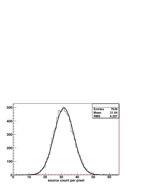
We use HEALPix111http://healpix.jpl.nasa.gov/ to generate the angular position on the sky with the resolution parameter . The angular size of a pixel for is roughly . Using this resolution we fill the map with randomly generated data, as described below. The distribution of number counts in each pixel, Fig. 2, is reasonably well described by a Gaussian. We do not find any pixel with no sources in the unmasked regions. We also determine the sensitivity of our results to the choice of pixel size.
4 Procedure
Let , represent the number count or sky brightness () as a function of the polar coordinates . Here we use J2000 equatorial system with equal to the right ascension (RA) and . We rewrite this field as , so that represents the fluctuations in this field. To study the correlation of this field we expand in spherical harmonics, , as,
| (30) |
where, are the harmonic coefficients. The power, , in each multipole is given by,
| (31) |
A significant value of indicates anisotropy at a scale radian. In particular, represents the dipole term which is related to the dipole amplitude, , as [8],
| (32) |
In the present paper we are interested only in the dipole. Hence we do not discuss higher multipoles in this paper.


4.1 Analysis Method and Bias simulation
We do not have data for and we impose a cut in order to eliminate the region around the Galactic plane. After imposing this cut, we have data only over 62% of the sky area. The dipole power of the real data is obtained by filling the empty pixels isotropically by randomly generated data and computing the corresponding full sky power. The distribution of data in the masked region is same as real data, as long as we ignore the dipole which might be present in the real data. We generate a total of 1000 realizations of real map by filling the empty pixels with different random samples. The source distribution of the masked map for the cut mJy is shown in Fig. 3. In this figure we also show a full sky map, with the masked regions filled by a particular realization of the randomly generated data. The mean dipole power, , and the mean direction parameters , are computed from the 1000 realizations of the real map. The error in these parameters is computed by simulations, as described below. The dipole extracted in this manner would differ from that extracted from the full sky map, i.e. if real data in all the pixels were available, by some constant [7], which would depend on the mask used for data. Similarly the extracted values of the direction would also contain a bias. Let represent the true direction of the dipole and the dipole extracted after filling the masked region by isotropic random samples. The bias in the angles is given by, and . We calculate the constant and the bias in direction by simulations. The bias corrected value of the dipole power, , is given by, . Similarly the angle parameters of the dipole direction are given by, and .


The random samples for number counts are generated by using the distribution shown in Fig. 2, which is extracted directly from data. This is the distribution of number of sources per pixel, as explained in section 3. For the intensity dipole we also require the flux density of sources in the random sample. This is generated by using the flux density distribution, Fig. 1, of real data. Using a random sample of number counts per pixel, we randomly allocate the values of flux density of real sources to each source in the simulated data. This yields a random isotropic sample, which has same statistical properties as the NVSS catalog.
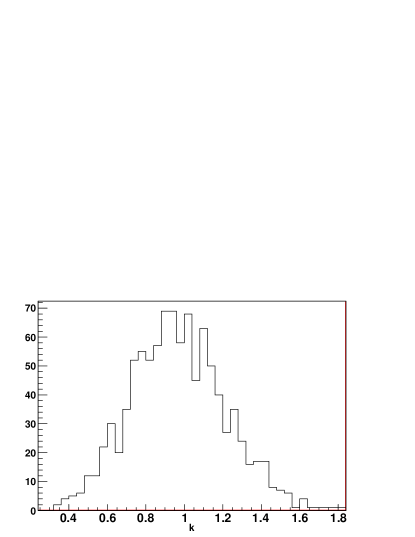
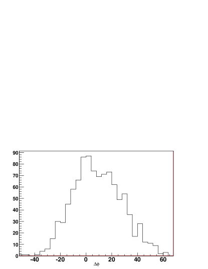
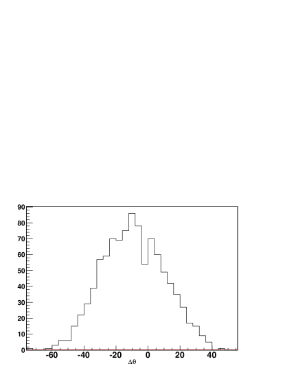
The bias is computed by simulating a random sample of radio sources which has the same distribution as the real sources. The simulated sample has a dipole of approximately the same strength as seen in real NVSS data in roughly the same direction as observed. The pixels in the masked regions, and Galactic plane within the latitude , are filled isotropically, as in the case of real data. This provides a particular random sample with same characteristics as the real data. The results obtained from 1000 realizations for sky brightness and number counts are shown in Fig. 4, 5 respectively. These figures show the distribution of , and . The resulting mean values of , and over 1000 random samples represent their bias values. The extracted values of mean and standard deviation of , and , both for source count and sky brightness, are given in Table 3 for different cuts on . The mean values of are not too different from unity and the extracted bias in angles is close to zero. Hence the required bias correction is relatively small. The standard deviations, given in Table 3, provide a reliable estimate of the statistical errors in the dipole parameters, as discussed below.

| Sources | Source Counts | Sky Brightness | |||||
|---|---|---|---|---|---|---|---|
| (deg) | (deg) | (deg) | (deg) | ||||
| 10 | 428210 | ||||||
| 20 | 240772 | ||||||
| 30 | 165206 | ||||||
| 40 | 124173 | ||||||
| 50 | 98295 | ||||||
The significance of dipole is calculated as follows. We generate 10000 full sky isotropic random realizations of the NVSS data set. The random data is generated by the procedure described above. We calculate the dipole power, , of each of these random samples. The significance is equal to the probability that a random sample can generate a dipole of strength larger than that seen in real data. We compute this by determining the number of random samples, whose dipole power exceeds that seen in real data. Here we use the data dipole power, , without applying bias correction since it provides a conservative estimate of significance. The results are presented by converting this probability into the sigma significance value. For example, two sigma corresponds to a probability of 4.55%.
4.2 Error Estimation
The bias simulations discussed above also give us a reliable estimate of statistical errors in dipole amplitude and angle variables– and . These simulations take in account all sources of random fluctuations, which include intrinsic fluctuations as well as those generated due to random filling of masked regions, that can affect the extracted dipole. Thus the standard deviation in the bias factor , and directly gives an estimate of errors in dipole parameters. The fractional error in equals the fractional error in extracted dipole amplitude. Additionally, the error in and is equal to and respectively.
5 Results
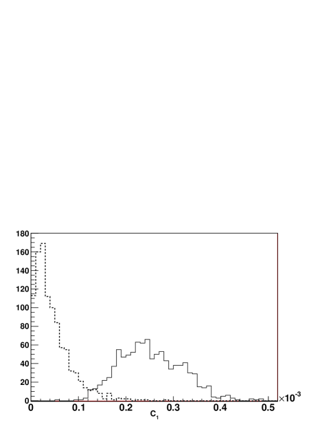
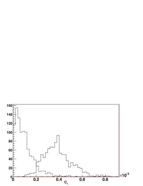
In Fig. 6, we show the distribution of dipole power for real data as well as randomly generated simulated data with the cut mJy for the case of number counts. The corresponding graphs for sky brightness, , are shown in Fig. 7. The sky brightness is obtained by summing the flux density over all sources in a particular pixel. The extracted values of for various cuts (S10, 20, 30, 40, 50 mJy) for the case of number count and sky brightness, , are given in Tables 4, 5 for set (a). In most cases we impose an upper limit mJy on the flux density of a source. We also test the sensitivity of our results to this upper limit. The cut mJy is not supposed to be reliable due to the bias in number counts [5]. We show it here mainly for comparison to see how the results change as we push the limit on to lower values. Hence the results for this cut should be interpreted cautiously. The significance of the detected dipole anisotropy as well as the direction parameters are also shown. The primes on these parameters indicate that these have not been corrected for bias. We find that the significance of the dipole anisotropy in number counts ranges from 3.2 to 2.7 for different cuts. For the sky brightness the maximum significance is found to be about 2.6 .
| significance | (deg) | (deg) | |||
|---|---|---|---|---|---|
| 10 | 3.0 | ||||
| 20 | 3.2 | ||||
| 30 | 3.0 | ||||
| 40 | 2.7 | ||||
| 50 | 2.8 |
| significance | (deg) | (deg) | |||
|---|---|---|---|---|---|
| 10 | 2.7 | ||||
| 20 | 2.6 | ||||
| 30 | 2.6 | ||||
| 40 | 2.4 | ||||
| 50 | 2.3 |
In Tables 4, 5, we also list the mean dipole power, , obtained from isotropic random samples. It is clear that it is possible to detect a dipole anisotropy in real data only if its power is significantly higher than . For comparison, the power expected due to kinematic dipole corresponding to Km/s is , assuming a pure power law fit, Eq. 3, with . This is smaller than the power corresponding to random isotropic samples for most of the cases studied in Tables 4, 5. The only exception is the cut, mJy, for number counts. In this case also the random power is comparable to the power expected due to CMBR dipole. Hence we find that it is not possible to extract a significant signal of dipole anisotropy in NVSS data, if the only signal present in data arises due to the kinematic effect, as expected from CMBR observations [6].
After correcting for bias, the extracted dipole amplitudes, and , corresponding to number counts and sky brightness respectively, are shown in Tables 6, 7. The extracted speed of the solar system, assuming that dipole is entirely a kinematic effect, and angles , after correcting for bias, are also shown. The speed is extracted by using the improved fit, Eq. 14. The values of in Eq. 14, obtained by directly fitting the data sample, are given in Table 2. Using the pure power law fit, we find that the extracted speed is similar to that obtained by the improved fit. In Tables 6, 7 we give results for both the data sets (a) and (b). The data sets are described in section 3. We point out that set (b) is obtained after imposing a more stringent cut on the data for removal of local sources. We find that the extracted dipole amplitude for set (b) is smaller in comparison to set (a) by about 20% for the case of number counts. However the change is much smaller for sky brightness. In most cases, the final result is still more than three times the speed expected from CMBR dipole. The shift in the direction parameters from set (a) to set (b) is found to be well within errors.
We find that, for the case of number counts, the results show some variation with the cut on flux density. However the change is not very large and the results agree within errors, as long as we ignore the cut mJy. For such small values of flux density, the data set is known to have uneven distribution of source counts due to non-uniform sampling [5]. The corresponding parameters, extracted using sky brightness, are found to be comparatively insensitive to the cut imposed. The angle parameters show almost no change, whereas the extracted speed varies between to , including the cut mJy. The extracted speed is found to be about times the expectation from CMBR observations. The significance of the difference is about for set (a), both for number counts and sky brightness. For set (b) the significance of difference is roughly 2 . Hence the data sample is not consistent with the CMBR dipole. However the deviation is found to be less significant in comparison to earlier results [7, 8, 9]. Our result indicates the presence of an intrinsic dipole anisotropy which cannot be explained in terms of local motion.
We next test the sensitivity of our results to the choice of pixel size. Using the HEALPix resolution parameter, , we find that results for dipole parameters agree with those obtained with within errors. In particular, the results for brightness show very little sensitivity to the choice of pixel size. The extracted dipole power for number counts, however, is found to be systematically larger by 3% to 7% for different cuts on . We have also tested how the results change if we increase the exclusion radius around each masked local source from 30 arcsecs to 45 arcsecs. The results for number counts change by less than 1 percent for all the cuts considered. For sky brightness, the change is less than 3 percent for all cases. Hence we find that the extracted dipole parameters are not very sensitive to the choice of exclusion radius.
| Set | |||||
|---|---|---|---|---|---|
| (Km/s) | RA (deg) | DEC (deg) | |||
| 10 | (a) | ||||
| (b) | |||||
| 20 | (a) | ||||
| (b) | |||||
| 30 | (a) | ||||
| (b) | |||||
| 40 | (a) | ||||
| (b) | |||||
| 50 | (a) | ||||
| (b) | |||||
| Set | |||||
|---|---|---|---|---|---|
| (Km/s) | RA (deg) | DEC (deg) | |||
| 10 | (a) | ||||
| (b) | |||||
| 20 | (a) | ||||
| (b) | |||||
| 30 | (a) | ||||
| (b) | |||||
| 40 | (a) | ||||
| (b) | |||||
| 50 | (a) | ||||
| (b) | |||||
The results obtained by using sky brightness are found to be relatively insensitive to the lower limit imposed on the flux density. However it is possible that these results might be sensitive to the upper limit, especially since the integral of , Eq. 10, using a pure power law fit, 3, diverges if the limits of integration are taken to be to . Hence it is important to test the sensitivity of our results to the upper limit also in this case. The results obtained using an upper limit mJy, instead of mJy used earlier, show negligible change. The dipole amplitude for this case is found to be, , , , , , for the cuts, mJy respectively for set (a). We find that the dipole amplitude changes by only about 5 percent in comparison to the results shown in Table 7. The direction parameters show even smaller change. Hence we do not find strong sensitivity to either the upper limit or the lower limit in this case.
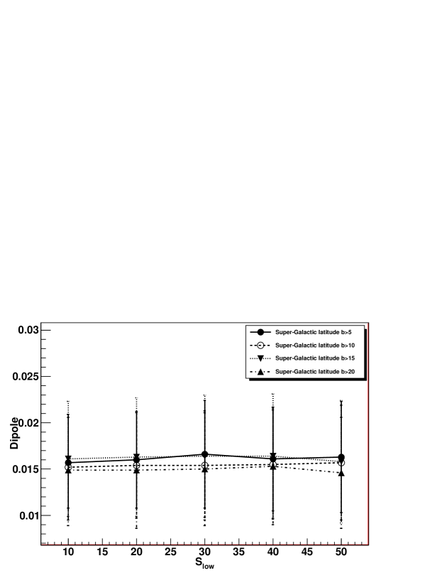
An alternative procedure for the removal of local sources is to mask the supergalactic plane. We expect that the local sources would be dominantly clustered close to this plane. Hence their contribution would be significantly reduced if this plane is masked out. In Fig. 8 we show the dipole amplitude for different cuts on the flux density, , after masking the supergalactic plane. In this case we do not remove the local sources using known catalogues. We expect that their effect would be minimized by the cut on supergalactic plane. The results are shown after masking regions corresponding to supergalactic latitude, and . In this analysis the galactic plane, corresponding to , is also masked. We find that the results obtained are consistent with those shown in Tables 6 and 7. The dipole, both for the number counts and sky brightness, does not show any particular trend. The overall dependence on the cut on is well within errors on the dipole amplitude. We point out that the masked region for the cut becomes very large. For example, for the cut, , we find that 60% of the sky gets eliminated. In comparison, for , 49% gets eliminated. For large masks, our procedure of bias correction may not be very reliable. Hence some of these results, particularly for cuts, , should be interpreted with caution. In any case it is satisfying that the results using this approach are comparable to those obtained in Tables 6 and 7 by directly removing local sources using standard catalogues.


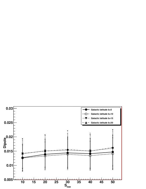
We next determine the sensitivity of our results to the cut on the galactic plane. In this case we use data set (b), i.e. we impose a stringent cut to remove the local sources. In Fig. 9, we show the change in dipole amplitude as we mask the galactic plane corresponding to latitude, and . We again do not find any particular trend in the dipole amplitude, both for number counts and sky brightness, as we increase from to . For all the five cuts on the dependence on the cut on galactic latitude is relatively mild. We also consider a galactic cut which depends on the galactic longitude in order to remove a larger region near the galactic center. In this case we exclude the region corresponding to, for , and for other values of . In this case we find that the dipole amplitude is and for the cuts mJy respectively for the case of number counts. The corresponding dipole amplitude for sky brightness is . Again by comparing with Fig. 9, we find results consistent with other cuts used to eliminate galactic plane. Hence we conclude that the extracted dipole is not very sensitive to this cut.
5.1 Dipole in flux density per source
Finally, we briefly discuss the results obtained by using the measure flux density per source, . For the case of pure power law fit, Eq. 3, the kinematic dipole is absent in this parameter. The improved fit, Eq. 14, does lead to a non-zero kinematic dipole but its amplitude is relatively small. The extracted dipole power for data and isotropic random samples is given in Table 8. In this case the dipole anisotropy is not found to be significant for any the cuts, mJy. This is consistent with our expectations. Furthermore, this result supports our assumption that any intrinsic dipole, which may be present in data, dominantly affects the number counts. This method may be used more effectively with a larger data set and might provide an independent probe of our local motion. As explained in section 2.1, it might allow an independent extraction of both the local velocity and the intrinsic dipole in number counts.
| significance | |||
|---|---|---|---|
| 10 | |||
| 20 | |||
| 30 | |||
| 40 | |||
| 50 |
6 Discussion and Conclusion
We qualitatively confirm the results obtained in [7]. We find that the dipole anisotropy, both in number counts and sky brightness, cannot be consistently interpreted in terms of the local motion of the solar system, as derived by the CMBR measurements. The difference is significant at roughly , both for number counts and sky brightness. The results for the case of sky brightness are relatively insensitive to the cut imposed. We also test the sensitivity of our results for this case to the upper limit imposed on the flux density. We find that the extracted dipole is relatively insensitive to the upper limit. Our extracted speed, using spherical harmonic decomposition, is somewhat smaller in comparison to [7]. The difference probably arises due to the procedure used in extracting the dipole. We make a spherical harmonic decomposition of data, which isolates the dipole contribution. In contrast the procedure used in [7] would also get contributions from higher multipoles, which may be small but not completely negligible. We also impose a more stringent cut to remove local sources in comparison to that used in [7]. In particular, we remove bright and extended sources, which are misidentified in the NVSS survey as a large number of sources, and hence introduce spurious correlations. Furthermore we use the more extensive catalogues which have recently become available to remove local sources, which contribute to the clustering dipole. We find that these more stringent cuts lead to a somewhat lower amplitude of the extracted dipole.
We extract the local speed by using an improved fit to the number density, , as a function of the flux density . This fit takes into account the deviation of from a pure power law. We find that the results obtained by this improved fit are comparable to that obtained by a pure power law fit. We also find that this method leads to slightly different kinematic dipole in number counts in comparison to sky brightness. We argue that, in principle, this can be used to independently extract the local speed and an intrinsic dipole, which may be present in data. This procedure may be used more effectively when a larger data set becomes available. This fit also allows an independent extraction of local speed using flux density per source. With the present data set, however, this does not lead to a significant extraction of dipole anisotropy, which is expected to be small in this case.
We conclude that the dipole amplitude in NVSS data is significantly larger in comparison to the prediction based on CMB dipole. The direction, however, is close to the CMB dipole.
Acknowledgements
We have used CERN ROOT 5.27 for generating our plots. Some of the results in this paper have been derived using the HEALPix [38] package. Prabhakar Tiwari and Rahul Kothari sincerely acknowledge CSIR, New Delhi for the award of fellowship during the work. We thank Ashok K. Singal and Chris Blake for useful comments on our paper. We also thank Chris Blake for providing details about the cuts imposed in [5].
References
- [1] A. Kogut, C. Lineweaver, G. F. Smoot, C. L. Bennett, A. Banday, et al., Dipole anisotropy in the cobe differential microwave radiometers first-year sky maps, ApJ 419 (1993) 1. arXiv:astro-ph/9312056, doi:10.1086/173453.
- [2] G. Hinshaw, J. L. Weiland, R. S. Hill, N. Odegard, C. Larson, et al., Five-Year Wilkinson Microwave Anisotropy Probe Observations: Data Processing, Sky Maps, and Basic Results, ApJS 180 (2009) 225. arXiv:0803.0732, doi:10.1088/0067-0049/180/2/225.
- [3] G. F. R. Ellis, J. E. Baldwin, On the Expected Anisotropy of Radio Source Counts, MNRAS 206 (1984) 377–381.
- [4] A. Baleisis, O. Lahav, A. J. Loan, J. V. Wall, Searching for large-scale structure in deep radio surveys, MNRAS 297 (1998) 545–558. arXiv:astro-ph/9709205, doi:10.1046/j.1365-8711.1998.01536.x.
- [5] C. Blake, J. Wall, Detection of the velocity dipole in the radio galaxies of the NRAO VLA Sky Survey, Nature 416 (2002) 150–152. arXiv:astro-ph/0203385.
- [6] F. Crawford, Detecting the cosmic dipole anisotropy in large-scale radio surveys, ApJ 692 (2009) 887–893. arXiv:astro-ph/0810.4520, doi:10.1088/0004-637X/692/1/887.
- [7] A. K. Singal, Large Peculiar Motion of the Solar System from the Dipole Anisotropy in Sky Brightness due to Distant Radio Sources, ApJL 742 (2011) L23. arXiv:1110.6260, doi:10.1088/2041-8205/742/2/L23.
- [8] C. Gibelyou, D. Huterer, Dipoles in the Sky, MNRAS 427 (2012) 1994–2021. arXiv:1205.6476, doi:10.1111/j.1365-2966.2012.22032.x.
- [9] M. Rubart, D. J. Schwarz, Cosmic radio dipole from nvss and wenss, A&A 555 (A117). arXiv:1301.5559, doi:10.1051/0004-6361/201321215.
- [10] J. J. Condon, W. D. Cotton, E. W. Greisen, Q. F. Yin, R. A. Perley, G. B. Taylor, J. J. Broderick, The NRAO VLA Sky Survey, AJ 115 (5) (1998) 1693–1716. doi:10.1086/300337.
- [11] N. Aghanim, C. Armitage-Caplan, M. Arnaud, et al., Planck 2013 results. xxvii. doppler boosting of the cmb: Eppur si muove, preprintarXiv:1303.5087.
- [12] S. P. Boughn, R. G. Crittenden, G. P. Koehrsen, The large-scale structure of the x-ray background and its cosmological implications, ApJ 580 (2002) 672. arXiv:astro-ph/0208153, doi:10.1086/343861.
- [13] M. A. Strauss, A. Yahil, M. Davis, J. P. Huchra, K. Fisher, A redshift survey of iras galaxies. v - the acceleration on the local group, ApJ 397 (1992) 395.
- [14] P. Erdoğdu, J. P. Huchra, O. Lahav, M. Colless, et al., The dipole anisotropy of the 2 micron all-sky redshift survey, MNRAS 368 (2006) 1515.
- [15] M. Bilicki, M. Chodorowski, T. Jarrett, G. A. Mamon, Is the two micron all sky survey clustering dipole convergent?, ApJ 741 (2011) 31.
- [16] P. K. Aluri, P. Jain, Large scale anisotropy due to pre-inflationary phase of cosmic evolution, MPLA 27 (2012) 1250014, arXiv:astro-ph./1108.3643.
- [17] P. Rath, T. Mudholkar, P. Jain, P. K. Aluri, S. Panda, Direction dependence of the power spectrum and its effect on the co smic microwave background radiation, JCAP 1304 (2013) 007.
- [18] S. Ghosh, Generating intrinsic dipole anisotropy in the large scale structures, Phys. Rev. D 89 (2014) 063518.
- [19] J. P. Ralston, P. Jain, The Virgo alignment puzzle in propagation of radiation on cosmological scales, Int. Jour. Mod. Phys. D 13 (2004) 1857–1878. arXiv:astro-ph/0311430, doi:10.1142/S0218271804005948.
- [20] P. Jain, J. P. Ralston, Anisotropy in the propagation of radio polarizations from cosmologically distant galaxies, Mod. Phys. Lett. A 14 (1999) 417–432. doi:10.1142/S0217732399000481.
- [21] A. de Oliveira-Costa, M. Tegmark, M. Zaldarriaga, A. Hamilton, Significance of the largest scale cmb fluctuations in wmap, Phys. Rev. D 69 (2004) 063516. doi:10.1103/PhysRevD.69.063516.
- [22] D. Hutsemékers, Evidence for very large-scale coherent orientations of quasar polarization vectors, A&A 332 (1998) 410–428.
- [23] D. Hutsemékers, H. Lamy, Confirmation of the existence of coherent orientations of quasar polarization vectors on cosmological scales, A&A 367 (2) (2001) 381–387. doi:10.1051/0004-6361:20000443.
- [24] P. Jain, G. Narain, S. Sarala, Large-scale alignment of optical polarizations from distant QSOs using coordinate-invariant statistics, MNRAS 347 (2) (2004) 394–402. doi:10.1111/j.1365-2966.2004.07169.x.
- [25] D. J. Schwarz, G. D. Starkman, D. Huterer, C. J. Copi, Is the low- microwave background cosmic?, Phys. Rev. Lett. 93 (2004) 221301. doi:10.1103/PhysRevLett.93.221301.
- [26] H. Eriksen, F. Hansen, A. Banday, K. Goŕski, P. Lilje, Asymmetries in the Cosmic Microwave Background anisotropy field, ApJ 605 (2004) 14–20. arXiv:astro-ph/0307507, doi:10.1086/382267,10.1086/382267.
- [27] S. Prunet, J.-P. Uzan, F. Bernardeau, T. Brunier, Constraints on mode couplings and modulation of the cmb with wmap data, Phys. Rev. D 71 (2005) 083508.
- [28] C. Gordon, W. Hu, D. Huterer, T. Crawford, Spontaneous isotropy breaking: a mechanism for cmb multipole alignments, Phys. Rev. D 72 (2005) 103002.
- [29] R. Fernández-Cobos, P. Vielva, D. Pietrobon, A. Balbi, E. Martinez-González, R. B. Barreiro, Searching for a dipole modulation in the large-scale structure of the universe, preprintarXiv:1312.0275.
- [30] C. M. Hirata, Constraints on cosmic hemispherical power anomalies from quasars, JCAP 0909 (2009) 011.
- [31] A. R. Pullen, C. M. Hirata, Non-detection of a statistically anisotropic power spectrum in large-scale structure, JCAP 1005 (2010) 027.
- [32] W. Saunders, W. Sutherland, S. Maddox, O. Keeble, S. Oliver, et al., The PSCz catalogue, MNRAS 317 (2000) 55. arXiv:astro-ph/0001117, doi:10.1046/j.1365-8711.2000.03528.x.
- [33] G. de Vaucouleurs, A. de Vaucouleurs, H. G. Corwin, R. J. Buta, G. Paturel, P. Fouque, Third Reference Catalogue of Bright Galaxies (RC3), Springer-Verlag, New York, 1991.
- [34] H. Corwin, Jr., R. Buta, G. de Vaucouleurs, Corrections and additions to the third reference catalogue of bright galaxies, AJ 108 (1994) 2128–2144. doi:10.1086/117225.
- [35] J. P. Huchra, L. M. Macri, K. L. Masters, T. H. Jarrett, P. Berlind, M. Calkins, A. C. Crook, R. Cutri, P. Erdoǧdu, E. Falco, T. George, C. M. Hutcheson, O. Lahav, J. Mader, J. D. Mink, N. Martimbeau, S. Schneider, M. Skrutskie, S. Tokarz, M. Westover, The 2MASS Redshift Survey-Description and Data Release, ApJS 199 (2012) 26. arXiv:1108.0669, doi:10.1088/0067-0049/199/2/26.
- [36] T. H. Jarrett, T. Chester, R. Cutri, S. E. Schneider, J. P. Huchra, The 2MASS Large Galaxy Atlas, AJ 125 (2003) 525–554. doi:10.1086/345794.
-
[37]
M. Bilicki, T. H. Jarrett, J. A. Peacock, M. E. Cluver, L. Steward,
Two micron all sky survey
photometric redshift catalog: A comprehensive three-dimensional census of the
whole sky, The Astrophysical Journal Supplement Series 210 (1) (2014) 9.
URL http://stacks.iop.org/0067-0049/210/i=1/a=9 - [38] K. Goŕski, E. Hivon, A. Banday, B. Wandelt, F. Hansen, et al., Healpix - a framework for high resolution discretization, and fast analysis of data distributed on the sphere, ApJ 622 (2005) 759–771. arXiv:astro-ph/0409513, doi:10.1086/427976.