Lifting Structural Tractability to CSP with Global Constraints

Abstract

A wide range of problems can be modelled as constraint satisfaction problems (CSPs), that is, a set of constraints that must be satisfied simultaneously. Constraints can either be represented extensionally, by explicitly listing allowed combinations of values, or implicitly, by special-purpose algorithms provided by a solver. Such implicitly represented constraints, known as global constraints, are widely used; indeed, they are one of the key reasons for the success of constraint programming in solving real-world problems.

In recent years, a variety of restrictions on the structure of CSP instances that yield tractable classes have been identified. However, many such restrictions fail to guarantee tractability for CSPs with global constraints. In this paper, we investigate the properties of extensionally represented constraints that these restrictions exploit to achieve tractability, and show that there are large classes of global constraints that also possess these properties. This allows us to lift these restrictions to the global case, and identify new tractable classes of CSPs with global constraints.

1 Introduction

Constraint programming (CP) is widely used to solve a variety of practical problems such as planning and scheduling [22, 30], and industrial configuration [2, 21]. Constraints can either be represented explicitly, by a table of allowed assignments, or implicitly, by specialized algorithms provided by the constraint solver. These algorithms may take as a parameter a description that specifies exactly which kinds of assignments a particular instance of a constraint should allow. Such implicitly represented constraints are known as global constraints, and a lot of the success of CP in practice has been attributed to solvers providing them [28, 15, 31].

The theoretical properties of constraint problems, in particular the computational complexity of different types of problem, have been extensively studied and quite a lot is known about what restrictions on the general constraint satisfaction problem are sufficient to make it tractable [3, 6, 8, 16, 19, 25]. In particular, many structural restrictions, that is, restrictions on how the constraints in a problem interact, have been identified and shown to yield tractable classes of CSP instances [17, 20, 25]. However, much of this theoretical work has focused on problems where each constraint is explicitly represented, and most known structural restrictions fail to yield tractable classes for problems with global constraints, even when the global constraints are fairly simple [23].

Theoretical work on global constraints has to a large extent focused on developing efficient algorithms to achieve various kinds of local consistency for individual constraints. This is generally done by pruning from the domains of variables those values that cannot lead to a satisfying assignment [4, 29]. Another strand of research has explored conditions that allow global constraints to be replaced by collections of explicitly represented constraints [5]. These techniques allow faster implementations of algorithms for individual constraints, but do not shed much light on the complexity of problems with multiple overlapping global constraints, which is something that practical problems frequently require.

As such, in this paper we investigate what properties of explicitly represented constraints structural restrictions rely on to guarantee tractability. Identifying such properties will allow us to find global constraints that also possess them, and lift well-known structural restrictions to instances with such constraints.

As discussed in [7], when the constraints in a family of problems have unbounded arity, the way that the constraints are represented can significantly affect the complexity. Previous work in this area has assumed that the global constraints have specific representations, such as propagators [18], negative constraints [9], or GDNF/decision diagrams [7], and exploited properties particular to that representation. In contrast, we will use a definition of global constraints that allows us to discuss different representations in a uniform manner. Furthermore, as the results we obtain will rely on a relationship between the size of a global constraint and the number of its satisfying assignments, we do not need to reference any specific representation.

As a running example, we will use the connected graph partition problem (CGP) [13, p. 209], defined below. The CGP is the problem of partitioning the vertices of a graph into bags of a given size while minimizing the number of edges that span bags. The vertices of the graph could represent components to be placed on circuit boards while minimizing the number of inter-board connections.

Problem 1 (Connected graph partition (CGP))

We are given an undirected and connected graph $\langle V,E\rangle$, as well as $\alpha,\beta\in\mathbb{N}$. Can $V$ be partitioned into disjoint sets $V_{1},\ldots,V_{m}$ with $|V_{i}|\leq\alpha$ such that the set of broken edges $E^{\prime}=\{\{u,v\}\in E\mid u\in V_{i},v\in V_{j},i\not=j\}$ has cardinality $\beta$ or less?

This problem is -complete [13, p. 209], even for fixed $\alpha\geq 3$. We are going to use the results in this paper to show a new result, namely that the CGP is tractable for every fixed $\beta$.

2 Global Constraints

In this section, we define the basic concepts that we will use throughout the paper. In particular, we give a precise definition of global constraints, and illustrate it with a few examples.

Definition 1 (Variables and assignments)

Let $V$ be a set of variables, each with an associated set of domain elements. We denote the set of domain elements (the domain) of a variable $v$ by $D(v)$. We extend this notation to arbitrary subsets of variables, $W$, by setting $D(W)=\displaystyle\bigcup_{v\in W}D(v)$.

An assignment of a set of variables $V$ is a function $\theta:V\rightarrow D(V)$ that maps every $v\in V$ to an element $\theta(v)\in D(v)$. We denote the restriction of $\theta$ to a set of variables $W\subseteq V$ by $\theta|_{W}$. We also allow the special assignment $\bot$ of the empty set of variables. In particular, for every assignment $\theta$, we have $\theta|_{\emptyset}=\bot$.

Definition 2 (Projection)

Let $\Theta$ be a set of assignments of a set of variables $V$. The projection of $\Theta$ onto a set of variables $X\subseteq V$ is the set of assignments $\pi_{X}(\Theta)=\{\theta|_{X}\mid\theta\in\Theta\}$.

Note that when $\Theta=\emptyset$ we have $\pi_{X}(\Theta)=\emptyset$, but when $X=\emptyset$ and $\Theta\neq\emptyset$, we have $\pi_{X}(\Theta)=\{\bot\}$.

Definition 3 (Disjoint union of assignments)

Let $\theta_{1}$ and $\theta_{2}$ be two assignments of disjoint sets of variables $V_{1}$ and $V_{2}$, respectively. The disjoint union of $\theta_{1}$ and $\theta_{2}$, denoted $\theta_{1}\oplus\theta_{2}$, is the assignment of $V_{1}\cup V_{2}$ such that $(\theta_{1}\oplus\theta_{2})(v)=\theta_{1}(v)$ for all $v\in V_{1}$, and $(\theta_{1}\oplus\theta_{2})(v)=\theta_{2}(v)$ for all $v\in V_{2}$.

Global constraints have traditionally been defined, somewhat vaguely, as constraints without a fixed arity, possibly also with a compact representation of the constraint relation. For example, in [22] a global constraint is defined as “a constraint that captures a relation between a non-fixed number of variables”.

Below, we offer a precise definition similar to the one in [4], where the authors define global constraints for a domain $D$ over a list of variables $\sigma$ as being given intensionally by a function $D^{|\sigma|}\rightarrow\{0,1\}$ computable in polynomial time. Our definition differs from this one in that we separate the general algorithm of a global constraint (which we call its type) from the specific description. This separation allows us a better way of measuring the size of a global constraint, which in turn helps us to establish new complexity results.

Definition 4 (Global constraints)

A global constraint type is a parameterized polynomial-time algorithm that determines the acceptability of an assignment of a given set of variables.

Each global constraint type, $e$, has an associated set of descriptions, $\Delta(e)$. Each description $\delta\in\Delta(e)$ specifies appropriate parameter values for the algorithm $e$. In particular, each $\delta\in\Delta(e)$ specifies a set of variables, denoted by $\mathcal{V}(\delta)$.

A global constraint $e[\delta]$, where $\delta\in\Delta(e)$, is a function that maps assignments of $\mathcal{V}(\delta)$ to the set $\{0,1\}$. Each assignment that is allowed by $e[\delta]$ is mapped to 1, and each disallowed assignment is mapped to 0. The extension or constraint relation of $e[\delta]$ is the set of assignments, $\theta$, of $\mathcal{V}(\delta)$ such that $e[\delta](\theta)=1$. We also say that such assignments satisfy the constraint, while all other assignments falsify it.

When we are only interested in describing the set of assignments that satisfy a constraint, and not in the complexity of determining membership in this set, we will sometimes abuse notation by writing $\theta\in e[\delta]$ to mean $e[\delta](\theta)=1$.

As can be seen from the definition above, a global constraint is not usually explicitly represented by listing all the assignments that satisfy it. Instead, it is represented by some description $\delta$ and some algorithm $e$ that allows us to check whether the constraint relation of $e[\delta]$ includes a given assignment. To stay within the complexity class , this algorithm is required to run in polynomial time. As the algorithms for many common global constraints are built into modern constraint solvers, we measure the size of a global constraint’s representation by the size of its description.

Example 1 (EGC)

A very general global constraint type is the extended global cardinality constraint type [29]. This form of global constraint is defined by specifying for every domain element $a$ a finite set of natural numbers $K(a)$, called the cardinality set of $a$. The constraint requires that the number of variables which are assigned the value $a$ is in the set $K(a)$, for each possible domain element $a$.

Using our notation, the description $\delta$ of an EGC global constraint specifies a function $K_{\delta}:D(\mathcal{V}(\delta))\rightarrow\mathcal{P}(\mathbb{N})$ that maps each domain element to a set of natural numbers. The algorithm for the EGC constraint then maps an assignment $\theta$ to $1$ if and only if, for every domain element $a\in D(\mathcal{V}(\delta))$, we have that $|\{v\in\mathcal{V}(\delta)\mid\theta(v)=a\}|\in K_{\delta}(a)$.

Example 2 (Table and negative constraints)

A rather degenerate example of a a global constraint type is the table constraint.

In this case the description $\delta$ is simply a list of assignments of some fixed set of variables, $\mathcal{V}(\delta)$. The algorithm for a table constraint then decides, for any assignment of $\mathcal{V}(\delta)$, whether it is included in $\delta$. This can be done in a time which is linear in the size of $\delta$ and so meets the polynomial time requirement.

Negative constraints are complementary to table constraints, in that they are described by listing forbidden assignments. The algorithm for a negative constraint $e[\delta]$ decides, for any assignment of $\mathcal{V}(\delta)$, whether whether it is not included in $\delta$. Observe that disjunctive clauses, used to define propositional satisfiability problems, are a special case of the negative constraint type, as they have exactly one forbidden assignment.

We observe that any global constraint can be rewritten as a table or negative constraint. However, this rewriting will, in general, incur an exponential increase in the size of the description.

As can be seen from the definition above, a table global constraint is explicitly represented, and thus equivalent to the usual notion of an explicitly represented constraint.

Definition 5 (CSP instance)

An instance of the constraint satisfaction problem (CSP) is a pair $\langle V,C\rangle$ where $V$ is a finite set of variables, and $C$ is a set of global constraints such that for every $e[\delta]\in C$, $\mathcal{V}(\delta)\subseteq V$. In a CSP instance, we call $\mathcal{V}(\delta)$ the scope of the constraint $e[\delta]$.

A classic CSP instance is one where every constraint is a table constraint.

A solution to a CSP instance $P=\langle V,C\rangle$ is an assignment $\theta$ of $V$ which satisfies every global constraint, i.e., for every $e[\delta]\in C$ we have $\theta|_{\mathcal{V}(\delta)}\in e[\delta]$. We denote the set of solutions to $P$ by $\mathsf{sol}(P)$.

The size of a CSP instance $P=\langle V,C\rangle$ is $|P|=|V|+\displaystyle\sum_{v\in V}|D(v)|+\displaystyle\sum_{e[\delta]\in C}|\delta|$.

Example 3 (The CGP encoded with global constraints)

Given a connected graph $G=\langle V,E\rangle$, $\alpha$, and $\beta$, we build a CSP instance $\langle A\cup B,C\rangle$ as follows. The set $A$ will have a variable $v$ for every $v\in V$ with domain $D(v)=\{1,\ldots,|V|\}$, while the set $B$ will have a boolean variable $e$ for every edge in $E$.

The set of constraints $C$ will have an EGC constraint $C^{\alpha}$ on $A$ with $K(i)=\{0,\ldots,\alpha\}$ for every $1\leq i\leq|V|$. Likewise, $C$ will have an EGC constraint $C^{\beta}$ on $B$ with $K(0)=\{0,\ldots,|E|\}$ and $K(1)=\{1,\ldots,\beta\}$.

Finally, to connect $A$ and $B$, the set $C$ will have for every edge $\{u,v\}\in E$, with corresponding variable $e\in B$, a table constraint on $\{u,v,e\}$ requiring $u\not=v\rightarrow e=1$.

As an example, Figure 1 shows this encoding for the CGP on the graph $C_{5}$, that is, a simple cycle on five vertices.

This encoding follows the definition of Problem 1 quite closely, and can be done in polynomial time.

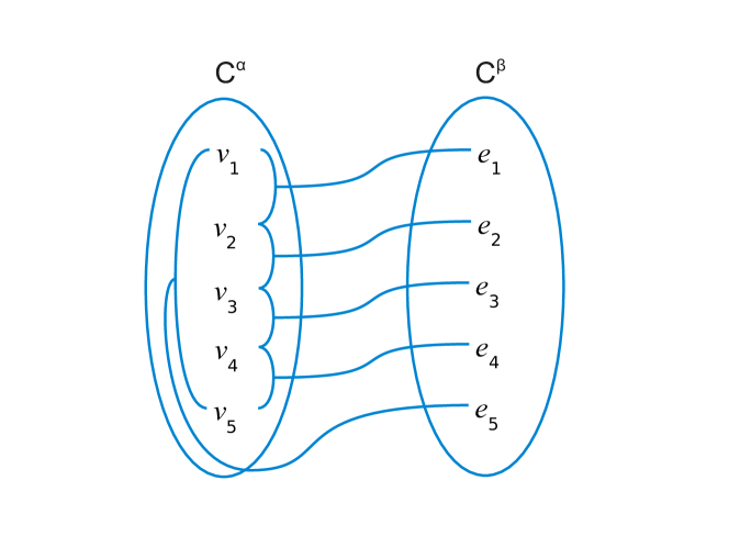
Figure 1: CSP encoding of the CGP on the graph $C_{5}$.

3 Structural Restrictions

In recent years, there has been a flurry of research into identifying tractable classes of classic CSP instances based on restrictions on the hypergraphs of CSP instances, known as structural restrictions. Below, we present and discuss a few representative examples. To present the various structural restrictions, we will use the framework of width functions, introduced by Adler [1].

Definition 6 (Hypergraph)

A hypergraph $\langle V,H\rangle$ is a set of vertices $V$ together with a set of hyperedges $H\subseteq\mathcal{P}(V)$.

Given a CSP instance $P=\langle V,C\rangle$, the hypergraph of $P$, denoted $\mathsf{hyp}(P)$, has vertex set $V$ together with a hyperedge $\mathcal{V}(\delta)$ for every $e[\delta]\in C$.

Definition 7 (Tree decomposition)

A tree decomposition of a hypergraph $\langle V,H\rangle$ is a pair $\langle T,\lambda\rangle$ where $T$ is a tree and $\lambda$ is a labelling function from nodes of $T$ to subsets of $V$, such that

1. for every $v\in V$, there exists a node $t$ of $T$ such that $v\in\lambda(t)$,

2. for every hyperedge $h\in H$, there exists a node $t$ of $T$ such that $h\subseteq\lambda(t)$, and

3. for every $v\in V$, the set of nodes $\{t\mid v\in\lambda(t)\}$ induces a connected subtree of $T$.

Definition 8 (Width function)

Let $G=\langle V,H\rangle$ be a hypergraph. A width function on $G$ is a function $f:\mathcal{P}(V)\rightarrow\mathbb{R}^{+}$ that assigns a positive real number to every nonempty subset of vertices of $G$. A width function $f$ is monotone if $f(X)\leq f(Y)$ whenever $X\subseteq Y$.

Let $\langle T,\lambda\rangle$ be a tree decomposition of $G$, and $f$ a width function on $G$. The $f$-width of $\langle T,\lambda\rangle$ is $\max(\{f(\lambda(t))\mid t\mbox{ node of }T\})$. The $f$-width of $G$ is the minimal $f$-width over all its tree decompositions.

In other words, a width function on a hypergraph $G$ tells us how to assign weights to nodes of tree decompositions of $G$.

Definition 9 (Treewidth)

Let $f(X)=|X|-1$. The treewidth $\mathsf{tw}(G)$ of a hypergraph $G$ is the $f$-width of $G$.

Let $G=\langle V,H\rangle$ be a hypergraph, and $X\subseteq V$. An edge cover for $X$ is any set of hyperedges $H^{\prime}\subseteq H$ that satisfies $X\subseteq\bigcup H^{\prime}$. The edge cover number $\rho(X)$ of $X$ is the size of the smallest edge cover for $X$. It is clear that $\rho$ is a width function.

Definition 10 ([1, Chapter 2])

The generalized hypertree width $\mathsf{hw}(G)$ of a hypergraph $G$ is the $\rho$-width of $G$.

Next, we define a relaxation of hypertree width known as fractional hypertree width, introduced by Grohe and Marx [20].

Definition 11 (Fractional edge cover)

Let $G=\langle V,H\rangle$ be a hypergraph, and $X\subseteq V$. A fractional edge cover for $X$ is a function $\gamma:H\rightarrow[0,1]$ such that $\displaystyle\sum_{v\in h\in H}\gamma(h)\geq 1$ for every $v\in X$. We call $\displaystyle\sum_{h\in H}\gamma(h)$ the weight of $\gamma$. The fractional edge cover number $\rho^{*}(X)$ of $X$ is the minimum weight over all fractional edge covers for $X$. It is known that this minimum is always rational [20].

Definition 12

The fractional hypertree width $\mathsf{fhw}(G)$ of a hypergraph $G$ is the $\rho^{*}$-width of $G$.

For a class of hypergraphs $\mathcal{H}$ and a notion of width $\alpha$, we write $\alpha(\mathcal{H})$ for the maximal $\alpha$-width over the hypergraphs in $\mathcal{H}$. If this is unbounded we write $\alpha(\mathcal{H})=\infty$; otherwise $\alpha(\mathcal{H})<\infty$.

All the above restrictions can be used to guarantee tractability for classes of CSP instances where all constraints are table constraints.

Theorem 3.1 ([10, 17, 20])

Let $\mathcal{H}$ be a class of hypergraphs. For every $\alpha\in\{\mathsf{hw},\mathsf{fhw}\}$, any class of classic CSP instances whose hypergraphs are in $\mathcal{H}$ is tractable if $\alpha(\mathcal{H})<\infty$.

To go beyond fractional hypertree width, Marx [25, 24] recently introduced the concept of submodular width. This concept uses a set of width functions satisfying a condition (submodularity), and considers the $f$-width of a hypergraph for every such function $f$.

Definition 13 (Submodular width function)

Let $G=\langle V,H\rangle$ be a hypergraph. A width function $f$ on $G$ is submodular if for every set $X,Y\subseteq V$, we have $f(X)+f(Y)\geq f(X\cap Y)+f(X\cup Y)$.

Definition 14 (Submodular width)

Let $G$ be a hypergraph. The submodular width $\mathsf{subw}(G)$ of $G$ is the maximum $f$-width of $G$ taken over all monotone submodular width functions $f$ on $G$.

For a class of hypergraphs $\mathcal{H}$, we write $\mathsf{subw}(\mathcal{H})$ for the maximal submodular width over the hypergraphs in $\mathcal{H}$. If this is unbounded we write $\mathsf{subw}(\mathcal{H})=\infty$; otherwise $\mathsf{subw}(\mathcal{H})<\infty$.

Unlike for fractional hypertree width and every other structural restriction discussed so far, the running time of the algorithm given by Marx for classic CSP instances with bounded submodular width has an exponential dependence on the number of vertices in the hypergraph of the instance. The class of classic CSP instances with bounded submodular width is therefore not tractable. However, this class is what is called fixed-parameter tractable [11, 12].

Definition 15 (Fixed-parameter tractable)

A parameterized problem instance is a pair $\langle k,P\rangle$, where $P$ is a problem instance, such as a CSP instance, and $k\in\mathbb{N}$ a parameter.

Let $S$ be a class of parameterized problem instances. We say that $S$ is fixed-parameter tractable (in ) if there is a function $f$ of one argument, as well as a constant $c$, such that every problem $\langle k,P\rangle\in S$ can be solved in time $O(f(k)\times|P|^{c})$.

The function $f$ can be arbitrary, but must only depend on the parameter $k$. For CSP instances, a natural parameterization is by the size of the hypergraph of an instance, measured by the number of vertices. Since the hypergraph of an instance has a vertex for every variable, for every CSP instance $P=\langle V,C\rangle$ we consider the parameterized instance $\langle|V|,P\rangle$.

Theorem 3.2 ([24])

Let $\mathcal{H}$ be a class of hypergraphs. If $\mathsf{subw}(\mathcal{H})<\infty$, then a class of classic CSP instances whose hypergraphs are in $\mathcal{H}$ is in .

The three structural restrictions that we have just presented form a hierarchy [20, 24]: For every hypergraph $G$, $\mathsf{subw}(G)\leq\mathsf{fhw}(G)\leq\mathsf{hw}(G)$.

As the example below demonstrates, Theorem 3.1 does not hold for CSP instances with arbitrary global constraints, even if we have a fixed, finite domain.

Example 4

The -complete problem of 3-colourability [13] is to decide, given a graph $\langle V,E\rangle$, whether the vertices $V$ can be coloured with three colours such that no two adjacent vertices have the same colour.

We may reduce this problem to a CSP with EGC constraints (cf. Example 1) as follows: Let $V$ be the set of variables for our CSP instance, each with domain $\{r,g,b\}$. For every edge $\langle v,w\rangle\in E$, we post an EGC constraint with scope $\{v,w\}$, parameterized by the function $K$ such that $K(r)=K(g)=K(b)=\{0,1\}$. Finally, we make the hypergraph of this CSP instance have low width by adding an EGC constraint with scope $V$ parameterized by the function $K^{\prime}$ such that $K^{\prime}(r)=K^{\prime}(g)=K^{\prime}(b)=\{0,\ldots,|V|\}$. This reduction clearly takes polynomial time, and the hypergraph $G$ of the resulting instance has $\mathsf{hw}(G)=\mathsf{fhw}(G)=\mathsf{subw}(G)=1$.

As the constraint with scope $V$ allows all possible assignments, any solution to this CSP is also a solution to the 3-colourability problem, and vice versa.

Likewise, Theorem 3.2 does not hold for CSP instances with arbitrary global constraints if we allow the variables unbounded domain size, that is, change the above example to $k$-colourability. With that in mind, in the rest of the paper we will identify properties of extensionally represented constraints that these structural restrictions exploit to guarantee tractability. Then, we are going to look for restricted classes of global constraints that possess these properties. To do so, we will use the following definitions.

Definition 16 (Constraint catalogue)

A constraint catalogue is a set of global constraints. A CSP instance $\langle V,C\rangle$ is said to be over a constraint catalogue $\Gamma$ if for every $e[\delta]\in C$ we have $e[\delta]\in\Gamma$.

Definition 17 (Restricted CSP class)

Let $\Gamma$ be a constraint catalogue, and let $\mathcal{H}$ be a class of hypergraphs. We define $\textup{CSP}(\mathcal{H},\Gamma)$ to be the class of CSP instances over $\Gamma$ whose hypergraphs are in $\mathcal{H}$.

Definition 17 allows us to discuss classic CSP instances alongside instances with global constraints. Let $\mathbf{Ext}$ be the constraint catalogue containing all table global constraints. The classic CSP instances are then precisely those that are over $\mathbf{Ext}$. In particular, we can now restate Theorems 3.1 and 3.2 as follows.

Theorem 3.3

Let $\mathcal{H}$ be a class of hypergraphs. For every $\alpha\in\{\mathsf{hw},\mathsf{fhw}\}$, the class of CSP instances $\textup{CSP}(\mathcal{H},\mathbf{Ext})$ is tractable if $\alpha(\mathcal{H})<\infty$. Furthermore, if $\mathsf{subw}(\mathcal{H})<\infty$ then $\textup{CSP}(\mathcal{H},\mathbf{Ext})$ is in .

4 Properties of Extensional Representation

We are going to start our investigation by considering fractional hypertree width in more detail. To obtain tractability for classic CSP instances of bounded fractional hypertree width, Grohe and Marx [20] use a bound on the number of solutions to a classic CSP instance, and show that this bound is preserved when we consider parts of a CSP instance. The following definition formalizes what we mean by “parts”, and is required to state the algorithm that Grohe and Marx use in their paper.

Definition 18 (Constraint projection)

Let $e[\delta]$ be a constraint. The projection of $e[\delta]$ onto a set of variables $X\subseteq\mathcal{V}(\delta)$ is the constraint $\mathsf{pj}_{X}(e[\delta])$ such that $\mu\in\mathsf{pj}_{X}(e[\delta])$ if and only if there exists $\theta\in e[\delta]$ with $\theta|_{X}=\mu$.

For a CSP instance $P=\langle V,C\rangle$ and $X\subseteq V$ we define $\mathsf{pj}_{X}(P)=\langle X,C^{\prime}\rangle$, where $C^{\prime}$ is the least set containing for every $e[\delta]\in C$ such that $X\cap\mathcal{V}(\delta)\not=\emptyset$ the constraint $\mathsf{pj}_{X\cap\mathcal{V}(\delta)}(e[\delta])$.

Their algorithm is given as Algorithm 1, and is essentially the usual recursive search algorithm for finding all solutions to a CSP instance by considering smaller and smaller sub-instances using constraint projections.

procedure EnumSolutions(CSP instance $P=\langle V,C\rangle$)$\triangleright$ Returns $\mathsf{sol}(P)$

     $\textup{Solutions}\leftarrow\emptyset$

     if $V=\emptyset$ then

         return $\{\bot\}$$\triangleright$ The empty assignment

     else

         $w\leftarrow\textup{chooseVar}(V)$$\triangleright$ Pick a variable from $V$

         $\Theta=\textup{EnumSolutions}(\mathsf{pj}_{V-\{w\}}(P))$

         for $\theta\in\Theta$ do

              for $a\in D(w)$ do

                  if $\theta\cup\langle w,a\rangle$ is a solution to $P$ then

                       $\textup{Solutions.add}(\theta\cup\langle w,a\rangle)$

                  end if

              end for

         end for

     end if

     return Solutions

end procedure

Algorithm 1 Enumerate all solutions of a CSP instance

To show that Algorithm 1 does indeed find all solutions, we will use the following property of constraint projections.

Lemma 1

Let $P=\langle V,C\rangle$ be a CSP instance. For every $X\subseteq V$, we have $\mathsf{sol}(\mathsf{pj}_{X}(P))\supseteq\pi_{X}(\mathsf{sol}(P))$.

Proof

Given $P=\langle V,C\rangle$, let $X\subseteq V$ be arbitrary, and let $C^{\prime}=\{e[\delta]\in C\mid X\cap\mathcal{V}(\delta)\not=\emptyset\}$. For every $\theta\in\mathsf{sol}(P)$ and constraint $e[\delta]\in C^{\prime}$ we have that $\theta|_{\mathcal{V}(\delta)}\in e[\delta]$ since $\theta$ is a solution to $P$. By Definition 18, it follows that for every $e[\delta]\in C^{\prime}$, $\theta|_{X\cap\mathcal{V}(\delta)}\in\mathsf{pj}_{X\cap\mathcal{V}(\delta)}(e[\delta])$. Since the set of constraints of $\mathsf{pj}_{X}(P)$ is the least set containing for each $e[\delta]\in C^{\prime}$ the constraint $\mathsf{pj}_{X\cap\mathcal{V}(\delta)}(e[\delta])$, we have $\theta|_{X}\in\mathsf{sol}(\mathsf{pj}_{X}(P))$, and hence $\mathsf{sol}(\mathsf{pj}_{X}(P))\supseteq\pi_{X}(\mathsf{sol}(P))$. Since $X$ was arbitrary, the claim follows.

Theorem 4.1 (Correctness of Algorithm 1)

Let $P$ be a CSP instance. We have that $\textup{EnumSolutions}(P)=\mathsf{sol}(P)$.

Proof

The proof is by induction on the set of variables $V$ in $P$. For the base case, if $V=\emptyset$, the empty assignment is the only solution.

Otherwise, choose a variable $w\in V$, and let $X=V-\{w\}$. By induction, we can assume that $\textup{EnumSolutions}(\mathsf{pj}_{X}(P))=\mathsf{sol}(\mathsf{pj}_{X}(P))$. Since for every $\theta\in\mathsf{sol}(P)$ there exists $a\in D(w)$ such that $\theta=\theta|_{X}\cup\langle w,a\rangle$, and furthermore $\theta|_{X}\in\pi_{X}(\mathsf{sol}(P))$, it follows by Lemma 1 that $\theta|_{X}\in\mathsf{sol}(\mathsf{pj}_{X}(P))$. Since Algorithm 1 checks every assignment of the form $\mu\cup\langle w,a\rangle$ for every $\mu\in\mathsf{sol}(\mathsf{pj}_{X}(P))$ and $a\in D(w)$, it follows that $\textup{EnumSolutions}(P)=\mathsf{sol}(P)$.

The time required for this algorithm depends on three key factors, which we are going to enumerate and discuss below. Let

1. $s(P)$ be the maximum of the number of solutions to each of the instances $\mathsf{pj}_{V-\{w\}}(P)$,

2. $c(P)$ be the maximum time required to check whether an assignment is a solution to $P$, and

3. $b(P)$ be the maximum time required to construct any instance $\mathsf{pj}_{V-\{w\}}(P)$.

There are $|V|$ calls to EnumSolutions. For each call, we need $b(P)$ time to construct the projection, while the double loop takes at most $s(P)\times|D(w)|\times c(P)$ time. Therefore, letting $d=\max(\{|D(w)|\mid w\in V\})$, the running time of Algorithm 1 is bounded by $O\big{(}|V|\times(s(P)\times d\times c(P)+b(P))\big{)}$.

Since constructing the projection of a classic CSP instance can be done in polynomial time, and likewise checking that an assignment is a solution, the whole algorithm runs in polynomial time if $s(P)$ is a polynomial in the size of $P$. For fractional hypertree width, Grohe and Marx show the following.

Lemma 2 ([20])

A classic CSP instance $P$ has at most $|P|^{\mathsf{fhw}(\mathsf{hyp}(P))}$ solutions.

Since fractional hypertree width is a monotone width function, it follows that for any instance $P=\langle V,C\rangle$ and $X\subseteq V$, $\mathsf{fhw}(\mathsf{hyp}(\mathsf{pj}_{X}(P)))\leq\mathsf{fhw}(\mathsf{hyp}(P))$. Therefore, for classic CSP instances of bounded fractional hypertree width $s(P)$ is indeed polynomial in $|P|$.

5 CSP Instances with Few Solutions in Key Places

Having few solutions for every projection of a CSP instance is thus a property that makes fractional hypertree width yield tractable classes of classic CSP instances. More importantly, we have shown that this property allows us to find all solutions to a CSP instance $P$, even with global constraints, if we can build arbitrary projections of $P$ in polynomial time. In other words, with these two conditions we should be able to reduce instances with global constraints to classic instances in polynomial time.

However, on reflection there is no reason why we should need few solutions for every projection. Instead, consider the following reduction.

Definition 19 (Partial assignment checking)

A global constraint catalogue $\Gamma$ allows partial assignment checking if for any constraint $e[\delta]\in\Gamma$ we can decide in polynomial time whether a given assignment $\theta$ to a set of variables $W\subseteq\mathcal{V}(\delta)$ is contained in an assignment that satisfies $e[\delta]$, i.e. whether there exists $\mu\in e[\delta]$ such that $\theta=\mu|_{W}$.

As an example, a catalogue that contains arbitrary EGC constraints (cf. Example 1) does not satisfy Definition 19, since checking whether an arbitrary EGC constraint has a satisfying assignment is -hard [26]. On the other hand, a catalogue that contains only EGC constraints whose cardinality sets are intervals does satisfy Definition 19 [27].

If a catalogue $\Gamma$ satisfies Definition 19, we can for any constraint $e[\delta]\in\Gamma$ build arbitrary projections of it, that is, construct the global constraint $\mathsf{pj}_{X}(e[\delta])$ for any $X\subseteq\mathcal{V}(\delta)$, in polynomial time.

Definition 20 (Intersection variables)

Let $\langle V,C\rangle$ be a CSP instance. The set of intersection variables of any constraint $e[\delta]\in P$ is $\mathsf{iv}(\delta)=\bigcup\{\mathcal{V}(\delta)\cap\mathcal{V}(\delta^{\prime})\mid e^{\prime}[\delta^{\prime}]\in C-\{e[\delta]\}\}$.

Definition 21 (Table constraint induced by a global constraint)

Let $P=\langle V,C\rangle$ be a CSP instance. For every $e[\delta]\in C$, let $\mu^{*}$ be the assignment to $\mathcal{V}(\delta)-\mathsf{iv}(\delta)$ that assigns a special value $*$ to every variable. The table constraint induced by $e[\delta]$ is $\mathsf{ic}(e[\delta])=e^{\prime}[\delta^{\prime}]$, where $\mathcal{V}(\delta^{\prime})=\mathcal{V}(\delta)$, and $\delta^{\prime}$ contains for every assignment $\theta\in\mathsf{sol}(\mathsf{pj}_{\mathsf{iv}(\delta)}(P))$ the assignment $\theta\oplus\mu^{*}$.

If every constraint in a CSP instance $P=\langle V,C\rangle$ allows partial assignment checking, then building $\mathsf{ic}(e[\delta])$ for any $e[\delta]\in C$ can be done in polynomial time when $|\mathsf{sol}(\mathsf{pj}_{X}(P))|$ is itself polynomial in the size of $P$ for every subset $X$ of $\mathsf{iv}(\delta)$. To do so, we can invoke Algorithm 1 on the instance $\mathsf{pj}_{\mathsf{iv}(\delta)}(P)$. The definition below expresses this idea.

Definition 22 (Sparse intersections)

A class of CSP instances $\mathcal{P}$ has sparse intersections if there exists a constant $c$ such that for every constraint $e[\delta]$ in any instance $P\in\mathcal{P}$, we have that for every $X\subseteq\mathsf{iv}(\delta)$, $|\mathsf{sol}(\mathsf{pj}_{X}(P))|\leq|P|^{c}$.

If a class of instances $\mathcal{P}$ has sparse intersections, and the instances are all over a constraint catalogue that allows partial assignment checking, then we can for every constraint $e[\delta]$ of any instance from $\mathcal{P}$ construct $\mathsf{ic}(e[\delta])$ in polynomial time. While this definition considers the instance as a whole, one special case of it is the case where every constraint has few solutions in the size of its description, that is, there is a constant $c$ and the constraints are drawn from a catalogue $\Gamma$ such that for every $e[\delta]\in\Gamma$, we have that $|\{\mu\mid\mu\in e[\delta]\}|\leq|\delta|^{c}$.

Theorem 5.1

Let $\mathcal{P}$ be a class of CSP instances over a catalogue that allows partial assignment checking. If $\mathcal{P}$ has sparse intersections, then we can in polynomial time reduce any instance $P\in\mathcal{P}$ to a classic CSP instance $P_{CL}$ with $\mathsf{hyp}(P)=\mathsf{hyp}(P_{CL})$, such that $P_{CL}$ has a solution if and only if $P$ does.

Proof

Let $P=\langle V,C\rangle$ be an instance from such a class $\mathcal{P}$. For each $e[\delta]\in C$, $P_{CL}$ will contain the table constraint $\mathsf{ic}(e[\delta])$ from Definition 21. Since $P$ is over a catalogue that allows partial assignment checking, and $\mathcal{P}$ has sparse intersections, computing $\mathsf{ic}(e[\delta])$ can be done in polynomial time by invoking Algorithm 1 on $\mathsf{pj}_{\mathsf{iv}(\delta)}(P)$.

It is clear that $\mathsf{hyp}(P)=\mathsf{hyp}(P_{CL})$. All that is left to show is that $P_{CL}$ has a solution if and only if $P$ does. Let $\theta$ be a solution to $P=\langle V,C\rangle$. For every $e[\delta]\in C$, we have that $\theta|_{\mathsf{iv}(\delta)}\in\mathsf{pj}_{\mathsf{iv}(\delta)}(P)$ by Definitions 18 and 20, and the assignment $\mu$ that assigns the value $\theta(v)$ to each $v\in\displaystyle\bigcup_{e[\delta]\in C}\mathsf{iv}(\delta)$, and $*$ to every other variable is therefore a solution to $P_{CL}$.

In the other direction, if $\theta$ is a solution to $P_{CL}$, then $\theta$ satisfies $\mathsf{ic}(e[\delta])$ for every $e[\delta]\in C$. By Definition 21, this means that $\theta|_{\mathsf{iv}(\delta)}\in\mathsf{sol}(\mathsf{pj}_{\mathsf{iv}(\delta)}(P))$, and by Definition 18, there exists an assignment $\mu^{e[\delta]}$ with $\mu^{e[\delta]}|_{\mathsf{iv}(\delta)}=\theta|_{\mathsf{iv}(\delta)}$ that satisfies $e[\delta]$. By Definition 20, the variables not in $\mathsf{iv}(\delta)$ do not occur in any other constraint in $P$, so we can combine all the assignments $\mu^{e[\delta]}$ to form a solution $\mu$ to $P$ such that for $e[\delta]\in C$ and $v\in\mathcal{V}(\delta)$ we have $\mu(v)=\mu^{e[\delta]}(v)$.

From Theorem 5.1, we get tractable and fixed-parameter tractable classes of CSP instances with global constraints.

Corollary 1

Let $\mathcal{H}$ be a class of hypergraphs, and $\Gamma$ a catalogue that allows partial assignment checking. If $\textup{CSP}(\mathcal{H},\Gamma)$ has sparse intersections, then $\textup{CSP}(\mathcal{H},\Gamma)$ is tractable or in if $\textup{CSP}(\mathcal{H},\mathbf{Ext})$ is.

Proof

Let $\mathcal{H}$ and $\Gamma$ be given. By Theorem 5.1, we can reduce any $P\in\textup{CSP}(\mathcal{H},\Gamma)$ to an instance $P_{CL}\in\textup{CSP}(\mathcal{H},\mathbf{Ext})$ in polynomial time. Since $P_{CL}$ has a solution if and only if $P$ does, tractability or fixed-parameter tractability of $\textup{CSP}(\mathcal{H},\mathbf{Ext})$ implies the same for $\textup{CSP}(\mathcal{H},\Gamma)$.

5.1 Applying Corollary 1 to the CGP

Recall the connected graph partition problem (Problem 1): Given a connected graph $G$, as well as natural numbers $\alpha$ and $\beta$, can the vertices of $G$ be partitioned into bags of size at most $\alpha$, such that no more than $\beta$ edges are broken. Using the CSP encoding we gave in Example 3, as well as Corollary 1, we will show a new result, that this problem is tractable if $\beta$ is fixed. To simplify the analysis, we assume without loss of generality that $\alpha<|V|$, which means that any solution has at least one broken edge.

We claim that if $\beta$ is fixed, then the constraint $C^{\beta}=e^{\beta}[\delta^{\beta}]$ allows partial assignment checking, and has only a polynomial number of satisfying assignments. The latter implies that for any instance $P$ of the CGP, $|\mathsf{sol}(\mathsf{pj}_{\mathsf{iv}(\delta^{\beta})}(P))|$ is polynomial in the size of $P$ for every subset of $\mathsf{iv}(\delta^{\beta})$. Furthermore, we will show that for the constraint $C^{\alpha}=e^{\alpha}[\delta^{\alpha}]$, we also have that $|\mathsf{sol}(\mathsf{pj}_{\mathsf{iv}(\delta^{\alpha})}(P))|$ is polynomial in the size of $P$. That $C^{\alpha}$ allows partial assignment checking follows from a result by Régin [27], since the cardinality sets of $C^{\alpha}$ are intervals.

First, we show that the number of satisfying assignments to $C^{\beta}$ is limited. Since $C^{\beta}$ limits the number of ones in any solution to $\beta$ or fewer, the number of satisfying assignments to this constraint is the number of ways to choose up to $\beta$ variables to be assigned one. This is bounded by $\displaystyle\sum^{\beta}_{i=1}\binom{|E|}{i}\leq(|E|+1)^{\beta}$, and so we can generate them all in polynomial time.

Now, let $\theta$ be such a solution. How many solutions to $P$ contain $\theta$? Well, every constraint on $\{u,v,e\}$ with $e=1$ allows at most $|V|^{2}$ assignments, and there are at most $\beta$ such constraints. So far we therefore have at most $(|E|+1)^{\beta}\times|V|^{2\beta}$ assignments.

On the other hand, a ternary constraint with $e=0$ requires $u=v$. Consider the graph $G_{0}$ containing for every constraint on $\{u,v,e\}$ with $e=0$ the vertices $u$ and $v$ as well as the edge $\{u,v\}$. Since the original graph was connected, every connected component of $G_{0}$ contains at least one vertex which is in the scope of some constraint with $e=1$. Therefore, since equality is transitive, each connected component of $G_{0}$ allows at most one assignment for each of the $(|E|+1)^{\beta}\times|V|^{2\beta}$ assignments to the other variables of $P$. We therefore get a total bound of $(|E|+1)^{\beta}\times|V|^{2\beta}$ on the total number of solutions to $P$, and hence to $\mathsf{pj}_{\mathsf{iv}(\delta^{\alpha})}(P)$.

The hypergraph of any CSP instance $P$ encoding the CGP has two hyperedges covering the whole problem, so the hypertree width of this hypergraph is two. Therefore, we may apply Corollaries 1 and 3.1 to obtain tractability when $\beta$ is fixed. As this problem is -complete for fixed $\alpha\geq 3$ [13, p. 209], $\beta$ is a natural parameter to try and use.

As it happens, in this problem we can drop the requirement of partial assignment checking for the constraint $C^{\alpha}$. All its variables are intersection variables, and the instance has few solutions even if we disregard $C^{\alpha}$. Thus, we need only check whether any of those solutions satisfy $C^{\alpha}$, and checking whether an assignment to the whole scope of a constraint satisfies it can always be done in polynomial time by Definition 4. In the next section, we turn this observation into a general result.

6 Back Doors

If a class of CSP instances includes constraints from a catalogue that is not known to allow partial assignment checking, we may still obtain tractability in some cases by applying the notion of a back door set. A (strong) back door set [14, 32] is a set of variables in a CSP instance that, when assigned, make the instance easy to solve. Below, we are going to adapt this notion to individual constraints.

Definition 23 (Back door)

Let $\Gamma$ be a global constraint catalogue. A back door for a constraint $e[\delta]\in\Gamma$ is any set of variables $W\subseteq\mathcal{V}(\delta)$ (called a back door set) such that we can decide in polynomial time whether a given assignment $\theta$ to a set of variables $\mathcal{V}(\theta)\supseteq W$ is contained in an assignment that satisfies $e[\delta]$, i.e. whether there exists $\mu\in e[\delta]$ such that $\mu|_{\mathcal{V}(\theta)}=\theta$.

Trivially, for every constraint $e[\delta]$ the set of variables $\mathcal{V}(\delta)$ is a back door set, since by Definition 4 we can always check in polynomial time if an assignment to $\mathcal{V}(\delta)$ satisfies the constraint $e[\delta]$.

The key point about back doors is that given a catalogue $\Gamma$, adding to each $e[\delta]\in\Gamma$ with back door set $W$ an arbitrary set of assignments to $W$ produces a catalogue $\Gamma^{\prime}$ that allows partial assignment checking. Adding a set of assignments $\Theta$ means to add $\Theta$ to the description, and modify the algorithm $e$ to only accept an assignment if it contains a member of $\Theta$ in addition to previous requirements. Furthermore, given a CSP instance $P$ containing $e[\delta]$, as long as $\Theta\supseteq\pi_{W}(\mathsf{sol}(P))$, adding $\Theta$ to $e[\delta]$ produces an instance that has exactly the same solutions. This point leads to the following definition.

Definition 24 (Sparse back door cover)

Let $\Gamma_{PAC}$ be a catalogue that allows partial assignment checking and $\Gamma_{BD}$ a catalogue. For every instance $P=\langle V,C\rangle$ over $\Gamma_{PAC}\cup\Gamma_{BD}$, let $P\cap\Gamma_{PAC}$ be the instance with constraint set $C^{\prime}=C\cap\Gamma_{PAC}$ and set of variables $\bigcup\{V\cap\mathcal{V}(\delta)\mid e[\delta]\in C^{\prime}\}$.

A class of CSP instances $\mathcal{P}$ over $\Gamma_{PAC}\cup\Gamma_{BD}$ has sparse back door cover if there exists a constant $c$ such that for every instance $P=\langle V,C\rangle\in\mathcal{P}$ and constraint $e[\delta]\in C$, if $e[\delta]\not\in\Gamma_{PAC}$, then there exists a back door set $W$ for $e[\delta]$ with $|\mathsf{sol}(\mathsf{pj}_{X}(P\cap\Gamma_{PAC}))|\leq|P|^{c}$ for every $X\subseteq W$.

Sparse back door cover means that for each constraint that is not from a catalogue that allows partial assignment checking, we can in polynomial time get a set of assignments $\Theta$ for its back door set using Algorithm 1, and so turn this constraint into one that does allow partial assignment checking. This operation preserves the solutions of the instance that contains this constraint.

Theorem 6.1

If a class of CSP instance $\mathcal{P}$ has sparse back door cover, then we can in polynomial time reduce any instance $P\in\mathcal{P}$ to an instance $P^{\prime}$ such that $\mathsf{hyp}(P)=\mathsf{hyp}(P^{\prime})$ and $\mathsf{sol}(P)=\mathsf{sol}(P^{\prime})$. Furthermore, the class of instances $\{P^{\prime}\mid P\in\mathcal{P}\}$ is over a catalogue that allows partial assignment checking.

Proof

Let $P=\langle V,C\rangle\in\mathcal{P}$. We construct $P^{\prime}$ by adding to every $e[\delta]\in C$ such that $e[\delta]\not\in\Gamma_{PAC}$, with back door set $W$, the set of assignments $\mathsf{sol}(\mathsf{pj}_{W}(P\cap\Gamma_{PAC}))$, which we can obtain using Algorithm 1. By Definition 24, we have for every $X\subseteq W$ that $|\mathsf{sol}(\mathsf{pj}_{W}(P\cap\Gamma_{PAC}))|\leq|P|^{c}$, so Algorithm 1 takes polynomial time since $\Gamma_{PAC}$ does allow partial assignment checking.

It is clear that $\mathsf{hyp}(P^{\prime})=\mathsf{hyp}(P)$, and since $\mathsf{sol}(\mathsf{pj}_{W}(P\cap\Gamma_{PAC}))\supseteq\pi_{W}(\mathsf{sol}(P))$, the set of solutions stays the same, i.e. $\mathsf{sol}(P^{\prime})=\mathsf{sol}(P)$. Finally, since we have replaced each constraint $e[\delta]$ in $P$ that was not in $\Gamma_{PAC}$ by a constraint that does allow partial assignment checking, it follows that $P^{\prime}$ is over a catalogue that allows partial assignment checking.

One consequence of Theorem 6.1 is that we can sometimes apply Theorem 5.1 to a CSP instance that contains a constraint for which checking if a partial assignment can be extended to a satisfying one is hard. We can do so when the variables of that constraint are covered by the variables of other constraints that do allow partial assignment checking — but only if the instance given by those constraints has few solutions.

As a concrete example of this, consider again the encoding of the CGP that we gave in Example 3. The variables of constraint $C^{\alpha}$ are entirely covered by the instance $P^{\prime}$ obtained by removing $C^{\alpha}$. As the entire set of variables of a constraint is a back door set for it, and the instance $P^{\prime}$ has few solutions (cf. Section 5.1), this class of instances has sparse back door cover. As such, the constraint $C^{\alpha}$ could, in fact, be arbitrary without affecting the tractability of this problem. In particular, the requirement that $C^{\alpha}$ allows partial assignment checking can be dropped.

7 Summary and Future Work

In this paper, we have investigated properties that many structural restrictions rely on to yield tractable classes of CSP instances with explicitly represented constraints. In particular, we identify a relationship between the number of solutions and the size of a CSP instance as being one such property. Using this insight, we show that known structural restrictions yield tractability for any class of CSP instances with global constraints that satisfies this property. In particular, the above implies that the structural restrictions we consider yield tractability for classes of instances where every global constraint has few satisfying assignments relative to its size.

To illustrate our result, we apply it to a known problem, the connected graph partition problem, and use it to identify a new tractable case of this problem. We also demonstrate how the concept of back doors, subsets of variables that make a problem easy to solve once assigned, can be used to relax the conditions of our result in some cases.

As for future work, one obvious research direction to pursue is to find a complete characterization of tractable classes of CSP instances with sparse intersections. Another avenue of research would be to apply the results in this paper to various kinds of valued CSP.

References

- [1] Adler, I.: Width Functions for Hypertree Decompositions. Doctoral dissertation, Albert-Ludwigs-Universität Freiburg (2006)
- [2] Aschinger, M., Drescher, C., Friedrich, G., Gottlob, G., Jeavons, P., Ryabokon, A., Thorstensen, E.: Optimization methods for the partner units problem. In: Proc. CPAIOR’11. LNCS, vol. 6697, pp. 4–19. Springer (2011)
- [3] Aschinger, M., Drescher, C., Gottlob, G., Jeavons, P., Thorstensen, E.: Structural decomposition methods and what they are good for. In: Schwentick, T., Dürr, C. (eds.) Proc. STACS’11. LIPIcs, vol. 9, pp. 12–28 (2011)
- [4] Bessiere, C., Hebrard, E., Hnich, B., Walsh, T.: The complexity of reasoning with global constraints. Constraints 12(2), 239–259 (2007)
- [5] Bessiere, C., Katsirelos, G., Narodytska, N., Quimper, C.G., Walsh, T.: Decomposition of the NValue constraint. In: Proc. CP’10. LNCS, vol. 6308, pp. 114–128. Springer (2010)
- [6] Bulatov, A., Jeavons, P., Krokhin, A.: Classifying the complexity of constraints using finite algebras. SIAM Journal on Computing 34(3), 720–742 (2005)
- [7] Chen, H., Grohe, M.: Constraint satisfaction with succinctly specified relations. Journal of Computer and System Sciences 76(8), 847–860 (2010)
- [8] Cohen, D., Jeavons, P., Gyssens, M.: A unified theory of structural tractability for constraint satisfaction problems. Journal of Computer and System Sciences 74(5), 721–743 (2008)
- [9] Cohen, D.A., Green, M.J., Houghton, C.: Constraint representations and structural tractability. In: Proc. CP’09. LNCS, vol. 5732, pp. 289–303. Springer (2009)
- [10] Dalmau, V., Kolaitis, P.G., Vardi, M.Y.: Constraint satisfaction, bounded treewidth, and finite-variable logics. In: Proc. CP’02. LNCS, vol. 2470, pp. 223–254. Springer (2002)
- [11] Downey, R.G., Fellows, M.R.: Parameterized Complexity. Monographs in Computer Science, Springer (1999)
- [12] Flum, J., Grohe, M.: Parameterized Complexity Theory. Texts in Theoretical Computer Science, Springer (2006)
- [13] Garey, M.R., Johnson, D.S.: Computers and Intractability: A Guide to the Theory of NP-Completeness. W. H. Freeman (1979)
- [14] Gaspers, S., Szeider, S.: Backdoors to satisfaction. In: Bodlaender, H.L., Downey, R., Fomin, F.V., Marx, D. (eds.) The Multivariate Algorithmic Revolution and Beyond, LNCS, vol. 7370, pp. 287–317. Springer (2012)
- [15] Gent, I.P., Jefferson, C., Miguel, I.: MINION: A fast, scalable constraint solver. In: Proc. ECAI’06, pp. 98–102. IOS Press (2006)
- [16] Gottlob, G., Leone, N., Scarcello, F.: A comparison of structural CSP decomposition methods. Artificial Intelligence 124(2), 243–282 (2000)
- [17] Gottlob, G., Leone, N., Scarcello, F.: Hypertree decompositions and tractable queries. Journal of Computer and System Sciences 64(3), 579–627 (2002)
- [18] Green, M.J., Jefferson, C.: Structural tractability of propagated constraints. In: Proc. CP’08. LNCS, vol. 5202, pp. 372–386. Springer (2008)
- [19] Grohe, M.: The complexity of homomorphism and constraint satisfaction problems seen from the other side. Journal of the ACM 54(1), 1–24 (2007)
- [20] Grohe, M., Marx, D.: Constraint solving via fractional edge covers. In: Proc. SODA’06, pp. 289–298. ACM (2006)
- [21] Hermenier, F., Demassey, S., Lorca, X.: Bin repacking scheduling in virtualized datacenters. In: Lee, J. (ed.) Proc. CP’11. LNCS, vol. 6876, pp. 27–41. Springer (2011)
- [22] van Hoeve, W.J., Katriel, I.: Global constraints. In: Rossi, F., van Beek, P., Walsh, T. (eds.) Handbook of Constraint Programming, Foundations of Artificial Intelligence, vol. 2, pp. 169–208. Elsevier (2006)
- [23] Kutz, M., Elbassioni, K., Katriel, I., Mahajan, M.: Simultaneous matchings: Hardness and approximation. Journal of Computer and System Sciences 74(5), 884–897 (August 2008)
- [24] Marx, D.: Tractable hypergraph properties for constraint satisfaction and conjunctive queries. CoRR abs/0911.0801 (2009)
- [25] Marx, D.: Tractable hypergraph properties for constraint satisfaction and conjunctive queries. In: Proc. STOC’10, pp. 735–744. ACM (2010)
- [26] Quimper, C.G., López-Ortiz, A., van Beek, P., Golynski, A.: Improved algorithms for the global cardinality constraint. In: Proc. CP’04. LNCS, vol. 3258, pp. 542–556. Springer (2004)
- [27] Régin, J.C.: Generalized Arc Consistency for Global Cardinality Constraint. In: Proc. AAAI’96, pp. 209–215. AAAI Press (1996)
- [28] Rossi, F., van Beek, P., Walsh, T. (eds.): The Handbook of Constraint Programming. Elsevier (2006)
- [29] Samer, M., Szeider, S.: Tractable cases of the extended global cardinality constraint. Constraints 16(1), 1–24 (2011)
- [30] Wallace, M.: Practical applications of constraint programming. Constraints 1, 139–168 (September 1996)
- [31] Wallace, M., Novello, S., Schimpf, J.: ECLiPSe: A platform for constraint logic programming. ICL Systems Journal 12(1), 137–158 (May 1997)
- [32] Williams, R., Gomes, C.P., Selman, B.: Backdoors to typical case complexity. In: Proc. IJCAI’03, pp. 1173–1178 (2003)