POPULATION OF ROTATIONAL STATES IN THE GROUND-BAND OF FISSION FRAGMENTS

Abstract

The population of rotational states in the ground-state band of neutron-rich fragments emitted in the spontaneous fission of ²⁵²Cf is described within a time-dependent quantum model similar to the one used for Coulomb excitation. The initial population probability of the states included in the selected basis is calculated according to the bending model at scission. Subsequently these initial amplitudes are feeding the coupled dynamical equations describing the population of rotational states in both fragments during the tunneling and post-barrier (pure Coulomb) motion. As application we consider the high yield Mo-Ba pair for different number of emitted neutrons.

1 Introduction

We owe much to the chief cultivator of nuclear structure models in Romania, Prof.Dr.A.A. Raduta, whose oustanding work as a researcher and teacher during the last four decays contributed essentially to the formation of an authentic school of nuclear theory at Măgurele. I was initiated as a researcher in nuclear theory under his close advisorship starting with 1988. His commitment to high quality research was a strong example and inspiration for me and contributed descisively in shaping my scientific career. Among the multiple themes addressed by Prof.Dr.A.A. Raduta in nuclear structure physics, he payed a special attention to the development of phenomenological models that describe the rotational and vibrational bands [1]. In honnour of his 70th birthday I dedicate the present work to him.

Throughout the Nineties, several new features of the ²⁵²Cf spontaneous fission have been disclosed by means of the two-dimensional coincidence spectra analysis of the prompt gamma rays emitted by fission fragments (FF) [2] (Gammasphere). Among these the determination of average angular momentum for primary fission fragments as a function of neutron multiplicity for the Mo-Ba and Zr-Ce charge splits received due attention [3]. The data indicates an increase in the fragment average spin up to $\nu=4$ emitted neutrons, followed by a decrease down to values comparable to the cold fission case at $\nu=8-10$. Although the scenario proposed by the Gammasphere group in order to explain the population of rotational states in these neutron-rich fragments is not free of logical flaws, they did an essential observation : there is an apparent correlation between the fragment angular momentum and the fragments elongation for increasing number of emitted neutrons. This conclusion was stems from the dependence of the measured FF average spin $\langle J_{\rm L,H}\rangle$ on the total number of emitted neutrons $\nu_{\rm tot}$. In a simple scheme of logical deduction, it can be admitted that with increasing $\nu_{\rm tot}$ the system gets more and more excited and consequently the energy stored into deformation increases. Consequently the FF have larger elongation, thus larger moments of inertia, and they correspondingly display and enhanced propensity to rotation. When $\nu_{\rm tot}$ increases further, the spin carried away by the emitted neutrons from the fissioning system tends to diminish the average value of angular momentum in each fragment. The apparent symmetric shape of the function $\langle J_{\rm L,H}\rangle(\nu_{\rm tot})$ (see Fig.1) could indicate a smooth transition from the ground-state deformed to well-deformed shapes of the FF up to a maximum followed by a transition back to sphericity with increasing values of the argument.

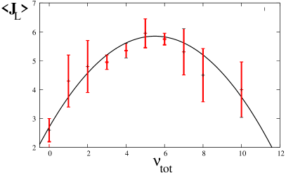
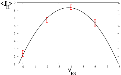
Figure 1: Average spins of FF for the Mo-Ba splitting up to $\nu=8$ as reported in [3].

In a joint effort with collaborators from Bucharest and Frankfurt, we addressed the special case of cold (neutronless) fission in view of its resemblance to cluster radioactivity [4]. In ref.[5] we assumed a scenario where the bending oscillations alone are responsible for angular momentum generation in fragments. Within the bending model the final angular momentum of each fragment is built up at scission and its generation is due solely to quantum fluctuations of the fragments orientation with respect to the strongly polarized fission axis. In this picture, angular momentum of FF carry unaltered fingerprints of the scission configurations (deformation of fragments and distribution of intrinsic excitatations among the fragments).

2 Spins of FF at scission

By scission point we understand in what follows a configuration where the fragments, while still in touch, have well-defined shapes, whether they are formed in their ground states like in cold fission or are elongated in the direction of the fission axis according to the way excitation energy is shared among fragments. In other words we adopt a cluster-like approach to fission as we did previously for cold fission [5]. In order to study the population of rotational states in the fission partners we have to take into account the deformation of nuclei and therefore establish the shape of the heavy-ion potential in the ”orientation landscape”, a task that we accomplish by appealing to the double-folding method. In this framework the separation of the radial from the angular coordinates in the potential is carried out by means of Fourier techniques as explained in detail in our earlier work [6] .

The calculation of the deformation energy at scission and the distribution of excitation energy among fragments is done by means of a general recipe which consists in determining first the ratio of prompt neutron numbers emitted by complementary fragments and then equate it to the ratio of fission fragment excitation energies. We employ a very recent analysis of the systematic behavior of experimental $\nu=\nu_{L}+\nu_{H}$ ($\nu_{H}/\nu$ as a function of $A_{H}$) [7]. Once $\nu_{L}$ and $\nu_{H}$ are determined the following relations between the excitation energy of complementary, fully accelerated fragments, and the total excitation energy $TXE$ are used

$$E_{H,L}^{*}=\frac{\nu_{H,L}}{\nu}TXE$$ (1)

We assume that at scission the excitation is accounted by the energy stored in the fragments deformation and a proportionally smaller contribution spent on the excitation of intrinsisc degrees of freedom

$$TXE=E_{\rm def}+E_{\rm sc}^{*}$$ (2)

The deformation energy is taken as the sum of liquid drop and shell model corrections energy

$$E_{\rm def}=\sum_{i=L,H}(E_{\rm LDM}^{i}+\delta W_{\rm shell}^{i})$$ (3)

The LDM part is taken as the sum of a surface and Coulomb contributions only (the volume energy is taken to be independent of deformations) for a sharp-edge distribution of nuclear matter relative to the value for a sphere. To estimate it we appeal to the embedded spheroid model [8] . As for the shell corrections we apply the expeditive procedure of Myers and Swiatecki [9] .

The content of $E_{\rm sc}^{*}$ is assumed to be accounted soleley by the excitation of collective rotational states of the FF. This quantity amounts to a few MeV regardless of the total number of emitted neutrons.

Following the spirit of the bending model [5], we assume that at scission the elongation (translational) degree of freedom $R=R_{\rm sc}$ is nailed down, and the FF can execute only angular vibrations around a direction perpendicular to the fission axis. Consequently the relevant degrees of freedom are the angular deviations $\theta_{1(2)}$ of the FF from the fission axis. The quantized bending Hamiltonian can be read off from eq.(18), ref.[5]

$$H_{\rm bend}=~{}-\frac{\hbar^{2}}{2{\cal B}_{1}}\frac{\partial^{2}}{\partial\theta_{1}^{2}}~{}-\frac{\hbar^{2}}{2{\cal B}_{2}}\frac{\partial^{2}}{\partial\theta_{2}^{2}}~{}-\frac{\hbar^{2}}{\mu R_{\rm sc}^{2}}\frac{\partial^{2}}{\partial\theta_{1}\partial\theta_{2}}~{}+~{}W_{\rm int}(\theta_{1},\theta_{2})$$ (4)

where ${\cal B}_{1(2)}$ are related to the inertia moments of the fragments, ${\cal J}_{1(2)}$

$${\cal B}_{1(2)}=\frac{{\cal J}_{1(2)}\mu R_{\rm sc}^{2}}{{\cal J}_{1(2)}+\mu R_{\rm sc}^{2}}.$$ (5)

In the Hamiltonian (4) we take into account only the deformed part of the potential, i.e. we discard the monopole term

$$W_{\rm int}(\theta_{1},\theta_{2})={1\over 2}C_{1}\theta_{1}^{2}+{1\over 2}C_{2}\theta_{2}^{2}+C_{12}\theta_{1}\theta_{2}$$ (6)

which is obtained by expanding (17) up to quadratic terms in powers of the polar angle $\theta.$ The explicit form of the stiffness parameters is [5].

$$C_{1,2} = -{1\over 2}\sum_{\lambda_{1}\lambda_{2}\lambda_{3}}~{}\lambda_{1,2}(\lambda_{1,2}~{}+1)V_{\lambda_{1}\lambda_{2}\lambda_{3}}^{0~{}0~{}0}(R_{\rm sc})$$ (7)

$$C_{12} = -{1\over 4}\sum_{\lambda_{1}\lambda_{2}\lambda_{3}}\left\{\lambda_{3}(\lambda_{3}~{}+1)-\lambda_{1}(\lambda_{1}~{}+1)-\lambda_{2}(\lambda_{2}~{}+1)\right\}V_{\lambda_{1}\lambda_{2}\lambda_{3}}^{0~{}0~{}0}(R_{\rm sc})$$ (8)

The bending Hamiltonian, consisting of two coupled Hamiltonians, can be reduced to the canonical form by means of a unitary transformation of exponent

$$S=\theta_{1}\frac{\partial}{\partial\theta_{2}}-\frac{K_{p}\omega_{2}^{2}+K_{q}}{K_{p}\omega_{1}^{2}+K_{q}}\theta_{2}\frac{\partial}{\partial\theta_{1}}$$ (9)

where

$$\omega_{1(2)}=\sqrt{C_{1(2)}\over{\cal B}_{1(2)}},~{}~{}~{}~{}~{}~{}K_{q}=\frac{C_{12}}{\sqrt{{\cal B}_{1}{\cal B}_{2}}},~{}~{}~{}~{}~{}~{}~{}K_{p}=\frac{\sqrt{{\cal B}_{1}{\cal B}_{2}}}{\mu R_{\rm sc}^{2}}.$$ (10)

The eigenvalues of the uncoupled Hamiltonian have the usual form

$$E_{n_{1}n_{2}}=\hbar\Omega_{1}\left(n_{1}+{1\over 2}\right)+\hbar\Omega_{2}\left(n_{2}+{1\over 2}\right)$$ (11)

where the relation between the new frequencies $\Omega_{i}$ and the old ones $\omega_{i}$, if we choose $\omega_{1}>\omega_{2}$, is given by

$$\Omega_{1(2)}^{2}=\frac{\left(K_{q}(\omega_{1}^{2}+\omega_{2}^{2}\pm\sqrt{\Delta})+2K_{p}\omega_{1}^{2}\omega_{2}^{2}\right)\left(K_{p}(\omega_{1}^{2}+\omega_{2}^{2}\pm\sqrt{\Delta})+2K_{q}\right)}{4(K_{p}\omega_{1}^{2}+K_{q})(K_{p}\omega_{2}^{2}+K_{q})}$$ (12)

with

$$\Delta=(\omega_{1}^{2}-\omega_{2}^{2})^{2}+4(K_{p}\omega_{1}^{2}+K_{q})(K_{p}\omega_{2}^{2}+K_{q})$$ (13)

In the bending picture the angular momentum of each fragment is calculated as square-roots of the ground state ($(n_{1},n_{2})=(0,0)$) expectation values of the operators $L_{k}^{2}=-\hbar^{2}\partial^{2}/\partial\theta_{k}^{2}(k=1,2)$ [5].

3 Evolution of FF spins during the post-scission stage

In the post-scission stage, the decay of ²⁵²Cf in two fragments is described by the the distance between the fragments centers $R$ which stands for the elongation of the system undergoing fission and by he orientation in space $\Omega_{i}$ of each rotator.

Fragment deformations ($\beta_{i}$) are considered as parameters of the dynamical problem and they preserve the value calculated at scission for a given excitation energy. In what follows we are going to specify the fragment-to-fragment distance $R$ as a variable depending parametrically on time, i.e. $R=R(t)$.

Accordingly, the dynamical problem is formulated in terms of a Hamiltonian where the translational and rotational motion are coupled only via the deformed part of the potential.

$$H_{\rm fiss}=\frac{1}{2}{\mu\dot{R}^{2}}+V_{0}(R)+H_{\rm rot}(\Omega_{1})+H_{\rm rot}(\Omega_{2})+W_{\rm int}(R,\Omega_{1},\Omega_{2})$$ (14)

In the above formula the first term represents the translational kinetic energy that asymptotically coincides with the observed kinetic energy $TKE(\infty)$, i.e.

$$TKE=Q-TXE$$ (15)

whereas

$$H_{\rm rot}(\Omega_{1,2})=\frac{\mbox{\boldmath$L$}_{1}^{2}}{2{\cal J}_{\rm 1,2}}$$ (16)

are the free rotational Hamiltonians of the fragments with angular momentum $\mbox{\boldmath$L$}_{i}$. The non-trivial part of our fission Hamiltonian is represented by the deformed part of the interaction from which we substracted the monopole-monopole interaction $V_{0}$ (see [6] for the derivation) :

$$W_{\rm int}(R(t),\Omega_{1},\Omega_{2})=\sum V_{\lambda_{1}\lambda_{2}\lambda_{3}}^{\mu-\mu 0}(R(t))D_{\lambda_{1}0}^{\mu}(\Omega_{1})D_{\lambda_{2}0}^{-\mu}(\Omega_{2})-V_{0}(R(t))$$ (17)

Whereas the standard approach [10] to Coulomb excitation (Coulex) assumes that the relative motion of the centers of mass of the two reacting nuclei can be described clasically, in the present approach we calculate the time-evolution of a quantum wave-packet across the Coulomb+nucler barrier. Note that in the case of Coulex the classical assumption for the trajectory $R(t)$ is justified by large impact parameters. This has the obvious consequence that the two nuclei do not get into the domain of nuclear interation and therefore the quantum tunneling across the reciprocal fusion barrier plays no role. For that reason we stick to the other approximation used in the Coulex case, namely that the energy transfer between the two nuclei is negligible. This assumption is likely to be valid in fission, since it seems to be not unreasonable that after scission the fragments are only weakly redistributing the excitation energy stored in intrinsic motion; excitation energy stored in deformation is shared between fragments at scisssion and do not get changed afterwards as we alredy remarked above. Since the translational energy exceeds by far the energy distributed on the excited rotational states (approximately a factor of 100), it is justified to assume that quantum tunneling is the dominant part of the Hamiltonian and its dynamics can be resolved separately from the one corresponding to the rotational degrees of freedom.

In support of the above assumption we should also mention that due to the barrier thickness, at least in the quantum tunneling regime, $R(t)$ represents the slow degree of freedom. The period of bending oscillations is much shorter than the time necessary for the wave packet average position to cover the distance between the first and the second turning point.

Under such circumstances the relative motion of the two flying apart fragments is not affected by the excitation of rotational levels in the two rotating fragments and therefore the total wave-function is given by the direct product of radial and rotational wave functions:

$$\Psi\sim\psi(R,t)\otimes\Phi(\Omega_{1},\Omega_{2};R(t))$$ (18)

Note that in the rotational wave-function, $R(t)$ appears as a parameter.

The relative motion is governed by the time-dependent Schrödinger equation in this degree of freedom

$$i\hbar\frac{\partial\psi(R,t)}{\partial t}=\left\{-\frac{\hbar^{2}}{2\mu}\nabla_{\mbox{\boldmath$R$}}+V_{0}(\mbox{\boldmath$R$})\right\}\psi(R,t)$$ (19)

The initial wave-packet is prepared as a bound state of energy $TKE$, in the spherical potential $V_{0}(R)$ for a two-body system of reduced mass $\mu$, i.e.

$$-\frac{\hbar^{2}}{2\mu}\Delta_{\mbox{\boldmath$R$}}\psi(R,0)+V_{0}(R)\psi(R,0)=TKE\psi(R,0)$$ (20)

and next it is propagated in time by applying the Crank-Nicolson scheme as we did in previous publications on $\alpha$-decay [11] and cold fission [12]. The quantum trajectory $R(t)$ can now be extracted from the knwoledge of the wave-packet $\psi(R,t)$ at any moment of time,

$$R(t)=\int_{0}^{\infty}d~{}R~{}R~{}|\psi(R,t)|^{2}$$ (21)

Note that the evolution of the wave-packet is determined for a time long enough to include not only the sub-barrier, but also the pure Coulomb part of the trajectory.

In view of the factorization (18) the time-dependent Schrödinger equation describing the coupled dynamics of the two rotators reads

$$i\hbar\frac{\partial\Phi(t)}{\partial t}=\left[H_{0}+W_{\rm int}(t)\right]\Phi(t)$$ (22)

where $H_{0}$ is the Hamiltonian of the free (uncoupled) rotators wich satisfying the eigenvalue problem

$$H_{0}\mid(I_{1}M_{1})(I_{2}M_{2})\rangle=E_{I_{1}I_{2}}\mid(I_{1}M_{1})(I_{2}M_{2})\rangle$$ (23)

$I$ and $M$ are the spin and the magnetic quantum number respectively. In what follows we resort to the approximation $M_{1}=M_{2}=0$, used also in the framework of the bending model, and justified by the strong polarization of fragments at the scission moment ($t=0$). In this configuration the spin of each fragment is oriented along an axis perpendicular to the fission axis [6] and its projection on the fragment $z$-axis is nil.

The matrix elements of the interaction in the basis $\mid I_{1}I_{2}\rangle$ are readily calculated using standard angular algebra techniques

$$\langle I_{1}I_{2}\mid W_{\rm int}\mid I^{\prime}_{1}I^{\prime}_{2}\rangle = \frac{1}{4\pi}\frac{{\hat{I}}_{1}{\hat{I}}_{2}}{{\hat{I}^{\prime}_{1}}{\hat{I}^{\prime}_{2}}}\times$$

$$\sum_{\lambda_{1}+\lambda_{2}+\lambda_{3}\geq 4}{\hat{\lambda}_{1}}{\hat{\lambda}_{2}}{V}_{~{}\lambda_{1}\lambda_{2}\lambda_{3}}^{~{}0~{}0~{}0}(R)\left(C^{I_{1}\lambda_{1}I^{\prime}_{1}}_{0~{}0~{}0}\right)^{2}\left(C^{I_{2}\lambda_{2}I^{\prime}_{2}}_{0~{}0~{}0}\right)^{2}$$

To solve eq.(22), $\Phi(t)$ is expanded in eigenstates of $H_{0}$, i.e.

$$\Phi(t)=\sum_{I_{1}I_{2}}{a}_{I_{1}I_{2}}(t)e^{-\frac{i}{\hbar}E_{I_{1}I_{2}}t}\mid I_{1}0\rangle\mid I_{2}0\rangle$$ (24)

and thus instead of solving a two-dimensional parabolic equation with a time-dependent potential, that provides a solution that has to be subsequently projected on each eigenstate $\mid I_{1}I_{2}\rangle$, we arrive at a coupled system of linear ordinary differential equations

$$i\hbar{\dot{a}}_{I_{1}I_{2}}(t)=\sum_{I^{\prime}_{1}I^{\prime}_{2}}\langle I_{1}I_{2}\mid W_{\rm int}\mid I^{\prime}_{1}I^{\prime}_{2}\rangle\exp{\left[i(E_{I_{1}I_{2}}-E_{I^{\prime}_{1}I^{\prime}_{2}})t/\hbar\right]}a_{I^{\prime}_{1}I^{\prime}_{2}}$$ (25)

The initial values $a_{I_{1}I_{2}}(0)$ are fixed by the spins evaluated at the scission point. In the basis we include up to 36 states, which means that in each fragment a state of maximum spin $I=14$ can be populated. Separating the real and imaginary components of the complex amplitude $a_{I^{\prime}_{1}I^{\prime}_{2}}$ we end-up with a system of 72 equations. Even in the case when we include multipoles up to $\lambda=6$ in the potential, a run on a standard computer takes less time than solving the partial differential equations (22). The amplitudes above depend on the quantum trajectory $R(t)$, which for thick barriers has a strongly oscillating behavior in the tunneling regime and then, outside the Coulomb barrier, tends asymptotically to the classical trajectory. In Fig.2 we plot the time evolution of the squared modulus amplitudes $\mid a_{I_{1}I_{2}}(t)\mid^{2}$. On the left panel we represented the neutronless ($\nu=0$) case. Since no energy is available for rotation at scission, the initial probability is concentrated in $a_{00}$ and therefore the rotational g.s. state $|00\rangle$ dominates mostly during the sub-barrier motion. When fragments are running in the pure Coulomb field, it will be overunned by higher spin states of the heavier fragment, e.g. $|04\rangle$ and $|02\rangle$. In the case with $\nu=2$ (right panel of Fig.2), the non-rotating state $|00\rangle$ decrease rapidly during the sub-barrier motion and displays some revivals (flashes) with smaller amplitude as time goes on. One should note that in the case of Coulomb excitation, when one deals with smooth non-oscillatory trajectories, there is a complete revival of the amplitudes [13] . In this case the population probability is higher in the light fragment, the states $|40\rangle$, $|20\rangle$ prevailing over $|04\rangle$ and $|02\rangle$

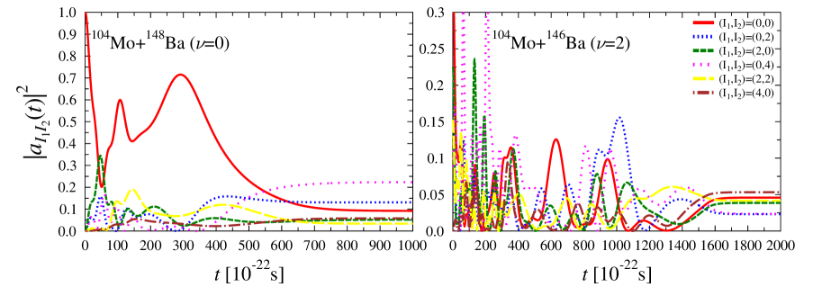
Figure 2: Evolution of the modules of the rotational states amplitudes.

The time-dependent average values of the spins are simply given in terms of the amplitudes

$$\langle J_{\rm L,H}^{2}\rangle=\sum_{I_{1}I_{2}}\mid a_{I_{1}I_{2}}(t)\mid^{2}I_{1,2}(I_{1,2}+1)$$ (26)

In Fig.3 the time evolution of the average momentum is displayed separately for the light fragment (left panel) and the heavy fragment (right panel) for 3 different excitation energies that correspond to $\nu=0,2,4$. We should note at this point that in our calculations we do not take into account any type of correction of the average momenta of the primary fragments for the loss from neutron evaporation. The data reported in [3] operates such a correction by using an evaporation calculation for the spin $j$ removed on average by one evaporated neutron. In that reference they reported calculated $j$ values for Ba and Mo varrying from $\sim 0.6\hbar$ to $\sim 0.3\hbar$ when $\nu_{L}$ changed from 1 to 6 and $\nu_{H}$ from 1 to 3. Even if we adopt the most simple assumption, i.e. each removed neutron carries away $j=1/2$, the fact that the average angular momentum increases for both fragments still hold according to Fig.3.

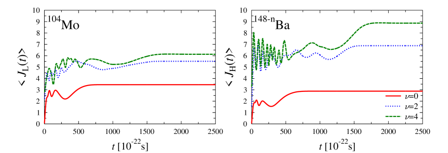
Figure 3: Evolution of average spins of the light (Mo) and heavy (Ba) fragments for total number of emitted neutrons $\nu=0,2,4$.

4 Conclusions

The fission dynamical model used in this study with the aim to estimate the average of spins of the emitted fragments consists of a traditional statical approach at scission, where the initial population of rotational is determined and subsequently is feeding a semiclasscial time-dependent coupled-system of equations for the occupation amplitudes of these states. The non-stationary quantum sub-barrier motion induces a strongly non-linear behavior of these amplitudes which eventually stabilizes to constant asymptotic values in the purely Coulomb field. Consequently the generation of angular momentum is the result of the complex dynamics after scission. Previous attempts, based exclusively on static models, that addressed the quest of how rotation is pumped into the intially ”frozen” fragments are in our opinion limited to a relatively early instance of the fission process and therefore cannot provide credible predictions for the final characteristics of the FF.

The model propsed in this work confirms the observed steady increase of the fragments rotation in spontaneous fission of ²⁵²Cf when going from 1 to 4 emitted neutrons. However, knowledge on the fragment configuration and energy content at scission can only indirectly be extracted from such an analysis.

The present approache is able to provide estimations also for other observables in binary fission such as the translational kinetic energy and can be extended to ternary fission.

References

- [1] A. A. Raduţa, Foundations of Nuclear Theory(in romanian), 2nd edn. (Univ.of Bucharest Publ.House, 2010).
- [2] J.H. Hamilton, A. V. Ramayya and H. K. Carter (eds.), Fission and Properties of Neutron-Rich Nuclei (World Scientific, Singapore, 2003).
- [3] G. S. Popeko et al., Rom.Jour.Phys. 47, 71 (2002)
- [4] A. Sandulescu, Ş. Mişicu, F. Carstoiu and W. Greiner, Phys.Part.Nucl, 30, 386 (1999).
- [5] Ş. Mişicu, A.Săndulescu, G.M. Ter-Akopian and W.Greiner, Phys.Rev C 60, no.3, 034613 (1999).
-
[6]
Ş. Mişicu and W. Greiner, J.Phys.G28, 2861 (2002).
Ş. Mişicu and W. Greiner, Phys.Rev.C66, 044606 (2002). - [7] C. Manailescu, A. Tudora, F. -J. Hambsch, C. Morariu and S. Oberstedt, Nucl.Phys.A867 12 (2011)
- [8] U. Brosa, S. Grossmann and A. Müller, Phys.Rep.197, 167 (1990).
- [9] W.D.Myers and W.J.Swiatec̆ki, Nucl.Phys.A81 (1966) 1
- [10] J. M. Eisenberg and W. Greiner, Nuclear Theory: Excitation Mechanisms of the Nucleus, vol. 2 (North-Holland, Amsterdam, 1970).
- [11] Ş. Mişicu, M. Rizea and W. Greiner, J.Phys.G:Part.&Nucl.27, 993 (2001).
- [12] Ş. Mişicu, A. Sandulescu and W. Greiner, Phys. Rev. C 64, 044610 (2001).
- [13] L. Fonda, N. Mankoc̆-Bors̆tnik and M. Rosina, Phys.Rep.158, 159 (1988)