Influence of asperities on fluid and thermal flow in a fracture: a coupled Lattice Boltzmann study

Abstract

The characteristics of the hydro-thermal flow which occurs when a cold fluid is injected into a hot fractured bedrock depend on the morphology of the fracture. We consider a sharp triangular asperity, invariant in one direction, perturbing an otherwise flat fracture. We investigate its influence on the macroscopic hydraulic transmissivity and heat transfer efficiency, at fixed low Reynolds number. In this study, numerical simulations are done with a coupled lattice Boltzmann method that solves both the complete Navier-Stokes and advection-diffusion equations in three dimensions. The results are compared with those obtained under lubrication approximations which rely on many hypotheses and neglect the three-dimensional (3D) effects. The lubrication results are obtained by analytically solving the Stokes equation and a two-dimensional (integrated over the thickness) advection-diffusion equation. We use a lattice Boltzmann method with a double distribution (for mass and energy transport) on hypercubic and cubic lattices. Beyond some critical slope for the boundaries, the velocity profile is observed to be far from a quadratic profile in the vicinity of the sharp asperity: the fluid within the triangular asperity is quasi-static. We find that taking account of both the 3D effects and the cooling of the rock, are important for the thermal exchange. Neglecting these effects with lubrication approximations results in overestimating the heat exchange efficiency. The evolution of the temperature over time, towards steady state, also shows complex behavior: some sites alternately reheat and cool down several times, making it difficult to forecast the extracted heat.

NEUVILLE ET AL. ASPERITIES INFLUENCE ON HYDROTHERMAL EXCHANGES E.G. Flekkøy, Advanced Material and Complex System group, Department of Physics, University of Oslo, PO BOx 1048, Blindern, Oslo 0316, Norway. (e.g.flekkoy@fys.uio.no) A. Neuville, Advanced Material and Complex System group, Department of Physics, University of Oslo, PO BOx 1048, Blindern, Oslo 0316, Norway. (amelie.neuville@fys.uio.no) R. Toussaint, Institut de Physique du Globe de Strasbourg, Université de Strasbourg/EOST, CNRS, 5 rue René Descartes, 67084, Strasbourg Cedex, France. (renaud.toussaint@unistra.fr)

1 Introduction

Conductive and convective transport of heat or chemical species, is omni-present in Earth sciences (Stephansson et al., 2004; Steefel et al., 2005), within porous or fractured media. Some technologies related to chemical transport, like radioactive storage (Cvetkovic et al., 2004; Amaziane et al., 2008; Halecky et al., 2011; Hoteit et al., 2004), or well acidizing, requires a good resolution of advection diffusion of chemical concentration (Szymczak and Ladd, 2009; Cardenas et al., 2007). The transport is influenced by the temperature which may play a role by modifying 1) the fluid transport – notably by natural convection, 2) the chemical constants of the reactions, or 3) the geometry of the porous medium. For instance some chemical reactions or rheological rock transformations only occur in given ranges of temperature (e.g. decarbonation, dehydration of sediments, decomposition of kerogen (e.g. Mollo et al., 2011; Petersen et al., 2010)). Thermal fracturing can result from chemical reactions generating gas (Kobchenko et al., 2011), or from thermal stress (Lan et al., 2012; Bergbauer et al., 1998), or from hydro-thermal stress, when injecting hot or cold fluid into a rock. Temperature monitoring is for example necessary to prevent potential damages of well installations. Apart from fracturing processes, other changes of geometry of the porous medium can also occur during injection of cold or warm fluid in Enhanced Geothermal Systems (EGS), because of poroelastic effects (Gelet et al., 2012), and also because of chemical reactions like acidizing. Exploitation of EGS requires also the heat exchange to be efficient and durable. An important step is, therefore, to understand the hydro-thermal coupling between fluid and rock; this is the aim of our present modeling.

Hydraulic transport mostly occurs in fractures. It was shown under lubrication approximations and steady state conditions, that the complexity of the fracture topography influences the hydro-thermal exchange when a cold fluid is injected into a hot fractured bedrock (Neuville et al., 2010). More specifically, the lubrication approximations state that the aperture and its wall topographies vary smoothly so that the velocity field is parallel to the main plane of the fracture (the component of the hydraulic flow perpendicular to the main fracture plane is neglected), and that the thermal diffusion only occurs in the directions perpendicular to the main plane of the fracture. For this modeling, the rock temperature was also supposed to be constant. In other models, as e.g. in the study of Natarajan and Kumar (2010), the heat diffusion in the rock is considered, but with a simplified fluid flow. Some features which are observed in nature, like fluid recirculation, and time-dependent temperature at the pumping well, can, however, not be explained with these model. We therefore wish to go beyond this lubrication assumption and be especially able to observe effects due to highly variable morphology of the fluid-rock interface. Indeed, even if many fluid rock interface topographies or fracture apertures are statistically self-affine (multi-scale property) (Brown and Scholz, 1985; Bouchaud, 1997; Neuville et al., 2012; Candela et al., 2009), it is very often possible to observe some isolated asperities with sharp variations of the topography, for instance along cleavage planes (Neuville et al., 2012), or due to particle detachment, or along stylolite teeth (Renard et al., 2004; Ebner et al., 2010; Koehn et al., 2012; Laronne Ben-Itzhak et al., 2012; Rolland et al., 2012). The roughness of the fracture can also be perturbed by intersection with other fractures (Nenna and Aydin, 2011), or, for microfractures, by the matrix porosity (Renard et al., 2009).

Investigations on the validity of the lubrication approximation, based on the study of some geometrical parameters have been performed e.g. by Zimmerman and Bodvarsson (1996); Oron and Berkowitz (1998); Nicholl et al. (1999). Without the lubrication approximation, i.e. with full solving of the Navier-Stokes equation, the hydraulic behavior in channels or fracture with sinusoidal walls were studied e.g. by Brown et al. (1995); Waite et al. (1998); Bernabé and Olson (2000) with lattice gas methods. It was shown that for a sinusoid with a short wavelength and large amplitude compared to the mean aperture, the hydraulic aperture is smaller than that expected with the lubrication approximation. Error on the hydraulic aperture computed with a lubrication approximation have been analytically obtained by Zimmerman and Bodvarsson (1996), and experimentally by Oron and Berkowitz (1998); Nicholl et al. (1999). In these studies, the fluid flow was reported to be important in the middle of the channel, while it is quasi-stagnant in the sharp hollows of the walls. Eddies were numerically observed in this quasi-stagnant zones (Brown et al., 1995; Brush and Thomson, 2003; Boutt et al., 2006; Cardenas et al., 2007; Andrade Jr. et al., 2004) in various fracture geometries, including realistic fracture geometries. These eddies are similar to those analytically predicted by Moffatt (1964), who studied eddies formation in a corner between two intersecting planes, when the flow is imposed to be tangential to the planes at an infinite distance from the corner. Microfluidics has also been investigated using LBM (e.g. Harting et al., 2010).

On the one hand, many studies exist about the coupling between the fully solved hydraulic behavior – solving of the Navier Stokes equation – and solute or particle transport, or dispersion in general (Boutt et al., 2006; Cardenas et al., 2007; Drazer and Koplik, 2001, 2002; Flekkøy, 1993; Yeo, 2001; Johnsen et al., 2006; Niebling et al., 2010; Vinningland et al., 2012).

On the other hand, few studies take into account the fully solved hydraulic flow with the heat transfer, when a cold fluid is injected into a fracture embedded in a hot solid. In the absence of flow, the stationary problem of heat transport accross a fractal interface was studied, e.g. by Grebenkov et al. (2007). Even if both, heat and solute transport, are described with advection-diffusion equation, many differences exist due to different boundary conditions and different range of parameters. Andrade Jr. et al. (2004) solved the temperature field when a warm fluid is injected within a two-dimensional (2D) channel delimited by walls whose topographies follow Koch fractals, using the “Semi-Implicit Method for Pressure Linked Equations” algorithm developed by Patankar (1980). In his study, the walls of the channel were however set at a constant temperature. Other studies regarding cooling issues of electrical devices have also been done (e.g. Young, 1998, and references therein), but in contrast to the current study, the thermal boundary conditions used in these works are less relevant for natural problems (for instance, insulated walls are used). Another branch of algorithms for heat solving are done with lattice Boltzmann methods (LBM). The LBM (e.g. Wolf-Gladrow, 2005) are very suitable to model the complexity of hydrothermal transport in a rough fracture morphology, whatever the slopes of the morphology (i.e., without any conditions on the smoothness of the morphology). As the algorithms require only local operations (while other numerical methods requires e.g. inversion of matrices depending on the geometry of the entire porous medium), they handle complex boundaries very well. Several methods have been proposed: multispeed scheme (a density distribution is used, with additional speeds and high order velocity terms in the equilibrium distribution), hybrid method (hydraulic flow is solved with LBM, and heat transport is solved with another method), and double distribution. A review of these methods can be found in Lallemand and Luo (2003); Luan et al. (2012). Most of the problems solved so far with LBM deal with benchmarks that consist in close systems (square cavity with impermeable walls). In this paper we will examine the limits of the lubrication approximation, and the model developed in Neuville et al. (2010). After briefly recalling the fundamentals of this model, we describe the numerical methods used for our modeling outside the lubrication approximations. We chose a LBM with a double distribution method, where the hydraulic flow is independent of the temperature. The chosen lattices for the flow and temperature variables are respectively hypercubic and cubic, with a single lattice speed for each lattice. This choice is seldom used in literature, but it is suitable for three-dimensional (3D) mass and heat transport modeling (d’Humières et al., 1986; Wolf-Gladrow, 2005; Hiorth et al., 2008). Despite the methods being implemented in 3D, for simplicity reasons, the parameter exploration is done in two dimensions, translational invariance being assumed along the third dimension. For a self-affine aperture, the contribution of each asperity on the total hydraulic and thermal exchanges is difficult to single out. For this reason, here, we chose as a simpler situation to focus on one single asperity where we can lead a precise quantitative study of the flow organization and properties in space and time as function of flow speed, asperity size and shape, and heat transport properties.

We will thus explore the behavior of the flow in a fracture with a triangular asperity, as function of the asperity size. We will compare the results directly to the lubrication approximation results, and establish when this one fails to model correctly the mass and heat transport.

2 Methods for hydro-thermal modeling

2.1 Solving under lubrication approximations

The lubrication approximation holds in the laminar regime, at small Reynolds number, for fluids flowing into a fracture whose aperture and both wall-topographies, show smooth variations. Under these assumption, the Navier-Stokes equation reduces to the Reynolds equation (Pinkus and Sternlicht, 1961; Brown, 1987):

$$\boldsymbol{\nabla}\cdot\left(a^{3}(x,y)\boldsymbol{\nabla}p\right)=0,$$ (1)

where $\boldsymbol{\nabla}p$ is the local 2D pressure gradient, and $a(x,y)$ is the fracture aperture. With $\hat{\boldsymbol{x}}$ (unitary vector) as the direction of the macroscopic pressure gradient, the velocity expresses as

$$\mathbf{u}(x,y,z)=\frac{\nabla p(x,y)}{2\eta}[z_{1}(x,y)-z][z-z_{2}(x,y)]\hat{\boldsymbol{x}},$$ (2)

where $z_{1}$ and $z_{2}$ are the out of plane coordinates of the fracture walls related to the aperture by $z_{2}-z_{1}=a$, and $\eta$ the dynamic viscosity of the fluid. The aperture of a fracture $a$ is partially characterized by its mean geometrical aperture, $A$, and by the standard deviation of the aperture. The hydraulic behavior can be partially characterized by the flow across the aperture, $\mathbf{q}$, defined as

$$\mathbf{q}=\int_{a(x,y)}\mathbf{u}(x,y,z)dz.$$ (3)

The hydraulic aperture $H$ is classically defined (Guyon et al., 2001) from the component of $\mathbf{q}$ along the macroscopic gradient direction, $q_{x}$:

$$H=\left(\langle q_{x}\rangle\frac{12\eta}{F}\right)^{\nicefrac{{1}}{{3}}},$$ (4)

where $F$ is the norm macroscopic pressure gradient, and $\langle.\rangle$ refers to the $x-y$ space averaging. For parallel plates geometry, $\mathbf{q}$ is a constant vector and $H=A$. The thermal behavior of a fluid injected in a fracture (with a self-affine aperture) embedded in a constantly warm rock was modeled in Neuville et al. (2010, 2011) under the so-called thermal lubrication approximation. In their solving, several terms are discarded in the heat equation: for instance the conduction occurs only perpendicularly to the fracture mean plane ($z$), and the convection is neglected along $z$. The thermal exchange balance in a stationary regime resumes in

$$\mathbf{q}\cdot\boldsymbol{\nabla}\overline{T}+2\frac{\chi_{f}}{a}\text{N\!u}\cdot\left(\overline{T}-T_{r}\right)=0,$$ (5)

where $\chi_{f}$ is the thermal diffusivity of the fluid, $\text{N\!u}={\pm\left.\frac{\partial T}{\partial z}\right|_{z=z_{1,2}}a}/({T_{r}-\overline{T}})$ is the Nusselt number, classically used to evaluate the thermal efficiency in reference with the conductive heat flow, and

$$\overline{T}\left(x,y\right)=\frac{\int_{a}u_{x}\left(x,y,z\right)T\left(x,y,z\right)dz}{q_{x}}$$ (6)

is a temperature averaged across the aperture, weighted by the velocity. For a parallel plates geometry, it can be shown, under assumptions over the temperature gradient, that $\text{N\!u}={70}/{17}$ (Turcotte and Schubert, 2002; Neuville et al., 2010). In this method, the temperature profile across the aperture follows a quartic law. It was shown (Neuville et al., 2010) that for a self-affine aperture, the averaged temperature law over the $y$ direction, $\overline{\overline{T}}$, defined as

$$\overline{\overline{T}}(x)=\frac{\int q_{x}\left(x,y\right)\overline{T}\left(x,y\right)/a(x,y)dy}{\int q_{x}\left(x,y\right)/a(x,y)dy},$$ (7)

can be approximated by

$$\overline{\overline{T}}-T_{r}=\left({T}_{f}^{0}-T_{r}\right)\exp\left(-\frac{x}{R}\right),$$ (8)

where ${T}_{f}^{0}=\overline{T}(x=0)$ is imposed at the inlet of the fracture, $T_{r}$ is the temperature of the wall (interface fluid-solid), and $R$ is a thermal length, obtained from a linear regression. For parallel plates separated by $A_{0}$, $R$ is equal to

$$R=\frac{A_{0}q}{2\text{N\!u}\chi_{f}}.$$ (9)

Note that any change of the thermal length can also be interpreted in term of Nusselt number variation.

2.2 Full solving, using coupled Lattice Boltzmann Methods (LBM)

2.2.1 Solving the mass transport with FCHC LBM

In LBM, fictitious particles move and collide on a lattice. Operations conserves mass and momentum at mesoscopic scale. Using appropriate rules and lattice topology, it can be shown that the Navier-Stokes equation can be recovered at macroscopic scale (e.g. Rothman and Zaleski, 1997; Chopard and Droz, 1998; Wolf-Gladrow, 2005). The distribution of mass density is denoted as $f_{i}$, where the index $i$ refers to the direction of propagation of the particles moving with a velocity $\boldsymbol{c_{i}}$ on the lattice. We choose a “Face-Centered-Hyper-Cubic” (FCHC) lattice. This is a four-dimensional lattice with suitable topological properties to solve the Navier-Stokes equation (d’Humières et al., 1986) in three dimensions. The $N=24$ vectors defining the lattice directions are $\boldsymbol{c_{i}}\frac{\delta t}{\delta x}$ $(\pm 1,\pm 1,0,0)$, $(0,\pm 1,\pm 1,0)$, $(0,0,\pm 1,\pm 1)$, $(0,\pm 1,0,\pm 1)$, $(\pm 1,0,\pm 1,0)$, $(\pm 1,0,0,\pm 1)$, with $c=\sqrt{2}\delta x/\delta t$, where $\delta t$ and $\delta x$ are the time and space steps. The total density and the macroscopic velocity $\mathbf{u}$ at each node $M$ are computed with ($\mathbf{O\!M}$ being the position vector):

$$\begin{split}\rho(t,\mathbf{O\!M})&=\sum_{i=1}^{24}{f_{i}}(t,\mathbf{O\!M})\\ \rho\mathbf{u}(t,\mathbf{O\!M})&=\sum_{i=1}^{24}{\boldsymbol{c_{i}}f_{i}}(t,\mathbf{O\!M}).\end{split}$$ (10)

For the collision phase, a standard BGK scheme (Bhatnagar, Gross, and Krook – Bhatnagar et al., 1954; Qian et al., 1992) is used. The linearized collision term depends on a constant of relaxation $\lambda$, which is linked to $\nu=\eta/\rho$ the kinematic viscosity of the fluid (Rothman and Zaleski, 1997) by:

$$\nu=-\frac{c^{2}\delta t}{6}\left(-\frac{1}{2}+{\lambda}\right).$$ (11)

The macroscopic pressure gradient between the inlet and outlet of the fracture is implemented through a volumetric force that intervenes during the collision phase at each lattice node.

It can be shown that the density of the fluid is linked to the velocity by $p=\rho(\delta x^{2}/(2\delta t)^{2}-u^{2}/4)$ (Rothman and Zaleski, 1997). This modeling of Navier-Stokes equation holds for compressible flows in the incompressibility limit, at small Mach number (ratio between the velocity and the sound speed on the lattice – here, equal to $u\delta t/(\sqrt{2}\delta x)$). The Knudsen number (ratio between the average distance between two collision, and the macroscopic scale of the system) should also be small.

2.2.2 Solving the heat transport with 3D cubic LBM

The transport of the heat is solved using a coupled lattice Boltzmann method, using a second particle distribution, $g_{i}$, which represents the internal energy distribution of the particles moving with the velocity $\mathbf{b}_{i}$. It is assumed that the heat is passively transported by the fluid: viscous heat dissipation is neglected, as well as the viscosity dependence with the temperature. Using square lattices and appropriate collision rules, it has been shown (Wolf-Gladrow, 2005; Hiorth et al., 2008) that the LBM solves advection-diffusion equation. The internal energy and its flux are conserved during the collision phase, which is done with a BGK scheme as in e.g. Hiorth et al. (2008) is used. We choose a 3D cubic lattice. Its $N_{T}=6$ base vectors, $\boldsymbol{b_{i}}\frac{\delta t}{\delta x}$, are defined by $(\pm 1,0,0)$, $(0,\pm 1,0)$, $(0,0,\pm 1)$ and $b=\delta x/\delta t$. This network is a sublattice of the 3D projection – perpendicularly to fourth direction – of the FCHC lattice. The temperature at each node $M$, and the internal energy flux are given by:

$$\begin{split}\sum_{i}^{N_{T}}g_{i}(\mathbf{O\!M},t)&=T(\mathbf{O\!M},t)\\ \sum_{i}^{N_{T}}\mathbf{b}_{i}g_{i}(\mathbf{O\!M},t)&=T(\mathbf{O\!M},t)\mathbf{u}\end{split}$$ (12)

2.2.3 LBM boundary conditions

Let consider a fractured medium, where the macroscopic pressure gradient in the fluid is aligned with the $\hat{\boldsymbol{x}}$ direction: the fluid injected at the inlet ($x=0$), and pumped out at the outlet of the system ($x=L_{x}$). The unitary vectors $\hat{\boldsymbol{x}}$, $\hat{\boldsymbol{y}}$ and $\hat{\boldsymbol{z}}$ define an orthonormal frame, and this porous medium is discretized with a cubic mesh. The center of each mesh is a fluid or a solid node.

The porous medium geometry and the flow are supposed to be periodic in $x$ and $y$. At the interface between the fluid and the solid, non slip boundary condition are chosen. This is implemented using the full-way bounce back boundary condition (Rothman and Zaleski, 1997) for the mass particle distributions. This bounce back operation is done for particle distributions $f_{i}(\mathbf{O\!M})$ where $M$ is a solid node, and $\mathbf{O\!M}+\boldsymbol{c_{i}}\delta t$ is in the fluid. For these nodes, the mass distributions $f_{i}$ of the bounce-backed nodes are exchanged with $f_{i+12}$, where the direction $i+12$ is opposite to the direction $i$. This is done instead of a collision operation. The propagation phase is then done normally on these nodes. For this bounce-back boundary condition, the interface fluid solid is supposed to be located half-way between the bounce-backed node and the fluid nodes (Fig. 1).

Figure 1: Discretization of the interface between the solid and fluid. The dots indicate the nodes of the lattice. BB stands for nodes in light gray where some particle distributions are bounce backed.

The temperature field is supposed to be periodic along $y$ direction. The temperature is imposed in $x=0$, $z=0$, $z=L_{z}$, where $L_{z}$ is the height of our system in the $z$ direction. In this study, the rock is maintained at temperature $T_{r}^{0}=150\text{\textdegree{}C}$ at the borders in $z=L_{z}$ and $z=0$. At the inlet of the system, in $x=0$, the rock and fluid are maintained respectively at $T=T_{r}^{0}$, and $T=T_{f}^{0}=30\text{\textdegree{}C}$. At the outlet of the system, the temperature is forced to $T=T_{r}^{0}$ at solid nodes (Dirichlet condition), and $T(x=L_{x})=T(x=L_{x}-\delta x)$ in liquid (von Neumann condition). In our program, the temperature at these nodes is imposed through an “equilibrium scheme” (Huang et al., 2011): at the end of each time step, and at the next collision step, the equilibrium distributions $g_{i}$ of these boundary nodes is set at the next collision step to the equilibrium distribution $g_{i}^{\text{eq}}$, with the desired temperature. For the nodes located at the outlet in the fluid, our boundary condition is equivalent, at first order, to zero temperature gradient along the $x$ direction. The systems considered are long enough so that the beginning of the systems is almost not influenced by outlet conditions (this boundary condition only creates a local artifact at the outlet). At the initial time, the rock and fluid have a temperature of respectively $T_{r}^{0}$ and $T_{f}^{0}$.

3 Geometry and hydro-thermal regime studied

We focus on the hydrothermal behavior within a fracture with a very simple geometry: it is a fracture with flat walls parallel to the $x-y$ plane, perturbed by a single asperity with sharp edges (Fig. 2). The fracture aperture $a(x)$ is invariable along the $y$ direction. In cross-view ($x-z$ plane), the asperity has a triangle shape characterized by its width $L$, depth $d$, and abscissa position $x_{0}$:

$$a(x)=A_{0}+d\>\Lambda\left[\!\!\;\!\frac{2}{L}\left(x-x_{0}-L/2\right)\right],$$ (13)

where $\Lambda$ is the unitary triangle function:

$$\Lambda(x)=\begin{cases}0,&\left|x\right|\geq 1\\ 1-\left|x\right|,&\left|x\right|<1.\end{cases}$$ (14)

For all the computations done with LBM in this study, the fracture is embedded in a solid whose dimension are $(L_{x},L_{z})=(200\text{~{}mm},89.5\text{~{}mm})$. This medium can be completely seen in Fig. 4a. The bottom wall of the fracture intersects the $x-z$ plane in $z=39.75\text{~{}mm}$, and the asperity is characterized by $(A_{0},x_{0})=(10\text{~{}mm},5\text{~{}mm})$, while $d$ and $L$ vary. The lattice discretization is $\delta x=0.5\text{~{}mm}$ and $\delta t=0.1250\text{~{}s}$.

The LBM simulations are done at low Reynolds number: $\text{R\!e}=0.17$, where it is computed as $\text{R\!e}={2Au_{M}}/({3\nu})$ with $u_{M}$ being the maximum velocity within a flat fracture separated by two parallel plates, of aperture $A_{0}$, estimated from the classical cubic law $u_{M}=FA_{0}^{2}/(8\eta)$ (Guyon et al., 2001).

For the thermal parameters, two different thermal diffusivity values are used in LBM for the fluid and the solid. The ratio of both, $\chi_{r}/\chi_{f}=0.17$, corresponds to the typical ratio of diffusivity values for crystalline rocks (of order of $1\text{~{}mm}^{2}$/s (Drury, 1987)) and water (at $100\text{\textdegree{}C}$, $0.17\text{~{}mm}^{2}$/s – (Taine and Petit, 2003)). The Péclet number, defined as $\text{P\!e}=u_{M}A/\chi_{f}$ is set to 45.96. The orders of magnitude of Reynolds and Péclet numbers that we use are compatible with the lubrication approximations.

4 Results: example of application

4.1 Illustration of the hydraulic behavior

4.1.1 Hydraulic lubrication approximation for a triangular asperity

The lubrication velocity is computed using Eq. (2). For an aperture which is invariant along $y$, the Reynolds equation Eq. (1) simplifies to

$$\partial_{x}p=K/a(x)^{3},$$ (15)

and the hydraulic flow is constant:

$$\mathbf{q}=-K/(12\eta)\hat{\boldsymbol{x}},$$ (16)

where $K$ is a constant. By integrating the pressure gradient between the inlet and outlet of the fracture, one gets

$$K=-{FL_{x}}\left({\int_{0}^{L_{x}}a^{-3}(x)dx}\right)^{-1},$$ (17)

where $\boldsymbol{F}$ is the pressure gradient imposed between the inlet and outlet of the fracture. $K$ is calculated analytically for the considered geometry (Eq. (13)), by noticing that:

$$\int_{0}^{L_{x}}\frac{dx}{a^{3}(x)}=\frac{-3A_{0}dL-2d^{2}L+2A_{0}^{2}L_{x}+4A_{0}dL_{x}+2d^{2}L_{x}}{2A_{0}^{3}(A_{0}+d)^{2}}.$$ (18)

4.1.2 Fully resolved hydraulic behavior compared to the lubrication approximation

Let’s first comment on the precision of the lattice Boltzmann (LB) results. We have some errors that come from the chosen implementation of the boundary conditions combined to the type of LBM. Because the fluid is slightly compressible with LBM, the averaged flow $q_{x}$ is not constant (the relative standard deviation of $q_{x}$ is around 0.39% for this example), and therefore the hydraulic aperture slightly varies according to the $x-$domain where it is computed. We chose to compute $H$ at the asperity scale, i.e. for $x_{0}\leq x\leq x_{0}+L$. For the case of a parallel flat wall fracture separated by $A_{0}=10\text{~{}mm}$, with a flow characterized by $\text{R\!e}=0.17$, solved with steps $\delta x=0.5\text{~{}mm}$, and $\delta t=0.125\text{~{}s}$, the absolute error on the computed velocity, defined as $E_{a}=\langle\left(u_{x}^{\text{L\!B}}-u_{x}^{l})\right)^{2}\rangle^{1/2}$ is $5.36\,10^{-4}\text{~{}mm/s}$. The relative error, defined as $E_{r}=E_{a}/\langle u_{x}^{l}\rangle$ is 3.22%. The relative error on the hydraulic aperture computed in this case is 1.11%. In order to take into account this numerical error, the comparison between LB and lubrication results is done using normalized hydraulic apertures. The hydraulic aperture obtained from the LBM calculation, and the one obtained from the lubrication approximation are respectively normalized in this way $H_{\text{L\!B}}^{*}=H_{\text{L\!B}}/H^{/\!/}_{\text{L\!B}}$ and $H_{\text{l\!u\!b}}^{*}=H_{\text{l\!u\!b}}/H^{/\!/}_{\text{l\!u\!b}}$. $H^{/\!/}_{\text{L\!B}}$ and $H^{/\!/}_{\text{l\!u\!b}}$ are the hydraulic apertures in parallel plate geometry, computed respectively with the LBM (discretized aperture), and with the lubrication approximation. We note also an error on the direction of the velocity vectors in the deepest part of the corner, for velocity vectors whose norm are of order $10^{-5}$ mm/s, i.e. very low velocity compared to the average velocity (see Fig. 2). In the zones where artefacts at very low velocities were observed, the thermal exchange is mainly led by diffusive exchanges. Therefore, we estimate that the error in the direction does not influence much the thermal exchange. Note that lattice Boltzmann methods with better precision are also available, like those with a modified equilibrium distribution (He and Luo, 1997), or those with two relaxation times (e.g. Talon et al., 2012).

Figure 2a shows the velocity norm under lubrication approximation (cross-section view), for a fracture with an asperity characterized by $(d,L)=(20\text{~{}mm},50\text{~{}mm})$. This has to be compared with Fig. 2b which shows the velocity norm and vectors at steady state across the fracture aperture, computed with the LBM. The difference of the velocity norms is in addition shown in Fig. 3a. In this configuration, the fluid flows within the asperity, and the main flow direction changes gently in accordance with the topography of the walls. The velocity field fully resolved and the one solved with the lubrication approximation show some similarities. However, some details are not captured with the lubrication approximation, notably in the deepest part of the corner where the full computation locally shows fluid at rest. It is computed that $H_{\text{L\!B}}^{*}=1.06$ and $H_{\text{l\!u\!b}}^{*}=1.07$ for the geometry shown in Fig. 2a, with $(d,L)=(20\text{~{}mm},50\text{~{}mm})$. Those values only differs by 1.15% i.e. the lubrication approximation still holds on average.

Let depart further from the smooth geometry where the lubrication assumptions apply. The same geometry as previously is used, but $L$ is set to $L=10\text{~{}mm}$, so that the geometry has a steeper topography. Similarly to Figs. 2a-b, Figs. 2c-d respectively show the lubrication and fully resolved velocity fields. Here, it is very clear that both are very different (see also Fig. 3b). In the asperity, a separation zone is observed: the fluid velocity is very small, and Fig. 2e shows that the fluid recirculates as if being trapped. The velocity profile is consequently very different from a quadratic profile as in Eq. (2). For the geometry shown in Figs. 2c-d $(d,L)=(20\text{~{}mm},10\text{~{}mm})$, it is computed that $H_{\text{l\!u\!b}}^{*}=1.01$ and $H_{\text{L\!B}}^{*}=1.00$. Therefore, it means that macroscopically the lubrication approximation is still a good estimation is this case. It is however clear that locally, within the asperity, the lubrication approximation is not valid.

Fractures with a bump (asperity with $d<0$) that reduces the aperture, are also investigated. Figs. 2f-g show the lubrication, and fully resolved velocity fields. The main differences are the two small separation zones with low velocities that appear just before and after the bump (Fig. 3c), in the corners with obtuse angles. This tiny asperity reduces the hydraulic aperture of 3.0%, with $H_{\text{L\!B}}^{*}=0.96$ and $H_{\text{l\!u\!b}}^{*}=0.98$.

Figure 2: (Color online) (a) Cross section view of the velocity norm (unit of the color scale: mm/s) under lubrification approximation ($u=u_{x}$). The shape of the asperity is defined by $(d,L)=(20\text{~{}mm},50\text{~{}mm})$. (b) Velocity vectors and their norm in color, with LBM. Same color scale as Fig. 2a. (c, d) Same as (a, b) for $(d,L)=(20\text{~{}mm},10\text{~{}mm})$. (e) Zoom of (d) with a different color scale, and the normalized velocity vectors $\mathbf{u}(x,z)/\left\|u\right\|$ superimposed. (f, g) Same as (c, d, e) for a bump asperity: $(d,L)=(-5\text{~{}mm},5\text{~{}mm})$. The scaling used to represent the vectors is six times smaller for (f, g) than for (c, d) and (a, b).

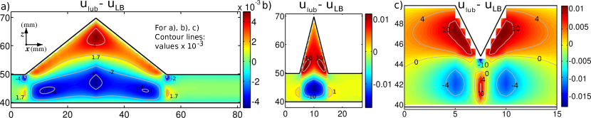
Figure 3: (Color online) Cross section view of the difference of the velocity norms obtained with lubrication and with LBM, for the geometries shown in Fig. 2

4.2 Illustration of the thermal behavior

4.2.1 Thermal lubrication approximation for a triangular asperity

For an aperture which is invariant along $y$, the hydraulic flow $\mathbf{q}$ is constant (Eq. (16)), and $\overline{\overline{T}}=\overline{T}$. By assuming that the rock temperature $T_{r}$ is constant, Eq. (5) simplifies into a first order linear ordinary differential equations with constant coefficients which has for solution (in a stationary regime):

$${\overline{T}}-T_{r}=\left({T}_{f}^{0}-T_{r}\right)\exp\left(-\int^{x}_{0}\frac{A_{0}}{a(\xi)R}d\xi\right).$$ (19)

For the considered geometry (Eq. (13)), $\int^{x}_{0}({a(\xi)})^{-1}d\xi$ can be computed analytically and expressed as a function of $R$ (Eq. (9)). The solution $\overline{T}^{*}=(\overline{T}-T_{r})/({T}_{f}^{0}-T_{r})$, is:

$$\begin{cases}e^{-\frac{x}{R}},&0\leq x\leq x_{0}\\ e^{-\frac{x_{0}}{R}}\left[1+\frac{2d(x-x_{0})}{A_{0}L}\right]^{-\frac{LA_{0}}{2dR}},&x_{0}\leq x\leq x_{0}+\frac{L}{2}\\ e^{-\frac{x_{0}}{R}}\left[\frac{A_{0}(A_{0}L+2d(L-x+x_{0}))}{L(A_{0}+d)^{2}}\right]^{\frac{LA_{0}}{2dR}},&x_{0}+\frac{L}{2}\leq x\leq x_{0}+L\\ e^{\frac{L-x}{R}}\left(\frac{A_{0}}{A_{0}+d}\right)^{\frac{LA_{0}}{dR}},&x_{0}+L\leq x\leq L_{x}.\end{cases}$$ (20)

This solution is shown in plot (a) of Fig. 5 and (a’, b’, c’) of Fig. 6, where $\ln\overline{T}^{*}$ as a function of $x$ is plotted for several geometries. Within the lubrication approximation, the slope of $\ln\overline{T}^{*}$ as a function of $x$ (Eq. (20)) is the same before and after the asperity, (i.e. for $x\leq x_{0}$ and for $x\geq x_{0}+L$) and it is given by $1/R$, where $R$ is defined in the lubrication regime with Eq. (9), $q$ being computed from Eqs. (16) to (18). Both straight lines have however different ordinates at the origin. This comes from the complicated behavior within the asperity zone. As a consequence the fit of $\ln\overline{T}^{*}(x)$ with a single straight line, following Eq. (8), clearly does not capture the details of the thermal exchange. In Fig. 6e, the linear fits done for the restricted range $0\leq x\leq 55$ mm (in the vicinity of the inlet) are shown. The negative inverse of the slope of these fits is named $R_{1\,\text{l\!u\!b}}$ (reported values in Tab. 1), and it can be compared to the $R$ values. For hollow asperities ($d>0$), $R_{1\,\text{l\!u\!b}}>R$. It means that, according to this solution, the heat exchange efficiency is reduced around the corner, compared to the heat exchange efficiency far from the corner. On the contrary, for bumps $d<0$, $R_{1\,\text{l\!u\!b}}<R$. The linear fit of the second part (far from the inlet), for $55\leq x\leq 150$ mm, results in a thermal length $R_{2\,\text{l\!u\!b}}$ analytically always equal to $R$. Indeed, since $x_{0}$ and $L$ values fulfill, by choice, $x_{0}+L\leq 55$ mm, this second fit is systematically done after the asperity.

4.2.2 Fully resolved thermal behavior compared to the lubrication approximation

In this subsection, we first comment qualitatively on the maps of the temperature obtained with LBM for few different asperities, in a stationary regime. The comparison to the lubrication approximation is then done quantitatively using average temperatures curves, from which thermal lengths are computed. The transient regime is also discussed at the end of this subsection.

Figure 4 shows the temperature map at steady state corresponding to the hydraulic behavior illustrated in Fig. 2. The shape of the isotherm lines within the fluid are strongly correlated with the hydraulic flow. For $(d,L)=(20\text{~{}mm},50\text{~{}mm})$, the cold fluid is clearly advected into the asperity. On the contrary, for $(d,L)=(20\text{~{}mm},10\text{~{}mm})$, the deepest part of the asperity is not affected by the injection of the cold fluid (very low velocities in this separated flow zone), and it heats up fast by conduction. As a consequence, the fluid within this second channel is warmer (ex. compare isolines $T=80\text{\textdegree{}C}$ on Figs 4a-b. For the narrower fracture, Fig. 4c, with $(d,L)=(-5\text{~{}mm},5\text{~{}mm})$, the reduction of the hydraulic flow ($H_{\text{L\!B}}^{*}=0.96$ and $H_{\text{L\!B}}^{*}=1.06$ respectively for $(d,L)=(-5\text{~{}mm},5\text{~{}mm})$ and $(d,L)=(20\text{~{}mm},50\text{~{}mm})$) inhibits the propagation of the cold fluid. This fluid consequently heats up in a shorter distance (better conductive transport) than for the two other cases. The rock cools down by conduction: the wall temperature is inferior to the rock temperature at the border of the system (150°C), especially where the rock is surrounded by cold fluid, for instance in Fig. 4c, at $(x,z)=(10\text{~{}mm},45\text{~{}mm})$.

Figure 4: Temperature maps at steady state for various asperity shapes: (a) $(d,L)=(20\text{~{}mm},50\text{~{}mm})$, (b) $(d,L)=(20\text{~{}mm},10\text{~{}mm})$, (c) $(d,L)=(-5\text{~{}mm},5\text{~{}mm})$. The black lines delimits the fracture embedded in the rock. The gray lines are isotherm lines (80, 100, 120 and 140°C).

The thermal behavior is now quantified in the same way as done in Neuville et al. (2010, 2011), i.e. by computing $\overline{T}^{*}$ (Fig. 5) as in Eq. (6). For reference, we first look at the results obtained in a fracture with flat parallel walls. Fig. 5a shows $\ln\overline{T}^{*}$ obtained with lubrication approximation: it is a straight line with a slope $1/R_{\text{l\!u\!b}}^{/\!/}$, with $R_{\text{l\!u\!b}}^{/\!/}=37.2$ mm. This result is compared to a LB simulation performed with an imposed constant temperature rock – i.e. only the fluid temperature is computed. This plot (Fig. 5b) can be very well approximated with a single straight line of slope $1/R_{1,2}^{\text{nr}}$, where $R_{1,2}^{\text{nr}}=42.8$ mm. This value is higher than $R_{\text{l\!u\!b}}^{/\!/}$, i.e. the thermal exchange is worse than expected from the lubrication approximation. In the lubrication approximation, the in plane diffusion in the fluid is neglected. The difference between $R_{\text{l\!u\!b}}^{/\!/}$ and $R_{1,2}^{\text{nr}}$ means that the in plane-diffusion tends to inhibit the heat exchange.

Then, we relax the hypothesis of constant rock temperature and look at the effect of the heat diffusion in the rock: the LB solving is done both in the rock and fluid. Two definitions of $\overline{T}^{*}$ are proposed. The first way is to compute it as $\left(\overline{T}-T_{r}^{0}\right)/\left(T_{f}^{0}-T_{r}^{0}\right)$ (Fig. 5c). In this expression, the cooling down of the rock intervenes only indirectly through its influence on $\overline{T}$. This plot is close to a linear plot with slope $1/R_{1}^{0}$ where $R_{1}^{0}=106.2$ mm (fit performed for $x\leq 55$ mm). This value is much higher than $R_{1,2}^{\text{nr}}$ and $R_{\text{l\!u\!b}}^{/\!/}$: it shows that the temperature evolution of the rock reduces by more than a factor two the heat efficiency. The second way of defining $\overline{T}^{*}$ takes into account the variability of the bottom wall temperature, $T_{r}$, which is computed as $T_{r}(x)=T(x,z=39.5\text{~{}mm})$. This definition of $\overline{T}^{*}$ (Fig. 5d) emphases the dynamic of the fluid temperature compared to the wall temperature. Contrary to plots a-c, plot d of Fig. 5 is not a straight line. The beginning of this plot (for $x\leq 55$ mm) is approximated by a linear fit of slope $1/R_{1}^{\text{wr}}$, where $R_{1}^{\text{wr}}=42.4$ mm. The concave curvature of plot (d) of Fig. 5 around $x=55$ mm however attests a change of thermal regime. The second part of the curve is fitted with a straight line of slope $1/R_{2}^{\text{wr}}$, where $R_{2}^{\text{wr}}=100.2$ mm. By choosing the Péclet number equal to 45.96, there is a good agreement between the thermal lengths $R_{\text{l\!u\!b}}^{/\!/}$ and $R_{1}^{\text{wr}}$. Doing so, we have a reference case where the lubrication assumptions holds for the computation of the average temperature, in the vicinity of the inlet of the fracture. The Péclet number significantly influences the agreement between $R_{\text{l\!u\!b}}^{/\!/}$ and $R_{1}^{\text{wr}}$ values. At higher values (e.g. $\text{P\!e}=500$) the thermal lubrication approximation clearly loose its validity. Further in the fracture, the thermal length $R_{2}$ is higher than $R_{1}^{\text{wr}}$: the thermal exchange efficiency between the wall and the fluid is lower than around the injection zone. This change of regime is not predicted by the lubrication approximation, and does not appear with an imposed wall temperature. Here, the rock temperature $T_{r}$ evolves over time, and is not anymore uniform at stationary regime along the fracture: this spatial variability leads to a spatial change of regime in the fluid temperature.

Hereafter, the average temperature $\overline{T}^{*}$ in LB simulations is computed with the second definition (i.e. using the space variable wall temperature $T_{r}(x)=T(x,z=39.5\text{~{}mm})$), for other geometries (Fig. 6). The full resolution solving (plots a, b, c) are compared to the lubrication approximation (a’, b’, c’). In general, the lubrication approximation gives very different results, especially for large $x$. For negative $d$ values (bumps), the LB computation shows that the temperature behavior changes at the abscissa corresponding to the edge of the corner ($x_{0}+L/2$). Within the lubrication, it is possible, by adapting $R$ in Eq. (20), to obtain a similar behavior for $x<x_{0}+L/2$, but the change of slope in $x=x_{0}+L/2$ cannot be modeled in this way, as attested by the poor quality of the fit shown in plot (d) of Fig. 6. This change of slope might be linked to the change of the hydraulic flow, also occurring around the corner edge, and not predicted by the lubrication approximation. For positive $d$ values (hollow asperity), the corner geometry causes smoother variations in the slope of $-\ln(\overline{T}^{*})$, than expected with the lubrication approximation. The incomplete modeling of the heat diffusion artificially implies sharper temperature variations. Some similarities in the variations can however been observed, notably for the highest values of $(d,L)$ (e.g. Fig. 6b, b’, b”), close to the injection zone ($x\leq 55$ mm), providing that the thermal length is adjusted (32.3 mm instead of 46.2 mm for $(d,L)=(20\text{~{}mm},50\text{~{}mm})$).

The quantification of the thermal behavior is done in the same way as previously (cf 4.2.1). Two thermal lengths $R_{1}$ and $R_{2}$ are defined, by approximating $-\ln(\overline{T}^{*})$ with two linear fits on two $x$ ranges. $R_{1}$ and $R_{2}$ (reported in Tab. 1) respectively characterizes the thermal behavior in the vicinity, and far from the injection zone, (i.e. for $x\leq 55$ mm and $55\leq x\leq 150$ mm). These values are commented in Sec. 5. The limit of 55 mm corresponds to the change of behavior observed with the flat fracture in LB (Fig. 5d). The range $x\leq 55$ mm also systematically includes the asperity: the temperature estimate in $x=55$ mm somehow reflects what would be observed by a temperature probe located there, investigating at the integrated effect of the morphology.

	lubrication		LB		ratios
$d,L$	$R$	$R_{1\text{l\!u\!b}}$	$R_{1}$	$R_{2}$	$\frac{R_{1}}{R_{\text{l\!u\!b}}^{/\!/}}$	$\frac{R_{1}}{R_{1\text{l\!u\!b}}}$	$\frac{R_{2}}{R_{\text{l\!u\!b}}^{/\!/}}$	$\frac{R_{2}}{R}$
flat wr	37.2	37.2	42.4	100.2	1.14	1.14	2.70	2.69
flat nr	37.2	37.2	42.8	42.8	1.15	1.15	1.15	1.15
20, 10	38.7	41.7	45.5	98.0	1.22	1.09	2.63	2.53
20, 50	46.2	92.3	64.8	101.5	1.74	0.70	2.72	2.20
-5, 5	35.4	34.6	38.5	91.7	1.04	1.11	2.46	2.59
-5, 50	24.8	17.0	26.6	79.3	0.72	1.58	2.1	3.20

Table 1: Thermal lengths obtained for various triangular geometries, obtained from Eq. (9) (for $R$) and from the fits of the curves $\ln\overline{T}^{*}$ (cf Fig. 5 and Fig. 6). Subscripts 1 and 2 refer to the range of values where the fit has been done ($x\leq 55$ mm and $55\leq x\leq 150$ mm). “flat wr” and “flat nr” stand for flat geometry with and without rock temperature variation

The temperature of the fluid and rock evolves over time (Fig. 7). Because the diffusivity of the fluid is much higher than that of the rock, first, the fluid warms up fast (points and plots b, c, e, h in Fig. 8). On the contrary, the points in the rock which are close to the fluid, cool down fast (plots a, f of Fig. 8). With a slower dynamic (intermediate time scale) the heat source maintaining the system borders at a hot temperature, provides a heat flux that diffuses towards the walls (points a and f), which causes their temperature to increase again. The temperature at points located far enough from the fluid (d, g), does not change as fast at early times; points (d, g) simply cool down in a monotonic way. Similar variations are observed for a flat fracture. The sudden slow down of the heating process of points e and h (around 2000 and 4000 s), located after the asperity can however specifically be attributed to the asperity (see for comparison, plot e-flat, obtained in a flat geometry). This variation is not observed at points (b) and (c), located in the fluid, close to the injection zone. Finally the temperature field decreases everywhere at very low time scale, and the system seems to reach a steady state. The variation of the temperature field over time is complex as, two points close to each other, may have different variations. Some points reheat and cool down alternately several times, which makes it difficult to forecast the extracted heat.

Figure 5: (Color online) Plots (a-d) show the opposite of the logarithm of the averaged temperature $-\ln\left(\overline{T}^{*}\right)$ as a function of $x$ computed in a fracture with flat parallel walls separated by $A_{0}$. The temperature is computed (a) with the lubrication approximation, and (b, c, d) with the full resolution in LB. “flat nr” (b) and “flat wr” (c-d) stand for computation done within a flat geometry, respectively without and with rock temperature variation. The vertical lines shows the limits used for the fits (whose slopes are respectively $1/R_{1}$ and $1/R_{2}$) done on range $x\leq 55\text{~{}mm}$ and $\leq 55\leq 155\text{~{}mm}$. Plot (c) is obtained using the same simulation as plot (d); it differs from plot (d) by the way of computing $\overline{T}^{*}$: (c) is obtained with the first definition ($T_{r}^{0}$ used as reference – see text) and (d) with the second one (where the variable wall temperature $T_{r}$ intervenes).

Figure 6: (Color online) Opposite of the logarithm of the averaged temperature $-\ln\left(\overline{T}^{*}\right)$ as a function of $x$ computed with the full resolution (a, b, c) or with lubrication approximation (a’, b’, c’), for various aperture geometries ($d$ and $L$ indicated in the caption). Plot (b”) is obtained with the same equation as (b’) (Eq. (20)), with the same $(d,L)$ values, but with a different $R$ value. Plots (d) and (e) are the linear fits of (a-c, a’-c’) over $x\leq 55$ mm. The vertical lines shows the limits used for the fits.

Figure 7: (Color online) Temperature as a function of time, for the geometry characterized by $(d,L)=(20\text{~{}mm},50\text{~{}mm})$, at $t=1375$ s and $t=2250$ s, with isotherm lines (40, 65, 140, 148)°C. The letters a-h indicates the locations where the temperature evolution is observed in Fig. 8.

Figure 8: (Color online) Temperature as a function of time, at different locations a-h, for the geometry characterized by $(d,L)=(20\text{~{}mm},50\text{~{}mm})$, and for the flat geometry (caption: e-flat). The locations, indicated by the letters a-h, are shown in Fig. 7.

5 Results: exploration of the parameter space

5.1 Hydraulic aperture and thermal length computation

Exploration of the parameter space for $d$ and $L$, and their influence on the hydraulic aperture and the thermal length has been investigated. Figure 9 shows a color map of the normalized hydraulic aperture $H_{\text{L\!B}}^{*}$ as a function of $d$ and $L$. For $d>0$ (channel larger than $A_{0}$with a hollow asperity), the permeability increases compared to a flat channel of aperture $A_{0}$, as $H_{\text{L\!B}}>H_{\text{L\!B}}^{/\!/}$. For $d<0$ (channel narrower than $A_{0}$ with a bump), the opposite behavior is observed $H_{\text{L\!B}}<H_{\text{L\!B}}^{/\!/}$. It is possible to divide the map in three areas that can be approximately separated with two straight lines. For $d>0.4L$ (black dashed line), the hydraulic aperture for a given width $L$ tends to be constant (vertical isolines on Fig. 9) whatever the depth $d$ of the asperity is. On the contrary, for $d<0.2L$ (black dash-dotted line), the hydraulic aperture tends to be constant for a given $d$ (horizontal isolines). Among the explored $\beta$ angles (defined as $\arctan(2d/L)$, in the range $0<\beta\leq 360$°, not exhaustively explored), these limits corresponds to the angles $\beta<103$° ($d>0.4L$) and $\beta>136$° ($d<0.2L$). This last limit angle is of same order as the one obtained by Moffatt (1964), whose study was done using slightly different flow assumptions. He showed that even at vanishing Reynolds number, eddies form in a corner between two intersecting planes when the angle exceeds 146°, when a shear flow is imposed far away from the corner. The presence of eddies is well supported in our case by almost zero velocity values and/or negative velocities observed in the middle of the corner (see Fig. 2e). The flow in the corner is very small, almost separated from the main flow; it thus does not contribute significantly to the hydraulic flow.

Figure 9: (Color online) Color maps of the normalized hydraulic aperture $H_{\text{L\!B}}^{*}$ (a) and normalized thermal length $R_{1}/R_{1}^{\text{wr}}$ (b) as a function of the asperity depth $d$ and width $L$. $H_{\text{L\!B}}^{*}$, and $R_{1}$, $R_{1}^{\text{wr}}$ are respectively defined in paragraphs 4.1.2 and 4. The normalizations are done by constant values. The dots indicate the parameters for which the values are computed. The gray lines are isolines. The black dashed and dot-dashed lines respectively are the lines $d=0.4L$ and $d=0.2L$.

Figure 9 shows a map of the thermal lengths $R_{1}$ (obtained from LB computation for range $x\leq 55$ mm), normalized by $R_{1}^{\text{wr}}$ (constant value) as a function of $d$ and $L$ values. For any geometry with $d>0$ (hollow asperities), the thermal exchange around the asperity is inhibited compared to that within a flat fracture ($R_{1}>R_{1}^{\text{wr}}$). For $d<0$, the thermal exchange in on the contrary better ($R_{1}<R_{1}^{\text{wr}}$). For geometry with angle $\beta>136$° ($d<0.2L$), for a given depth $d$, $R_{1}$ shows few variations. For the range $55\leq x\leq 150$ mm, the thermal length $R_{2}$ was also computed. $R_{2}$ is on average 2.3 times higher than $R_{1}^{\text{L\!B}}$: the thermal exchange is far less efficient than it is close to the injection zone. Far from the injection zone, the thermal exchange also does not vary much with the geometry. Indeed, on average, $R_{2}/R_{2}^{\text{wr}}=0.98$, with a standard deviation of 0.04).

5.2 Comparison to the lubrication approximation

It is questionable if our parameter study may be compared to the results obtained in Neuville et al. (2010). This latest study focused on the hydraulic aperture and thermal length obtained for self-affine fractures under lubrication approximation, using the analysis exposed in 2.1. By contrast with the current study, the aperture studied in Neuville et al. (2010) is self-affine, which means that using the Fourier decomposition, it is decomposed in $a(x,y)=\sum_{k}\tilde{a}(k_{x},k_{y})e^{-2i\pi(k_{x}x+k_{y}y)}$, where $\boldsymbol{k}$ is the wave vector and $\tilde{a}(k_{x},k_{y})$ scales as $\tilde{a}(k_{x},k_{y})\sim Ck^{-1-\zeta}$ for $k\neq 0$. For such aperture, it was shown in Neuville et al. (2011) that the hydraulic and thermal behavior can mostly be deduced from the highest wave lengths of the aperture. For a flat aperture perturbed with an isolated triangular shape, the situation is very different. Its power spectrum at the largest length scales not only depends on the triangular asperity shape, but also depends on the length of the flat area before and after the asperity. For a given pressure gradient, performing statistics (like calculating the hydraulic aperture, mean aperture, and standard deviation) at the asperity scale or over the full fracture scale provides very different results. We clearly see that $H_{\text{L\!B}}/A$ is dominated by the range where it is calculated, and are therefore difficult to be compared with the values obtained under lubrication in Neuville et al. (2010). For this reason, we compared (Fig. 9) the hydraulic aperture $H_{\text{L\!B}}^{*}$ to the one obtained under lubrication approximation $H_{\text{l\!u\!b}}^{*}$, defined as done in 4.1.2.

Figure 10: (Color online) Color maps as a function of the asperity depth $d$ and width $L$ of (a) the hydraulic aperture computed with the lubrication approximation, $H_{\text{l\!u\!b}}^{*}=H_{\text{l\!u\!b}}/H^{/\!/}_{\text{l\!u\!b}}$, and (b) the ratio between the hydraulic aperture computed with LBM, $H_{\text{L\!B}}^{*}$, and the one computed with the lubrication approximation, $H_{\text{l\!u\!b}}^{*}$ . The dots indicate the computed values from which the map is deduced. The purple lines are isolines.

Figure 10a shows the hydraulic aperture under lubrication $H^{*}_{\text{l\!u\!b}}$. It can be noticed that the isoline shapes differ from that shown in Fig. 9: the hydraulic aperture computed under lubrication approximation evolves smoothly for a constant depth $d$ or width $L$. It is also not possible to delimit the different zones separated by the straight lines as done for the LBM computation in paragraph 5.1. Figure 10b shows $H^{*}_{\text{L\!B}}/H^{*}_{\text{l\!u\!b}}$. This ratio is always very close to 1, with a systematic characteristic: $H^{*}_{\text{L\!B}}<H^{*}_{\text{l\!u\!b}}$. It means that the hydraulic flow is very slightly overestimated with the lubrication approximation. However, it should be kept in mind, that the hydraulic aperture only reflects an averaged permeability, and not the local flow differences. We will now see if these local differences may be seen through the thermal behavior.

Figure 11: (Color online) Color maps of (a) the normalized thermal length $R_{1}/R_{1\,\text{l\!u\!b}}$ ($R_{1}$ computed for $x\leq 55$ mm) and (b) $R_{2}/R$ (computed for $55\leq x\leq 150\text{~{}mm}$) as a function of the asperity depth $d$ and width $L$. $R_{1,2}$, $R_{1\text{l\!u\!b}}$ and $R$ are respectively defined in paragraphs 4, 4.2.1 and in Eq. 9. The dots indicate the computed values from which the map is deduced. Isolines for $R_{1\,\text{or}\,2}^{*}$ are shown.

Figure 11 shows a map of the thermal lengths $R_{1}$, normalized by $R_{1\,{\text{l\!u\!b}}}$, which also varies with the geometry, as a function of $d$ and $L$ values. The domain can be separated in two. First the geometries where $R_{1}/R_{1\,{\text{l\!u\!b}}}<1$: for these geometries, the thermal exchange is actually better than expected from the lubrication approximation. These geometries correspond to asperities which are deep and large enough. This can be explained by the fact that the lubrication approximation does not take into account the local reduction of the hydraulic flow within the corner, which diminishes the convective heat transport, and therefore favorites a better local heating up, by conduction. Second, the domain where $R_{1}/R_{1\,{\text{l\!u\!b}}}>1$: for these geometries the thermal exchange is not as good as expected from the lubrication approximation. Note that, for the geometries with $d<0$, $R_{1}$ is overestimated, as it is obtained from a fit done for $x\leq 55$ mm, while a change of regime occurs in the middle of the asperity (the thermal exchange is observed to be less efficient for $x\geq x_{0}+L/2$).

6 Discussion and conclusion

Our hydraulic results are coherent with literature: quasi stagnant fluid is observed in the corners with small $\beta$ angles. For the studied corner geometry, the hydraulic aperture obtained with the full resolution, although not very different, is systematically smaller than the one obtained with lubrication assumptions. Compared to fractures with parallel flat walls, the hydraulic aperture is systematically higher for the fractures with the triangular hollows, and smaller for bump asperities: this is completely expected as the aperture is clearly either increased or reduced. For the asperities with $\beta$ angle superior to 136°, the hydraulic aperture depends almost only on the depth of the asperities, while for $\beta$ angle inferior to 103°, the hydraulic aperture depends almost only on the width of the asperities. The fluid trapped in deep asperities does not mix easily with the main flow. In order to mix better this trapped fluid, and prevent stagnant fluid, it could be interesting to stimulate the system with oscillating pressure gradients. The oscillating frequency should be smaller than the diffusion time in the corner, i.e. smaller than $d^{2}/\nu$.

For the heat exchange, we notice that the deep part of the corner, although insignificant in term of hydraulic flux contribution, changes the heat exchange. Compared to fractures with parallel flat walls, the heat efficiency is systematically worse (factor 1 to 1.4) for the studied fractures with hollow asperities, and better for the bumpy ones (factor 0.7 to 1). The hydraulic aperture only depend on the width of the asperity for $\beta<103$°. This feature is not recovered for the thermal lengths: this shows that the thermal exchange is even more dependent on the geometry shape than the hydraulic behavior. The fluid trapped in the corner is mostly sensitive to heat diffusive processes whose time scale depend of $\sqrt{(}d_{f}^{2}/\chi_{f})$ and $\sqrt{(}d_{i}^{2}/\chi_{f})$, where $d_{f}$ is the distance to the well flowing fluid and $d_{i}$ is the distance to the fluid-rock interface. It means that the deepest point in the corner, which is in contact with the warm rock, transmits the heat of the rock to the main flowing fluid at latest after $\Delta t=d^{2}/\chi_{f}$, where $d$ is the depth of the corner. When the main flow penetrates deeper in the corner, the distance between the flowing fluid and warm wall is reduced: we may think that this transfer time is reduced. This is however not necessary true since the volume of fluid trapped in the corner, as well as the surface of exchange (interface fluid rock) also change and modify the heat exchange. For instance very deep and thin asperities transmit very efficiently the heat from the rock. It is important to note that the temperature efficiency can however not be directly linked neither to the volume of the asperity nor to the ratio of the volume and surface of exchange. Another important parameter is the distance $d_{s}$ between the heat source and the fluid-rock interface: the variations of the wall temperature are sensitive to both time scales $\sqrt{(}d_{f}^{2}/\chi_{f})$ and $\sqrt{(}d_{s}^{2}/\chi_{r})$. If both time scales are of same order, the temperature fluctuates quickly and is very sensitive to local heterogeneities. On the field, it is very likely that $d_{s}>>d_{f}$: the diffusion process transports the heat through long distances in the rock. This will bring slower dynamic in the temperature variation. Local temperature heterogeneities due to complex geometry of fracture will however still behave as local sources (cooler or warmer sites than the surroundings) and create short time scale variations. The forecast of pumped water temperature should therefore not relies on simple parameters, but should really take into account the geometry of the porous medium. The diffusive exchange is important not only in the corner, but also more generally, close to the fluid rock interface, where the velocity is low. The advective heat transfer mostly occurs in the middle of the channel, where the velocity is high; this transfer is characterized by time scales of order of $L_{x}/u$. In order to better mix the fluid between the zones where the advective process is efficient and those where the diffusive process occurs, it would be interesting to introduce some tortuosity in the fracture (with a typical length scale of order $\chi_{f}/u$), or to stimulate the system by oscillating the pressure gradient, with a time scale smaller than $\sqrt{(}d/\chi_{f})$. The oscillations may locally introduce changes of direction of the flow, and transverse velocity components, which may very efficient mix the fluid. The computed thermal lengths can be associated to heat efficiencies. The heat exchange efficiency may also be defined in other ways, by computing the difference of the total energy flux between the inlet and outlet of the fluid.

The full resolution of the temperature field computed with the lattice Boltzmann method shows that the heat efficiency evolves with the distance to the inlet of the fracture. This evolution can be attributed both to the asperity, and the cooling of the rock. Two thermal lengths were therefore defined to evaluate the heat efficiency. Far enough from the inlet, the thermal lengths obtained with lubrication approximation are clearly underestimated (of a factor 2.2 to 3.2), which means that the heat efficiency is overestimated. Close to the injection point, the efficiency is either under or over estimated, depending on the shape of the asperity. For deep and thin asperities, as well as rather flat asperities (asperities with small volume), and bump asperities, the thermal exchange efficiency is underestimated with the lubrication approximation of a factor 1 to 1.6. It is otherwise slightly overestimated (factor 0.7 to 1).

The time variations of the heating and cooling of the fluid and the rock have also been studied. It was observed local and sudden slow downs of the heating process, probably caused by the asperity. A similar phenomena with a more complicated geometry could explain the sudden temperature variations during transient regime observed when pumping in geothermal systems.

In spite of the simplicity of the studied fracture geometry, the observed hydro-thermal exchanges are finally very complex. The local three-dimensional phenomena modify both the hydraulic and thermal macroscopic properties, in a different way. To extend this work on real field, it would be interesting to consider multiplicity of scales – either a distribution of asperity sizes, or a network of fractures –. At the field scale, it is not clear how much time will be necessary for a real steady state to be reached. This depends on the volume of the hydraulically stimulated rock, and also on the distance and time dependency of the heat sources.

s and Tables here: