Possible existence of wormholes in the galactic halo region

Abstract

Two observational results, the density profile from simulations performed in the $\Lambda$CDM scenario and the observed flat galactic rotation curves, are taken as input with the aim of showing that the galactic halo possesses some of the characteristics needed to support traversable wormholes. This result should be sufficient to provide an incentive for scientists to seek observational evidence for wormholes in the galactic halo region.

1 Introduction

In recent years observational evidence has been found for black holes, once considered to be hypothetical astrophysical objects. An interesting challenge is to find evidence for another type of strange object, the traversable wormhole, a tunnel-like structure connecting different regions of our Universe or of different universes altogether. Although just as good a prediction of Einstein’s theory as black holes, they have so far eluded detection. Unlike black holes, holding a wormhole open requires the violation of the null energy condition, an example of which is the Casimir effect MT88 . On the cosmological level, phantom dark energy also violates the null energy condition and could therefore give rise to wormholes fL05 ; pK09 .

Moving to the galactic level, we are confronted with other peculiar phenomena that cannot be explained by the standard model, examples of which are the observed flat rotation curves in galaxies. In particular, the rotation curves of neutral hydrogen clouds in the outer regions cannot be explained in terms of ordinary (luminous) matter. These phenomena have led to the hypothesis that galaxies and even clusters of galaxies are pervaded by some non-luminous matter, now called dark matter. Dark matter is able to account for these flat rotation curves. The term dark refers to the fact that it does not emit electromagnetic waves, nor interact with normal matter. A number of candidates for dark matter have been proposed over time: new particles predicted by supersymmetry JKG96 , massive neutrinos collectively known as WIMPs (weakly interacting massive particles) KT90 , a source of scalar fields sF04 , global monopoles NSS00 , brane-world effects of gravitation MH04 , noncommutative geometry RKCUR12 , geometric effects of $f(R)$ gravity BHL08 , $f(T)$ gravity fR12 , etc.

To see how wormholes might fit in with these strange astrophysical phenomena, we begin by noting that Navarro et al. jN96 have used $N$-body simulations to search out the structure of dark halos, in particular the density profile of dark halos in the standard CDM cosmology. Their numerical simulations in the $\Lambda$CDM scenarios led to the density profile of galaxies and clusters of galaxies having the form

$$\rho(r)=\frac{\rho_{s}}{\frac{r}{r_{s}}\left(1+\frac{r}{r_{s}}\right)^{2}},$$ (1)

where $r_{s}$ is the characteristic scale radius and $\rho_{s}$ the corresponding density. Since this density profile of CDM halos of several masses (between $3\times 10^{11}M_{\odot}$ and $3\times 10^{15}M_{\odot}$) fits accurately, we will rely on Eq. (1) to show that the galactic halo may be able to support traversable wormholes.

In the present work, essentially we are motivated to show that the geometry of the space-time of a galactic halo may be described by a traversable wormhole metric, fitting with the expected density profile predicted by simulations and with the observed flat galactic rotation curves.

2 The solutions

While we now have the density profile, other properties of dark matter remain unknown. We will therefore assume that dark matter has the most general anisotropic energy-momentum tensor given by

$$T_{\nu}^{\mu}=(\rho+p_{t})u^{\mu}u_{\nu}-p_{t}g^{\mu}_{\nu}+(p_{r}-p_{t})\eta^{\mu}\eta_{\nu},$$ (2)

with $u^{\mu}u_{\mu}=-\eta^{\mu}\eta_{\mu}=1$, $p_{t}$ and $p_{r}$ being the transverse and radial pressures, respectively.

As noted earlier, the observed flat rotation curves of neutral hydrogen clouds in the outer regions of galaxies indicate the existence of dark matter. In such galaxies these neutral hydrogen clouds are therefore treated as test particles moving in circular orbits. The spacetime in the galactic halo is characterized by the line element

$$ds^{2}=-e^{2f(r)}dt^{2}+e^{2g(r)}dr^{2}+r^{2}(d\theta^{2}+\sin^{2}\theta\,d\phi^{2}).$$ (3)

A more convenient form for later analysis is

$$ds^{2}=-e^{2f(r)}dt^{2}+\left(1-\frac{b(r)}{r}\right)^{-1}dr^{2}+r^{2}(d\theta^{2}+\sin^{2}\theta\,d\phi^{2}).$$ (4)

A flat rotation curve for the circular stable geodesic motion in the equatorial plane yields

$$e^{2f(r)}=Br^{l},$$ (5)

derived in Appendix 1. Here $l=2(v^{\phi})^{2}$, where $v^{\phi}$ is the rotational velocity and $B$ is an integration constant. The observed rotation curve profile in the dark matter region indicates that the rotational velocity $v^{\phi}$ is nearly constant. For example, for a typical galaxy of mass $1.8\times 10^{12}M_{\odot}$ within 300 kpc NSS01 , the rotational velocity is $v^{\phi}\sim 10^{-3}$ (300 km/s). So by letting $B=1/r_{s}^{l}$, the spacetime metric becomes

$$ds^{2}=-\left(\frac{r}{r_{s}}\right)^{l}dt^{2}+\left(1-\frac{b(r)}{r}\right)^{-1}dr^{2}+r^{2}(d\theta^{2}+\sin^{2}\theta\,d\phi^{2}).$$ (6)

As shown in Appendix 2, the Einstein field equations $(G_{\mu\nu}=8\pi T_{\mu\nu})$ now yield

$$b(r)=8\pi\rho_{s}r_{s}^{3}\left[\ln\left(1+\frac{r}{r_{s}}\right)+\frac{1}{\left(1+\frac{r}{r_{s}}\right)}\right]$$ (7)

and

$$8\pi r_{s}^{2}p_{r}=\frac{l}{(\frac{r}{r_{s}})^{2}}\left[1-\frac{8\pi\rho_{s}r_{s}^{2}}{\frac{r}{r_{s}}}\left\{\ln\left(1+\frac{r}{r_{s}}\right)+\frac{1}{\left(1+\frac{r}{r_{s}}\right)}\right\}\right]$$

$$-\frac{8\pi\rho_{s}r_{s}^{2}}{(\frac{r}{r_{s}})^{3}}\left[\ln\left(1+\frac{r}{r_{s}}\right)+\frac{1}{\left(1+\frac{r}{r_{s}}\right)}\right].$$ (8)

It should be emphasized that this result is based on the two cosmological observations made earlier, the density profile, Eq. (1), and the observed rotation curve profile. (The expression for the transverse pressures is given in Appendix 2.)

Having obtained both $f(r)$ and $b(r)$, we are now in a position to examine the spacetime metric more closely. First recall that if the line element, Eq. (4), is to represent a wormhole, then
1) The redshift function, $f(r)$, must remain finite to prevent an event horizon.
2) The shape function, $b(r)$, must obey the following conditions at the throat $r=r_{0}$ : $b(r_{0})=r_{0}$ and $b^{\prime}(r_{0})<1$, the so-called flare-out condition.
3) $b(r)/r<1$ for $r>r_{0}$.

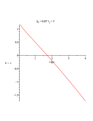
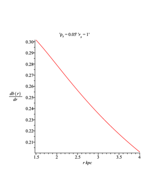
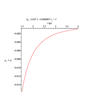
Figure 1: (Left) The throat of the wormhole occurs where $b(r)-r$ cuts the $r$-axis. (Middle) Diagram of the derivative of the shape function of the wormhole. (Right) The variation of the left-hand side of the expression for the null energy condition of matter in the galactic halo is plotted against $r$. We have used geometric units, G=c=1 for choosing the values of $\rho_{s}=0.05$ and $r_{s}=1$.

Regarding these requirements, observe that Eq. (6) shows that the spacetime does not have an event horizon. To check the shape function, we will use a graphical approach by using some typical values of the parameters. Fig. 1 (left panel) shows the following: the throat is located at $r=r_{0}$, where $b(r)-r$ cuts the $r$-axis. Also, for $r>r_{0}$, $b(r)-r<0$, which implies that $b(r)/r<1$, an essential requirement for a shape function. Moreover, $b(r)-r$ is a decreasing function for $r\geq r_{0}$. Therefore, $b^{\prime}(r_{0})<1$, so that the the flare-out condition is satisfied. Fig. 1 (middle panel) also supports this assertion. So all three conditions are satisfied. For the sake of completeness, observe that for the values in Fig. 1, $\rho_{s}=0.05$ and $r_{s}=1$, we obtain $r_{0}=1.7192$ kpc to four decimal places with $b^{\prime}(1.7192)\approx 0.29218$.

Our final task concerning the wormhole structure is to examine the null energy condition. This condition must be violated if the wormhole is to remain open MT88 . Judging from Fig. 1 (right panel), this is indeed the case since $p_{r}+\rho<0$.

For a spacetime to be asymptotically flat, both $f(r)$ and $b(r)/r$ have to approach zero as $r\rightarrow\infty$. The second condition is satisfied, but not the first, as we can see from Eq. (6). So the wormhole cannot be arbitrarily large, which also applies to the halo region. The usual procedure is to cut off the wormhole material at some radial distance and join the solution to an external Schwarzschild spacetime.

It is also useful to calculate the active gravitational mass of the wormhole from the throat, $r_{0}$ (in kpc) up to the radius $R$. This mass is given by

$$M_{active}=4\pi\int_{r_{0}}^{R}\rho r^{2}dr\\ =4\pi\rho_{s}r_{s}^{3}\left[\ln\left(1+\frac{r}{r_{s}}\right)+\frac{1}{\left(1+\frac{r}{r_{s}}\right)}\right]^{R}_{r_{0}}.$$ (9)

Observe that the active gravitational mass $M_{active}$ of the wormhole is positive. This implies that seen from the Earth, we would not be able to distinguish the gravitational nature of a wormhole from that of a compact mass in the galaxy.

3 Equilibrium condition

The generalized Tolman-Oppenheimer-Volkov (TOV) equation is

$$\frac{dp_{r}}{dr}+\frac{\nu^{\prime}}{2}\left(\rho+p_{r}\right)+\frac{2}{r}\left(p_{r}-p_{t}\right)=0.$$ (10)

According to Ponce de León’s suggestion Leon1993 , we rewrite the above TOV equation (10) for the anisotropic mass distribution in the galactic halo, to the following form

$$-\frac{M_{G}\left(\rho+p_{r}\right)}{r^{2}}e^{\frac{\lambda-\nu}{2}}-\frac{dp_{r}}{dr}+\frac{2}{r}\left(p_{t}-p_{r}\right)=0,$$ (11)

where $M_{G}=M_{G}(r)$ is the effective gravitational mass from the throat to some radius $r$ and is given by

$$M_{G}(r)=\frac{1}{2}r^{2}e^{\frac{\nu-\lambda}{2}}\nu^{\prime}.$$ (12)

This expression of mass can be derived from the Tolman-Whittaker formula and the Einstein’s field equations. It is quite natural that the modified TOV equation (11) provides the information of the equilibrium condition for the wormhole subject to gravitational ($F_{g}$) and hydrostatic ($F_{h}$) plus another force due to the anisotropic nature ($F_{a}$) of the matter comprising the wormhole. Hence, for equilibrium the above equation (11) takes the form

$$F_{g}+F_{h}+F_{a}=0,$$ (13)

where,

$$F_{g}=-\frac{\nu^{\prime}}{2}\left(\rho+p_{r}\right)$$ (14)

$$F_{h}=-\frac{dp_{r}}{dr}$$ (15)

$$F_{a}=\frac{2}{r}\left(p_{t}-p_{r}\right)$$ (16)

The profiles of $F_{g}$, $F_{h}$ and $F_{a}$ for the matter distribution of the galactic halo region are shown in Fig. 2. The figure indicates that equilibrium stage can be achieved due to the combined effect of pressure anisotropic, gravitational and hydrostatic forces. It is to be noted that value of $F_{g}$ is too small. The other two plots reside nearly opposite to each other to make the system balanced.

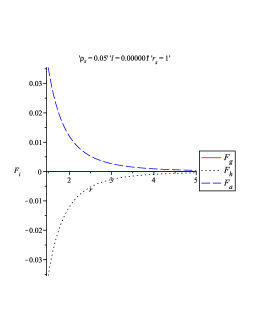
Figure 2: Three different forces acting on fluid elements in static equilibrium is shown against $r$. Value of $F_{g}$ is too small.

4 Scattering of scalar waves in wormhole geometry

The minimally coupled massless wave equation in a wormhole background is given by

$$\qed\Phi=\frac{1}{\sqrt{-g}}\partial_{\mu}[\sqrt{-g}g^{\mu\nu}\partial_{\nu}\Phi]=0.$$ (17)

Note that for simplicity, we are dealing with minimally coupled scalar waves. Since the wormhole spacetime is spherically symmetric, the equation related to scalar field can be solved by separation of variables,

$$\Phi_{l_{0}m}=Y_{l_{0}m}(\theta,\phi)\frac{U_{l_{0}}(r,t)}{r}.$$ (18)

Here $Y_{l_{0}m}(\theta,\phi)$ are the spherical harmonics and $l_{0}$ is the quantum angular momentum.

The possibility of astrophysical observations now provides the motivation for studying the scattering of scalar waves in our wormhole spacetime. Such observations would be important for research on the gravitational radiation, as well as for determining the possible existence of actual physical wormholes.

Using the separable form (18) in (17), one can obtain

$$\left[\frac{1}{\sin\theta}\frac{\partial}{\partial\theta}\sin\theta\frac{\partial}{\partial\theta}+\frac{1}{\sin^{2}\theta}\frac{\partial^{2}}{\partial\phi^{2}}\right]Y_{l_{0}m}=l_{0}(l_{0}+1)Y_{l_{0}m}$$ (19)

and

$$\ddot{U}_{l_{0}}+\frac{\partial^{2}U_{l_{0}}}{\partial{r^{*}}^{2}}=V_{l_{0}}U_{l_{0}},$$ (20)

where the potential $V_{l_{0}}$ is given by

$$V_{l_{0}}=e^{2f}\left[\frac{l_{0}(l_{0}+1)}{r^{2}}-\frac{b^{\prime}r-b}{2r^{3}}+\frac{1}{r}\left(1-\frac{b}{r}\right)f^{\prime}\right].$$ (21)

Here we have used the tortoise coordinate transformation $r^{*}$, i.e.,

$$\frac{\partial}{\partial{r^{*}}}=e^{f}\sqrt{1-\frac{b}{r}}\frac{\partial}{\partial r},$$ (22)

where the dot represents the differentiation with respect to $t$. Actually, $r^{*}$ is the proper distance given by (using $r_{s}=1$)

$$r^{*}=\int_{r_{0}}^{r}\frac{x^{-\frac{l}{2}}dx}{\sqrt{1-\frac{4\pi\rho_{s}\ln(1+x)+\frac{4\pi\rho_{s}}{1+x}}{x}}}.$$ (23)

Since integration cannot be performed in exact analytical form, we find the numerical values of the proper distance $r^{*}$ for given values of radial distance $r$ from the throat radius $r_{0}$, which is shown in Table 1.

Table 1: Values of $r^{*}$ for different r. ($r_{0}=1.7192$, $r_{s}=1$ , $\rho_{s}=.05$)

$r$	$r^{*}$
5	4.9884
10	11.1906
15	16.9754
20	22.5755
25	28.0675
30	33.4974

Observe that characteristics of the potential are determined by the shape and redshift functions of the wormhole.

Assuming the time dependence of the wave to be harmonic, one can write

$$U_{l_{0}}(r,t)=\widehat{U}_{l_{0}}(r,\omega)e^{-i\omega t}.$$ (24)

Using (17) in (20), we get the Schrödinger equation

$$\left[\frac{d^{2}}{d{r^{*}}^{2}}+\omega^{2}-V_{l_{0}}(r)\right]\widehat{U}_{l_{0}}(r,\omega)=0.$$ (25)

Near the throat ($r_{0}\longrightarrow b(r_{0})$), the potential $\approx e^{2f(r_{0})}\left[\frac{l_{0}(l_{0}+1)}{r_{0}^{2}}\right]$, which is finite.

Since the wormhole proposed here is not arbitrarily large, we assume that the wormhole material extends from the throat $r_{0}=1.7192$ kpc to the radius $300$ kpc. For the value of $l=.000001$, note that the magnitude of $V_{l_{0}}$ is negligible at $r=30$ kpc. This means that the solution has the form of a plane wave $\widehat{U}_{l_{0}}\sim e^{\pm i\omega r^{*}}$ at the distance $r=300$ kpc. This result indicates that if a scalar wave passes through the wormhole, the solution would be changed from $e^{\pm i\omega r}$ to $e^{\pm i\omega r^{*}}$. This confirms that the potential affects the scattering of scaler waves.

5 Conclusion

We have shown in this paper that the galactic halo possesses some of the characteristics needed to support a traversable wormhole. The analysis is based on two observational results, the density profile from simulations performed in the $\Lambda$CDM scenario and the observed flat galactic rotation curves. The results should provide sufficient incentives for scientists to seek observational evidence for wormholes, all the more since our study is based on the rotational velocity $v^{\phi}\sim 10^{-3}$ (300 km/s) and a mass of $1.8\times 10^{12}M_{\odot}$ within 300 kpc, making our own galaxy typical enough to be a good candidate. We have briefly studied here balancing of the forces that provides the equilibrium configuration of the system and also proposed a possible detection of such wormholes by studying the scattering of scaler waves.

Appendix 1

We derive the tangential velocity of circular orbits for the line element

$$ds^{2}=-e^{\nu(r)}dt^{2}+e^{\lambda(r)}dr^{2}+r^{2}(d\theta^{2}+sin^{2}\theta\,d\phi^{2}).$$ (26)

The Lagrangian for a test particle is given by

$$2\mathcal{L}=-e^{\nu(r)}\dot{t}^{2}+e^{\lambda(r)}\dot{r}^{2}+r^{2}(\dot{\theta}^{2}+sin^{2}\theta\,\dot{\phi}^{2}),$$ (27)

where the overdot indicates differentiation with respect to the affine parameter $s$. The metric coefficients do not depend explicitly on $t$, $\theta$, or $\phi$. So the Euler-Lagrange equation yields directly the following conserved quantities: the energy $E=-e^{\nu(r)}\dot{t}$, the $\theta$-momentum $L_{\theta}=r^{2}\dot{\theta}$, and the $\phi$-momentum $L_{\phi}=r^{2}{sin}^{2}\theta\,\dot{\phi}$. So the square of the total angular momentum is

$$L^{2}=L_{\theta}^{2}+\left(\frac{L_{\phi}}{sin{\theta}}\right)^{2}=r^{4}(\dot{\theta}^{2}+sin^{2}\theta\,\dot{\phi}^{2}).$$ (28)

With the conserved quantities $E$ and $L$ and the norm of the four-velocity $u^{\mu}u_{\nu}=-1$, the geodesic equation becomes

$$-1=-e^{\nu(r)}\dot{t}^{2}+e^{\lambda(r)}\dot{r}^{2}+r^{2}(\dot{\theta}^{2}+{sin}^{2}\theta\,\dot{\phi}^{2}).$$ (29)

As a result,

$$e^{\nu(r)+\lambda(r)}\dot{r}^{2}+e^{\nu(r)}\left(1+\frac{L^{2}}{r^{2}}\right)=E^{2}$$ (30)

or

$$e^{\lambda(r)}\dot{r}^{2}+1+\frac{L^{2}}{r^{2}}-e^{-\nu(r)}E^{2}=0.$$ (31)

From the equation of motion

$$\dot{r}^{2}+V(r)=0,$$ (32)

we may deduce

$$V(r)=-e^{-\lambda(r)}\left(e^{-\nu(r)}E^{2}-\frac{L^{2}}{r^{2}}-1\right).$$ (33)

However, according to Ref. NSS01 , since we are dealing with circular orbits, it is more convenient to use Eq. (31) and the effective potential

$$V_{eff}=1+\frac{L^{2}}{r^{2}}-e^{-\nu(r)}E^{2}.$$ (34)

Dealing with circular orbits, the following conditions must be satisfied: $\dot{r}=0$, $V_{r}=0$ and $V_{rr}~{}>~{}0$ sC83 . The first condition gives directly

$$E^{2}=e^{\nu(r)}\left(1+\frac{L^{2}}{r^{2}}\right),$$ (35)

and from Eq. (34), the second condition yields

$$\frac{L^{2}}{r^{2}}=\frac{1}{2}r\nu^{\prime}(r)e^{-\nu(r)}E^{2},$$ (36)

or

$$E^{2}=\frac{e^{\nu(r)}}{1-\frac{1}{2}r\nu^{\prime}(r)}$$ (37)

and

$$L^{2}=\frac{\frac{1}{2}r^{3}\nu^{\prime}(r)}{1-\frac{1}{2}r\nu^{\prime}(r)}.$$ (38)

Turning next to the tangential velocity $v^{\phi}$, we have LL75

$$(v^{\phi})^{2}=r^{2}e^{-\nu(r)}\left[\left(\frac{d\theta}{dt}\right)^{2}+{sin}^{2}\theta\left(\frac{d\phi}{dt}\right)^{2}\right]$$

$$=r^{2}e^{-\nu(r)}\left[\left(\frac{d\theta}{ds}\frac{ds}{dt}\right)^{2}+{{sin}^{2}\theta}\left(\frac{d\phi}{ds}\frac{ds}{dt}\right)^{2}\right]$$

$$=r^{2}e^{-\nu(r)}(\dot{\theta}^{2}+{{sin}^{2}\theta}\dot{\phi}^{2})\frac{1}{\dot{t}^{2}}.$$ (39)

By Eq. (28),

$$(v^{\phi})^{2}=\frac{L^{2}\widehat{}}{E^{2}}\frac{1}{r^{2}}e^{\nu(r)}$$ (40)

and by Eq. (36),

$$(v^{\phi})^{2}=\frac{1}{2}r\nu^{\prime}(r).$$ (41)

Integrating, we obtain

$$e^{\nu}=Br^{l},$$

where $B$ is an integration constant and $l=2(v^{\phi})^{2}$.

Now from Eq. (34),

$$V_{eff}(r)_{rr}=\frac{6L^{2}}{r^{4}}-E^{2}e^{-\nu}(\nu^{\prime})^{2}+E^{2}e^{-\nu}v^{\prime\prime}.$$ (42)

Substituting for $E^{2}$, $L^{2}$, and $\nu$, we obtain

$$V_{eff}(r)_{rr}=\frac{2l}{r^{2}}>0,$$

showing the existence of stable orbits.


Appendix 2

The Einstein field equations (in geometrized units $G=c=1$) for the metric (3) are

$$\frac{b^{\prime}(r)}{r^{2}} = 8\pi\rho(r),$$ (43)

$$2\left(1-\frac{b}{r}\right)\frac{f^{\prime}}{r}-\frac{b}{r^{3}} = 8\pi p_{r}(r),$$ (44)

$$\left(1-\frac{b}{r}\right)\left[f^{\prime\prime}+\frac{f^{\prime}}{r}+{f^{\prime}}^{2}-\left\{\frac{b^{\prime}r-b}{2r(r-b)}\right\}\left(f^{\prime}+\frac{1}{r}\right)\right] = 8\pi p_{t}(r).$$ (45)

Using Eqs. (1) and (5), we obtain the following solutions:

$$b(r)=8\pi\rho_{s}r_{s}^{3}\left[\ln\left(1+\frac{r}{r_{s}}\right)+\frac{1}{\left(1+\frac{r}{r_{s}}\right)}\right],$$ (46)

$$8\pi r_{s}^{2}p_{r}=\frac{l}{(\frac{r}{r_{s}})^{2}}\left[1-\frac{8\pi\rho_{s}r_{s}^{2}}{\frac{r}{r_{s}}}\left\{\ln\left(1+\frac{r}{r_{s}}\right)+\frac{1}{\left(1+\frac{r}{r_{s}}\right)}\right\}\right]$$

$$-\frac{8\pi\rho_{s}r_{s}^{2}}{(\frac{r}{r_{s}})^{3}}\left[\ln\left(1+\frac{r}{r_{s}}\right)+\frac{1}{\left(1+\frac{r}{r_{s}}\right)}\right],$$ (47)

$$8\pi r_{s}^{2}p_{t}=\left[1-\frac{8\pi\rho_{s}r_{s}^{2}}{\frac{r}{r_{s}}}\left\{\ln\left(1+\frac{r}{r_{s}}\right)+\frac{1}{\left(1+\frac{r}{r_{s}}\right)}\right\}\right]\times$$

$$\left[\frac{l^{2}}{4(\frac{r}{r_{s}})^{2}}-\left\{\frac{\frac{8\pi\rho_{s}r_{s}^{2}}{\left(1+r/r_{s}\right)^{2}}-\frac{8\pi\rho_{s}r_{s}^{2}}{(r/r_{s})^{2}}\left[\ln\left(1+\frac{r}{r_{s}}\right)+\frac{1}{1+r/r_{s}}\right]}{2\left[1-\frac{8\pi\rho_{s}r_{s}^{2}}{r/r_{s}}\left\{\ln\left(1+\frac{r}{r_{s}}\right)+\frac{1}{1+r/r_{s}}\right\}\right]}\right\}\left\{\frac{l}{2\frac{r}{r_{s}}}+\frac{1}{\frac{r}{r_{s}}}\right\}\right].$$ (48)

References

- (1) M.S. Morris, K.S. Thorne, Am. J. Phys. 56, 395 (1988)
- (2) F.S.N. Lobo, Phys. Rev. D 71, 084011 (2005).
- (3) P.K.F. Kuhfittig, Gen. Rel. Grav. 41, 1485 (2009)
- (4) G. Jungman, M. Kamionkowski, K. Griest, Phys. Rep. 267, 195 (1996)
- (5) E.W. Kolb, M.S. Turner, The Early Universe, Addison Wesley, Redwood City, California (1990)
- (6) S. Fay, Astron. Astrophys. 413, 799 (2004); T. Matos, F.S. Guzman, D. Nunez, Phys. Rev. D 62, 061301 (2000); K.K. Nandi, I. Valitov, N.G. Migranov, Phys. Rev. D 80, 047301 (2009); M. Colpi, S.L. Shapiro, I. Wasserman, Phys. Rev. Lett. 57, 2485 (1986)
- (7) U. Nukamendi, M. Salgado, D. Sudarsky, Phys. Rev. Lett. 84, 3037 (2000); T. Lee, B. Lee, Phys. Rev. D 69, 127502 (2004); F. Rahaman, R. Mondal, M. Kalam, B. Raychaudhuri, Mod. Phys. Lett. A 22, 971 (2007)
- (8) M.K. Mak, T. Harko, Phys. Rev. D 70, 024010 (2004); F. Rahaman, M. Kalam, A. DeBenedictis, A.A. Usmani, S. Ray, Mon. Not. R. Astron. Soc. 389, 27 (2008); K.K. Nandi, A.I. Filippov, F. Rahaman, S. Ray, A.A. Usmani, M. Kalam, A. DeBenedictis, Mon. Not. R. Astron. Soc. 399, 2079 (2009)
- (9) F. Rahaman, P.K.F. Kuhfittig, K. Chakraborty, A.A. Usmani, S. Ray, Gen. Rel. Grav. 44, 905 (2012)
- (10) C.G. Böhmer, T. Harko, F.S.N. Lobo, Astropart. Phys. 29, 386 (2008)
- (11) F. Rahaman et al., Int. J. Theor. Phys [in press], arXiv: 1207.2145[gr-qc], DOI:10.1007/s10773-013-1817-7
- (12) J.F. Navarro et al., Astrophys. J. 462, 563 (1996); J.F. Navarro et al., Astrophys. J. 490, 493 (1997)
- (13) U. Nucamendi, M. Salgado, D. Sudarsky, Phys. Rev. D 63, 125016 (2001)
- (14) J. Ponce de León, Gen. Relativ. Gravit. 25, 1123 (1993)
- (15) S. Chandrasekhar, Mathematical Theory of Black Holes, Oxford, Classic Texts (1983)
- (16) L.D. Landau, E.M. Lifshitz, The Classical Theory of Fields, Oxford, Pergamon Press (1975)