Large unicellular maps in high genus

Abstract

We study the geometry of a random unicellular map which is uniformly distributed on the set of all unicellular maps whose genus size is proportional to the number of edges. We prove that the distance between two uniformly selected vertices of such a map is of order $\log n$ and the diameter is also of order $\log n$ with high probability. We further prove a quantitative version of the result that the map is locally planar with high probability. The main ingredient of the proofs is an exploration procedure which uses a bijection due to Chapuy, Feray and Fusy ([14]).

Keywords: Unicellular maps, high genus maps, hyperbolic, diameter, typical distance, C-permutations.

1 Introduction

A map is an embedding of a finite connected graph on a compact orientable surface viewed up to orientation preserving homeomorphisms such that the complement of the embedding is an union of disjoint topological discs. Loops and multiple edges are allowed and our maps are also rooted, that is, an oriented edge is specified as the root. The connected components of the complement are called faces. The genus of a map is the genus of the surface on which it is embedded. If a map has a single face it is called a unicellular map. On a genus $0$ surface, that is, on the sphere, unicellular maps are classically known as plane (embedded) trees. Thus unicellular maps can be viewed as generalization of a plane tree on a higher genus surface.

Suppose $v$ is the number of vertices in a unicellular map of genus $g$ with $n$ edges. Then Euler’s formula yields

$$v-n=1-2g$$ (1.1)

Observe from eq. 1.1 that the genus of a unicellular map with $n$ edges can be at most $n/2$. We are concerned in this paper with unicellular maps whose genus grows like $\theta n$ for some constant $0<\theta<1/2$. Specifically, we are interested the geometry of a typical element among such maps as $n$ becomes large.

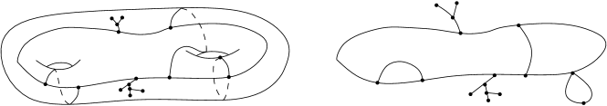
Figure 1: On the left: a unicellular map of genus $2$. On the right: its underlying graph.

Recall that $\mathcal{U}_{g,n}$ denotes the set of unicellular maps of genus $g$ with $n$ edges and let $U_{g,n}$ denote a uniformly picked element from $\mathcal{U}_{g,n}$ for integers $g\geq 0$ and $n\geq 1$. For a graph $G$, let $d^{G}(.,.)$ denote its graph distance metric. Our first main result shows that the distance between two uniformly and independently picked vertices from $U_{g,n}$ is of logarithmic order if $g$ grows like $\theta n$ for some constant $0<\theta<1/2$.

Theorem 1.1.

Let $\{g_{l},n_{l}\}_{l}$ be a sequence in $\mathbb{N}^{2}$ such that $\{g_{l},n_{l}\}\to\{\infty,\infty\}$ and $g_{l}/n_{l}\to\theta$ for some constant $0<\theta<1/2$. Suppose $V_{1}$ and $V_{2}$ are two uniformly and independently picked vertices from $U_{g_{l},n_{l}}$. Then there exists constants $0<\varepsilon<C$ (depending only on $\theta$) such that

• $\mathbb{P}(d^{U_{g_{l},n_{l}}}(V_{1},V_{2})>\varepsilon\log n_{l})\to 1$ as $l\to\infty$.

• $\mathbb{P}(d^{U_{g_{l},n_{l}}}(V_{1},V_{2})>C\log n_{l})<c(n_{l})^{-3}$ for some $c>0$.

We remark here that in the course of the proof of part (i) of Theorem 1.1, a polynomial lower bound on the rate of convergence will be obtained. But since it is far from being sharp and is not much more enlightening, we exclude it from the statement of the Theorem. For part (ii) however, we do provide an upper bound on the rate. Notice that part (ii) enables us to immediately conclude that the diameter of $U_{g_{l},n_{l}}$ is also of order $\log n$ with high probability. For any finite map $G$, let $diam(G)$ denote the diameter of its underlying graph.

Corollary 1.2.

Let $\{g_{l},n_{l}\}_{l}$ be a sequence in $\mathbb{N}^{2}$ such that $\{g_{l},n_{l}\}\to\{\infty,\infty\}$ and $g_{l}/n_{l}\to\theta$ for some constant $0<\theta<1/2$. Then there exists constants $\varepsilon>0,C>0$ such that

$$\mathbb{P}(\varepsilon\log n<diam(U_{g_{l},n_{l}})<C\log n)\to 1$$

as $n\to\infty$.

Proof.

The existence of $\varepsilon>0$ such that $\mathbb{P}(diam(U_{g_{l},n_{l}})>\varepsilon\log n)\to 1$ follows directly from Theorem 1.1 part (i). For the other direction, pick the same constant $C$ as in Theorem 1.1. Let $N$ be the number of pairs of vertices $(v,w)$ in $U_{g_{l},n_{l}}$ where the distance between them is least $C\log n$. From part (ii) of Theorem 1.1, $\mathbb{E}(N)<cn_{l}^{-1}$ for some $c>0$. Hence $\mathbb{E}N$ converges to $0$ as $l\to\infty$. Consequently, $\mathbb{P}(N>0)$ also converges to $0$ which completes the proof. ∎

If the genus is fixed to be $0$, that is in the case of plane trees, the geometry is well understood (see [26] for a nice exposition on this topic.) In particular, it can be shown that the typical distance between two uniformly and independently picked vertices of a uniform random plane tree with $n$ edges is of order $\sqrt{n}$. The diameter of such plane trees is also of order $\sqrt{n}$. These variables when properly rescaled, converge in distribution to appropriate functionals of the Brownian excursion. This characterization stems from the fact that a plane tree can be viewed as a metric space and the metric if rescaled by $\sqrt{n}$ (up to constants) converges in the Gromov-Hausdorff topology (see [20] for precise definitions) to the Brownian continuum random tree (see [2] for more on this.) The Benjamini-Schramm limit in the local topology (see [6, 9] for definitions), of the plane tree as the number of edges grow to infinity is also well understood: the limit is a tree with an infinite spine with critical Galton-Watson trees of geometric$(1/2)$ offspring distribution attached on both sides (see [23] for details.)

Thus Theorem 1.1 depicts that the picture is starkly different if the genus of unicellular maps grow linearly in the number of vertices. The main idea behind the proof of Theorem 1.1 is that locally, $U_{g,n}$ behaves like a supercritical Galton-Watson tree, hence the logarithmic order. We believe that the quantity $d^{U_{g_{l},n_{l}}}(V_{1},V_{2})$ of Theorem 1.1 when rescaled by $\log n$ should converge to a deterministic constant. Further, we also believe that the diameter of $U_{g_{l},n_{l}}$ when rescaled by $\log n$ should also converge to another deterministic constant. This constant obtained from the rescaled limit of the diameter should be different from the constant obtained as a rescaled limit of typical distances. The heuristic behind this extra length of the diameter is the existence of large “bushes” of order $\log n$ on the scheme of the unicellular map (scheme of a unicellular map is obtained by iteratively deleting all the leaves and then erasing the degree $2$ vertices of the map,) a behaviour reminiscent of Erdos-Renyi random graphs (see [13] for more on schemes.)

It is worth mentioning here that unicellular maps have appeared frequently in the field of combinatorics in the past few decades. It is related to representation theory of symmetric group, permutation factorization, matrix integrals computation and also the general theory of enumeration of maps. See the introduction section of [13, 10] for a nice overview and see [25] for connections to other areas of mathematics and references therein.

Recall that a quadrangulation (resp. triangulation) is a map where each face has degree $4$ (resp. $3$). It has been known for some time that distributional limits in the local topology of rooted maps (see [9] for definitions) of uniform triangulations/quadrangulations of the sphere exists and the limiting measure is popularly known as uniform infinite planar triangulation/quadrangulation or UIPT/Q in short (see [6, 3, 24].) Our interest and main motivation for this work is creating hyperbolic analogues of UIPT/Q. It is believed that uniform triangulations/quadrangulations of a surface whose genus is proportional to the number of faces of the map converges in distribution to a hyperbolic analogue of the UIPT/Q if the distributional limit is planar, that is, there are no handles in the limit. A plausible construction of such a limiting hyperbolic random quadrangulation, known as stochastic hyperbolic infinite quadrangulation or SHIQ, can be found in [8]. A half planar version of such hyperbolic maps also arise in [5]. It is worth mentioning here that such limits are expected to hold for any reasonable class of maps and there is nothing special about quadrangulations or triangulations. As is the general strategy in this area, we attempt to attack the problem for quadrangulations using the bijections between labelled unicellular maps and quadrangulations of the same genus (see [15].) Understanding high genus random unicellular maps can be the first step in this direction. Firstly, understanding whether $U_{g,n}$ is locally planar with high probability is a question of interest here.

Tools developed for proving Theorem 1.1 also helps us conclude that locally $U_{g,n}$ is in fact planar with high probability which is our next main result. In fact, we are also able to quantify up to what distance from the root does $U_{g,n}$ remain planar. This will be made precise in the next theorem. A natural question at this point is what is the planar distributional limit of $U_{g,n}$ in the local topology. This is investigated in [4].

We now introduce the notion of local injectivity radius of a map. Since random permutations will play a crucial role in this paper, there will be two notions of cycles floating around: one for cycle decomposition of permutations and the other for maps and graphs. To avoid confusion, we shall refer to a cycle in the context of graphs as a circuit. A circuit in a planar map is a subset of its vertices and edges whose image under the embedding is topologically a loop. A circuit is called contractible if its image under the embedding on the surface can be contracted to a point. A circuit is called non-contractible if it is not contractible.

Definition 1.

The local injectivity radius of a planar map with root vertex $v^{*}$ is the largest $r$ such that the sub-map formed by all the vertices within graph distance $r$ from $v^{*}$ does not contain any non-contractible circuit.

In the world of Riemannian geometry, injectivity radius around a point $p$ on a Riemannian manifold refers to the largest $r$ such that the ball of radius $r$ around $p$ is diffeomorphic to an Euclidean ball via the exponential map. This notion is similar in spirit to what we are seeking in our situation. Notice however that a circuit in a unicellular map is always non-contractible because it has a single face. Hence looking for circuits and looking for non-contractible circuits are equivalent in our situation.

Theorem 1.3.

Let $\{g_{l},n_{l}\}\to\{\infty,\infty\}$ and $g_{l}/n_{l}\to\theta$ for some constant $0<\theta<1/2$ as $l\to\infty$. Let $I_{g_{l},n_{l}}$ denote the local injectivity radius of $U_{g_{l},n_{l}}$. Then there exists a constant $\varepsilon>0$ such that

$$\mathbb{P}\left(I_{g_{l},n_{l}}>\varepsilon\log n_{l}\right)\to 1$$

as $l\to\infty$.

Girth or the circuit of the smallest size of $U_{g,n}$ also deserves some comment. It is possible to conclude via second moment methods that the girth of $U_{g_{l},n_{l}}$ form a tight sequence. This shows that there are small circuits somewhere in the unicellular map, but they are far away from the root with high probability.

The main tool for the proofs is a bijection due to Chapuy, Feray and Fusy ([14]) which gives us a connection between unicellular maps and certain objects called $C$-decorated trees which preserve the underlying graph properties (details in Section 2.1.) This bijection provides us a clear roadway for analyzing the underlying graph of such maps.

From now on fo simplicity, we shall drop the suffix $l$ in $\{g_{l},n_{l}\}$, and assume $g$ as a function of $n$ such that $g\to\infty$ as $n\to\infty$ and $g/n\to\theta$ where $0<\theta<1/2$. The proofs that follow will not be affected by such simplification as one might check. For any sequence $\{a_{n}\}$ and $\{b_{n}\}$ of positive integers, $a_{n}\sim b_{n}$ means $a_{n}/b_{n}\to 1$. Further $a_{n}=o(b_{n})$ means that $a_{n}/b_{n}\to 0$ as $n\to\infty$ and $a_{n}=O(b_{n})$ means that there exists a universal constant $C>0$ such that $|a_{n}|<C|b_{n}|$. Finally $a_{n}\asymp b_{n}$ means there exists positive universal constants $c_{1},c_{2}$ such that $c_{1}b_{n}<a_{n}<c_{2}b_{n}$. In what follows, the constants might vary from step to step but for simplicity, we shall denote the constants which we do not need anywhere else by $c$. For a finite set $X$, $|X|$ denotes the cardinality of $X$.

Overview of the paper:

In Section 2 we gather some useful preliminary results we need. Proofs and references of some of the results in Section 2 are provided in appendices A and B. An overview of the strategy of the proofs of Theorems 1.1 and 1.3 is given in Section 3. Part (ii) of Theorem 1.1 along with Theorem 1.3 is proved in Section 4. Part (i) of Theorem 1.1 is proved in Section 5.

Acknowledgements:

The author is indebted to Omer Angel for carefully reading the manuscript and providing innumerable suggestions to make the paper more readable. The author would also like to thank Guillaume Chapuy, Nicolas Curien, Asaf Nachmias, Bálázs Ráth and Daniel Valesin for several stimulating discussions. The author also thanks the anonymous referee for several useful comments.

2 Preliminaries

In this section, we gather some useful results which we shall need.

2.1 The bijection

Chapuy, Féray and Fusy in ([14]) describes a bijection between unicellular maps and certain objects called $C$-decorated trees. The bijection describes a way to obtain the underlying graph of $U_{g,n}$ by simply gluing together vertices of a plane tree in an appropriate way. This description gives us a simple model to analyze because plane trees are well understood. In this section we describe the bijection in [14] and define an even simpler model called marked trees. The model of marked trees will contain all the information about the underlying graph of $U_{g,n}$.

For a graph $G$, let $V(G)$ denote the collection of vertices and $E(G)$ denote the collection of edges of $G$. The subgraph induced by a subset $V^{\prime}\subseteq V(G)$ of vertices is a graph $(V^{\prime},E^{\prime})$ where $E^{\prime}\subseteq E(G)$ and for every edge $e\in E^{\prime}$, both the vertices incident to $e$ is in $V^{\prime}$.

A permutation of order $n$ is a bijective map $\sigma:\{1,2,\ldots,n\}\to\{1,2,\ldots,n\}$. As is classically known, $\sigma$ can be written as a composition of disjoint cycles. Length of a cycle is the number of elements in the cycle. The cycle type of a permutation is an unordered list of the lengths of the cycles in the cycle decomposition of the permutation. A cycle-signed permutation of order $n$ is a permutation of order $n$ where each cycle in its cycle decomposition carries a sign, either $+$ or $-$.

Definition 2 ([14]).

A $C$-permutation of order $n$ is a cycle-signed permutation $\sigma$ of order $n$ such that each cycle of $\sigma$ in its cycle decomposition has odd length. The genus of $\sigma$ is defined to be $(n-N)/2$ where $N$ is the number of cycles in the cycle decomposition of $\sigma$.

Definition 3 ([14]).

A $C$-decorated tree on $n$ edges is the pair $(t,\sigma)$ where $t$ is a rooted plane tree with $n$ edges and $\sigma$ is a $C$-permutation of order $n+1$. The genus of $(t,\sigma)$ is the genus of $\sigma$.

The set of all $C$-decorated trees of genus $g$ is denoted by $\mathcal{C}_{g,n}$. One can canonically order and number the vertices of $t$ from $1$ to $n+1$. Hence in a $C$-decorated tree $(t,\sigma)$, the permutation $\sigma$ can be seen as a permutation on the vertices of the tree $t$. To obtain the underlying graph of a $C$-decorated tree $(t,\sigma)$, any pair of vertices $x,y$ whose numbers are in the same cycle of $\sigma$ are glued together (note that this might create loops and multiple edges.) The underlying graph of $(t,\sigma)$ is the vertex rooted graph obtained from $(t,\sigma)$ after this gluing procedure. So there are $N$ vertices of the underlying graph of $(t,\sigma)$, each correspond to a cycle of $\sigma$ (see Figure 2). By Euler’s formula, if the underlying graph of $(t,\sigma)$ is embedded in a surface such that there is only one face, then the underlying surface must have genus $g$ given by $N=n+1-2g$.

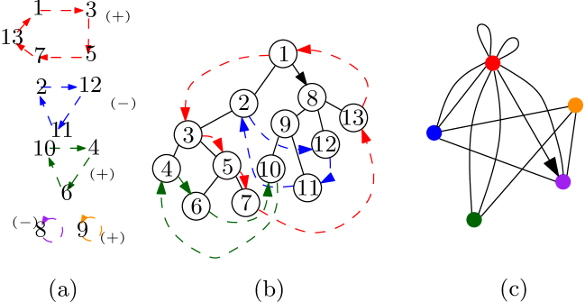
Figure 2: An illustration of a $C$-decorated tree. (a) A $C$-permutation $\sigma$ where each cycle is marked with a different color. (b) A plane tree $t$ with the vertices in the same cycle of $\sigma$ joined by an arrow of the same color as the cycle. Note that vertices numbered $8$ and $9$ are fixed points in the $C$-permutation. (c) The underlying graph of the $C$-decorated tree $(t,\sigma)$. The root vertex is circled.

For a set $\mathcal{A}$, let $k\mathcal{A}$ denote $k$ distinct copies of $\mathcal{A}$. Recall that underlying graph of a unicellular map is the vertex rooted graph whose embedding is the map.

Theorem 2.1.

(Chapuy, Féray, Fusy [14]) There exists a bijection

$$2^{n+1}\mathcal{U}_{g,n}\longleftrightarrow\mathcal{C}_{g,n}.$$

Moreover, the bijection preserves the underlying graph.

As promised, we shall now introduce a further simplified model which we call marked tree to analyze the underlying graph of $C$-decorated trees. Let $\mathcal{P}$ denote the set of ordered $N$-tuple of odd positive integers which add up to $n+1$.

Definition 4.

A marked tree with $n$ edges corresponding to an $N$-tuple $\lambda=(\lambda_{1},\ldots,\lambda_{N})\in\mathcal{P}$ is a pair $(t,m)$ such that $t\in\mathcal{U}_{0,n}$ and $m:V(t)\to\mathbb{N}$ is a function which takes the value $i$ for exactly $\lambda_{i}$ vertices of $t$ for all $i=1,\ldots,N$. The underlying graph of $(t,m)$ is the rooted graph obtained when we merge together all the vertices of $t$ with the same mark.

Given a $\lambda$, let $\mathcal{T}_{\lambda}$ be the set of marked trees corresponding to $\lambda$ and let $T_{\lambda}$ be a uniformly picked element from it. Now pick $\lambda$ from $\mathcal{P}$ according to the following distribution

$$\mathbb{P}\left(\lambda=(\lambda_{1},\lambda_{2},\ldots,\lambda_{N})\right)=\frac{\prod_{i=1}^{N}\lambda_{i}^{-1}}{Z}$$ (2.1)

where $Z=\sum_{\lambda\in\mathcal{P}}(\prod_{i=1}^{N}\lambda_{i}^{-1})$.

Proposition 2.2.

Choose $\lambda$ according to the distribution given by (2.1). Then the underlying graph of $U_{g,n}$ and $T_{\lambda}$ has the same distribution.

Proof.

First observe that it is enough to show the following sequence of bijections

$$2^{N}\bigcup_{\lambda=(\lambda_{1},\ldots,\lambda_{N})\in\mathcal{P}}\prod_{i=1}^{N}(\lambda_{i}-1)!\mathcal{T}_{\lambda}(n)\stackrel{{\scriptstyle\Psi}}{{\longleftrightarrow}}N!\mathcal{C}_{g,n}\stackrel{{\scriptstyle\Phi}}{{\longleftrightarrow}}2^{n+1}N!\mathcal{U}_{g,n}$$

where $\Phi$ and $\Psi$ are bijections which preserve the underlying graph. This is because for each $\lambda\in\mathcal{P}$, it is easy to see that the number of elements in $\prod_{i}(\lambda_{i}-1)!\mathcal{T}_{\lambda}(n)$ is $(n+1)!\prod_{i=1}^{N}\lambda_{i}^{-1}$ and given a $\lambda$, the underlying graph of an uniform element of $\prod_{i}(\lambda_{i}-1)!\mathcal{T}_{\lambda}(n)$ and ${T}_{\lambda}(n)$ has the same distribution.

Now the existence of bijection $\Phi$ which also preserves the underlying graph is guaranteed from Theorem 2.1. For $\Psi$, observe that the factor $\prod_{i=1}^{N}(\lambda_{i}-1)!$ comes from the ordering of the elements within the cycle of $C$-permutations and the factor $2^{N}$ comes from the signs associated with each cycle of the $C$-permutations. The factor $N!$ comes from all possible ordering each cycle type of a $C$-permutation which is taken into account in the marked trees but not $C$-permutations. The details are safely left to the reader. ∎

Because of Lemma 2.2 it is enough to look at the underlying graph of ${T}_{\lambda}(n)$ to prove the Theorems stated in Section 1 where $\lambda$ is chosen according to the distribution given by (2.1). Our strategy is to show that a typical $\lambda$ satisfies some “nice” conditions (which we will call condition $(A)$ later), condition on such a $\lambda$ satisfying those conditions and then work with ${T}_{\lambda}(n)$.

Recall $N=n+1-2g$. Since $g/n\to\theta$ where $0<\theta<1/2$, $n/N\to(1-2\theta)^{-1}$. Denote $\alpha=(1-2\theta)^{-1}$. Clearly $\alpha>1$. The reader should bear in mind that $\alpha$ will remain in the background throughout the rest of the paper.

2.2 Typical $\lambda$

Recall the definition of $\mathcal{P}$ from Section 2.1. Suppose $C_{0},C_{1},C_{2},d_{1},d_{2}$ are some positive constants which we will fix later. We say that an element in $\lambda=(\lambda_{1},\lambda_{2},\ldots\lambda_{N})\in\mathcal{P}$ satisfies condition $(A)$ if it satisfies

• $\lambda_{\max}<C_{0}\log n$ where $\lambda_{\max}$ is the maximum in the set $\{\lambda_{1},\lambda_{2},\ldots\lambda_{N}\}$.

• $C_{1}n<\sum_{i=1}^{N}\lambda_{i}^{2}<\sum_{i=1}^{N}\lambda_{i}^{3}<C_{2}n$.

• $d_{1}n<|i:\lambda_{i}=1|<d_{2}n$

The following Lemma ensures that $\lambda$ satisfies condition $(A)$ with high probability for appropriate choice of the constants. The proof is provided in appendix A

Lemma 2.3.

Suppose $\lambda$ is chosen according to the distribution given by (2.1). Then there exists constants $C_{0},C_{1},C_{2},d_{1},d_{2}$ depending only upon $\alpha$ such that condition $(A)$ holds with probability at least $1-cn^{-3}$ for some constant $c>0$.

Now we state a Lemma which will be useful later. Given a $\lambda$, we shall denote by $\mathbb{P}_{\lambda}$ the conditional measure induced by $T_{\lambda}$.

Lemma 2.4.

Fix a tree $t\in\mathcal{U}_{0,n}$ and a $\lambda\in\mathcal{P}$ satisfying condition $(A)$. Fix $\mathcal{I}\subset\{1,2,\ldots,N\}$ such that $|\mathcal{I}|<n^{3/4}$. Condition on the event $\mathcal{E}$ that the plane tree of ${T}_{\lambda}(n)$ is $t$ and $S$ is the set of all the vertices in $t$ whose mark belong to $\mathcal{I}$ where $S$ is some fixed subset of $V(t)$ ($S$ is chosen so that $\mathcal{E}$ has non-zero probability.) Let $\{v,w,z\}\subset V(t)\setminus S$ be any set of three distinct vertices in $t$ and $i\notin\mathcal{I}$. Then

$$\mathbb{P}_{\lambda}(m(v)=i|\mathcal{E}) \sim\lambda_{i}/n$$ (2.2)

$$\mathbb{P}_{\lambda}(m(v)=m(w)|\mathcal{E}) \asymp n^{-1}$$ (2.3)

$$\mathbb{P}_{\lambda}(m(v)=m(w)=m(z)|\mathcal{E}) \asymp n^{-2}$$ (2.4)

Proof.

Notice that $|S|<C_{0}n^{3/4}\log n$ because of part (i) of condition $(A)$. The proof of (2.2) follows from the fact that

$$\mathbb{P}_{\lambda}(m(v)=i|\mathcal{E})=\frac{(n-|S|-1)!\lambda_{i}!}{(n-|S|)!(\lambda_{i}-1)!}=\frac{\lambda_{i}}{n-|S|}\sim\lambda_{i}/n$$

since $|S|<C_{0}n^{3/4}\log n$.

Now we move on to prove (2.3). Conditioned on $S,t$ the probability that $v$ and $w$ have the same mark $j\notin\mathcal{I}$ with $\lambda_{j}\geq 3$ is

$$\frac{(n-|S|-2)!\lambda_{j}!}{(n-|S|)!(\lambda_{j}-2)!}\sim\frac{\lambda_{j}(\lambda_{j}-1)}{n^{2}}$$

All we need to prove is $\sum_{j\notin\mathcal{I}}\lambda_{j}(\lambda_{j}-1)\asymp n$ which is clear from part (ii) of condition $(A)$ and the fact that $|\mathcal{I}|<n^{3/4}$.

Proof of eq. 2.4 is very similar to that of eq. 2.3 and is left to the reader. ∎

2.3 Large deviation estimates on random trees

2.3.1 Galton-Watson trees

A Galton-Watson tree, roughly speaking, is the family tree of a Galton-Watson process which is also sometimes referred to as a branching process in the literature. These are well studied in the past and goes far back to the work of Harris ([21]). A fine comprehensive coverage about branching processes can be found in [7]. Given a Galton-Watson tree, we denote by $\xi$ the offspring distribution. Let $\mathbb{P}(\xi=k)=p_{k}$ for $k\geq 1$. Let $Z_{r}$ be the number of vertices at generation $r$ of the tree. We shall also assume

• $p_{0}+p_{1}<1$

• $\mathbb{E}(e^{\lambda\xi})<\infty$ for small enough $\lambda>0$.

We need the following lower deviation estimate. The proof essentially follows from a result in [7] and is provided in appendix B.

Lemma 2.5.

Suppose $\mathbb{E}\xi=\mu>1$ and the distribution of $\xi$ satisfies the assumptions as above. For any constant $\gamma$ such that $1<\gamma<\mu$, for all $r\geq 1$

$$\mathbb{P}(Z_{r}\leq\gamma^{r})<c\exp(-c^{\prime}r)+\mathbb{P}(Z_{r}=0)$$

for some positive constants $c,c^{\prime}$.

2.3.2 Random plane trees

A random plane tree with $n$ edges is a uniformly picked ordered tree with $n$ edges (see [26] for a formal treatment.) In other words a random plane tree with $n$ edges is nothing but $U_{0,n}$ as per our notation. We shall need the following large deviation result for the lower bounds and upper bounds on the diameter of $U_{0,n}$. This follows from Theorem $1.2$ of [1] and the discussion in Section $1.1$ of [1].

Lemma 2.6.

For any $x>0$,

• $P(Diam(U_{0,n})\leq x)<c\exp(-c_{1}(n-2)/x^{2})$

• $P(Diam(U_{0,n})>x)<c\exp(-c_{1}x^{2}/n)$

where $c>0$ and $c_{1}>0$ are constants.

We shall also need some estimate of local volume growth in random plane trees. For this purpose, let us define for an integer $r\geq 1$,

$$M_{r}=\max_{v\in V(U_{0,n})}|B_{r}(v)|$$

where $B_{r}(v)$ denotes the ball of radius $r$ around $v$ in the graph distance metric of $U_{0,n}$. In other words, $M_{r}$ is the maximum over $v$ of the volume of the ball of radius $r$ around a vertex $v$ in $U_{0,n}$. It is well known that typically, the ball of radius $r$ in $U_{0,n}$ grows like $r^{2}$. The following Lemma states that $M_{r}$ is not much larger than $r^{2}$ with high probability. Proof is provided in appendix B.

Lemma 2.7.

Fix $j\geq 1$ and $r=r(n)$ is a sequence of integers such that $1\leq r(n)\leq n$. Then there exists a constant $c>0$ such that

$$\mathbb{P}(M_{r}>r^{2}\log^{2}n)<\exp(-c\log^{2}n)$$

3 Proof outline

In this section we describe the heuristics of the proofs of Theorems 1.1 and 1.3.

Let us describe an exploration process on a given marked tree starting from any vertex $v$ in the plane tree. This process will describe an increasing sequence of subsets of vertices which we will call the set of revealed vertices. In the first step, we reveal all the vertices with the same mark as $v$. Then we explore the set of revealed vertices one by one. At each step when we explore a vertex, we reveal all its neighbours and also reveal all the vertices which share a mark with one of the neighbours. If a neighbour has already been revealed, we ignore it. We then explore the unexplored vertices and continue.

We can associate a branching process with this exploration process where the number of vertices revealed while exploring a vertex can be thought of as the offsprings of the vertex. It is well known that the degree of any uniformly picked vertex in $U_{0,n}$ is roughly distributed as a geometric$(1/2)$ variable and we can expect such behaviour of the degree as long as the number of vertices revealed by the exploration is small compared to the size of the tree. Now the expected number of vertices with the same mark as a vertex is roughly a constant strictly larger than $1$ because of part (ii) of condition $(A)$. Hence the associated branching process will have expected number of offsprings a constant which is strictly larger than $1$. Thus we can stochastically dominate this branching process both from above and below by supercritical Galton-Watson processes which will account for the logarithmic order of typical distances.

Once we have such a domination, observe that the vertices at distance at most $r$ from the root in the underlying graph of the marked tree is approximately the vertices in the ball of radius $r$ around the root in a supercritical Galton-Watson tree. Hence by virtue of the fact that supercritical Galton-Watson trees have roughly exponential growth, we can conclude that the number of vertices at a distance at most $\varepsilon\log n$ from the root in the underlying graph of the marked tree is $\ll\sqrt{n}$ if $\varepsilon>0$ is small enough. Hence note that to have a circuit within distance $\varepsilon\log n$ in the underlying graph of the marked tree, two of the vertices which are revealed within $\ll\sqrt{n}$ many steps must be close in the plane tree. But observe that the distribution of the revealed vertices is roughly a uniform sample from the set of vertices in the tree up to the step when at most roughly $\sqrt{n}$ many vertices are revealed. Hence the probability of revealing two vertices which are close in the plane tree up to roughly $\sqrt{n}$ many steps is small because of the birthday paradox argument. This argument shows that the local injectivity radius is at least $\varepsilon\log n$ for some small enough $\varepsilon>0$.

The rest of the paper is the exercise of making these heuristics precise.

4 Lower Bound and Injectivity radius

Recall condition $(A)$ as described in the begininning of Section 2.2. Pick a $\lambda$ satisfying condition $(A)$. Recall that ${T}_{\lambda}(n)$ denotes a uniformly picked element from $\mathcal{T}_{\lambda}(n)$. Throughout this section we shall fix a $\lambda$ satisfying condition $(A)$ and work with ${T}_{\lambda}(n)$. Also recall that ${T}_{\lambda}(n)=(U_{0,n},M)$ where $U_{0,n}$ is a uniformly picked plane tree with $n$ edges and $M$ is a uniformly picked marking function corresponding to $\lambda$ which is independent of $U_{0,n}$. Let $d_{\lambda}(.,.)$ denote the graph distance metric in the underlying graph of ${T}_{\lambda}(n)$. In this section we prove the following Theorem.

Theorem 4.1.

Fix a $\lambda$ satisfying condition $(A)$. Suppose $x$ and $y$ are two uniformly and independently picked numbers from $\{1,2,\ldots,N\}$ and $V_{x}$ and $V_{y}$ are the vertices in the underlying graph of ${T}_{\lambda}(n)$ corresponding to the marks $x$ and $y$ respectively. Then there exists a constant $\varepsilon>0$ such that

$$\mathbb{P}_{\lambda}(d_{\lambda}(V_{x},V_{y})<\varepsilon\log n)\to 0$$

as $n\to\infty$.

Proof of Theorem 1.1 part (i).

Follows from Theorem 4.1 along with Propositions 2.2 and 2.3. ∎

As a by-product of the proof of Theorem 4.1, we also obtain the proof of Theorem 1.3 in this section.

Note that for any finite graph, if the volume growth around a typical vertex is small, then the distance between two typical vertices is large. Thus to prove Theorem 4.1, we aim to prove an upper bound on volume growth around a typical vertex. Note that with high probability the maximum degree in $U_{0,n}$ is logarithmic and $\lambda_{\max}$ is also logarithmic (via condition $(A)$ part (i) and Lemma 2.6.) Hence it is easy to see using the idea described in Section 3 that the typical distance is at least $\varepsilon\log n/\log\log n$ with high probability if $\varepsilon>0$ is small enough. This is enough, as is heuristically explained in Section 3, to ensure that the injectivity radius of $U_{g}(n)$ is at least $\varepsilon\log n/\log\log n$ with high probability for small enough constant $\varepsilon>0$. The rest of this section is devoted to the task of getting rid of the $\log\log n$ factor. This is done by ensuring that while performing the exploration process for reasonably small number of steps, we do not reveal vertices of high degree with high probability.

Given a marked tree $(t,m)$, we shall define a nested sequence $R_{0}\subseteq R_{1}\subseteq R_{2}\subseteq\ldots$ of subgraphs of $(t,m)$ where $R_{k}$ will be the called the subgraph revealed and the vertices in $R_{k}$ will be called the vertices revealed at the $k$th step of the exploration process. We will also think of the number of steps as the amount of time the exploration process has evolved. There will be two states of the vertices of $R_{k}$: active and neutral. Along with $\{R_{k}\}$, we will define another nested sequence $E_{0}\subseteq E_{1}\subseteq E_{2}\subseteq\ldots$. In the first step, $R_{0}=E_{0}$ will be a set of vertices with the same mark and hence $E_{0}$ will correspond to a single vertex in the underlying graph of $(t,m)$. The subgraph of the underlying graph of $(t,m)$ formed by gluing together vertices with the same mark in $E_{r}$ will be the ball of radius $r$ around the vertex corresponding to $E_{0}$ in the underlying graph of $(t,m)$. The process will have rounds and during round $i$, we shall reveal the vertices which correspond to vertices at distance exactly $i$ from the vertex corresponding to $E_{0}$ in the underlying graph of $(t,m)$. Define $\tau_{0}=0$ and we now define $\tau_{r}$ which will denote the time of completion of the $r$th round for $r\geq 1$. Let $N_{r}=E_{r}\setminus E_{r-1}$. Inductively, having defined $N_{r}$, we continue to explore every vertex in $N_{r}$ in some predetermined order and $\tau_{r+1}$ is the step when we finish exploring $N_{r}$. For a vertex $v$, $mark(v)$ denotes the set of marked vertices with the same mark as that of $v$. For a vertex set $S$, $mark(S)=\cup_{v\in S}mark(v)$. We now give a rigorous algorithm for the exploration process.

Exploration process I

• Starting rule: Pick a number $x$ uniformly at random from the set of marks $\{1,2,\ldots,N\}$ and let $E_{0}=R_{0}=mark(x)$. Declare all the vertices in $mark(x)$ to be active. Also set $\tau_{0}=0$.

• Growth rule:

  1. For some $r\geq 1$, suppose we have defined the nested subset of vertices of $E_{0}\subseteq\ldots\subseteq E_{r}$ such that $N_{r}:=E_{r}\setminus E_{r-1}$ is the set of active vertices in $E_{r}$. Suppose we have defined the increasing sequence of times $\tau_{0}\leq\ldots\leq\tau_{r}$ and the nested sequence of subgraphs $R_{0}\subseteq R_{1}\subseteq\ldots\subseteq R_{\tau_{r}}$ such that $R_{\tau_{r}}=E_{r}$. The number $r$ denotes the number of rounds completed in the exploration process at time $\tau_{r}$.

  2. Order the vertices of $N_{r}$ in some arbitrary order. Now we explore the first vertex $v$ in the ordering of $N_{r}$. Let $S_{v}$ denote all the neighbours of $v$ in $t$ which do not belong to $R_{\tau_{r}}$. Suppose $S_{v}$ has $l$ vertices $\{v_{1},v_{2},\ldots,v_{l}\}$ which are ordered in an arbitrary way. For $1\leq j\leq l$, at step $\tau_{r}+j$, define $R_{\tau_{r}+j}$ to be the subgraph induced by $V(R_{\tau_{r}+j-1})\cup mark(v_{j})$. At step $\tau_{r}+l$ we finish exploring $v$. Define all the vertices in $R_{\tau_{r}+l}\setminus R_{\tau_{r}}$ to be active and declare $v$ to be neutral. Then we move on to the next vertex in $N_{r}$ and continue.

  3. Suppose we have finished exploring a vertex of $N_{r}$ in step $k$ and obtained $R_{k}$. If there are no more vertices left in $N_{r}$, define $k=\tau_{r+1}$ and $E_{r+1}=R_{\tau_{r+1}}$. Declare round $r+1$ is completed and go to step $1$.

  4. Otherwise, we move on to the next vertex $v^{\prime}$ in $N_{r}$ according to the predescribed order. Let $S_{v^{\prime}}=\{v_{1},v_{2},\ldots,v_{l^{\prime}}\}$ be the neighbours of $v^{\prime}$ which do not belong to $R_{k}$. For $1\leq j\leq l^{\prime}$, at step $k+j$, define $R_{k+j}$ to be the subgraph induced by $V(R_{k+j-1})\cup mark(v_{j})$. Define all the vertices in $R_{k+l^{\prime}}\setminus R_{k}$ to be active and declare $v^{\prime}$ to be neutral. Now go back to step $3$.

• Threshold rule: We stop if the number of steps exceeds $n^{1/10}$ or the number of rounds exceeds $\log n$. Let $\delta$ be the step number when we stop the exploration process.

Recall that $V_{x}$ denotes the vertex in the underlying graph of ${T}_{\lambda}(n)$ corresponding to the mark $x$. The following proposition is clear from the description of the exploration process and is left to the reader to verify.

Proposition 4.2.

For every $j\geq 1$, all the vertices with the same mark in $E_{j}\setminus E_{j-1}$ when glued together form all the vertices at a distance exactly $j$ from $V_{x}$ in the underlying graph of $(t,m)$.

In step $0$, define $mark(x)$ to be the seeds revealed in step $0$. At any step, if we reveal $mark(z)$ for some vertex $z$, then $mark(z)\setminus z$ is called the seeds revealed at that step. The nomenclature seed comes from the fact that a seed gives rise to a new connected component in the revealed subgraph unless it is a neighbour of one of the revealed subgraph components. However we shall see that the probability of the latter event is small and typically every connected component has one unique seed from which it “starts to grow”.

Now suppose we perform the exploration process on ${T}_{\lambda}(n)=(U_{0,n},M)$ where recall that $M$ is a uniformly random marking function which is compatible with $\lambda$ on the set of vertices of $U_{0,n}$ and is independent of the tree $U_{0,n}$. Let $\mathcal{F}_{k}$ be the sigma field generated by $R_{0},R_{1},R_{2},\ldots,R_{k}$.

The aim is to control the growth of $R_{k}$ and to that end, we need to control the size of $mark(S_{v})$ while exploring the vertex $v$ conditioned up to what we have revealed up to the previous step. It turns out that it will be more convenient to condition on a subtree which is closely related to the connected tree spanned by the vertices revealed.

               

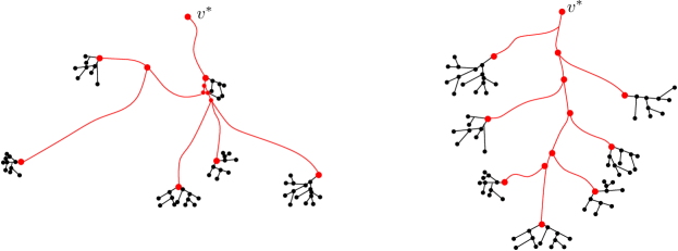
Figure 3: The web is denoted by the red paths. On the left: a general web structure. Apriori the web structure might be very complicated. Many paths in the web might pass through the same vertex as is depicted here. On the right: A typical web structure

Definition 5.

The web corresponding to $R_{k}$ is defined to be the union of the unique paths joining the root vertex $v^{*}$ and the vertices closest to $v^{*}$ in each of the connected components of $R_{k}$ including the vertices at which the paths intersect $R_{k}$. The web corresponding to $R_{k}$ is denoted by $P_{R_{k}}$.

As mentioned before, the idea is to condition on the web. Observe that after removing the web from $U_{0,n}$ at any step, we are left with a uniformly distributed forest with appropriate number of edges and trees. What stands in our way is that in general the web corresponding to a subtree might be very complicated (see Figure 3). The paths joining the root and several components might “go through” the same component. Hence conditioned on the web, a vertex might apriori have arbitrarily many of its neighbours belonging to the web. To show that this does not happen with high probability we need the following definitions.

For any vertex $u$ in $t$, the ancestors of $u$ are the vertices in $t$ along the unique path joining $u$ and the root vertex $v^{*}$. For any two vertices $u,v$ in $t$ let $u\wedge v$ denote the common ancestor of $u$ and $v$ which is farthest from the root vertex $v^{*}$ in $t$. Let

$$C(u,v)=d^{t}(u\wedge v,\{u,v,v^{*}\})$$

A pair of vertices $(u,v)$ is called a bad pair if $C(u,v)<\log^{2}n$ (see Figure 4.)

                                 

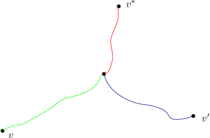
Figure 4: $v^{*}$ denotes the root vertex. $(v,v^{\prime})$ is a bad pair if either of red, green or blue part has at most $\log^{2}n$ many vertices.

Recall that we reveal some set of seeds (possibly empty) at each step of the exploration process. Suppose we uniformly order the seeds revealed at each step and then concatenate them in the order in which they are revealed. More formally, Let $(s_{i_{0}},s_{i_{1}},\ldots,s_{i_{k_{i}}})$ be the set of seeds revealed in step $i$ ordered in uniform random order. Let $S=(s_{1_{0}},s_{1_{1}},\ldots,s_{1_{k_{1}}},\ldots,s_{\delta_{1}},\ldots,s_{\delta_{k_{\delta}}})$. To simplify notation, let us denote $S=(S_{0},S_{1},\ldots,S_{\delta^{\prime}})$ where $\delta^{\prime}+1$ counts the number of seeds revealed up to step $\delta$. The reason for such ordering is technical and will be clearer later in the proof of Lemma 4.7.

Lemma 4.3.

If $S$ does not contain a bad pair then each connected component of $R_{\delta}$ contains an unique seed and the web $P_{R_{\delta}}$ intersects each connected component of $R_{\delta}$ at most at one vertex.

Remark 4.4.

In Lemma 4.9, we shall prove that the probability of $S$ containing a bad pair goes to $0$ as $n\to\infty$. This and Lemma 4.3 shows that for large $n$, the typical structure of the web is like the right hand figure of Figure 3.

Proof.

Clearly, every connected component of $R_{\delta}$ must contain at least one seed. Also note that every connected component of $R_{\delta}$ has diameter at most $2\log n$ because of the threshold rule. Since the distance between any pair of seeds in $R_{\delta}$ is at least $\log^{2}n$ if $S$ do not contain a bad pair, each component must contain a unique seed.

Suppose at any arbitrary step there is a connected component $C$ which intersects the web in more than two vertices. Then there must exist a component $C^{\prime}$ such that the path of the web joining the root and $C^{\prime}$ intersects $C$ in more than one vertex. This implies that the (unique) seeds of $C$ and $C^{\prime}$ form a bad pair since the diameter of both $C$ and $C^{\prime}$ are at most $2\log n$. ∎

Now we want to prove that with high probability, $S$ do not contain a bad pair. Observe that the distribution of the set of seeds revealed is very close to a uniformly sampled set of vertices without replacement from the set of vertices of the tree as long as $R_{\delta}\ll\sqrt{n}$, because of the same effect as the birthday paradox. We quantify this statement and further show that an i.i.d. sample of size $\delta^{\prime}$ from the set of vertices do not contain a bad pair with high probability.

We first show that the cardinality of the set $R_{\delta}$ cannot be too large with high probability.

Lemma 4.5.

$R_{\delta}=O(n^{1/10}\log n)$

Proof.

At each step at most $\lambda_{\max}$ many vertices are revealed and $\lambda_{\max}=O(\log n)$ via condition $(A)$. ∎

Given $S$, let $\widetilde{S}=\{\widetilde{S}_{0},\widetilde{S}_{1},\ldots,\widetilde{S}_{\delta^{\prime}}\}$ be an i.i.d. sample of uniformly picked vertices from $U_{0,n}$. First we need the following technical Lemma.

Lemma 4.6.

Suppose $a=a(n)$ and $b=b(n)$ are sequences of positive integers such that $(a+b)^{2}=o(n)$. Then for large enough $n$,

$$n^{b}\left|\frac{1}{b!}\dbinom{n-a}{b}^{-1}-\frac{1}{n^{b}}\right|<4\left(\frac{(a+b)b}{n}\right)$$

Proof.

Observe that

$$\frac{1}{b!}\dbinom{n-a}{b}^{-1} =\frac{1}{(n-a-b+1)\ldots(n-a)}$$

$$=\frac{1}{n^{b}}\prod_{j=1}^{b}\left(1+\frac{a+b-j}{n-(a+b-j)}\right)$$ (4.1)

$$<\frac{1}{n^{b}}\prod_{j=1}^{b}(1+2(a+b)/n))$$

$$<\frac{1}{n^{b}}\exp\left(\frac{2(a+b)b}{n}\right)$$

$$=\frac{1}{n^{b}}\left(1+\frac{2(a+b)b}{n}+o\left(\frac{(a+b)b}{n}\right)\right)$$

$$<\frac{1}{n^{b}}\left(1+4\left(\frac{(a+b)b}{n}\right)\right)$$

where the third inequality follows because $n-(a+b)>n/2$ for large enough $n$ and $a+b-j<a+b$. The second last equality follows since $b(a+b)=o(n)$ via the hypothesis. The other direction follows from the fact that the expression in the right hand side of eq. 4.1 is larger than $1/n^{b}$. ∎

For random vectors $X,Y$ let $d_{TV}(X,Y)$ denote the total variation distance between the measures induced by $X$ and $Y$.

Lemma 4.7.

$$d_{TV}(S,\widetilde{S})<4n^{-2/3}$$

Proof.

First note that $|S|<|R_{\delta}|<n^{1/9}$ from Lemma 4.5. Let $(S_{1},S_{2},\ldots S_{d})$ be the ordered set of seeds revealed in the first step after uniform ordering. Then

$$d_{TV}((S_{1},\ldots,S_{d}),(\widetilde{S}_{1},\ldots,\widetilde{S}_{d}))<n^{d}\left|\frac{1}{d!}\dbinom{n}{d}^{-1}-\frac{1}{n^{d}}\right|<4n^{-7/9}$$ (4.2)

where the factor $n^{d}$ in the first inequality of (4.2) comes from the definition of total variation distance and the fact that there are $n^{d}$ many $d$-tuple of vertices and the second inequality of (4.2) follows from Lemma 4.6 and the fact that $d<|S|<n^{1/9}$. We will now proceed by induction on the number of steps. Suppose up to step $t$, $(S_{1},\ldots,S_{m})$ is the ordered set of seeds revealed. Assume

$$d_{TV}((S_{1},\ldots,S_{m}),(\widetilde{S}_{1},\ldots,\widetilde{S}_{m}))<4mn^{-7/9}$$ (4.3)

Recall $\mathcal{F}_{t}=\sigma(R_{0},\ldots,R_{t})$. Now suppose we reveal $S_{m+1},\ldots,S_{m+L}$ in the $t+1$th step where $L$ is random depending upon the number of seeds revealed in the $t+1$th step. Observe that to finish the proof of the lemma, it is enough to prove that the total variation distance between the measure induced by $(S_{m+1},\ldots,S_{m+L})$ conditioned on $\mathcal{F}_{t}$ and $(\widetilde{S}_{m+1},\ldots,\widetilde{S}_{m+L})$ (call this distance $\Delta$) is at most $4n^{-7/9}$. This is because using induction hypothesis and $\Delta<4n^{-7/9}$, we have the following inequality

$$d_{TV}((S_{1},\ldots,S_{m+L}),(\widetilde{S}_{1},\ldots,\widetilde{S}_{m+L}))\\ <d_{TV}((S_{1},\ldots,S_{m}),(\widetilde{S}_{1},\ldots,\widetilde{S}_{m}))+4n^{-7/9}<4(m+1)n^{-7/9}.$$ (4.4)

Thus (4.4) along with induction implies $d_{TV}(S,\widetilde{S})<4n^{1/9}n^{-7/9}<4n^{-2/3}$ since $\delta^{\prime}<n^{1/9}$.

Let $\mathcal{F}_{t}^{\prime}$ be the sigma field induced by $\mathcal{F}_{t}$ and the mark revealed in step $t+1$. To prove $\Delta<4n^{-7/9}$, note that it is enough to prove that the total variation distance between the measure induced by $S_{m+1},\ldots,S_{m+L}$ conditioned on $\mathcal{F}_{t}^{\prime}$ and $(\widetilde{S}_{m+1},\ldots,\widetilde{S}_{m+L})$ (call it $\Delta^{\prime}$) is at most $4n^{-7/9}$. But if $l$ many seeds are revealed in step $t+1$ (note $l$ only depends on the mark revealed) then a calculation similar to (4.2) shows that

$$\Delta^{\prime}<n^{l}\left|\frac{1}{l!}\dbinom{n-|R_{t}|-1}{l}^{-1}-\frac{1}{n^{l}}\right|<4n^{-7/9}$$

where the last inequality above again follows from Lemma 4.6. The proof is now complete. ∎

We next show, that the probability of obtaining a bad pair of vertices in the collection of vertices $\widetilde{S}$ is small.

Lemma 4.8.

$$\mathbb{P}_{\lambda}(\widetilde{S}\text{ contains a bad pair })=O(n^{-1/10})$$

Proof.

Let $(V,W)$ denote a pair of vertices uniformly and independently picked from the set of vertices of $U_{0,n}$. Let $P$ be the path joining the root vertex and $V$. Let $A$ be the event that the unique path joining $W$ and $P$ intersects $P$ at a vertex which is within distance $\log^{2}n$ from the root vertex or $V$. Since $V$ and $W$ have the same distribution and since there are at most $n^{2/9}$ pairs of vertices in $\widetilde{S}$, it is enough to prove $\mathbb{P}_{\lambda}(A)=O(n^{-1/3}\log^{2}n)$

Recall the notation $M_{r}$ of Lemma 2.7: $M_{r}$ is the maximum over all vertices $v$ in $U_{0,n}$ of the volume of the ball of radius $r$ around $v$. Let $|P|$ denote the number of vertices in $P$. Consider the event $E=\{M_{\lfloor n^{1/3}\rfloor}<n^{2/3}\log^{2}n\}$. On $E$, the probability of $\{|P|<n^{1/3}\}$ is $O(n^{-1/3}\log^{2}n)$. Since the probability of the complement of $E$ is $O(\exp(-c\log^{2}n))$ for some constant $c>0$ because of Lemma 2.7, it is enough to prove the bound for the probability of $A$ on $|P|>n^{1/3}$.

Condition on $P$ to have $k$ edges where $k>n^{1/3}$. Observe that the distribution of $U_{0,n}\setminus P$ is given by an uniformly picked of rooted forests with $\sigma=2k+1$ trees and $n-k$ edges. Hence if we pick another uniformly distributed vertex $W$ independent of everything else, the unique path joining $W$ and $P$ intersects $P$ at each vertex with equal probability. Hence the probability that the unique path joining $W$ and $P$ intersects $P$ at a vertex which is at a distance within $\log^{2}n$ from the root or $V$ is $O(n^{-1/3}\log^{2}n)$ by union bound. This completes the proof. ∎

Lemma 4.9.

$$\mathbb{P}_{\lambda}(S\text{ contains a bad pair})=O(n^{-1/10})$$

Proof.

Using Lemmas 4.7 and 4.8, the proof follows. ∎

We will now exploit the special structure of the web on the event that $S$ do not contain a bad pair to dominate the degree of the explored vertex by a suitable random variable of finite expectation for all large $n$. To this end, we need some enumeration results for forests. Note that the forests we consider here are rooted and ordered. Let $\Phi_{\sigma,e}$ denote the number of forests with $\sigma$ trees and $e$ edges. It is well known (see for example, Lemma 3 in [11]) that

$$\Phi_{\sigma,e}=\frac{\sigma}{2e+\sigma}\dbinom{2e+\sigma}{e}$$ (4.5)

We shall need the following estimate. The proof is postponed for later.

Lemma 4.10.

Suppose $e$ is a positive integer such that $e<n$. Suppose $d_{0},d_{1}$ denote the degree of the roots of two trees of a uniformly picked forest with $n-e$ edges and $\sigma$ trees. Let $j\leq n-e$. Then

$$\max\{\mathbb{P}(d_{0}+d_{1}=j),\mathbb{P}(d_{0}=j)\}<\frac{4j(j+1)}{2^{j}}$$

We shall now show the degree of an explored vertex at any step of the exploration process can be dominated by a suitable variable of finite expectation which do not depend upon $n$ or the step number. Recall that while exploring $v$ we spend several steps of the exploration process which depends on the number of neighbours of $v$ which have not been revealed before.

In the following Lemmas 4.11 and 4.13, we assume $v_{k+1}$ is the vertex we start exploring in the $(k+1)$th step of the exploration process.

Lemma 4.11.

The distribution of the degree of $v_{k+1}$ conditioned on $R_{k}$ such that $R_{k}$ do not contain a bad pair is stochastically dominated by a variable $X$ where $\mathbb{E}X<\infty$ and the distribution of $X$ do not depend on $n$ or $k$.

Proof.

Consider the conditional distribution of the degree of $v_{k+1}$ conditioned on $R_{k}$ as well as $P_{R_{k}}$. Without loss of generality assume $P_{R_{k}}$ do not contain $n$ edges for then the Lemma is trivial. Note that $P_{R_{k}}$ cannot intersect a connected component of $R_{k}$ at more than one vertex because of Lemma 4.3. Suppose $e<n$ is the number of edges in the subgraph $P_{R_{k}}\cup R_{k}$. It is easy to see that the distribution of $U_{0,n}\setminus(P_{R_{k}}\cup R_{k})$ is a uniformly picked element from the set of forests with $\sigma$ trees and $n-e$ edges for some number $\sigma$. If $v_{k+1}$ is not an isolated vertex in $R_{k}$ (that is there is an edge in $R_{k}$ incident to $v_{k+1}$), the degree of $v$ is at most $2$ plus the sum of the degrees of the root vertices of two trees in a uniformly distributed forest of $\sigma$ trees and $n-e$ edges. If $v_{k+1}$ is an isolated vertex, the degree of $v_{k+1}$ is $1$ plus the degree of the root of a tree in a uniform forest of $\sigma$ trees and $n-e$ edges. Now we can use the bound obtained in Lemma 4.10 and observe that the bound do not depend on the conditioning of the web $P_{R_{k}}$. It is easy now to choose a suitable variable $X$. The remaining details are left to the reader. ∎

Now we stochastically dominate the number of seeds revealed at a step conditioned on the subgraph revealed up to the previous step by a variable $Y$ with finite expectation which is independent of the step number or $n$.

Lemma 4.12.

The number of vertices added to $R_{j-1}$ the $j$th step of the exploration process conditioned on $R_{j-1}$ is stochastically dominated by a variable $Y$ with $\mathbb{E}Y<C$ where $C$ is a constant which do not depend upon $j$ or $n$.

Proof.

Recall $r_{i}$ denotes the cardinality of the set $\{j:\lambda_{j}=i\}$. Now note that because of the condition $(A)$, we can choose $\vartheta>1$ such that $\sum_{i\geq 3}\vartheta ir_{i}<d_{3}n$ for some number $0<d_{3}<1$. Since $|R_{k}|<n^{1/9}$, the probability that the number of vertices added to $R_{j-1}$ in the $j$th step is $i$ for $i\geq 3$ is at most $ir_{i}/(n-n^{1/9})<\vartheta ir_{i}/n$ for large enough $n$ using eq. 2.2. Now define $Y$ as follows:

$$\mathbb{P}(Y=i)=\begin{cases}\vartheta\frac{ir_{i}}{n}&\mbox{ if }i\geq 3\\ 1-\sum_{i\geq 3}\vartheta\frac{ir_{i}}{n}:=p_{2}&\mbox{ if }i=2\end{cases}$$

Note further that

$$\mathbb{E}(Y)=2p_{2}+\vartheta\sum_{i\geq 3}i^{2}r_{i}/n<2p_{2}+\sum_{i=1}^{N}\lambda_{i}^{2}/n<2+C_{2}$$

from condition $(A)$. Thus clearly $Y$ satisfies the conditions of the Lemma. ∎

Again, recall the definition of $v_{k+1}$ from Lemma 4.11. The following lemma is clear now.

Lemma 4.13.

Let $X,Y$ be distributed as in Lemmas 4.12 and 4.11 and suppose they are mutually independent. Conditioned on $R_{k}$ such that $R_{k}$ do not have any bad pair, the number of vertices added to $R_{k}$ when we finish exploring $v_{k+1}$ is stochastically dominated by a variable $Z$ where $Z$ is the sum of $X$ independent copies of the variable $Y$. Consequently $\mathbb{E}Z<C$ where $C$ is a constant which do not depend upon $k$ or $n$.

Proof of Theorem 4.1.

We perform exploration process I. Let $r_{\delta}$ be the maximum integer $r$ such that $\tau_{r}<\delta$. Let $B^{\lambda}_{r}(V_{x})$ denote the ball of radius $r$ around the vertex $V_{x}$ in the underlying graph of ${T}_{\lambda}(n)$. Recall that because of Proposition 4.2, $B^{\lambda}_{r}(V_{x})$ is obtained by gluing together vertices with the same mark in $R_{\tau_{r}}=E_{r}$. Note that if $|B^{\lambda}_{\lfloor\varepsilon\log n\rfloor}(V_{x})|\leq n^{1/9}$ then the probability that $V_{y}$ lies in $B^{\lambda}_{\lfloor\varepsilon\log n\rfloor}(V_{x})$ is $O(n^{-8/9}\log n)$ because of condition $(A)$ part (i). Hence it is enough to prove $\mathbb{P}_{\lambda}(r_{\delta}<\varepsilon\log n)\to 0$. Further, because of Lemma 4.9, it is enough to prove $\mathbb{P}_{\lambda}(r_{\delta}<\varepsilon\log n\cap\mathcal{B})\to 0$ where $\mathcal{B}$ is the event that $S$ do not contain a bad pair.

Consider a Galton-Watson tree with offspring distribution $Z$ as specified in Lemma 4.13 and suppose $Z_{r}$ is the number of offsprings in generation $r$ for $r\geq 1$. Then from Lemma 4.13, we get

$$\mathbb{P}_{\lambda}(r_{\delta}<\varepsilon\log n\cap\mathcal{B})<\mathbb{P}_{\lambda}\left(\sum_{k=1}^{\lfloor\varepsilon\log n\rfloor}Z_{k}>n^{1/9}\right)\to 0$$ (4.6)

if $\varepsilon>0$ is small enough which follows from the fact that $\mathbb{E}(Z_{r})<C^{r}$ where $C$ is the constant in Lemma 4.13 and Markov’s inequality. ∎

Now we finish the proof of Theorem 1.3.

Proof of Theorem 1.3.

We shall use the notations used in the proof of Theorem 4.1. Observe that if the ball of radius $r_{\delta}$ in the underlying graph of ${T}_{\lambda}(n)$ contains a circuit, then two connected components must coalesce to form a single component at some step $k<\delta$. However this means that there exists a bad pair. Thus on the event $\mathcal{B}$, the underlying graph of $R_{\delta}$ do not contain a circuit. Hence on the event $\mathcal{B}$, the ball of radius $\varepsilon\log n$ contains a circuit in the underlying graph of ${T}_{\lambda}(n)$ implies $r_{\delta}<\varepsilon\log n$. However from eq. 4.6, we see that the probability of $\{r_{\delta}<\varepsilon\log n\cap\mathcal{B}\}\to 0$ for small enough $\varepsilon>0$. The rest of the proof follows easily from Lemmas 4.9, 2.3 and 2.2. ∎

Now we finish off by providing the proof of Lemma 4.10.

Proof of Lemma 4.10.

It is easy to see that

$$\mathbb{P}(d_{0}=j)=\frac{\Phi_{\sigma+j-1,n-e-j}}{\Phi_{\sigma,n-e}}$$

where $\Phi_{\sigma,n}$ is given by eq. 4.5. A simple computation shows that

$$\frac{\Phi_{\sigma+j-1,n-e-j}}{\Phi_{\sigma,n-e}} =\frac{\sigma+j-1}{\sigma}\frac{1}{2^{j}}$$

$$\times\left(\frac{(n-e+\sigma)\prod_{i=1}^{j-1}(1-i/(n-e))}{(2(n-e)+\sigma-1)\prod_{i=2}^{j+1}(1+(\sigma-i)/2(n-e))}\right)$$ (4.7)

Now we can assume $(n-e+\sigma)/(2(n-e)+\sigma-1)\leq 1$ (since $e\neq n$ by assumption). Also notice

$$1-\frac{i}{n-e}<1+\frac{\sigma-i}{2(n-e)}$$

for $i\geq 1$. Hence eq. 4.7 yields

$$\frac{\Phi_{\sigma+j-1,n-e-j}}{\Phi_{\sigma,n-e}} \leq\frac{\sigma+j-1}{\sigma}\frac{1}{2^{j}}\left(\frac{(1-1/(n-e))}{\prod_{i=j}^{j+1}(1+(\sigma-i)/2(n-e))}\right)$$

$$\leq\frac{\sigma+j-1}{\sigma}\frac{4}{2^{j}}\leq\frac{4j}{2^{j}}$$ (4.8)

which follows because $\prod_{i=j}^{j+1}(1+(\sigma-i)/2(n-e))\geq 1/4$ since $n-e\geq j$ and for the second inequality of (4.8), we use the trivial bound $(\sigma+j-1)/\sigma\leq j$.

Further note that $\mathbb{P}(d_{0}=k,d_{1}=j-k)$ for any $0\leq k\leq j$ is given by $\Phi_{\sigma+j-2,n-e-j}/\Phi_{\sigma,n-e}$. Hence summing over $k$,

$$\mathbb{P}(d_{0}+d_{1}=j)=(j+1)\frac{\Phi_{\sigma+j-2,n-e-j}}{\Phi_{\sigma,n-e}}.$$

Now keeping $n$ fixed, $\Phi_{\sigma,n}$ is an increasing function of $\sigma$, hence using the bound obtained in (4.8), the proof is complete. ∎

5 Upper Bound

Throughout this section, we again fix a $\lambda$ satisfying condition $(A)$ as described in Section 2.2. Recall $d_{\lambda}(.,.)$ denotes the graph distance metric in the underlying graph of ${T}_{\lambda}(n)$. In this section we prove the following Theorem.

Theorem 5.1.

Fix a $\lambda$ satisfying condition $(A)$. Suppose $V_{1}$ and $V_{2}$ be vertices corresponding to the marks $1$ and $2$ in ${T}_{\lambda}(n)$. Then there exists a constant $C>0$ such that

$$\mathbb{P}_{\lambda}(d_{\lambda}(V_{1},V_{2})>C\log n)=O(n^{-3})$$

Note that the distribution of ${T}_{\lambda}(n)$ is invariant under permutation of the marks. Hence the choice of marks $1$ and $2$ in Theorem 5.1 plays the same role as an arbitrary pair of marks.

Proof of Theorem 1.1 part (ii).

Proof follows from Theorems 5.1, 2.2 and 2.3. ∎

To prove Theorem 5.1, we plan to use an exploration process similar to that in Section 4 albeit with certain modification to overcome technical hurdles. We start the exploration process from a vertex $v_{1}$ with mark $1$ and continue to explore for roughly $n^{3/4}$ steps. Then we start from the vertex $v_{2}$ with mark $2$ and explore for another $n^{3/4}$ steps. Since the sets of vertices revealed are approximately uniformly and randomly selected from the set of vertices of the tree, the distance between these sets of vertices should be small with high probability, because of the same reasoning as the birthday paradox problem. Then we show that the distance in the underlying graph of ${T}_{\lambda}(n)$ from the set of vertices revealed and $1$ or $2$ is roughly $\log n$ to complete the proof. To this end, we shall find a supercritical Galton-Watson tree whose offspring distribution will be dominated by the vertices revealed in every step of the process.

However, if we proceed as the exploration process described in Section 4, since an unexplored vertex has a reasonable chance of being a leaf, the corresponding Galton-Watson tree will also have a reasonable chance of dying out. However, we need the dominated tree to survive for a long time with high probability. To overcome this difficulty, we shall invoke the following trick. Condition on the tree $U_{0,n}$ to have diameter $\gg\log^{2}n$. Consider the vertex $v_{*}$ which is farthest from $\{v_{1},v_{2}\}$. For each vertex we explore, we reveal its unique neighbour which lie on the path joining the vertex and $v_{*}$ instead of revealing all the neighbours which do not lie in the set of revealed vertices. Note that the revealed vertices by the exploration process now will mostly be disjoint paths increasing towards $v_{*}$ and we shall always have at least one child if the paths do not intersect. However the chance of paths intersecting is small. Since expected size of $mark(v)$ for any non-revealed vertex $v$ is larger than $1$ throughout the process, we have exponential growth accounting for the logarithmic distance. The rest of the Section is devoted to rigorously prove the above described heuristic.

We shall now give a brief description of the exploration process we shall use in this section which is a modified version of exploration process described in Section 4. Hence, we shall not write down details of the process again to avoid repetition, and concentrate on the differences with exploration process I as described in Section 4.

Conditioning on the tree:

For the proof of Theorem 5.1, we only need randomness of the marking function $M$ and not that of the tree $U_{0,n}$. Hence, throughout this section, we shall condition on a plane tree $U_{0,n}=t$ where $t\in\mathcal{U}_{0,n}$ such that

• $diam(t)>\sqrt{n}/\log n$.

• $M_{\lfloor\log^{3}n\rfloor}\leq\log^{8}n$.

where recall that $M_{r}$ is as defined in Lemma 2.7: maximum over all vertices $v$ in $U_{0,n}$ of the volume of the ball of radius $r$ around $v$. Let us call this condition, condition $(B)$. Although apparently it should only help if the diameter of $t$ is small, the present proof fails to work if the diameter is too small and requires a different argument which we do not need. Note that by Lemmas 2.7 and 2.6, the probability that $U_{0,n}$ satisfies condition $(B)$ is at least $1-\exp(-c\log^{2}n)$ for some constant $c>0$. Hence it is enough to prove Theorem 5.1 for the conditional measure which we shall also call $\mathbb{P}_{\lambda}$ by an abuse of notation.

We start with a marked tree $(t,m)$ where $t$ satisfies condition $(B)$. As planned, the exploration process will proceed in two stages, in the first stage, we start exploring from a vertex with mark $1$ and in the second stage from a vertex with mark $2$.

Exploration process II, stage 1:

There will be three states of vertices active, neutral or dead. We shall again define a nested sequence of subgraphs $R_{0}\subseteq R_{1}\subseteq R_{2}\subseteq\ldots$ which will denote the subgraph revealed. Alongside $\{R_{k}\}_{k=0,1,\ldots}$, we will define another nested sequence $Q_{0}\subseteq Q_{1}\subseteq Q_{2}\subseteq\ldots$ which will denote dead vertices revealed.

We shall similarly define the sequences $\{N_{r}\}$, $\{E_{r}\}$ and $\{\tau_{r}\}$ as in exploration process I. We call $v$ to be a $v_{*}$-ancestor of another vertex $v^{\prime}$ if $v$ lies on the unique path joining $v^{\prime}$ and $v_{*}$. The $v_{*}$-ancestor which is also the neighbour of $v$ is called the $v_{*}$-parent of $v$.

Starting Rule:

We start from a vertex $v_{1}$ with mark $1$ and $v_{2}$ with mark $2$ (if there are more than one, select arbitrarily.) Let $v_{*}$ be a vertex farthest from $\{v_{1},v_{2}\}$ in $t$ (break ties arbitrarily.) Note that because of the lower bound on the diameter via condition $(B)$, $d^{t}(v_{1},v_{*})$ and $d^{t}(v_{2},v_{*})$ are at least $\sqrt{n}(3\log n)^{-1}$. Declare $v_{1}$ to be active and let $R_{0}=\{v_{1}\}$. Declare all the vertices in $mark(v_{1})\setminus v_{1}$ to be dead and let $Q_{0}=mark(v_{1})\setminus v_{1}$. Set $\tau_{0}=0$ and $E_{0}=R_{0}$.

Growth rule:

Suppose we have defined $E_{0}\subseteq\ldots\subseteq E_{r}$, $\tau_{0}\leq\ldots\leq\tau_{r}$ and also $R_{0}\subseteq\ldots\subseteq R_{\tau_{r}}$ such that $R_{\tau_{r}}=E_{r}$ and $N_{r}:=E_{r}\setminus E_{r-1}$ is the set of active vertices in $E_{r}$. Now we explore vertices in $N_{r}$ in some predetermined order and suppose we have determined $R_{k}$ for some $k\geq\tau_{r}$. We now move on to the next vertex in $N_{r}$. If there is no such vertex, declare $k=\tau_{r+1}$ and $E_{r+1}=R_{\tau_{r+1}}$.

Otherwise suppose $v$ is the vertex to be explored in the $k+1$th step. Let $v_{-}$ denote the $v_{*}$-ancestor which is not dead and is nearest to $v$ in the tree $t$. If $v_{-}$ is already in $R_{k}$ then we terminate the process.

Death rule:

Otherwise, declare $v_{-}$ to be active, $v$ to be neutral and let $\Lambda=mark(v_{-})\setminus v_{-}$. If any vertex $u\in\Lambda$ is within distance $\log^{3}n$ from $R_{k}\cup Q_{k}\cup v_{*}$ or another $u^{\prime}\in\Lambda$, we say death rule is satisfied (see Figure 5.) If death rule is satisfied declare all the vertices in $\Lambda$ to be dead and set $Q_{k+1}=Q_{k}\cup\Lambda$, $R_{k+1}=R_{k}\cup v_{-}$. Otherwise declare all the vertices in $\Lambda$ to be active, set $R_{k+1}=R_{k}\cup mark(v_{-})$ and $Q_{k+1}=Q_{k}$.

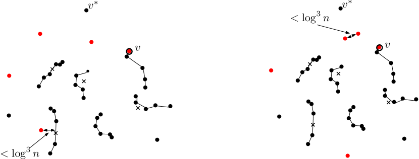
Figure 5: Illustration of the death rule in exploration process II. A snapshot of the revealed vertices when we are exploring the circled vertex $v$ is given. The black vertices and edges correspond to neutral and active vertices, while the crosses correspond to dead vertices. We are exploring $v$ and $mark(v)$ is denoted by the red vertices. On the left: a red vertex comes within distance $\log^{3}n$ of one the revealed vertices, hence death rule is satisfied. On the right: two of the revealed vertices are within distance $\log^{3}n$. Hence death rule is satisfied.

Threshold rule:

We stop if the number of steps exceed $n^{3/4}$ or $r$ exceeds $\log^{2}n$. Let $\delta$ denote the step when we stop stage $1$ of the exploration procedure.

Exploration process II, stage 2:

Similarly as in stage $1$, we start with $R^{\prime}_{0}={v_{2}}$ being active and $Q^{\prime}_{0}=mark(v_{2})\setminus v_{2}$ being dead. We proceed exactly as in stage $1$, except for the following change: if $v_{2}$ is a neighbour of $R_{\delta}\cup Q_{\delta}$, or while exploring $v$, if any of the vertices in $mark(v_{-})$ is a neighbour of $R_{\delta}\cup Q_{\delta}$, we say a collision has occurred and terminate the procedure.

We shall see later (see Lemmas 5.8 and 5.9) that with high probability, we perform the exploration for $n^{3/4}$ steps and the number of rounds is approximately $\log n$ in stage $1$. Also in stage $2$, collision occurs with high probability and the number of rounds is at most $\log n$ with high probability.

In what follows, we shall denote by $X^{\prime}$ in stage $2$ the set or variable corresponding to that denoted by $X$ in stage $1$ (for example, $R_{k}^{\prime},Q_{k}^{\prime}$ will denote the set of revealed subgraphs and dead vertices respectively up to stage $k$ in stage $2$ etc.)

Now we shall define a new tree $T_{C}$ which is defined on a subset of vertices of $t$. The tree $T_{C}$ will capture the growth process associated with the exploration process. We start with the tree $t$ and remove all its edges so we are left with only its vertices. The root vertex of $T_{C}$ is $v_{1}$. For every step of exploring $v$, we add an edge beween $v$ and every vertex of $mark(v_{-})$ (where $v_{-}$ is defined as in growth rule) in $T_{C}$ if death rule is not satisfied. Otherwise we add an edge between $v$ and $v_{-}$ in $T_{C}$. The vertices we connect by an edge to $v$ while exploring $v$ is called the offsprings of $v$ in $T_{C}$ similar in spirit to a Galton-Watson tree. It is clear that $T_{C}$ is a tree (since we terminate the procedure if $v_{-}\in R_{k}$). Let $Z_{r}$ denotes the number of vertices at distance $r$ from $v_{1}$ in $T_{C}$. Clearly, if we glue together vertices with the same mark which are at a distance at most $r$ in $T_{C}$, we obtain a subgraph of the ball of radius $r$ in the underlying graph of ${T}_{\lambda}(n)$. We similarly define another tree corresponding to stage $2$ of the process which we call $T_{C}^{\prime}$ which starts from the root vertex $v_{2}$.

Lemma 5.2.

The volume of $R_{\delta}\cup Q_{\delta}$ is at most $C_{0}n^{3/4}\log n$. Also the volume of $R_{\delta^{\prime}}\cup Q_{\delta^{\prime}}$ is at most $C_{0}n^{3/4}\log n$ where $C_{0}$ is as in part (i) of condition $(A)$.

Proof.

In every step, at most $C_{0}\log n$ vertices are revealed by condition $(A)$. ∎

Define $v_{1}$ and $v_{2}$ to be the seeds revealed in the first step. While exploring vertex $v$, we call the vertices in $mark(v_{-})\setminus v_{-}$ to be the seeds revealed at that step if the death rule is not satisfied. Note that because of the prescription of the death rule, seeds are necessarily isolated vertices (not a neighbour of any other revealed neutral or dead vertex up to that step.)

Definition 6.

A worm corresponding to a seed $s$ denotes a sequence of vertices $\{w_{0},w_{1},w_{2},\ldots,w_{d}\}$ such that $w_{0}$ is $s$ and $w_{i+1}$ is the vertex ${w_{i}}_{-}$ for $i\geq 0$.

Note that in the above definition, ${w_{i}}_{-}$ depends on the vertices revealed up to the time we explore $w_{i}$ in exploration process II.

Figure 6: An illustration of a worm at a certain step in the exploration process. The black vertices denote the vertices of the worm, the crosses are the dead vertices and the head of the worm is as shown. The circle is the $v_{*}$-ancestor of the head which is not dead. This worm has faced death $5$ times so far.

Note that in a worm, $w_{i+1}$ is a neighbour of $w_{i}$ if the $v_{*}$-parent of $w_{i}$ is not a dead vertex. If it is a dead vertex we move on to the next nearest ancestor of $w_{i}$ which is not dead. Note that the ancestors of $w_{i}$ which lie on the path joining $w_{i+1}$ and $w_{i}$ are necessarily dead. If there are $p$ dead vertices on the path between $w_{0}$ and the nearest $v_{*}$-ancestor of $w_{d}$ which is not dead, we say that the worm has faced death $p$ times so far (see Figure 6.) Call $w_{d}$ the head of the worm. The length of the worm is the distance in $U_{0,n}$ between $w_{d}$ and $w_{0}$.

We want the worms to remain disjoint so that conditioned up to the previous step, the number of children of a vertex in the tree $T_{C}$ or $T_{C}^{\prime}$ remain independent of the conditioning. Now for any worm, if $w_{i}\in N_{r}$ (resp. $w_{i}\in N_{r}^{\prime}$), then it is easy to see that $w_{i+1}\in N_{r+1}$ (resp. $w_{i+1}\in N_{r+1}^{\prime}$) because of the way the exploration process evolves. Hence if none of the worms revealed during the exploration process face a dead vertex, then the length of each worm is at most $\log^{2}n$ from threshold rule. Since every seed is at a distance at least $\log^{3}n$ from any other seed via the death rule, the worms will remain disjoint from each other if death does not occur.

Unfortunately, many worms will face a dead vertex with reasonable chance. But fortunately, none of them will face many dead vertices with high probability. We say that a disaster has occurred at step $k$ if after performing step $k$, there is a worm which has faced death at least $16$ times. The following proposition is immediate from the threshold rule for exploration process II and the discussion above.

Proposition 5.3.

If disaster does not occur, then the length of each worm is at most $\log^{2}n+16$ and hence no two worms intersect during the exploration process for large enough $n$.

We will now provide a series of Lemmas using which we will prove Theorem 5.1. The proofs of Lemmas 5.4 and 5.6 are postponed to Section 5.1 for clarity.

We start with a Lemma that shows that disaster does not happen with high probability and consequently the length of each worm is at most $\log^{2}n+16$ with high probability.

Lemma 5.4.

With $\mathbb{P}_{\lambda}$-probability at least $1-cn^{-3}$ disaster does not occur where $c>0$ is some constant.

Lemma 5.5.

Suppose disaster does not occur and $r\geq 0$. Then in the tree $T_{C}$, for $v\in Z_{r}$, $d^{T_{C}}(v,v_{1})<16r$. Also in $T_{C}^{\prime}$, for $v\in Z_{r}^{\prime}$, $d^{T_{C}^{\prime}}(v,v_{2})<16r$.

Proof.

We prove only for stage $1$ as for stage $2$ the proof is similar. The Lemma is trivially true for $r=0$. Suppose now the Lemma is true for $r^{\prime}=r$. Now for any vertex in $Z_{r}$ and its offspring, the vertices corresponding to their marks in the underlying graph of ${T}_{\lambda}(n)$ must lie at a distance at most $16$ because otherwise disaster would occur. Hence the distance of every vertex in $Z_{r+1}$ from $v_{1}$ is at most $16r+16=16(r+1)$. We use induction to complete the proof. ∎

Let $\mathcal{E}$ (resp. $\mathcal{E}^{\prime}$) be the event that disaster has not occurred up to step $\delta$ (resp. $\delta^{\prime}$). Let $\mathcal{F}_{k}$ denote the sigma field generated by $R_{0},\ldots,R_{k},Q_{0},\ldots,Q_{k}$. Let $\mathcal{F}_{k}^{\prime}$ denote the sigma field $\sigma(R_{0}^{\prime},\ldots,R_{k}^{\prime},Q_{0}^{\prime},\ldots,Q_{k}^{\prime})\vee\mathcal{F}_{\delta}$. Let $v_{k+1}$ (resp. $v_{k+1}^{\prime}$) be the vertex we explore in the $k+1$th stage in the exploration process stage $1$ (resp. stage $2$).

Lemma 5.6.

Conditioned on $\mathcal{F}_{k}$ (resp. $\mathcal{F}_{k}^{\prime}$) such that $k<\delta$ (resp. $\delta^{\prime}$) and disaster has not occurred up to step $k$, the $\mathbb{P}_{\lambda}$-probability that $v_{k+1}$ in $T_{C}$ (resp. $T_{C}^{\prime}$) has

• no offsprings is $0$.

• at least $3$ offsprings is at least $k_{0}$ for some constant $k_{0}>0$.

We will now construct a supercritical Galton-Watson tree which is stochastically dominated by both $T_{C}$ and $T_{C}^{\prime}$. Consider a Galton-Watson tree $GW$ with offspring distribution $\xi$ where

• $\mathbb{P}(\xi=1)=(1-k_{0}/2)$

• $\mathbb{P}(\xi=2)=k_{0}/2$

and $k_{0}$ is the constant obtained in part (ii) of Lemma 5.6. Let $Z^{GW}_{r}$ be the number of offsprings in the $r$-th generation of $GW$. Lemma 5.6 and the definition of $GW$ clearly shows that $Z_{r}$ stochastically dominates $Z^{GW}_{r}$ for all $r\geq 1$ if disaster does not occur up to step $\tau_{r}$. Let $r_{\delta}=\max\{r:\tau_{r}<\delta\}$ and similarly define $r_{\delta^{\prime}}=\max\{r:\tau_{r}<\delta^{\prime}\}$. Thus, we have

Lemma 5.7.

For any integer $j\leq r_{\delta}$ (resp. $j\leq r_{\delta^{\prime}}$), $Z_{j}$ stochastically dominates $Z^{GW}_{j}$ on the event $\mathcal{E}$ (resp. $\mathcal{E}^{\prime}$).

It is clear that the mean offspring distribution of $GW$ is strictly greater than $1$ and hence $GW$ is a supercritical Galton-Watson tree. Also $GW$ is infinite with probability $1$.

Now we are ready to show that the depth of $T_{C}$ (resp. $T_{C}^{\prime}$) when we run the exploration upto time $\delta$ (resp. $\delta^{\prime}$) is of logarithmic order with high probability.

Lemma 5.8.

There exists a $C>0$ such that

• $\mathbb{P}_{\lambda}((r_{\delta}>C\log n)\cap\mathcal{E})=O(n^{-3})$

• $\mathbb{P}_{\lambda}((r_{\delta^{\prime}}>C\log n)\cap\mathcal{E}^{\prime})=O(n^{-3})$

Proof.

We shall prove only (i) as proof of (ii) is similar. Because of Lemmas 5.7 and 5.2 we have for a large enough choice of $C>0$,

$$\mathbb{P}_{\lambda}((r_{\delta}>C\log n)\cap\mathcal{E}) <\mathbb{P}_{\lambda}\left(\sum_{i=1}^{\lfloor C\log n\rfloor}Z^{GW}_{i}\leq C_{0}n^{3/4}\log n\right)$$

$$<\mathbb{P}_{\lambda}\left(Z^{GW}_{\lfloor C\log n\rfloor}\leq C_{0}n^{3/4}\log n\right)$$

$$<n^{-3}$$ (5.1)

where (5.1) follows by applying Lemma 2.5, choosing $C>0$ large enough and observing the fact that $\mathbb{P}_{\lambda}(Z_{r}=0)=0$ for any $r$ from definition of $GW$. ∎

Recall that in stage $2$, we stop the process if we have revealed a vertex which is a neighbour of $R_{\delta}\cup Q_{\delta}$, and we say a collision has occurred. Let us denote the event that collision does not occur up to step $k$ by $\mathcal{C}_{k}$. Since $\delta\leq\lfloor n^{3/4}\rfloor$ implies either disaster has occurred in stage $1$ or $r_{\delta}>\log^{2}n$ and $\delta^{\prime}\leq\lfloor n^{3/4}\rfloor$ implies either disaster has occurred in stage $2$ or $r_{\delta}^{\prime}>\log^{2}n$ or a collision has occurred we have the immediate corollary

Corollary 5.9.

On the event $\mathcal{E}$, the $\mathbb{P}_{\lambda}$-probability that $\delta\leq\lfloor n^{3/4}\rfloor$ is $O(n^{-3})$. On the event $\mathcal{E}^{\prime}\cap\mathcal{C}_{\delta^{\prime}}$, the $\mathbb{P}_{\lambda}$-probability that $\delta^{\prime}\leq\lfloor n^{3/4}\rfloor$ is $O(n^{-3})$.

Now we are ready to prove our estimate on the typical distances. We show next, that a collision will occur with high probability.

Lemma 5.10.

Probability that a collision occurs before step $\delta^{\prime}$ is at least $1-cn^{-3}$ for some constant $c>0$.

Proof.

Let $\mathcal{H}$ be the event that disaster does not occur up to step $\delta$, $\delta=\lfloor n^{3/4}\rfloor+1$. Let $A(R_{\delta})$ be the set of $v_{*}$- parents of the heads of the worms in $R_{\delta}$. Since at each step at least one vertex is revealed, $\delta=\lfloor n^{3/4}\rfloor+1$ implies the number of vertices revealed is at least $n^{3/4}$. If disaster does not occur, then from Lemmas 5.4 and 5.3, the worms are disjoint and each worm has length at most $\log^{2}n+16$. Hence the number of vertices in $A(R_{\delta})$ is at least $n^{3/4}/(\log^{2}n+16)$. Also, the number of vertices in $A(R_{\delta})$ is at most $C_{0}n^{3/4}\log n$ from Lemma 5.2. For any $k<\delta^{\prime}$, conditioned on the event $\mathcal{C}_{k}$ that no collision has occured up to step $k$, the probability that collision occurs in step $k+1$ when we are exploring a vertex $v$ is at least (using Bonferroni’s inequality),

$$\sum_{w\in A(R_{\delta})}\mathbb{P}_{\lambda}(m(v)=m(w)|\mathcal{C}_{k},\mathcal{H})-\sum_{w,z\in A(R_{\delta})}\mathbb{P}_{\lambda}(m(v)=m(w)=m(z)|\mathcal{C}_{k},\mathcal{H})$$

$$>\frac{c}{n^{1/4}\log^{2}n}-\frac{c\log^{2}n}{\sqrt{n}}$$ (5.2)

$$>\frac{c}{n^{1/4}\log^{2}n}$$ (5.3)

for some constant $c>0$. The first term of (5.2) follows from the lower bound of (2.3). The second term of (5.2) follows from (2.4) and noting that the number of terms in the sum is $O(n^{3/2}\log^{2}n)$. Since the bound on the probability displayed in (5.3) is independent of the conditioning,

$$\mathbb{P}_{\lambda}(\mathcal{C}_{\delta^{\prime}}\cap\delta^{\prime}=\lfloor n^{3/4}\rfloor+1|\mathcal{H})+\mathbb{P}_{\lambda}(\mathcal{C}_{\delta^{\prime}}\cap\delta^{\prime}\leq\lfloor n^{3/4}\rfloor|\mathcal{H})$$

$$< \left(1-\frac{c}{n^{1/4}\log^{2}n}\right)^{n^{3/4}}+\mathbb{P}_{\lambda}(\mathcal{C}_{\delta^{\prime}}\cap\mathcal{E}^{\prime}\cap\delta^{\prime}\leq\lfloor n^{3/4}\rfloor|\mathcal{H})+\mathbb{P}_{\lambda}((\mathcal{E}^{\prime})^{c}|\mathcal{H})$$

$$< \exp(-c\sqrt{n}/\log^{2}n)+O(n^{-3})$$ (5.4)

$$= O(n^{-3})$$

where the bound on the second term in eq. 5.4 follows from Corollaries 5.9 and 5.4. The Lemma now follows because the probability of the complement of $\mathcal{H}$ is $O(n^{-3})$ again from Corollaries 5.9 and 5.4. ∎

Proof of Theorem 5.1.

Suppose we have performed exploration process I stage 1 and 2. Let $\mathcal{G}$ be the event that $r_{\delta}\leq C\log n,r_{\delta^{\prime}}\leq C\log n$, disaster does not occur before step $\delta$ or $\delta^{\prime}$ and a collision occurs. On the event $\mathcal{G}$ the distance between $V_{1}$ and $V_{2}$ in the underlying graph of ${T}_{\lambda}(n)$ is at most $32C\log n+1$ by Lemma 5.5. But by Lemmas 5.4, 5.10 and 5.8, the complement of the event $\mathcal{G}$ has probability $O(n^{-3})$. ∎

5.1 Remaining proofs

The proofs of both the Lemmas in this subsection are for stage $1$ of the exploration process as the proof for stage $2$ is the same.

Proof of Lemma 5.4.

Let $s$ be a seed revealed in the $k$th step of exploration process II . Suppose $P$ denotes the set of vertices at a distance at most $\log^{2}n+16$ from $s$ along the unique path joining $s$ and $v_{*}$. Note that none of the vertices in $P$ are revealed yet because of the death rule. If the worm corresponding to $s$ faces more than $16$ dead vertices, then more than $16$ dead vertices must be revealed in $P$ during the exploration from step $k$ to $\delta$. Conditioned up to the previous step, the probability that one of the revealed vertices lie in $P$ in a step is $O(n^{-1}(\log^{2}n+16))$ from (2.3) and union bound. Since this bound is independent of the conditioning, the probability that this event happens at least $16$ times during the process is $O(n^{-16}\log^{32}n\cdot n^{12})=O(n^{-4}\log^{32}n)$ where the factor $n^{12}$ has the justification that $\dbinom{\lfloor n^{3/4}\rfloor}{16}=O(n^{12})$ is the number of combination of steps by which this event can happen $16$ times. Observe that more than one vertex may be revealed in $P$ in a step, but the probability of that event is even smaller. Thus taking union over all seeds, we see that the probability of disaster occurring is $O(n^{-13/4}\log^{33}n)=O(n^{-3})$ using Lemma 5.2 and union bound. ∎

Proof of Lemma 5.6.

It is clear that on the event of no disaster, every explored vertex has at least the offspring corresponding to its closest non-dead $v_{*}$-ancestor in the tree $T_{C}$. This is because on the event of no disaster, no two worms intersect. For stage $2$, the closest non-dead $v_{*}$-ancestor cannot belong to $R_{\delta}\cup Q_{\delta}$ because otherwise, the process would have stopped. Hence (i) is trivial.

Now for (ii), first recall that condition $(A)$ ensures that the number of indices $i$ such that $\lambda_{i}\geq 3$ is at least $(1-d_{2})n$. Now since the number of vertices revealed upto any step $k<\delta$ is $O(n^{3/4}\log n)$, the number of vertices left with mark $i$ such that $\lambda_{i}\geq 3$ is at least $(1-d_{2})n-O(n^{3/4}\log n)>(1-d_{2})n/2$ for large enough $n$. Note that the number of offsprings of $v$ in $T_{C}$ is at least $3$ if the number of vertices with the same mark as $v_{-}$ is at least $3$ and death does not occur. Hence if we can show that the probability of death rule being satisfied in a step is $o(1)$, we are done.

To satisfy the death rule in step $k+1$, a vertex in $mark(v_{-})\setminus v_{-}$ must be within distance $\log^{3}n$ in the tree $U_{0,n}$ to another vertex in $mark(v_{-})\setminus v_{-}$ or $R_{k}\cup Q_{k}\cup v^{*}$. Now using of part (ii) of condition $(B)$ and Lemma 5.2, the number of vertices within $\log^{3}n$ of $R_{\delta}\cup Q_{\delta}\cup v^{*}$ is $O(n^{3/4}\log^{9}n)$. Hence the probability that the death rule is satisfied is $O(n^{-1/4}\log^{9}n)=o(1)$ by union bound. This completes the proof. ∎

Appendix A Proof of Lemma 2.3

We shall prove Lemma 2.3 in this section. We do the computation following the method of random allocation similar in lines of [22]. For this, we need to introduce i.i.d. random variables $\{\xi_{1},\xi_{2},\ldots\}$ such that for some parameter $\beta\in(0,1)$

$$P(\xi_{1}=2i+1)\begin{cases}=\frac{\beta^{2i+1}}{B(\beta)(2i+1)}&\mbox{if }i\in\mathbb{N}\cup\{0\}\\ =0&\mbox{otherwise}\end{cases}$$ (A.1)

where $B(\beta)=1/2\log((1+\beta)/(1-\beta))$. Recall that $\mathcal{P}$ is the set of all $N$-tuples of odd positive integers which sum up to $n+1$. Observe that for any $z=(z_{1},\ldots,z_{N})\in\mathcal{P}$,

$$P(\lambda=z)=P(\xi_{1}=z_{1},\ldots,\xi_{N}=z_{N}|\xi_{1}+\xi_{2}+\ldots\xi_{N}=n+1)$$

throughout this Section, we shall assume the following:

• $\{n,N\}\to\{\infty,\infty\}$ and $n/N\to\alpha$ for some constant $\alpha>1$.

• For every $n$, the parameter $\beta=\beta(n)$ is chosen such that $E(\xi_{1})=m=(n+1)/N$

It is easy to check using (A.1) that there is a unique choice of such $\beta$ and $\beta$ converges to some finite number $\beta_{\alpha}$ such that $0<\beta_{\alpha}<1$ as $(n+1)/N$ converges to $\alpha$. Let $\zeta_{N,j}=\xi_{1}^{j}+\ldots\xi_{N}^{j}$ where $j\geq 1$ is an integer. It is also easy to see that for any integer $j\geq 1$, $\mathbb{E}\xi_{1}^{j}=m_{j}(n)$ for some function $m_{j}$ which also converge to some number $m_{j\alpha}$ as $n\to\infty$. Let $\sigma_{j}^{2}=Var(\xi_{1}^{j})$. To simplify notation, we shall denote $\zeta_{N,1}$ by $\zeta_{N}$ and $\sigma_{1}$ by $\sigma$.

We will first prove a central limit theorem for $\zeta_{N}$.

Lemma A.1.

We have,

$$\frac{\zeta_{N}-Nm}{\sigma\sqrt{N}}\to N(0,1)$$ (A.2)

in distribution as $n\to\infty$.

Proof.

Easily follows by checking the Lyapunov condition for triangular arrays of random variables (see [18]). ∎

We now prove a local version of the CLT asserted by Lemma A.1.

Lemma A.2.

We have

$$P(\zeta_{N}=n+1)\sim\frac{2}{\sqrt{2\pi N}\sigma}$$

Proof.

Let $\overline{\xi_{i}}=(\xi_{i}-1)/2$. Apply Theorem $1.2$ of [16] for the modified arrays $\{\overline{\xi_{1}},\ldots\overline{\xi_{N}}\}_{n\geq 1}$ and use Lemma A.1. The details are left for the readers to check. ∎

Lemma A.3.

Fix $j\geq 1$. There exists constants $C_{1}>1$ and $C_{2}>1$ (both depending only on $\alpha$ and $j$) such that

$$P\left(C_{1}n<\sum_{i=1}^{N}\lambda_{i}^{j}<C_{2}n\right)>1-\frac{c}{n^{7/2}}$$ (A.3)

for some $c>0$ which again depends only on $\alpha$ and $j$ for large enough $n$.

Proof.

It is easy to see that $m_{j}\to m_{j\alpha}$ as $n\to\infty$. Notice that

$$P\left(\sum_{i=1}^{N}\lambda_{i}^{j}>C_{2}n,\sum_{i=1}^{N}\lambda_{i}^{j}<C_{1}n\right) =P\left(\zeta_{N,j}>C_{2}n,\zeta_{N,j}<C_{1}n|\zeta_{N}=n\right)$$

$$<\frac{P\left(\zeta_{N,j}>C_{2}n,\zeta_{N,j}<C_{1}n\right)}{P(\zeta_{N}=n)}$$ (A.4)

Choose $C_{2}>m_{j\alpha}$ and $C_{1}<m_{j\alpha}$. Then for some $c>0$, for large enough $n$,

$$P\left(\zeta_{N,j}>C_{2}n,\zeta_{N,j}<C_{1}n\right)<P\left(|\zeta_{N,j}-m_{j}N|>cn\right)<\mathbb{E}\left(\zeta_{N,j}-m_{j}N\right)^{8}(cn)^{-8}$$ (A.5)

It is easy to see that $\mathbb{E}\left(\zeta_{N,j}-m_{j}N\right)^{8}=O(n^{4})$ since the terms involving $\mathbb{E}(\xi_{i}^{j}-m_{j})$ vanishes and all the finite moments of $\xi_{1}$ are bounded. Now plugging in this estimate into eq. A.5, we get

$$P\left(\zeta_{N,j}>C_{2}n,\zeta_{N,j}<C_{1}n\right)=O(n^{-4})$$ (A.6)

Now plugging in the estimate of eq. A.6 into eq. A.4 and observing that $P(\zeta_{N}=n)\asymp N^{-1/2}$ via Lemma A.2, the result follows. ∎

Lemma A.4.

There exists a constant $C_{0}>0$ such that

$$P(\lambda_{\max}>C_{0}\log n)=O(n^{-3})$$

Proof.

Let $\xi_{\max}$ be the maximum among $\xi_{1},\ldots,\xi_{N}$. Note that

$$\mathbb{P}(\xi_{\max}>C_{0}\log n)<N\mathbb{P}(\xi_{1}>C_{0}\log n)=O(N\beta^{C_{0}\log n})=O(n^{-7/2})$$ (A.7)

if $C_{0}>0$ is chosen large enough. Now the Lemma follows from the estimate of Lemma A.2. The details are left to the reader. ∎

Lemma A.5.

There exists constants $0<d_{1}<1$ and $0<d_{2}<1$ which depends only on $\alpha$ such that $\mathbb{P}(d_{1}n<|i:\lambda_{i}=1|<d_{2}n)<e^{-cn}$ for some constant $c>0$ for large enough $n$.

Proof.

The probability that $|i:\lambda_{i}=1|<d_{2}n$ for large enough $n$ for some $0<d_{2}<1$ follows directly from the fact that $|i:\lambda_{i}=1|\leq N$. For the upper bound,

$$\mathbb{P}(|i:\lambda_{i}=1|>d_{1}n)=\mathbb{P}\left(\sum_{i=1}^{N}1_{\lambda_{i}=1}>d_{1}n\right)<\frac{\mathbb{P}\left(\sum_{i=1}^{N}1_{\xi_{i}=1}>d_{1}n\right)}{\mathbb{P}(\zeta_{N}=n)}$$ (A.8)

Now $\mathbb{P}(\xi_{i}=1)\to\beta_{\alpha}/B(\beta_{\alpha})$ as $n\to\infty$. The Lemma now follows by choosing $d_{1}$ small enough, applying Lemma A.2 to the denominator in eq. A.8 and a suitable large deviation bound on Bernoulli variables. Details are standard and is left to the reader. ∎

Proof of Lemma 2.3.

Follows from Lemmas A.3, A.5 and A.4. ∎

Appendix B Proofs of the lemmas in Section 2.3

In this section, we shall prove Lemmas 2.5 and 2.7.

Let $p_{i}$ denote $\mathbb{P}(\xi=i)$ for $i\in\mathbb{N}$ and denote the generating function by $\varphi(s)=\sum_{i}p_{i}s^{i}$. Let $\mu=\mathbb{E}\xi$. Let $Z_{n}$ denote the number of offsprings in the $n$-th generation of the Galton-Watson process

B.1 Critical Galton-Watson trees

We assume $\xi$ has geometric distribution with parameter $1/2$. Here $\mu=1$ and we want to show that $Z_{r}$ cannot be much more than $r$. The following large deviation result is a special case of the main theorem of [27].

Proposition B.1.

For all $r\geq 1$ and $k\geq 1$,

$$\mathbb{P}(Z_{r}\geq k)<\frac{3}{2}\left(1+\frac{1}{\varphi^{\prime\prime}(3/2)r/2+2}\right)^{-k}$$

B.2 Supercritical Galton-Watson trees

Here $\mu>1$. Recall the assumptions

• $0<p_{0}+p_{1}<1$

• There exists a small enough $\lambda>0$ such that $\mathbb{E}(e^{\lambda\xi})<\infty$.

It is well known (see [21]) that $Z_{n}/\mu^{n}$ is a martingale which converges almost surely to some non-denegerate random variable $W$. Let $\rho:=P(\lim_{n}Z_{n}=0)$ be the extinction probability which is strictly less than $1$ in the supercritical regime.

The following results may be realized as special cases of the results in [7], [19] and further necessary references can be found in these papers.

$W$ if restricted to $(0,\infty)$ has a strictly positive continuous density which is denoted by $w$. In other words, we have the following limit theorem:

$$\lim_{n}\mathbb{P}(Z_{n}\geq x\mu^{n})=\int_{x}^{\infty}w(t)dt,\quad\quad x>0$$

Also define $\gamma:=\varphi^{\prime}(\rho)$ where $0<\gamma<1$ in our case. Define $\beta$ by the relation $\gamma=\mu^{-\beta}$. It is clear that in our case $\beta\in(0,\infty)$. $\beta$ is used to determine the behaviour of $w$ as $x\downarrow 0$. The following is proved in [7].

Proposition B.2.

Let $\eta:=\mu^{\beta/(3+\beta)}>1$. Then for all $\varepsilon\in(0,\eta)$, there exists a positive constant $C_{\varepsilon}>0$ such that for all $k\geq 1$,

$$\lvert\mathbb{P}(Z_{r}=k)\mu^{r}-w(k/\mu^{r})\rvert\leq C_{\varepsilon}\frac{\eta^{-r}}{k\mu^{-r}}+(\eta-\varepsilon)^{-r}$$ (B.1)

for all $r\geq 1$.

It can be shown (see [12]) that there exists positive constants $A_{1}>0,A_{2}>0$ such that $A_{1}x^{\beta-1}<w(x)<A_{2}x^{\beta-1}$ as $x\downarrow 0$. Using this and eq. B.1, we get

$$\mathbb{P}(Z_{r}=k)\leq C\frac{k^{\beta-1}}{\mu^{r\beta}}+\frac{\eta^{-r}}{k}+((\eta-\varepsilon)\mu)^{-r}$$ (B.2)

Proof of Lemma 2.5.

The proof is straightforward by summing $k$ from $1$ to $\gamma^{r}$ the expression given by the right hand side of (B.2). ∎

B.3 Random plane trees

Proof of Lemma 2.7.

Note that it is enough to prove the bound for $r\leq n$ because otherwise the probability is $0$. It is well known that if we pick an oriented edge uniformly from $U_{0,n}$ and re-root the tree there then the distribution of this new re-rooted tree is the same as that of $U_{0,n}$ (see [17]). Let $V$ denote the root vertex of the new re-rooted tree and let $\mathcal{Z}_{j}(V)$ denote the number of vertices at distance exactly $j$ from $V$. It is well known that the probability of a critical geometric Galton-Watson tree to have $n$ edges is $\asymp n^{-3/2}$. Using this fact and Proposition B.1 we get for any $k\geq 1$ and $1\leq j\leq r$

$$\mathbb{P}(\mathcal{Z}_{j}(V)>k)<n^{3/2}c\exp(-c^{\prime}k/j)<n^{3/2}c\exp(-c^{\prime}k/r)$$ (B.3)

and some suitable positive constants $c,c^{\prime}$. Note that if $M_{r}>r^{2}\log^{2}n$ then $\mathcal{Z}_{j}(v)>r\log^{2}n$ for some $1\leq j\leq r$ and some vertex $v\in U_{0,n}$. Using this and union bound to the estimate obtained in (B.3), we get

$$\mathbb{P}(M_{r}>r^{2}\log^{2}n)<cn^{5/2}r\exp(-c^{\prime}\log^{2}n)=O(\exp(-c^{\prime}\log^{2}n))$$

for some positive constants $c$ and $c^{\prime}$. This completes the proof. ∎

Gourab Ray, UBC, <gourab1987@gmail.com>

References

- [1] L. Addario-Berry, L. Devroye, and S. Janson. Sub-Gaussian tail bounds for the width and height of conditioned Galton-Watson trees. Ann. Probab., 41(2):1072–1087, 2013.
- [2] D. Aldous. The continuum random tree. I. Ann. Probab., 19(1):1–28, 1991.
- [3] O. Angel. Growth and percolation on the uniform infinite planar triangulation. Geom. Funct. Anal., 13(5):935–974, 2003.
- [4] O. Angel, G. Chapuy, N. Curien, and G. Ray. The local limit of unicellular maps in high genus. Elec. Comm. Prob, 18:1–8, 2013.
- [5] O. Angel and G. Ray. Classification of half planar maps. Ann. Probab., 2013. To appear. ArXiv:1303.6582.
- [6] O. Angel and O. Schramm. Uniform infinite planar triangulations. Comm. Math. Phys., 241(2-3):191–213, 2003.
- [7] K. Athreya and P. Ney. The local limit theorem and some related aspects of supercritical branching processes. Trans. Amer. Math. Soc., 152(2):233–251, 1970.
- [8] I. Benjamini. Euclidean vs graph metric. www.wisdom.weizmann.ac.il/ itai/erd100.pdf.
- [9] I. Benjamini and O. Schramm. Recurrence of distributional limits of finite planar graphs. Electron. J. Probab., 6:no. 23, 1–13, 2001.
- [10] O. Bernardi. An analogue of the Harer-Zagier formula for unicellular maps on general surfaces. Adv. in Appl. Math., 48(1):164–180, 2012.
- [11] J. Bettinelli. Scaling limits for random quadrangulations of positive genus. Electron. J. Probab., 15:no. 52, 1594–1644, 2010.
- [12] J. D. Biggins and N. H. Bingham. Large deviations in the supercritical branching process. Adv. in Appl. Probab., 25(4):757–772, 1993.
- [13] G. Chapuy. A new combinatorial identity for unicellular maps, via a direct bijective approach. Adv. in Appl. Math., 47(4):874–893, 2011.
- [14] G. Chapuy, V. Féray, and É. Fusy. A simple model of trees for unicellular maps. Journal of Combinatorial Theory, Series A, 120(8):2064–2092, 2013.
- [15] G. Chapuy, M. Marcus, and G. Schaeffer. A bijection for rooted maps on orientable surfaces. SIAM J. Discrete Math., 23(3):1587–1611, 2009.
- [16] B. Davis and D. McDonald. An elementary proof of the local central limit theorem. J. Theoret. Probab., 8(3):693–701, 1995.
- [17] L. Devroye and S. Janson. Distances between pairs of vertices and vertical profile in conditioned Galton-Watson trees. Random Structures Algorithms, 38(4):381–395, 2011.
- [18] R. Durrett. Probability: theory and examples. Cambridge Series in Statistical and Probabilistic Mathematics. Cambridge University Press, Cambridge, fourth edition, 2010.
- [19] K. Fleischmann and V. Wachtel. Lower deviation probabilities for supercritical Galton-Watson processes. Ann. Inst. H. Poincaré Probab. Statist., 43(2):233–255, 2007.
- [20] M. Gromov. Metric structures for Riemannian and non-Riemannian spaces. Modern Birkhäuser Classics. Birkhäuser Boston Inc., Boston, MA, english edition, 2007. Based on the 1981 French original, With appendices by M. Katz, P. Pansu and S. Semmes, Translated from the French by Sean Michael Bates.
- [21] T. E. Harris. The theory of branching processes. Dover Phoenix Editions. Dover Publications Inc., Mineola, NY, 2002. Corrected reprint of the 1963 original [Springer, Berlin; MR0163361 (29 #664)].
- [22] N. I. Kazimirov. The occurrence of a gigantic component in a random permutation with a known number of cycles. Diskret. Mat., 15(3):145–159, 2003.
- [23] H. Kesten. Subdiffusive behavior of random walk on a random cluster. Ann. Inst. H. Poincaré Probab. Statist., 22(4):425–487, 1986.
- [24] M. Krikun. Local structure of random quadrangulations. arXiv:math/0512304, 2005.
- [25] S. K. Lando and A. K. Zvonkin. Graphs on surfaces and their applications, volume 141 of Encyclopaedia of Mathematical Sciences. Springer-Verlag, Berlin, 2004. With an appendix by Don B. Zagier, Low-Dimensional Topology, II.
- [26] J. F. Le Gall. Random trees and applications. Probab. Surv, 2:245–311, 2005.
- [27] S. V. Nagaev and N. V. Vahrusev. Estimation of probabilities of large deviations for a critical Galton-Watson process. Theory Probab. Appl., 20(1):179–180, 1975.