Fast inverse transform sampling in one and two dimensions
Abstract
We develop a computationally efficient and robust algorithm for generating pseudo-random samples from a broad class of smooth probability distributions in one and two dimensions. The algorithm is based on inverse transform sampling with a polynomial approximation scheme using Chebyshev polynomials, Chebyshev grids, and low rank function approximation. Numerical experiments demonstrate that our algorithm outperforms existing approaches.
1 Introduction
Generating pseudo-random samples from a prescribed probability distribution is an important task in applied probability, statistics, computing, physics, and elsewhere. A classical approach is inverse transform sampling, in which pseudo-random samples are generated from a uniform distribution on and then transformed by , where is the cumulative distribution function (CDF) of a prescribed probability distribution.
Conventional wisdom is that the practical application of inverse transform sampling is limited. To quote (GentleSampling, , pp. 103):
[Inverse transform sampling] requires a complete approximation to [the CDF] regardless of the desired sample size, it does not generalize to multiple dimensions and it is less efficient than other approaches.
Similar comments are present in other computational statistics texts, for example, (StatisticalAtmosphere, , pp. 124), (GivensComputationalStats, , pp. 155), and (TanizakiComputational, , pp. 122). Instead, other methods are advocated for low dimensions, such as slice sampling Neal_03_01 or rejection sampling TanizakiComputational ; StatisticalAtmosphere ; GentleSampling ; GivensComputationalStats . In higher dimensions, algorithms concentrate on avoiding the curse of dimensionality, such as Metropolis–Hastings sampling MetropolisSampling . Moreover, there are many other methods that are designed to exploit certain special properties: e.g., ziggurat algorithm Ziggurat (requires monotonicity) and adaptive rejection sampling Gilks_92_01 ; Gilks_92_02 (requires log-convexity).
In contradiction to conventional wisdom, we show that inverse transform sampling is computationally efficient and robust when combined with an adaptive Chebyshev polynomial approximation scheme. Approximation by Chebyshev polynomials converges superalgebraically fast for smooth functions, and hence the CDF can be numerically computed to very high accuracy, i.e., close to machine precision. Rather than forming the inverse CDF — which is often nearly singular — we invert the CDF pointwise using a simple bijection method. This approach is robust — it is guaranteed to converge to a high accuracy — and fast, due to the simple representation of the CDF.
Furthermore, we extend our approach to probability distributions of two variables by exploiting recent developments in low rank function approximation to achieve a highly efficient inverse transform sampling scheme in 2D. Numerical experiments confirm that this approach outperforms existing sampling routines for many black box distributions, see Section 4.
Remark 1
We use black box distribution to mean a continuous probability distribution that can only be evaluated pointwise111Strictly, we require the distribution to be continuous with bounded variation Trefethen_13_01 , and in practice this is almost always satisfied by continuous functions. We do not require the distribution to be prescaled to integrate to one, nor that the distribution decays smoothly to zero.. The only other piece of information we assume is an interval , or a rectangular domain , containing the numerical support of the distribution.
A Matlab implementation is publicly available from InverseTransformCode . As an example, the following syntax generates samples from a 2D distribution:
ΨΨ[X,Y] = sample(@(x,y) exp(-x.^2-2.*y.^2).*(x-y).^2,[-3,3],[-3,3],2000); Ψ
The algorithm scales the input function to integrate to one, and generates pseudo-random samples from the resulting probability distribution.
2 Inverse transform sampling with polynomial approximation
Let be a prescribed non-negative function supported on the interval . Otherwise, if the support of is the whole real line and is rapidly decaying, an interval can be selected outside of which is negligible. The algorithm will draw samples that match the probability distribution
up to a desired tolerance (typically close to machine precision such as ).
First, we replace by a polynomial approximant on , which we numerically compute such that . That is, we construct a polynomial approximant of in the form
| (1) |
where is the degree Chebyshev polynomial. While the polynomial approximants (1) could be represented in other polynomial bases — such as the monomial basis — the Chebyshev basis is a particularly good choice for numerical computation as the expansion coefficients can be stably calculated in operations Mason_03_01 ; Trefethen_13_01 . This is accomplished by applying the fast cosine transform to function evaluations of taken from a Chebyshev grid in of size , i.e., at the set of points
We can adaptively select by sampling at Chebyshev grids of size , , , and so on, until the tail of the coefficients has decayed to below machine precision relative to the absolute maximum of . In addition to the fast transform, Chebyshev expansions are numerically stable Trefethen_13_01 , in contrast to the well-known numerical instability associated to interpolation at equispaced points Platte_11_01 .
Instead of symbolically manipulating , which is not possible if is a black box distribution, we numerically manipulate to apply the inverse transform sampling approach. This rests on fast and well-established algorithms for evaluating and integrating polynomial interpolants of the form (1). (A convenient implementation of many of these algorithms is in the Chebfun software system Chebfun .) Figure 1 summarizes the approach we are about to describe based on the inverse transform sampling and Chebyshev approximation.
| Algorithm: Inverse transform sampling with Chebyshev approximation |
| Input: A non-negative function , a finite interval , and an integer . |
| Output: Random samples drawn from . |
| Construct an approximant of on . |
| Compute using (2). |
| Scale to a CDF, , if necessary. |
| Generate random samples from the uniform distribution on . |
| for |
| Solve for . |
| end |
With the polynomial approximation in hand, we construct the corresponding cumulative function, denoted by , by calculating the indefinite integral
where the last equality comes from a change of variables with . Fortunately, we have the following relation satisfied by Chebyshev polynomials (Mason_03_01, , pp. 32–33):
| (2) |
where . Therefore, using (2), we can compute coefficients in operations (see, for example, (Mason_03_01, , pp. 32–33)) such that
| (3) |
At this stage we rescale so that it is a CDF: .
Once we have the approximant , given in (3), we generate pseudo-random samples from the uniform distribution on using a standard inbuilt pseudo-random number generator, and then solve the following rootfinding problems for :
| (4) |
The rootfinding problems in (4) can be solved by various standard methods such as the eigenvalues of a certain matrix Trefethen_13_01 , Newton’s method, the bisection method, or Brent’s method (Brent_73_01, , Chapter 4).
To achieve robustness — guaranteed convergence, computation cost, and accuracy — we use the bisection method. The bisection method approximates the (unique) solution to by a sequence of intervals that contain , satisfying . The initial interval is the whole domain . Each stage finds the midpoint of the interval , choosing the new interval based on whether is greater or less than . Convergence occurs when , where . For example, it takes precisely 47 iterations to converge when and a further five iterations to converge to machine precision. Since the CDF is represented as a Chebyshev series (3) it can be efficiently evaluated using Clenshaw’s method, which is an extension of Horner’s scheme to Chebyshev series Clenshaw_55_01 .
The inverse transform sampling with Chebyshev approximation is very efficient, as demonstrated in the numerical experiments of Section 4 using the Matlab implementation InverseTransformCode .
3 Inverse transform sampling in two variables
We now extend the inverse transform sampling approach with Chebyshev approximation to probability distributions of two variables. Figure 2 summarizes our algorithm, which generates pseudo-random samples drawn from the probability distribution . The essential idea is to replace by a low rank approximant that can be manipulated in a computationally efficient manner. Again, for convenience, if is a non-negative function that does not integrate to one then we automatically scale the function to a probability distribution.
| Algorithm: Inverse transform sampling for |
|---|
| Input: A non-negative function , a finite domain , and an integer . |
| Output: Random samples from . |
| Construct a low rank approximant of on . |
| Compute . |
| Generate random samples from . |
| for |
| Generate a random sample from . |
| end |
We use a low rank approximation of . A rank- function is a function of two variables that can be written as the product of two univariate functions, i.e., . Moreover, a rank- function is a sum of rank-1 functions. We efficiently approximate a probability distribution by a rank- function by using Gaussian elimination Townsend_13_01 :
| (5) |
where is adaptively chosen and and are polynomials of one variable represented in Chebyshev expansions of the form (1). For simplicity we assume that and are polynomials of degree and , respectively, and then a function is considered to be of low rank if .
While most functions are mathematically of infinite rank — such as — they can typically be approximated by low rank functions to high accuracy, especially if the function is smooth Townsend_13_02 . It is well-known that the singular value decomposition can be used to compute optimal low rank approximations of matrices, and it can easily be extended for the approximation of functions. However, the Gaussian elimination approach from Townsend_13_01 is significantly faster and constructs near-optimal low rank function approximations Bebendorf_08_01 ; Townsend_13_01 . This algorithm is conveniently implemented in the recent software package Chebfun2 Townsend_13_02 , which we utilize to construct . Furthermore, we emphasize that this low rank approximation process only requires pointwise evaluations of .
With the low rank approximation , given in (5), we can efficiently perform the steps of the 2D inverse transform sampling algorithm. First, we approximate the marginal distribution of by integrating over the second variable:
Therefore, can be computed by applying a 1D quadrature rule, such as the Clenshaw–Curtis quadrature rule Clenshaw_60_01 , to polynomials of one variable (rather than anything inherently 2D). The resulting sum is a Chebyshev expansion (in ), and we use the algorithm described in Section 2 to generate pseudo-random samples from .
Afterwards, we generate the corresponding by using a numerical approximation to the conditional distribution denoted by . To construct for each we require evaluation, i.e.,
where is precisely the normalization constant. Fortunately, evaluation of is relatively cheap because of the low rank representation of . That is,
and thus we only require the evaluation of polynomials of one variable (again, nothing inherently 2D), which, as before, is accomplished using Clenshaw’s algorithm Clenshaw_55_01 . The final task of generating the sample has been reduced to the 1D problem of drawing a sample from , which was solved in Section 2.
In total we have generated pseudo-random samples from the probability distribution without an explicit expression for the CDF or its inverse. Low rank approximation was important for computational efficiency, and the total computational cost for samples, including the low rank approximation of , is
Therefore, provided the probability distribution can be well-approximated by a low rank function, the inverse transform sampling approach in 2D has the same order of complexity — i.e., linear in , and — as the 1D approach described in Section 2. Many probability distribution can be approximated by functions of low rank, as we see below.
4 Numerical experiments
| Rank | ITS | SS | RS | |
| — | 0.29 | 3.01 | 0.55 | |
| — | 0.15 | 2.87 | 0.24 | |
| — | 0.21 | — | 0.11 | |
| — | 0.67 | 6.76 | 6.89 | |
| 2 | 1.34 | — | 2.46 | |
| 3 | 0.54 | — | 6.41 | |
| 16 | 10.90 | — | 9.43 | |
| 51 | 19.03 | — | 7.12 |
In Table 1, we compare the sampling times222On a 2011 2.7 Ghz Intel Core i5 iMac. of our algorithms based on inverse transform sampling, the slice sampling (slicesample) routine in Matlab, and rejection sampling with a rectangular hat function bounded above by the exact maximum of the distribution. We consider the following univariate distributions:
-
1.
Multimodal density: on ,
-
2.
The spectral density of a Gaussian Unitary Ensemble DeiftOrthogonalPolynomials : on ,
-
3.
Compactly supported oscillatory density: on ,
-
4.
Concentrated sech density: on ,
and the following bivariate distributions:
-
1.
Bimodal distribution: on ,
-
2.
Quartic unitary ensemble eigenvalues DeiftOrthogonalPolynomials : on ,
-
3.
Concentrated 2D sech density: on ,
-
4.
Butterfly density: on .
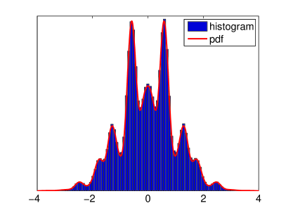
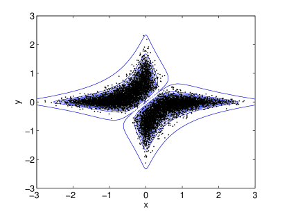
Figure 3 demonstrates our algorithm. Figure 3 (left) shows a histogram of one hundred thousand pseudo-random samples generated from the multimodal density, and Figure 3 (right) shows ten thousand pseudo-random samples from the butterfly density.


We observe that the inverse transform sampling approach described in Section 2 significantly outperforms the Matlab implementation of slice sampling in 1D. In the worst case, the computational cost is comparable to rejection sampling, and in two of the examples it outperforms rejection sampling by a factor of 10.


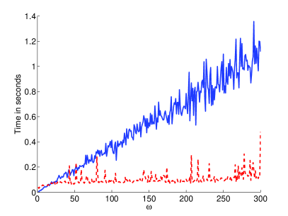
Rejection sampling has practical limitations that inverse sampling avoids. Finding the exact maximum of the distribution for the rejection sampling is computationally expensive, and replacing the exact maximum with a less accurate upper bound causes more samples to be rejected, which reduces its efficiency. Furthermore, the computational cost of each sample is not bounded, and to emphasize this we consider generating pseudo-random samples from for varying on the interval . For large the percentage of the rectangular hat functions area that is under the probability distribution is small, and the rejection sampling approach rejects a significant proportion of its samples, while for our approach the dominating computational cost stays roughly constant. In Figure 4 (left) we compare the computational cost of rejection sampling and the approach described in Section 2, and we observe that the Chebyshev expansion outperforms rejection sampling for .
Remark 2
Of course, for a particular probability distribution a better hat function may be known, which would improve the efficiency of rejection sampling. However, in general accurate hat functions are not available and a rectangular hat function with a known upper bound is the practical choice.
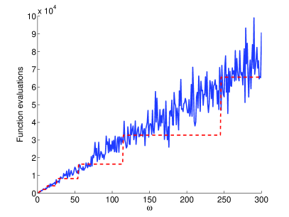
In many applications, the actual evaluation of the probability distribution is expensive. In such circumstances, another benefit of using polynomial approximation in the inverse transform sampling method is that once an approximation has been calculated the original distribution can be discarded, whereas rejection sampling evaluates the original distribution several times per sample. Thus, in Figure 4, we compare the number of function evaluations required to generate samples using rejection sampling versus the number of evaluations for our inverse transform sampling approach. The number of function evaluations are comparable at 50 samples, and hence if 500 pseudo-random samples were required then the rejection sampling approach would require about ten times the number of function evaluations.
Parallelization of the algorithm is important for extremely large sample sizes. This is easily accomplished using a polynomial approximation since the parameters used to represent the CDF can be stored in local memory and the task of generating pseudo-random samples can be divided up among an arbitrary number of processors or machines. However, the rejection sampling approach cannot be parallelized with a black box distribution because evaluation would cause memory locking.
5 Conclusions
We have shown that inverse transform sampling is efficient when employed with Chebyshev polynomial approximation in one dimension, and with low rank function approximation in two dimensions. This allows for an automated and robust algorithm for generating pseudo-random samples from a large class of probability distributions. Furthermore, the approach that we have described can be generalized to higher dimensions by exploiting low rank approximations of tensors.
In fact, the inverse transform sampling approach is efficient for any class of probability distributions that can be numerically approximated, evaluated, and integrated. Therefore, there are straightforward extensions to several other classes of distributions of one variable:
-
1.
Piecewise smooth probability distributions, utilizing piecewise polynomial approximation schemes and automatic edge detection Pachon_10_01 ,
-
2.
Probability distribution functions with algebraic endpoint singularities,
-
3.
Probability distributions with only algebraic decay at , by mapping to a bounded interval via .
The software package Chebfun Chebfun implements each of these special cases.
In two dimensions and higher, approximating general piecewise smooth functions is a more difficult problem, and many fundamental algorithmic issues remain. However, if these constructive approximation questions are resolved the inverse transform sampling approach will be immediately applicable.
References
- (1) M. Bebendorf, Hierarchical Matrices: A Means to Efficiently Solve Elliptic Boundary Value Problems, Volume 63 of Lecture Notes in Computational Science and Engineering (LNCSE). Springer–Verlag, 2008.
- (2) R. P. Brent, Algorithms for Minimization without Derivatives, Englewood Cliffs, NJ: Prentice–Hall, 1973.
- (3) C. W. Clenshaw, A note on the summation of Chebyshev series, Maths Comp., 9 (1955), pp. 118–110.
- (4) C. W. Clenshaw and A. R. Curtis, A method for numerical integration on an automatic computer, Numerische Mathematik, 2 (1960), pp. 197–205.
- (5) P. Deift, Orthogonal Polynomials and Random Matrices: a Riemann–Hilbert Approach, AMS, 2000.
- (6) J. E. Gentle, Random Number Generation and Monte Carlo Methods, Springer, 2003.
- (7) W. R. Gilks, Derivative-free adaptive rejection sampling for Gibbs sampling, In Bayesian Statistics (J. M. Bernardo, J. O. Berger, A. P. Dawid, and A. F. M. Smith, eds.), Oxford Univ. Press, (1992), pp. 641–649.
- (8) W. R. Gilks and P. Wild, Adaptive rejection sampling for Gibbs sampling, Appl. Statist. 41 (1992) pp. 337–348.
- (9) G. H. Givens and J. A. Hoeting, Computational Statistics, 2nd Edition, Wiley, 2013.
- (10) G. Marsaglia and W. W. Tsang, The ziggurat method for generating random variables, J. Stat. Soft., 5 (2000) pp. 1–7.
- (11) J. C. Mason and D. C. Handscomb, The Chebyshev Polynomials, CRC Press, 2003.
- (12) N. Metropolis, A. W. Rosenbluth, M. N. Rosenbluth, A. H. Teller, and E. Teller, Equations of state calculations by fast computing machines, J. Chem. Phys. 21 (1953), pp. 1087–1092.
- (13) R. M. Neal, Slice Sampling, Annals Stats, 31 (2003), pp. 705–741.
- (14) S. Olver and A. Townsend, Inverse Transform Sampling Matlab Implementation, https://github.com/dlfivefifty/InverseTransformSampling.
- (15) R. Pachón, R. B. Platte, and L. N. Trefethen, Piecewise-smooth chebfuns, IMA J. Numer. Anal., 30 (2010), pp. 898–916.
- (16) R. B. Platte, L. N. Trefethen, and A. B. J. Kuijlaars, Impossibility of fast stable approximation of analytic functions from equispaced samples, SIAM Review, 53 (2011) pp. 308–318.
- (17) H. Tanizaki, Computational Methods in Statistics and Econometrics, CRC PressI Llc, 2004.
- (18) A. Townsend and L. N. Trefethen, Gaussian elimination as an iterative algorithm, SIAM News, March 2013.
- (19) A. Townsend and L. N. Trefethen, An extension of Chebfun to two dimensions, (2013), submitted.
- (20) L. N. Trefethen, Approximation Theory and Approximation Practice, SIAM, 2013.
- (21) L. N. Trefethen et al., Chebfun Version 4.2, The Chebfun Development Team, (2011), http://www.maths.ox.ac.uk/chebfun/.
- (22) D. S. Wilks, Statistical Methods in the Atmospheric Sciences, Academic Press, 2011.