Hearing the Shape of the Ising Model with a
Programmable Superconducting-Flux Annealer

Abstract

Two objects can be distinguished if they have different measurable properties. Thus, distinguishability depends on the Physics of the objects. In considering graphs, we revisit the Ising model as a framework to define physically meaningful spectral invariants. In this context, we introduce a family of refinements of the classical spectrum and consider the quantum partition function. We demonstrate that the energy spectrum of the quantum Ising Hamiltonian is a stronger invariant than the classical one without refinements. For the purpose of implementing the related physical systems, we perform experiments on a programmable annealer with superconducting flux technology. Departing from the paradigm of adiabatic computation, we take advantage of a noisy evolution of the device to generate statistics of low energy states. The graphs considered in the experiments have the same classical partition functions, but different quantum spectra. The data obtained from the annealer distinguish non-isomorphic graphs via information contained in the classical refinements of the functions but not via the differences in the quantum spectra.

I Introduction

Kac’s Kak66 question “Can one hear the shape of a drum?” is part of the scientific pop culture Wiki . The technical side of the question concerns our ability to completely specify the geometry of a domain from the eigenvalues of its Laplacian. The question has been reinterpreted in the study of Schrödinger operators on metric graphs by Gutkin and Smilansky Gutkin01 and restated in Algebraic Graphs Theory as “Which graphs are determined by their spectrum?” by van Dam and Haemers vanDam03 . (Through this work, the spectrum of a matrix $M$, denoted by $S_{M}$, is the set of its eigenvalues.) While we commonly employ different types of matrices to encode the structure of graphs, none has yet been shown to efficiently provide a complete graph invariant, i.e., a parameter that does not change under a permutation of the vertex labels. The spectrum of the adjacency matrix, for example, is a common invariant and easily seen to satisfy the “if” part of this statement; however, it is not a complete invariant, given the fact that co-spectral non-isomorphic graphs are abundant Godsil82a ; Godsil82b (see for instance Supplementary Information Section A). In the same spirit, physical scenarios have suggested various notions of refined spectra as a tool for distinguishing graphs, with partial degrees of success Audenaert07a ; Audenaert07b ; Audenaert07b . A common intersection for these approaches is Quantum Mechanics, arguably due to the popularization of quantum dynamics on graphs at the beginning of the last decade Konno08 .

It is interesting, not only from the historical point of view, to observe that the strong link between Physics and graphs is via the Ising model, perhaps the most studied model in Statistical Mechanics. Originally proposed in 1925 Ising25 as a simplified description of the magnetic properties of materials, the Ising model has found a vast number of applications from Biology to Solid State Physics. Its great importance is emphasized by exact solutions and numerical techniques for the identification of phase transitions and critical phenomena Huang90 . The Ising model framework seems particularly suitable to observe differences between Classical and Quantum Mechanics in terms of spectral information, since the quantum case is directly obtained by adding an appropriate (transverse) magnetic field to the classical Hamiltonian.

In what follows, we map a graph into an Ising model and interpret its energy spectrum as a graph invariant, before and after the “switch” from Classical to Quantum Mechanics. We demonstrate with exhaustive numerical examples that the quantum spectrum is a stronger invariant and propose a general framework to define physically meaningful graph polynomials. Determining whether the quantum energy spectrum is a complete invariant remains an open problem. We perform experiments on a programmable annealer with superconducting flux technology Johnson10 . Our purpose is to “hear the shape of an Ising model”, by generating statistics of low energy states as the outcome of a noisy evolution. The experiment is run disregarding whether or not the state of the device follows an adiabatic path along its instantaneous ground state, therefore against the prescription for successful annealing Santoro92 . In other words, we are not only interested in the ground state but, unconventionally, in the full output of a noisy computation. We obtain data on non-isomorphic graphs that are distinguished by their quantum energy spectra but not by the classical ones.

II Results

Classical Cospectrality and Ising models. The Hamiltonian of the Ising model Cipra87 (or, equivalent, $2$-state Potts model) on a graph $G$, with $n$ vertices $V(G)$ and edges $E(G)$, is defined by the diagonal matrix

$$H(G,J):=J\sum_{\{i,j\}\in E(G)}H(i,j)\equiv J\sum_{\{i,j\}}[A(G)]_{i,j}H(i,j)$$ (1)

where, for each edge $\{i,j\}$, $H(i,j):=\bigotimes_{k=1}^{n}H(k)$ is a $2^{n}\times 2^{n}$ matrix, with $H(k)=\sigma_{z}$ if $k=i,j$ and $H(k)=I$, otherwise. $A(G)$ is the adjacency matrix with $[A(G)]_{i,j}=1$ if $\{i,j\}\in E(G)$ and $[A(G)]_{i,j}=0$, otherwise. $\sigma_{z}$ is the Pauli matrix in the $z$-th coordinate axis, $I$ is the identity matrix, and $J$ is the strength of interaction. From now on, whenever the interaction strength is not expressly indicated as, e.g., in $H(G)$, we implicitly set $J=1$ for all edges. The partition function of the Ising model on $G$ is

$$Z(G,v)=\mathrm{Tr}(e^{-\beta H(G)}),$$ (2)

where $\beta:=(k_{B}T)^{-1}$ and $v=e^{\beta J}-1$; $k_{B}$ is Boltzmann’s constant, $T\in\mathbb{R}^{\geq 0}$ is the temperature. By the Fortuin-Kasteleyn Fortuin72 combinatorial identity, $Z(G,v)$ is an evaluation of the Tutte polynomial Tutte54a ; Tutte54b , which is a fundamental invariant that determines many parameters including girth, chromatic number, etc. Remarkably, the Jones polynomial of a knot is contained in the Tutte polynomial Welsch93 . Recall that, formally, $G$ and $G^{\prime}$ are isomorphic if they are the same graph up to a relabeling of the vertices. This is denoted by $G\cong G^{\prime}$. It is not hard to find graphs with the same Tutte polynomial (T-equivalent) that are not isomorphic Mier04a ; Mier04b : for example, all trees on the same number of vertices.

Observe that two graphs $G$ and $G^{\prime}$ have the same partition function if and only if they share the same spectrum of the Hamiltonian in Eq. (1) (i.e. $Z(G,v)=Z(G^{\prime},v)\Leftrightarrow S_{H(G)}=S_{H(G^{\prime})}$). We say that $G$ and $G^{\prime}$ are co-Ising if $S_{H(G)}=S_{H(G^{\prime})}$. Since the Tutte polynomial is a generalization of the partition function, if two graphs are T-equivalent then they share the same energy spectrum and thus are co-Ising. Thus, we know the following:

$$G\cong G^{\prime}\Rightarrow S_{H(G)}=S_{H(G^{\prime})}$$

$$S_{H(G)}=S_{H(G^{\prime})}\nRightarrow G\cong G^{\prime}.$$ (3)

Intuitively, we may attempt a refinement by adding a longitudinal field. The Hamiltonian of the Ising model on $G$ with longitudinal field is defined by the diagonal matrix

$$H_{L}(G,J,h):=H(G,J)+hM,$$ (4)

where $M:=\sum_{i=1}^{n}K(i)$ is a $2^{n}\times 2^{n}$ matrix, with $K(i)=\bigotimes_{k=1}^{n}H_{L}(k)$, $H_{L}(k)=\sigma_{z}$ if $k=i$ and $H_{L}(k)=I$ otherwise. Physically $hM$ can be interpreted as a constant external magnetic field applied to all vertices. Again, we set $J=1$ and $h=1$ unless they are explicitly indicated. We say that two graphs $G$ and $G^{\prime}$ are longitudinal field co-Ising if $S_{H_{L}(G,J,h)}=S_{H_{L}(G^{\prime},J,h)}$ for all values of $J$ and $h$. The following equation summarizes what we know about graphs with this property (see Supplementary Information Section A and B for examples):

$$\stackrel{{\scriptstyle\forall J,h}}{{S_{H_{L}(G,J,h)}\;=\;S_{H_{L}(G^{\prime},J,h)}}} \Rightarrow\stackrel{{\scriptstyle\forall J}}{{S_{H(G,J)}=S_{H(G^{\prime},J)}}}$$

$$S_{H_{L}(G)}=S_{H_{L}(G^{\prime})} \nLeftrightarrow S_{H(G)}=S_{H(G^{\prime})}$$

$${\forall J,h}\;{S_{H_{L}(G,J,h)}=S_{H_{L}(G^{\prime},J,h)}} \nRightarrow G\cong G^{\prime}.$$ (5)

From the diagonal matrices $H(G)$ and $M$, we can define the energy and magnetization vectors as $\mathbf{e}_{\sigma}(G)=H(G)_{\sigma,\sigma}$ and $\mathbf{m}_{\sigma}=M_{\sigma,\sigma}$, where $\sigma=0,2,...,2^{n}-1$ runs over the classical states of the Ising model on $G$, where $0$ denotes the ground state. With the use of these vectors, the bivariate Ising polynomial is defined as Andren09 :

$$Z(G;x,y)=\sum_{\sigma}x^{\mathbf{e}_{\sigma}(G)}y^{\mathbf{m}_{\sigma}}.$$ (6)

Notice that the spectrum $S_{H_{L}(G,J,h)}$ can be obtained from $Z(G;x,y)$ for all values of the constants $J$ and $h$, since a change in these parameters is just a rescaling of the coefficients $x$ and $y$. The Ising polynomial generalizes the partition function in Eq. (2) because $Z(G,e^{-J\beta},1)=Z(G,e^{J\beta}-1)\,$, encodes the matching polynomial, is related to the van der Waerden polynomial, and is contained in a more general polynomial introduced by Goldberg, Jerrum and Paterson Jerrum03a ; Jerrum03b ; Jerrum03c . The bivariate Ising polynomial in Eq. (6) can be intuitively generalized by working with any physical observable in addition to energy and magnetization. If we denote by $\mathbf{o}_{\sigma}^{k}$ the eigenvalues of a diagonal matrix (or observable) $\Lambda^{k}$, we can then define a multivariate polynomial

$$Z(G;x,y,z_{k})=\sum_{\sigma}x^{\mathbf{e}_{\sigma}(G)}y^{\mathbf{m}_{\sigma}}{\displaystyle\prod\limits_{k}}z_{k}^{\mathbf{o}_{\sigma}^{k}}.$$ (7)

An example is given by the (permutationally invariant) spin-glass order parameter used by Hen and Young Hen12 .

Quantum Cospectrality. The invariants that we have so far considered belong to Classical Physics. We can now move into a quantum mechanical regime by adding a further field. The Hamiltonian of the quantum Ising model on $G$, as proposed by Lieb, Schultz, and Mattis Lieb61 (see also Sachdev99 ) is defined by the matrix

$$H_{T}(G,J,h,\Delta):=H_{L}(G,J,h)+\Delta M_{T},$$ (8)

where $\Delta\in\mathbb{R}$ is a transverse external magnetic field; here $M_{T}:=\sum_{i=1}^{n}T(i)$ is a $2^{n}\times 2^{n}$ matrix, with $T(i)=\bigotimes_{k=1}^{n}H_{T}(k)$, $H_{T}(k)=\sigma_{x}$ if $k=i$ and $H_{T}(k)=I$ otherwise. As in the longitudinal case, $M_{T}$ does not depend on $G$. Two graphs $G$ and $G^{\prime}$ are said to be quantum co-Ising if $S_{H_{T}(G,J,h,\Delta)}=S_{H_{T}(G^{\prime},J,h,\Delta)}$ for all values of $J$, $h$ and $\Delta$. It follows from the definition that two graphs are quantum co-Ising if they are isomorphic. The quantum partition function is defined analogously to the classical one:

$$Z_{T}(G,\beta,J,h,\Delta)=\mathrm{Tr}(e^{-\beta H_{T}(G,J,h,\Delta)}).$$ (9)

Two graphs are quantum co-Ising if and only if they have the same quantum partition function. The “if” part of this statement comes directly from the definition. For the “only if” part, observe that in the limit $\beta\rightarrow\infty$, $Z_{T}(G)\simeq\nu_{0}e^{-\beta E_{0}}$ determines the lowest eigenvalue $E_{0}$ with its multiplicity $\nu_{0}$. Similarly, in the same limit $Z_{T}(G)e^{\beta E_{0}}/\nu_{0}$ determines the value and multiplicity of the second smallest eigenvalue. The whole spectrum is obtained iteratively. The statement above and its proof are valid only for systems of finite size. It is a well-known fact that different Hamiltonians can have the same partition function in the thermodynamic limit.

We tested numerically the converse of this fact by computing the smallest eigenvalue for $h=J=\Delta=1$. We tested all graphs with $n\leq 9$, all bipartite graphs with $n\leq 11$, all vertex transitive graphs with $n\leq 15$, all regular graphs with $n\leq 11$, and all trees with $n\leq 14$ (also considered in Andren09 ). We failed to find a counterexample. Hence,

$$G\cong G^{\prime}\Rightarrow S_{H_{T}(G)}=S_{H_{T}(G^{\prime})}$$

$$S_{H_{T}(G)}=S_{H_{T}(G^{\prime})}\overset{?}{\Rightarrow}G\cong G^{\prime}.$$ (10)

The transverse field Ising Hamiltonian is a sum of non-commuting terms and determining its full spectrum requires the diagonalization of a $2^{n}\times 2^{n}$ matrix. We cannot generalize directly the quantum partition function to a generating Ising polynomial as done in the classical case – when eigenvalues are integers (for $J=h=1$) – although we can use the well-known Suzuki-Trotter formalism to obtain a classical approximation Dutta ; the direct calculation of the eigenvalues is notoriously expensive, due to the size of the problem, and prone to errors, making it difficult to numerically show the existence of non-isomorphic quantum co-Ising graphs. A reasonable first approximation for this task is to compute the absolute largest eigenvalue. That is what we have done in our tests. Taking into account such difficulties, finding non-isomorphic quantum co-Ising graphs is an open problem. Natural candidates are graphs for which isomorphism testing is known to be harder to solve (e.g., graphs for which the Weisfeiler-Lehman algorithm fails) Arvind05 . Nevertheless, we emphasize that spectral information provided by Quantum Mechanics is more accurate than Classical Mechanics. It must be said that there are only a few precise (and in fact negative) statements about the physically inspired graph invariants which have been introduced recently (see Audenaert07a ; Audenaert07b ; Audenaert07c ; Hen12 and the references therein) and that purely numerical analysis does not guarantee sufficient generality.

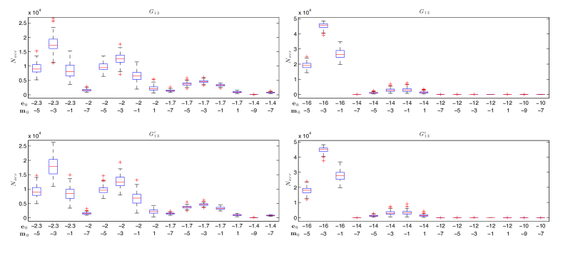
Figure 1: The statistical distribution of measurement outcomes $N_{occ}$ on the pairs $\{G_{13},G_{13}^{\prime}\}$ obtained by averaging over $100$ cycles for each of the $100$ different embeddings considered ($10000$ programming cycles in total). The horizontal red line corresponds to the median of the data while the edges of the blue boxes correspond to the $1$st and $3$rd quartile. Each red cross is an outlier measurement. The outcomes have been filtered after choosing the pair of classical observables {$\mathbf{e}_{0}$, $\mathbf{m}_{0}$}. Data showed in the left panels correspond to the choice $J=h=1/7$. In the right panels $J=h=1$, that is the maximum strength of the couplings allowed by the hardware. With the given choice of classical observables, the distribution of measurement outcomes is not able to distinguish the two graphs, nor at the classical, neither at the quantum level.

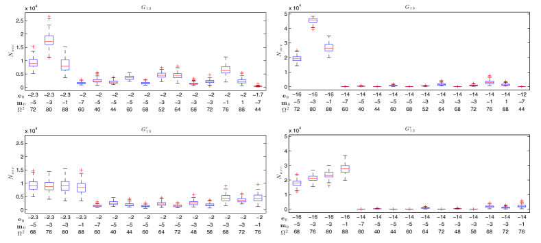
Figure 2: The statistical distribution of measurement outcomes $N_{occ}$ on the pairs $\{G_{13},G_{13}^{\prime}\}$. The outcomes have been now filtered after choosing a triplet of classical observables {$\mathbf{e}_{0}$, $\mathbf{m}_{0}$, $\Omega^{2}$}. Data showed in the left panels correspond to the choice $J=h=1/7$. In the right panels $J=h=1$. Using a third observable distinguishes the two graphs at the classical level.

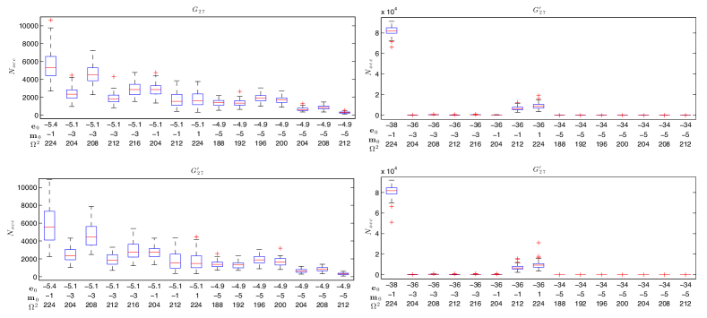
Figure 3: The statistical distribution of measurement outcomes $N_{occ}$ for the pairs $\{G_{27},G_{27}^{\prime}\}$. $J=h=1/7$ in the left panels. $J=h=1$ in the right panels. Filtering the outcomes after choosing the triplet {$\mathbf{e}_{0}$, $\mathbf{m}_{0}$, $\Omega^{2}$} does not distinguishes the graphs at the classical level, and the introduction of additional observables is needed. The shape of the two distributions is also the same, meaning that the two graphs are not distinguished at the quantum level either.

Experiments. Disregarding computational complexity aspects, we have highlighted that from the theoretical point of view one can hear the shape of certain quantum Ising models, while it is not possible for the classical analogue. We subsequently encode on the same physical system pairs of non-isomorphic graphs that are co-spectral, longitudinal field co-Ising (and consequently co-Ising), but not quantum co-Ising. Rather remarkably, our set up finds an experimental implementation in the optimization technique called quantum annealing Finnila ; Kadowaki ; Brooke99 ; Santoro92 . In this technique, the system evolves adiabatically according to the following time-dependent Hamiltonian

$$H_{QA}(G,J,h,\Delta,s)=sH_{L}(G,J,h)+(1-s)\Delta M_{T},$$ (11)

where $s=t/T_{tot}$; $t$ is a time parameter and $T_{tot}$ is the total duration of the dynamics. At the beginning of the computation, the system is prepared in the ground state of the initial simple Hamiltonian $H_{QA}(G,J,h,\Delta,0)=\Delta M_{T}$. On the basis of the adiabatic theorem Farhi00 , adiabatic quantum annealing with general Hamiltonians has been shown to be a universal model of computation by Aharonov et al. Aharonov07 . In synthesis, the core idea is to evolve the system slowly enough towards a final ground state, which is the solution of a computational task. While the success of this paradigm depends on the ability of avoiding level crossings with ad hoc annealing schedules, Brooke et al. Brooke99 experimentally observed that tunneling can hasten convergence to the solution.

In the setting specified by Eq. (11), we are interested in measuring the observables $\mathbf{e}_{0}$, $\mathbf{m}_{0}$, and $\mathbf{o}_{0}^{k}$. In a realistic situation, temperature and environment will usually excite the system. While these effects are disruptive in the standard applications of quantum annealing, we regard such a non-ideal implementation as a way to generate the statistics of low energy states on which we measure the corresponding observables. For this purpose, we run experiments on a D-Wave Vesuvius programmable annealer. The hardware consists of $503$ usable logical bits on an integrated circuit with superconducting flux qubits (see Johnson10 for details on the technology). Quantum effects on the chip are currently under investigation and there is evidence of quantum annealing on random spin glass problems Boixo12a ; Boixo12b ; SSSVa ; SSSVb ; Vinci . The Hamiltonians that can be realized with the device are exactly of the type in Eq. (11), where $s$ is a non-linear function of time. The most general form of the final Hamiltonian $H_{L}$ is given by an Ising model whose possible spin interactions are constrained by the chip architecture. A particular limitation of the hardware is that measurements can be performed only at the end of the evolution. Thus, the maximal information that we can extract is encoded in the multivariate polynomials of Eq. (7). On the other hand, the final state of the chip is a result of a dynamics also governed by the transversal field $M_{T}$. In fact, our experiments attempt to identify the effects of $M_{T}$ in the final statistics after the measurement outcomes are filtered out using various type of multivariate polynomials.

We have tested the annealer on two pairs of non-isomorphic graphs $G$ and $G^{\prime}$ ($G_{13}$ and $G_{13}^{\prime}$, $G_{27}$ and $G_{27^{\prime}}^{\prime}$, in Supplementary Information Section B and C) such that $S_{A(G)}=S_{A(G^{\prime})}$, $S_{H_{L}(G,J,h)}=S_{H_{L}(G^{\prime},J,h)}$, and $S_{H_{T}(G)}\neq S_{H_{T}(G^{\prime})}$, i.e., with equal spectra of the adjacency matrix, equal classical spectra, even with a longitudinal field, and different quantum spectra. To illustrate a possible (arbitrary) refinement as introduced by Eq. (7), we include an extra observable, $\Omega^{2}$, corresponding to the next-nearest neighbor interaction energy: $\Omega^{k}=\sum_{i,j}H(i,j)[A^{k}(G)]_{i,j}$. Notice that $H(G)=\Omega^{1}/2$. Figure 1 shows the statistics of measurement outcomes when the states are distinguished through the doublet of observables {energy, magnetization} on the pairs $\{G_{13},G_{13}^{\prime}\}$, for $J=h=1/7$ and $J=h=1$. These are respectively the smallest and the largest values that can be reliably set on the hardware. The final states are organized according to the values of the two observables. As a consequence of the fact that the two graphs are co-Ising, the measured values of the pairs {energy, magnetization} are the same, and cannot be used to distinguish the two graphs. Moreover, the shape of the two distributions is also the same up to statistical errors. The shape of this distribution is assumed to be a consequence of (noisy) open system quantum dynamics Boixo12a ; Boixo12b (see Supplementary Information Section D for a comparison between experimental and thermal statistics). This means that we are not able to identify differences in the final distributions that may arise due to the different quantum spectra, i.e. due to non-equivalent quantum evolution along the annealing schedule.

The graphs are indistinguishable by measuring energy and magnetization only. However, they become distinguishable in Figure 2 by measuring the triplet {energy, magnetization, $\Omega^{2}$}, as clearly visible in the statistics obtained with the chip. The pair $\{G_{27},G_{27}^{\prime}\}$ is not distinguished by the triplet on the experimental data, as showed in Figure 3. It should be possible, in principle, to classically distinguish these graphs with the introduction of additional observables. Similarly to what happens for the $G_{13}$ pair, there are no noticeable differences in the shape of the final distributions that can detect differences in the quantum spectra.

III Conclusions

The interplay between combinatorics and the classical Ising model is well-established. We have introduced a general family of physically meaningful graph polynomials suggesting a hierarchy of graph invariants. We have demonstrated that the quantum Ising model is a finer sieve to distinguish graphs than its classical analogue by considering the quantum partition function as a graph invariant. We have tested experimentally its distinguishability power on a D-Wave programmable annealer, by taking graphs with different quantum spectra and the same classical Ising partition function. We used the hardware unconventionally to generate the statistics of low energy eigenvalues rather than focusing on the ground state. The data obtained can distinguish one pair of graphs when measuring with respect to a classical refinement of the partition function. We did not find any measurable difference in the statistics of measurement outcomes of the two pairs that can be related to non-equivalent quantum dynamics. Notice that the transverse field spectra are very similar (Fig. 9 in the Supplementary Material). Of course, differences expected in an ideal quantum system are possibly lost due to decoherence when approaching the classical regime at the end of the adiabatic evolution.

Going beyond the scope of this work, it would be interesting to compare the experimental data with numerical simulations of the corresponding open quantum spin system at finite temperature Albash12 . We propose two approaches to amplify the differences in the quantum spectra: (a) reduce substantially the annealing time; (b) perform measurements when the transverse field is on. Both approaches require a modification of the current control of the hardware. Another interesting goal is to define other efficient observables, such as $\Omega^{2}$, that would amplify the possible differences in the measurement statistics. From the theoretical point of view a natural open question is whether the transverse field alone is sufficient to define a complete spectral graph invariant.

IV Methods

Experimental data collection. In order to collect enough statistics for averaging over biases and systematic errors, we have considered $100$ embeddings in the chip for each graph. To average over precision errors when setting the intended couplings on the machine, we have run $100$ programming cycles for each embedding. For each cycle, we have performed $1000$ measurements. All the experiments have been performed choosing the shortest annealing time allowed by the hardware ($T_{tot}=20\mu s$) in order to minimize the effects of thermal excitations.

V Acknowledgments

We would like to thank Gabriel Aeppli, Andrew Fisher, Andrew Green, Itay Hen, Daniel Lidar, Brent Segal, and Peter Young for valuable discussion. This work has been done within a “Global Engagement for Global Impact” programme funded by EPSRC, and with support from ARO grant number W911NF-12-1-0523, the Lockheed Martin Corporation and DARPA grant number FA8750-13-2-0035.

VI Author Contribution

W.V., S.S. and P.A.W. provided the central ideas, that were further developed by all authors. K.M. performed the numerical exhaustive analysis of the graphs considered in the paper. W.V. performed all data collection and analysis. A.R. contributed in the data collection. S.B. and F.M.S. contributed in the data analysis. W.V. and S.S. wrote the main manuscript text. All authors thoroughly reviewed the final manuscript.

VII Additional Information

Competing financial interests: The authors declare no competing financial interests.

Appendix A Supplementary Material

Appendix B A. Examples for Eq. (II)

The two graphs $G_{1}\ncong G_{2}$ on $7$ vertices with

$$E(G_{1}) =\{1,5;1,7;2,6;2,7;3,7\},$$

$$E(G_{2}) =\{1,5;2,6;2,7;3,6;3,7\},$$ (12)

are such that $S_{H_{L}(G_{1})}=S_{H_{L}(G_{2})}$ and $S_{H(G_{1})}\neq S_{H(G_{2})}$ (see Fig. 4). We note that in general $S_{H_{L}(G_{1},J,h)}\neq S_{H_{L}(G_{2}^{\prime},J,h)}$. The two graphs $G_{3}\ncong G_{4}$ on $4$ vertices with

$$E(G_{3}) =\{1,4;2,4\},$$

$$E(G_{4}) =\{1,3;2,4\},$$ (13)

are such that $S_{H(G_{3})}=S_{H(G_{4})}$ and $S_{H_{L}(G_{3})}\neq S_{H_{L}(G_{4})}$ (see Fig. 5).

Appendix C B. Experiments for $G_{13}$ and $G_{13}^{\prime}$

The two graphs $G_{13}\ncong G_{13}^{\prime}$ on $13$ vertices with

$$E(G_{13}) =\{1,8;1,10;1,11;1,13;2,9;2,11;2,13;3,10;3,13;4,10;5,11;6,12;7,12;9,12;12,13\},$$

$$E(G_{13}^{\prime}) =\{1,8;1,10;1,11;1,13;2,9;2,11;2,13;3,10;3,11;4,10;5,12;6,12;7,13;8,12;12,13\},\$$ (14)

are such that $S_{A(G_{13})}=S_{A(G_{13}^{\prime})}$, $S_{H_{L}(G_{13},J,h)}=S_{H_{L}(G_{13}^{\prime},J,h)}$ and $S_{H_{T}(G_{13})}\neq S_{H_{T}(G_{13}^{\prime})}$ (see Fig. 6). The triplet {energy, magnetization, $\Omega^{2}$} distinguishes $G_{13}$ and $G_{13}^{\prime}$. The measurements performed on the chip distinguish the graphs (see Fig. 1 in the main text). Let $\lambda_{\max}(G)>\lambda_{2^{n}-1}(G)\geq\cdots\geq\lambda_{2}(G)>\lambda_{\min}(G)$ be the eigenvalues of $H_{QA}(G,1,1,1,s)$ as a function of $s$. Fig. 9 shows $\lambda_{i}(G_{13})-\lambda_{\min}(G_{13})$ and $\lambda_{i}(G_{13}^{\prime})-\lambda_{\min}(G_{13}^{\prime})$, for $i=2,...,20$. The similarity between the two spectra is evident.

Fig. 7 contains five embeddings of the graph $G_{13}$ (and $G_{27}$) on the chip. We include this figure to clarify the notion of physically different embeddings of the same graph.

Appendix D C. Experiments for $G_{27}$ and $G_{27}^{\prime}$

Consider the two graphs $G_{27}\ncong G_{27}^{\prime}$ with edges

$$E(G_{27}) =\{1,14;1,17;2,14;2,22;3,4;3,5;4,3;4,10;4,12;5,3;5,11;5,13;6,7;6,8;6,15;$$

$$7,10;7,11;8,13;9,12;9,13;9,14;10,15;11,15;14,15;16,17;16,21;17,18;18,19;$$

$$19,20;20,21;22,23;22,27;23,24;24,25;25,26;26,27\},$$

$$E(G_{27}^{\prime}) =\{1,14;1,17;2,14;2,23;3,4;3,5;4,3;4,10;4,11;5,12;5,13;6,7;6,8;6,15;7,10;$$

$$7,12;8,11;8,13;9,12;9,13;9,14;10,15;11,15;14,15;16,17;16,21;17,18;18,19;$$

$$19,20;20,21;22,23;22,27;23,24;24,25;25,26;26,27\}.$$ (15)

For these graphs, $S_{A(G_{27})}=S_{A(G_{27}^{\prime})}$ and $S_{H_{L}(G_{27},J,h)}=S_{H_{L}(G_{27}^{\prime},J,h)}$ (see Fig. 8). We do not know if $S_{H_{T}(G_{27})}\neq S_{H_{T}(G_{27}^{\prime})}$. We would expect in this case differences in the quantum spectra to be even smaller than those in the case of $G_{13}$ and $G_{13}^{\prime}$. The triplet {energy, magnetization, $\Omega^{2}$} distinguishes $G_{27}$ and $G_{27}^{\prime}$ when considering the full spectrum. However, Fig. 3 shows that the graphs are undistinguishable by the measurements performed on the chip for $J=h=1/7$.

As a check that the data statistics are not critically dependent on the embeddings considered, we show in Fig. 10 the statistics corresponding to half of the embeddings in each case.

Appendix E D. Comparison to Gibbs statistics

To substantiate our assumption that the experimental data are a consequence of a noisy quantum evolution, we have compared the signature distributions to those obtained by sampling from a thermal Gibbs distribution defined on the classical Ising models associated to the graphs. The results are shown in Fig. 11 for the $G_{13}$ graph and two choices of the couplings. The temperature for the Gibbs sampling has been chosen to best reproduce the experimental data. The two distributions are notably different, although they show many qualitative common features.

Figure 4: Graphs $G_{1}$ (left) and $G_{2}$ (right) with $S_{H_{L}(G_{1})}=S_{H_{L}(G_{2})}$ and $S_{H(G_{1})}\neq S_{H(G_{2})}$

Figure 5: Graphs $G_{3}$ (left) and $G_{4}$ (right) with $S_{H(G_{3})}=S_{H(G_{4})}$ and $S_{H_{L}(G_{3})}\neq S_{H_{L}(G_{4})}$.

Figure 6: Graphs $G_{13}$ (left) and $G_{13}^{\prime}$ (right).

Figure 7: The grid in the figure above shows the hardware connectivity. Each circle is a programmable superconducting pseudo spin, while the connecting lines represent the physical interactions that can be implemented in the chip. The black circles and lines correspond to the “active” part of the hardware that is used to implement five example embeddings of $G_{13}$ (left) and $G_{27}$ (right) on the chip.

Figure 8: Graphs $G_{27}$ (left) and $G_{27}^{\prime}$ (right).

Figure 9: Quantum spectra $\lambda_{i}$ of $H_{QA}(G_{13},1,1,1,s)$ (solid line) and $H_{QA}(G_{13}^{\prime},1,1,1,s)$ (dotted line) as a function of $s$.

Figure 10: Average value of measurement outcomes $\langle N_{occ}\rangle$ for each programming cycle for the graphs $G_{13}$ (left) and $G_{27}$ (right). $J=h=1/7$. The statistics corresponding to one half of the embeddings is shown in the red circles and the other half in the blue stars. Error bars have been estimated with a bootstrap technique. We have extracted $5000$ bootstrap samples out of the two halves of the total programming cycles performed (10000).

Figure 11: The figure compares experimental data to thermal Gibbs distributions for the graph $G_{13}$. The left panel corresponds to the upper left panel of Fig. 1 ($J=h=1/7$). The right panel corresponds to the upper right panel of Fig. 1 ($J=h=1$). The temperature to generate the Gibbs sampling has been chosen as the one that reproduces the statistics of the second collection of states. Error bars have been estimated with a bootstrap technique. We have extracted $1000$ bootstrap samples out of $1000$ randomly picked programming cycles. The numerically generated Gibbs statistics contains the same number of generated states ($10^{6}$). We have checked that the error estimates are consistent by repeating the bootstrap sampling.

References

- (1) Kac, M. Can one hear the shape of a drum? The American Mathematical Monthly 73, 1–23 (1966).
- (2) Wikipedia contributors. Hearing the shape of a drum. Wikipedia, The Free Encyclopedia. http://en.wikipedia.org/wiki/Hearing_the_shape_of_a_drum. (24/06/2014).
- (3) Gutkin, B. & Smilansky, U. Can one hear the shape of a graph? J. Phys. A. Math. Gen. 34, 6061–6068 (2001).
- (4) van Dam, E. R. & Haemers, W. H. Which graphs are determined by their spectrum? Linear Algebra Appl. 373, 241–272 (2003).
- (5) Godsil, C. D. & McKay, B. D. Constructing cospectral graphs. Aequationes Math. 25, 257–268 (1982).
- (6) Godsil, C. & Royle, G. Algebraic Graph Theory. (Springer–Verlag, 2001).
- (7) Audenaert, K. et al. Symmetric squares of graphs. J. Comb. Theory, Ser. B 97(1), 74–90 (2007).
- (8) Emms, D. et al. A matrix representation of graphs and its spectrum as a graph invariant. Electron. J. Combin. 13(1), R34 (2006).
- (9) Gamble, J. K., Friesen, M., Zhou, D., Joynt, R. & Coppersmith, S. N. Two–particle quantum walks applied to the graph isomorphism problem. Phys. Rev. A 81, 052313 (2010).
- (10) Konno, N. Quantum walks. Quantum Potential Theory, Lecture Notes in Mathematics, [309–452] (Springer–Verlag, Berlin Heidelberg, 2008).
- (11) Ising, E. Beitrag zur Theorie des Ferromagnetismus. Z. Physik 31, 253–258 (1925).
- (12) Huang, K. Statistical Mechanics. (Wiley, John & Sons, 1990).
- (13) Johnson, M. W. et al. Quantum annealing with manufactured spins. Nature 473, 194198 (2011).
- (14) Santoro, G. E. et al. Theory of Quantum Annealing of an Ising Spin Glass. Science 295, 24272430 (2002).
- (15) Cipra, B. A. An Introduction to the Ising Model. Amer. Math. Monthly 94, 937–959 (1987).
- (16) Fortuin, C. M., Kasteleyn, P. W. On the random cluster model. I. Introduction and relation to other models. Physica 57, 536–564 (1972).
- (17) Tutte, W. T. A contribution to the theory of chromatic polynomials. Canad. J. Math. 6, 80–91 (1954)
- (18) Whitney, H. The coloring of graphs. Ann. Math., 33, 688–718 (1932).
- (19) Welsh, D. J. A. Complexity: knots, colorings and counting, London Mathematical Society Lecture Note Series 186. (Cambridge University Press, Cambridge, 1993).
- (20) de Mier, A. & Noy, M. On graphs determined by their Tutte polynomial. Graph. Comb. 20, 105–119 1 (2004).
- (21) Garijo, D., Goodall, A. & Nešetřil, J. Distinguishing graphs by their left and right homomorphism profiles. Eur. J. Comb. 32, 1025–1053 (2011).
- (22) Andren D. & Markstrom, K. The bivariate Ising polynomial of a graph. Discrete Appl. Math. 157(11), 2515–2524 (2009).
- (23) Goldberg, L. A., Jerrum, M., Paterson, M. The computational complexity of two-state spin systems. Random Struct. Alg. 23, 133–154 (2003).
- (24) Kotek, T. Complexity of Ising polynomials. Combin. Probab. Comput. 21, 743–772 (2012).
- (25) van der Waerden, B. L. Die lange reichweite der regelmassigen atomanordnung in mischkristallen. Zeitschrift für Physik 118, 573–479 (1941).
- (26) Hen I., & Young, A. P. Solving the graph-isomorphism problem with a quantum annealer. Phys. Rev. A 86, 042310 (2012).
- (27) Lieb, E., Schultz, T. & Mattis, D. Two soluble models of an antiferromagnetic chain. Ann. Phys., 16, 407–466 (1961).
- (28) Sachdev, S. Quantum Phase Transitions. (Cambridge University Press, Cambridge, 1999).
- (29) Dutta, A. et al. Quantum phase transitions in transverse field spin models: From Statistical Physics to Quantum Information. arXiv:1012.0653
- (30) Arvind, V. & Torán, J. Isomorphism Testing: Perspective and Open Problems. Bulletin of the EATCS 86, 66–84 (2005).
- (31) Brooke, et al. J. Quantum Annealing of a Disordered Magnet. Science 284, 779781 (1999).
- (32) Finnila, A. et al. Quantum annealing: a new method for minimizing multidimensional functions. Chem. Phys. Lett., 219, 343–348 (1994).
- (33) Kadowaki, T. & Nishimori, H. Quantum annealing in the transverse Ising model. Phys. Rev. E 58, 5355–5363 (1998).
- (34) Farhi, E. et al. Quantum Computation by Adiabatic Evolution. arXiv:quant-ph/0001106.
- (35) Aharonov, D. et al. Adiabatic Quantum Computation is Equivalent to Standard Quantum Computation. SIAM J. Comput. 37, 166 (2007).
- (36) Boixo, S. et al. Experimental signature of programmable quantum annealing. Nature Comm. 4, 3067 (2013)
- (37) Boixo, S. et al. Evidence for quantum annealing with more than one hundred qubits. Nature Physics 10, 218 (2014).
- (38) Smolin, J. A. & Smith, S. Classical signature of quantum annealing. arXiv:1305.4904
- (39) Shin, S. W. et al. How ”Quantum” is the D-Wave Machine? arXiv:1401.7087.
- (40) Vinci, W. et al. Distinguishing Classical and Quantum Models for the D-Wave Device. arXiv:1403.4228.
- (41) Albash, T. et al. Quantum adiabatic Markovian master equations. New J. Phys. 14, 123016 (2012).