Flavor Model in Three Loop Seesaw and Higgs Phenomenology
Abstract
We propose a new type of radiative seesaw model in which observed neutrino masses are generated through a three-loop level diagram in combination with tree-level type-II seesaw mechanism in a renormalizable theory. We introduce a Non-abelian flavor symmetry in order to constrain the form of Yukawa interactions and Higgs potential. Although several models based on a Non-abelian flavor symmetry predict the universal coupling constants among the standard model like Higgs boson and charged leptons, which is disfavored by the current LHC data, our model can avoid such a situation. We show a benchmark parameter set that is consistent with the current experimental data, and we discuss multi-muon events as a key collider signature to probe our model.
I Introduction
A new boson has been discovered at Large Hadron Collider (LHC), whose properties of the production and decay are consistent with those of the Higgs boson in the standard model (SM) ATLAS_Higgs ; CMS_Higgs . This fact, the observed particle is the SM-like Higgs boson (), could seriously affect to models for the charged lepton with flavor symmetries Ishimori:2012zz ; Ishimori:2010au ; Altarelli:2010gt , since some models could be ruled out. As a typical example, we show models based on Non-abelian discrete symmetries such as 111The flavor symmetry was initially applied to the lepton sector in Ref. Babu:2002dz ; Ma:2001dn , in which the structure of the charged lepton does not have the universal coupling. However Ferreira:2013oga has those., Luhn:2007sy , Ma:2007wu ; Ma:2006ip , Ishimori:2012gv ; Ma:2006ht , that only have the irreducible representations of singlets (typically introduced as Higgs fields) and triplets (typically as leptons). The Lagrangian is then given by
| (I.1) |
where , and are the isospin Higgs doublet, isospin lepton doublet and isospin lepton singlet fields, respectively, and . The mass matrix for the charged leptons are then calculated from Eq. (I.1) as
| (I.2) |
where . By solving Eq. (I.2), the Yukawa couplings can be derived as
| (I.3) |
Although the Lagrangian shown in Eq. (I.1) gives the simple structure for the generation of the charged lepton masses as we see in Eqs. (I.2) and (I.3), this results that all the coupling constants among the charged leptons and the CP-even scalar component of are determined by the same Yukawa coupling . That makes the branching fractions of , and modes to be the same with each other, where is the mass eigenstate of the CP-even states with the mass of 126 GeV identified to any of . Such a situation is extremely disfavored by the current results of the Higgs boson search at LHC, namely, the event rate for is almost the same as that in the SM, while the event of has not been observed yet222From the current LHC data, has been excluded at 95 confidence level dimuon ..
In the present paper, we clarify the relation between the lepton sector and the Higgs sector in the flavor symmetry Ishimori:2012sw ; Cao:2011cp ; Cao:2010mp ; Hagedorn:2008bc . As for the neutrino sector, two mechanisms of type-II seesaw typeII and radiative seesaw with several loops333 As for the other radiative seesaw models, see Refs. zee-babu ; Kajiyama:2013zla ; Ma:2006km ; Sahu ; Aoki:2013gzs ; Krauss:2002px ; Aoki:2008av ; Schmidt:2012yg ; Bouchand:2012dx ; Ma:2012ez ; Aoki:2011he ; Ahn:2012cg ; Farzan:2012sa ; Bonnet:2012kz ; Kumericki:2012bf ; Kumericki:2012bh ; Ma:2012if ; Gil:2012ya ; Okada:2012np ; Hehn:2012kz ; Dev:2012sg ; Kajiyama:2012xg ; Okada:2012sp ; Aoki:2010ib ; Kanemura:2011vm ; Lindner:2011it ; Kanemura:2011mw1 ; Kanemura:2011mw2 ; Kanemura_Sugiyama ; Gu:2007ug ; Gu:2008zf ; Gustafsson ; two-triplet ; Kanemura:2013qva ; Law:2013saa . are involved to induce the neutrino observables. Especially, our scenario requires up to a specific three-loop diagram that gives diagonal components to neutrino mass matrix, while the off-diagonal components are obtained through the type-II seesaw mechanism at tree level. As for the Higgs sector, we consider the whole Higgs potential and derive all the masses of the Higgs bosons. We then analyze the behavior of the SM-like Higgs boson, by fixing a benchmark point. Our analyses of the Higgs fields could be applied to many models, e.g. lepton flavor models with Non-abelian discrete symmetries. Since the Higgs sector in the present model is similar to that of the Type-X or lepton specific two Higgs doublet model (THDM) typeX ; typeX2 , constraints from hadron collider experiments are rather weak. We give a numerical example, in which decay modes of the second lightest CP-odd, -even and charged Higgs bosons are mainly muons. This will be signals of the present model.
This paper is organized as follows. In Section 2, we show particle contents of our model, and discuss Higgs boson masses and neutrino masses generated at tree and three- loop level. In Section 3, we analyze phenomenology of Higgs bosons. We summarize and conclude in Section 4. In appendices, some results of detailed calculations for the Higgs sector and radiatively induced neutrino masses are given.
II Three Loop Radiative Seesaw Model
In this section, we propose a three-loop radiative seesaw model which is an extension of the minimal Higgs triplet model motivated from the type-II seesaw mechanism typeII . First, we give particle contents and Yukawa interactions. After that, masses for the Higgs bosons and neutrinos are discussed.
II.1 Model setup
| Particle | |||||||||
The particle contents are shown in Tab. 1. We add three triplet scalar fields , three doublet scalar fields , (), and an doublet scalar field , where do not have the vacuum expectation values (VEVs). The parity is imposed so as to forbid terms such as . The parity is introduced in order to avoid couplings among and leptons. The renormalizable Lagrangian of Yukawa interactions is given by
| (II.1) | ||||
| (II.2) | ||||
| (II.3) |
Four doublet Higgs fields and three triplet Higgs fields can be parameterized as
| (II.8) | ||||
| (II.11) |
where and are the VEVs for the doublet fields and are those for the triplet fields, which satisfy the sum relation
| (II.12) |
The VEVs of the doublet Higgs fields are related to the charged lepton mass matrix from Eq. (II.1) as
| (II.13) |
which is already diagonal and has the common Yukawa coupling due to symmetry. Mass hierarchy between charged leptons should be explained by the hierarchy of VEVs. We note that the masses of quarks are generated by in the same way as in the SM. On the other hand, the triplet VEVs generate neutrino masses. Non-zero values for the triplet VEVs cause the deviation in the electroweak rho parameter from unity as
| (II.14) |
Because the experimental value of is given as , the triplet VEVs are constrained by to be about (3.8 GeV)2 at the 95% confidence level. Thus, the sum relation given in Eq. (II.12) can be approximately rewritten by
| (II.15) |
The ratio of the above two VEVs can be described as .
II.2 Higgs boson masses
Next, we discuss the Higgs potential, especially for the even scalar sector assuming CP conservation. The invariant Higgs potential is given by
| (II.16) |
where terms with the index should be summed over . In addition to the above terms, we introduce the following soft terms which break the symmetry into symmetry;
| (II.17) |
The potential given in Eqs. (II.16) and (II.17) is not the most general form, where we only write down terms which are relevant to the following phenomenological studies444 Most of terms which are not displayed in Eqs. (II.16) and (II.17) are not important from the following reasons. First, they can contribute to masses for scalar bosons with the magnitude of . Such a contribution can be negligible, because of . Second, they give masses for odd scalar bosons, which are not related to the following discussions. . The complete expressions for the Higgs potential are given in Appendix A. We note that the term is necessary to break an accidental symmetry of the phase rotation , otherwise there exists an additional massless Nambu-Goldstone (NG) boson that cannot be absorbed by a gauge field. It implies that the mass scale of must be GeV at most, since plays an important role in obtaining mass of the lightest CP-odd Higgs boson in Eq. (II.45). The LHC experiment tells us that its mass must be more than 100 GeV as we will discuss in the section III.
From the tadpole condition, we obtain
| (II.18) |
where and .
There are seven (six) physical CP-even (CP-odd) scalar bosons, six pairs of singly-charged scalar bosons and three pairs of the doubly-charged scalar bosons in addition to the neutral and the charged NG bosons which are obtained after the diagonalization and absorbed by the longitudinal component of the and bosons, respectively. The mass matrix for the CP-even Higgs bosons in the basis of is given by
| (II.21) |
where , and are the sub-matrices of , which are , and forms, respectively. They can be expressed as
| (II.26) | ||||
| (II.34) |
where . Similarly, each of the mass matrix for the CP-odd scalar bosons and that for the singly-charged scalar bosons in the basis of and can be expressed by
| (II.39) |
where (), () and () are the sub-matrix for () which are , and , respectively. Each sub-matrix can be obtained as
| (II.44) | ||||
| (II.45) |
and
| (II.50) | ||||
| (II.51) |
One can find that the eigenvectors belonging to the NG modes and are given as
| (II.52) | ||||
| (II.53) |
We can construct the unitary matrices which make and to be the block diagonal forms by using , and those orthogonal vectors, in which the NG modes are decoupled from the physical scalar states. We do not show explicitly these unitary matrices, because their analytic formulae are too complicated to show in the paper.
Under which is required by the rho parameter data, the diagonal elements of become much larger than elements in . In that case, the diagonalization matrices for , and are given as a block diagonal form like and , so that we can separately consider the mass eigenstates which are mainly composed of doublets from those of triplets. We then define the mass eigenstates for the CP-even, CP-odd and singly-charged scalar bosons as follows
| (II.78) |
The masses for the Higgs bosons can be calculated as
| (II.79) | |||
| (II.80) | |||
| (II.81) |
Approximately, the masses for the Higgs bosons can be expressed in the case of as
| (II.82) | |||
| (II.83) | |||
| (II.84) | |||
| (II.85) | |||
| (II.86) |
with
| (II.87) | |||
| (II.88) | |||
| (II.89) | |||
| (II.90) |
In addition, first part of the unitary matrices are written as
| (II.91) | |||
| (II.92) |
We note that is dominantly proportional to , so that should be taken to be as large as TeV and to be of GeV to compensate the tiny triplet VEV. Moreover, if one assumes that the mass of is of TeV, should be at most of TeV, because there is strong correlation between and , , as is often the case with the usual type-II seesaw.
The mass matrix for the doubly-charged scalar states is expressed by the form, because they purely come from the triplet Higgs fields. In the basis of , the mass matrix is the same as given in Eq. (II.34). Their squared mass eigenvalues are typically determined by , so that these are ( TeV)2 as long as we take GeV and TeV.
In the following discussion, we treat as the SM-like Higgs boson which should be identified to be a new boson discovered at LHC with the mass of GeV.
II.3 Neutrino mass matrix

In this subsection, we discuss neutrino masses which are induced at three-loop level as well as at tree level. First, the tree-level mass matrix for neutrinos is given through Eq.(II.3) as
| (II.93) |
When , the Pontecorvo-Maki-Nakagawa-Sakata matrix at the tree level is given by
| (II.94) |
and it diagonalizes as
| (II.95) |
where
| (II.96) |
and the maximal mixing are originated from the condition . However, this condition can be relaxed to obtain non-zero and observed value of at range. As mentioned before, we take to obtain the phenomenologically enough large mass for , so that is required to reproduce . Since there exist only three parameters in Eq. (II.93), one cannot derive all observables in neutrino sector. Therefore, one has to take loop-level mass matrices into account.
Next, we discuss loop level neutrino masses. The tree level mass matrix does not have non-zero diagonal entries and neutrino observables cannot be derived at tree level. Therefore we focus on diagonal elements induced by loop diagrams. To achieve it, we summarize how to generate Majorana neutrino mass matrix by Yukawa interactions given in Eqs. (II.1) and (II.3) as listed in the following:
-
(i) Each attached on the fermion line gives one .
-
(ii) Odd number of s should be attached on the fermion line for lepton number violation.
-
(iii) At least, three s should be attached on the fermion line in order to generate diagonal elements of neutrino mass matrix, because changes the lepton flavor, while does not. If only one is attached, it always gives off-diagonal elements of neutrino mass matrix.
-
(iv) On fermion line between and , chirality suppression occurs.
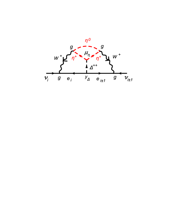
Along these lines of thought, one finds that the sizable contributions to diagonal elements are given at three-loop level shown in Fig. 1, and its magnitude can be estimated as555The exact form is found in Appendix B.
| (II.97) |
where is the dimensionful coupling associated with the invariant term defined in Eq. (II.16), and and are the typical and masses; and , respectively. Notice here that the mass parameter , which is taken to be , contributes only to the masses, since do not mix with and due to the inert property. Hence one can take arbitrarily large value for with no effects to masses of and 666This is, in a sense, a fine-tuning that one has to tune the bare mass of to cancel the large loop contribution from in order to obtain the small physical mass of . This is similar to the renormalization of the Higgs boson mass in the SM if the cutoff scale is assumed to be a large scale such as the grand unification scale or Planck scale. We expect that such a fine-tuning problem may be able to be solved by extending our model to the supersymmetric theory. We would like to thank the referee to draw our attention to such kind of matter.. As a result, we can reproduce observed neutrino masses (0.1) eV and the mixing data because of many parameters, as can be seen in Appendix B. As for the other contributions up to three-loops, see Appendix C.
III Higgs Phenomenologies
In this section, we discuss the collider phenomenology of the Higgs bosons. This model can be effectively regarded as the so-called Type-X or lepton specific THDM typeX ; typeX2 , in which one of the two Higgs doublets couples to quarks and the other one couples to leptons. To see this, we write down the interaction terms in the Yukawa Lagrangian given in Eqs. (II.1) and (II.2) in terms of the mass eigenstates of the Higgs bosons as follows
| (III.1) |
where Sign()=1 () for (), and the projection operators are and . From the above expression, the ratio of the Yukawa coupling in our model to that in the SM, , and the similar rate of the gauge coupling for can be calculated as
| (III.2) |
The SM-like limit, in which the coupling constants of are the same as those in the SM Higgs boson, can be obtained by taking the following limit
| (III.3) |
By using , this limit can also be approximately expressed as which is the same form known in the THDMs with a softly broken discrete symmetry. In the SM-like limit, factors of the vertices among the lightest extra Higgs bosons (, and ) and fermions are calculated by
| (III.4) |
It can be seen from the above expressions that the lepton (quark) couplings can be enhanced (suppressed) in the case with large . This feature in our model is very similar to that of the Type-X THDM.
III.1 Current experimental constraints
We here consider constraints from the current experimental data. As we discussed in the previous subsection, phenomenology of the lightest extra Higgs bosons (, and ) can be regarded as that in the Type-X THDM, so that the current experimental bound can be applied to our model in the similar way as that in the Type-X THDM. We take into account the following constraints.
-
1.
At the LEP direct search experiment, masses for extra CP-odd, CP-even and charged Higgs bosons have been constrained from below by 93.4 GeV, 92.8 GeV and 79.3 GeV, respectively, with the 95% confidence level in supersymmetric (SUSY) models PDG .
-
2.
From the physics experiments, the mass of charged Higgs bosons is strongly constrained in multi-doublet models. For example, from the data, the lower limit of has been given by 295 GeV Misiak with the 95% confidence level in the Type-II THDM with . However, this constraint turns out to be quite weak in the Type-I and Type-X THDMs; i.e., GeV with is allowed with the 95% confidence level as shown in Ref. typeX ; typeX2 ; Stal . The other processes including the meson such as , , etc. give milder bounds compared to that from the process777Recently, BaBar Collaboration has reported data on the ratios and () that deviate from the SM expectations by and , respectively, and their combined deviation is Babar . These deviations cannot be simultaneously explained by the contributions of the charged Higgs boson in the softly-broken symmetric THDMs. in the Type-X THDM.
-
3.
At LHC, the ATLAS and the CMS Collaborations have reported the signal strength for a Higgs boson like particle with the mass of around 126 GeV. So far, five decay modes of the Higgs boson have been mainly analyzed, those are , , , and . Their signal strengths are consistent with the prediction in the SM within the two-sigma level Moriond_ATLAS ; Moriond_CMS . Thus, the parameter regions which give the SM-like limit explained in Eq. (III.3) are also allowed in our model.
-
4.
The extra neutral Higgs bosons in the minimal SUSY SM (MSSM); i.e., the CP-even Higgs boson and the CP-odd Higgs boson have been searched by using the pair decay mode in the gluon fusion process and the bottom quark associated process MSSM_neutral_ATLAS ; MSSM_neutral_CMS by using the data collected at LHC with the collision energy to be 7 TeV. When the mass of the CP-odd Higgs boson is taken to be from 110 GeV to 150 GeV, the 95% confidence level lower limit for has been obtained to be about 10 in Ref. MSSM_neutral_ATLAS . Although the Higgs sector in the MSSM corresponds to the Type-II THDM, this constraint cannot be simply applied to the non-SUSY Type-II THDM due to SUSY relations. Understanding this, let us assume that the 95% confidence level upper limit for the cross section of and is given by these cross sections calculated in the Type-II THDM with the case of , and . The cross section can be calculated by
(III.5) where each of () and () is the cross sections of the and processes with being the SM Higgs boson whose mass is taken to be the same as the mass of . In the Type-X THDM, can be almost 100% when . On the other hand, the quark couplings with and are proportional to , so that the cross section can be the maximal value at around typeX . In Tab. 2, the lower limit for the value of in the Type-X THDM in the case with and is listed, which is obtained by imposing the upper limit for the cross section given in Eq. (III.5). We note that this constraint for can be relaxed when the mass degeneracy in and is not assumed.
-
5.
The charged Higgs boson in the MSSM has been searched from the top quark decay at LHC. In Refs. MSSM_charged_ATLAS ; MSSM_charged_CMS , the excluded regions at the 95% confidence level in the - plane are shown. However, in the Type-X THDM, the decay rate of is suppressed by the factor of typeX ; typeX2 , so that the constraint from the top decay becomes much weaker than that obtained in the MSSM.
| [GeV] | [pb] Higgs_cross | [pb] | [pb] | |
|---|---|---|---|---|
| 110 | 19.8 | 0.212 | 5.60 | 2.5 |
| 120 | 16.7 | 0.155 | 4.00 | 2.9 |
| 130 | 14.2 | 0.116 | 2.93 | 3.2 |
| 140 | 12.2 | 0.089 | 2.20 | 3.6 |
| 150 | 10.6 | 0.068 | 1.67 | 3.8 |
According to the above constraints, we here give an example of the allowed parameter set as
| (III.6) | |||
| (III.7) |
We then obtain the following outputs
| (III.8) | |||
| (III.13) |
| (III.14) | |||
| (III.19) | |||
| (III.20) | |||
| (III.25) |
As it can be seen the value of elements in , this set is one of the realizations of the SM-like limit defined in Eq. (III.3). The masses of the triplet-like Higgs bosons whose components are mainly from the triplet Higgs field (, and ) including the doubly-charged Higgs bosons are around 2-3 TeV. These magnitudes are typical in our model, because the (squared) triplet-like Higgs boson masses are given like as we discussed in the previous section, and () have to be of order 1 TeV (1 GeV) to raise the mass.
Finally, we comment on collider signatures of extra Higgs bosons. Although the existence of the doubly-charged Higgs bosons can be a clear signature of the model, their masses are too heavy to directly produce at LHC. Thus, we focus on the extra CP-even, CP-odd and singly-charged Higgs bosons. Phenomenology of these lightest Higgs bosons are similar to those in the Type-X THDM, and detailed studies of their collider signatures have been analyzed in Ref. typeX ; Yokoya at LHC and the International Linear Collider, based on the specific nature of them. Therefore, we consider the collider signature of the second lightest extra Higgs bosons; namely, , and at LHC. They can dominantly couple to the muon, because their magnitude are determined by whose values are almost unity; e.g., in the parameter sets given in the above, we obtain , and . When we neglect decay modes of a scalar to lighter two scalars such as , the decay branching fractions of , and are almost 100%. In such a case, the tetra-muon process , the tri-muon process and the di-muon process can be signals of the model. At LHC with the collision energy of 14 TeV, the cross sections are 0.87 fb for the tetra-muons, 2.8 fb for the tri-muon and 0.68 fb for the di-muon processes in the case with the above parameter sets, which are obtained by using CalcHEP3.4.2 CalcHEP and the CTEQ6L parton distribution functions. We would like to emphasize that simultaneous observations of the signature expected in the Type-X THDM and multi-muon signatures from the muon specific Higgs bosons (, and ) are important to test our model.
IV Conclusions
We have constructed a loop-induced neutrino mass model and analyzed Higgs phenomenologies with flavor symmetry in a renormalizable theory. In our model, we have shown that observed neutrinos and their mixings can be generated through a three-loop level diagram (that derives their diagonal elements) in combination with the type-II seesaw (that derives their off-diagonal elements). Also we have analyzed the Higgs phenomenology which can be reduced to that in the Type-X THDM, and found a benchmark point which is consistent with several constraints by the current experiments at such as LHC. Since the second lightest CP-odd, -even and charged Higgs bosons mainly decay into muons, our model is testable by observing multi-muon signatures.
Acknowledgments
H.O. thanks to Prof. Eung-Jin Chun for fruitful discussion. Y.K. thanks Korea Institute for Advanced Study for the travel support and local hospitality during some parts of this work. K.Y. was supported in part by the National Science Council of R.O.C. under Grant No. NSC-101-2811-M-008-014.
Appendix A Details for the Higgs sector
In this appendix, we give the detailed expressions for the Higgs potential, tadpole conditions and mass matrices for the Higgs bosons in the flavor indices , which correspond to in the main text.
A.1 Higgs potential
The most general invariant Higgs potential is given as follows
| (A.1) |
where . When terms with indices and appear in the potential, they are summed over . We give the correspondence between the dimensionless coupling constants defined in Eq. (A.1) and those defined in the main text as
| (A.2) |
In addition to this, we introduce the following soft breaking terms
| (A.3) |
which reduce the symmetry to . Although the general soft breaking terms of the symmetry contain more mass terms888Notice that Eq. (A.3) is not general symmetric term. For instance, and are allowed by the symmetry. , we assume the minimal breaking of to that corresponds to cyclic permutation of each triplet.
A.2 Tadpole conditions
A.3 Scalar mass matrices
We write down the explicit form of scalar mass matrices.
Although and mix with each other except
the doubly charged components ,
the inert doublets do not. Again we neglect terms of
. The symbol represents the element of
mass matrix.
The elements for the CP-even scalar states are calculated as
The mass matrix for the CP-odd scalar states has a zero eigenvalue which corresponds to
NG boson eaten by the boson. Each element is calculated by
Similar to the mass matrix for the CP-odd scalar states,
that for the singly-charged scalar states has a zero eigenvalue which corresponds to
NG boson eaten by the boson. Each element is calculated by
The elements of the mass matrix for the doubly-charged scalar states which are purely from the triplet Higgs fields
are given by
Since there are no tadpole conditions for ,
the mass parameter is not vanished.
The elements are given with by
The mass matrix for CP-odd components of is
given by replacing
and
in the mass matrix of CP-even components given above.
The elements for the singly-charged component of are given by
Appendix B Three-loop Neutrino mass formula
Here we give the diagonal elements of neutrino mass matrix through three-loop level diagram depicted in Fig.1 in the original flavor basis. Defining to be singly-charged bosons, it is written as
where
and
The matrices , and are diagonalization matrix of , and , respectively. is diagonalization matrix of singly-charged bosons.
Appendix C Other loops of Neutrino mass


In general, there exist several diagrams even up to two-loop level which generate neutrino masses of our model. Representative diagrams are shown in Figs.2-5. Throughout these figures, the same flavor indices of the two external neutrinos give the diagonal elements of neutrino mass matrix. Otherwise they give the off-diagonal elements.
As a simple example, let us consider the one-loop level diagram shown in Fig.2. One can obtain similar diagram by replacing in the loop. These diagrams contribute only to off-diagonal elements of , and its magnitude is at most about . This is enough smaller than the tree-level contribution because chirality suppression occurs. As a result, one finds that it is negligible.
As another example, let us consider a contribution to diagonal elements from the two-loop diagrams depicted in Fig.3 and Fig.4, in which the dominant one comes from the upper-right panel in Fig.3. However the magnitude is at most if , which is also tiny enough. Therefore we neglect contributions from those diagrams at all. Lastly, we have a three-loop contribution shown by Fig.5 that gives off-diagonal elements, and we find that this is also too tiny to generate neutrino masses. See Ref.Gustafsson for details.
References
- (1) G. Aad et al. [ATLAS Collaboration], Phys. Lett. B 716, 1 (2012) [arXiv:1207.7214 [hep-ex]].
- (2) S. Chatrchyan et al. [CMS Collaboration], Phys. Lett. B 716, 30 (2012) [arXiv:1207.7235 [hep-ex]].
- (3) H. Ishimori, T. Kobayashi, H. Ohki, H. Okada, Y. Shimizu and M. Tanimoto, Lect. Notes Phys. 858, 1 (2012).
- (4) H. Ishimori, T. Kobayashi, H. Ohki, Y. Shimizu, H. Okada and M. Tanimoto, Prog. Theor. Phys. Suppl. 183, 1 (2010) [arXiv:1003.3552 [hep-th]].
- (5) G. Altarelli and F. Feruglio, Rev. Mod. Phys. 82, 2701 (2010) [arXiv:1002.0211 [hep-ph]].
- (6) K. S. Babu, E. Ma and J. W. F. Valle, Phys. Lett. B 552, 207 (2003) [hep-ph/0206292].
- (7) E. Ma and G. Rajasekaran, Phys. Rev. D 64, 113012 (2001) [hep-ph/0106291].
- (8) P. M. Ferreira, L. Lavoura and P. O. Ludl, arXiv:1306.1500 [hep-ph].
- (9) C. Luhn, S. Nasri and P. Ramond, Phys. Lett. B 652, 27 (2007) [arXiv:0706.2341 [hep-ph]].
- (10) E. Ma, Phys. Lett. B 660, 505 (2008) [arXiv:0709.0507 [hep-ph]].
- (11) E. Ma, Mod. Phys. Lett. A 21, 1917 (2006) [hep-ph/0607056].
- (12) H. Ishimori and T. Kobayashi, Phys. Rev. D 85, 125004 (2012) [arXiv:1201.3429 [hep-ph]].
- (13) E. Ma, Phys. Lett. B 649, 287 (2007) [hep-ph/0612022].
- (14) H. Ishimori, S. Khalil and E. Ma, Phys. Rev. D 86, 013008 (2012) [arXiv:1204.2705 [hep-ph]].
- (15) Q. -H. Cao, S. Khalil, E. Ma and H. Okada, Phys. Rev. D 84, 071302 (2011) [arXiv:1108.0570 [hep-ph]].
- (16) Q. -H. Cao, S. Khalil, E. Ma and H. Okada, Phys. Rev. Lett. 106, 131801 (2011) [arXiv:1009.5415 [hep-ph]].
- (17) C. Hagedorn, M. A. Schmidt and A. Y. .Smirnov, Phys. Rev. D 79, 036002 (2009) [arXiv:0811.2955 [hep-ph]].
- (18) T. P. Cheng and L. F. Li, Phys. Rev. D 22, 2860 (1980); J. Schechter and J. W. F. Valle, Phys. Rev. D 22, 2227 (1980); G. Lazarides, Q. Shafi and C. Wetterich, Nucl. Phys. B 181, 287 (1981); R. N. Mohapatra and G. Senjanovic, Phys. Rev. D 23, 165 (1981); M. Magg and C. Wetterich, Phys. Lett. B 94, 61 (1980).
- (19) M. Aoki, S. Kanemura, K. Tsumura and K. Yagyu, Phys. Rev. D 80, 015017 (2009) [arXiv:0902.4665 [hep-ph]].
- (20) V. Barger, H. E. Logan and G. Shaughnessy, Phys. Rev. D 79, 115018 (2009) [arXiv:0902.0170 [hep-ph]]; H. E. Logan and D. MacLennan, Phys. Rev. D 79, 115022 (2009) [arXiv:0903.2246 [hep-ph]]; H. E. Logan and D. MacLennan, Phys. Rev. D 81, 075016 (2010) [arXiv:1002.4916 [hep-ph]]; G. C. Branco, P. M. Ferreira, L. Lavoura, M. N. Rebelo, M. Sher and J. P. Silva, Phys. Rept. 516, 1 (2012) [arXiv:1106.0034 [hep-ph]].
- (21) ATLAS-CONF-2013-010.
- (22) A. Zee, Nucl. Phys. B 264, 99 (1986); K. S. Babu, Phys. Lett. B 203, 132 (1988).
- (23) E. Ma, Phys. Rev. D 73, 077301 (2006) [arXiv:hep-ph/0601225].
- (24) N. Sahu and U. Sarkar, Phys. Rev. D 78, 115013 (2008) [arXiv:0804.2072 [hep-ph]].
- (25) M. Aoki, J. Kubo and H. Takano, Phys. Rev. D 87, 116001 (2013) [arXiv:1302.3936 [hep-ph]].
- (26) L. M. Krauss, S. Nasri and M. Trodden, Phys. Rev. D 67, 085002 (2003) [arXiv:hep-ph/0210389].
- (27) M. Aoki, S. Kanemura and O. Seto, Phys. Rev. Lett. 102, 051805 (2009) [arXiv:0807.0361]; M. Aoki, S. Kanemura and O. Seto, Phys. Rev. D 80, 033007 (2009) [arXiv:0904.3829 [hep-ph]]; M. Aoki, S. Kanemura and K. Yagyu, Phys. Rev. D 83, 075016 (2011) [arXiv:1102.3412 [hep-ph]].
- (28) D. Schmidt, T. Schwetz and T. Toma, Phys. Rev. D 85, 073009 (2012) [arXiv:1201.0906 [hep-ph]].
- (29) R. Bouchand and A. Merle, arXiv:1205.0008 [hep-ph].
- (30) E. Ma, A. Natale and A. Rashed, arXiv:1206.1570 [hep-ph].
- (31) Y. Kajiyama, H. Okada and K. Yagyu, Nucl. Phys. B 874, 1 (2013) arXiv:1303.3463 [hep-ph].
- (32) M. Aoki, J. Kubo, T. Okawa and H. Takano, Phys. Lett. B 707, 107 (2012) [arXiv:1110.5403 [hep-ph]].
- (33) Y. H. Ahn and H. Okada, Phys. Rev. D 85, 073010 (2012) [arXiv:1201.4436 [hep-ph]].
- (34) Y. Farzan and E. Ma, arXiv:1204.4890 [hep-ph].
- (35) F. Bonnet, M. Hirsch, T. Ota and W. Winter, arXiv:1204.5862 [hep-ph].
- (36) K. Kumericki, I. Picek and B. Radovcic, arXiv:1204.6597 [hep-ph].
- (37) K. Kumericki, I. Picek and B. Radovcic, arXiv:1204.6599 [hep-ph].
- (38) E. Ma, arXiv:1206.1812 [hep-ph].
- (39) G. Gil, P. Chankowski and M. Krawczyk, arXiv:1207.0084 [hep-ph].
- (40) H. Okada and T. Toma, Phys. Rev. D 86, 033011 (2012) arXiv:1207.0864 [hep-ph].
- (41) D. Hehn and A. Ibarra, Phys. Lett. B 718, 988 (2013) [arXiv:1208.3162 [hep-ph]].
- (42) P. S. B. Dev and A. Pilaftsis, Phys. Rev. D 86, 113001 (2012) [arXiv:1209.4051 [hep-ph]].
- (43) Y. Kajiyama, H. Okada and T. Toma, arXiv:1210.2305 [hep-ph].
- (44) H. Okada, arXiv:1212.0492 [hep-ph].
- (45) M. Aoki, S. Kanemura, T. Shindou and K. Yagyu, JHEP 1007, 084 (2010) [Erratum-ibid. 1011, 049 (2010)] [arXiv:1005.5159 [hep-ph]].
- (46) S. Kanemura, O. Seto and T. Shimomura, Phys. Rev. D 84, 016004 (2011) [arXiv:1101.5713 [hep-ph]].
- (47) M. Lindner, D. Schmidt and T. Schwetz, Phys. Lett. B 705, 324 (2011) [arXiv:1105.4626 [hep-ph]].
- (48) S. Kanemura, T. Nabeshima and H. Sugiyama, Phys. Rev. D 85, 033004 (2012) [arXiv:1111.0599 [hep-ph]].
- (49) S. Kanemura, T. Nabeshima and H. Sugiyama, Phys. Rev. D 85, 033004 (2012) [arXiv:1111.0599 [hep-ph]].
- (50) S. Kanemura and H. Sugiyama, Phys. Rev. D 86, 073006 (2012) [arXiv:1202.5231 [hep-ph]].
- (51) P. -H. Gu and U. Sarkar, Phys. Rev. D 77, 105031 (2008) [arXiv:0712.2933 [hep-ph]].
- (52) P. -H. Gu and U. Sarkar, Phys. Rev. D 78, 073012 (2008) [arXiv:0807.0270 [hep-ph]].
- (53) M. Gustafsson, J. M. No and M. A. Rivera, Phys. Rev. Lett. 110, 211802 (2013) arXiv:1212.4806 [hep-ph].
- (54) Y. Kajiyama, H. Okada and T. Toma, arXiv:1303.7356 [hep-ph].
- (55) S. Kanemura, T. Matsui and H. Sugiyama, arXiv:1305.4521 [hep-ph].
- (56) S. S. C. Law and K. L. McDonald, arXiv:1305.6467 [hep-ph].
- (57) Beringer et al. (Particle Data Group), Phys. Rev. D 86, 010001 (2012).
- (58) M. Misiak, H. M. Asatrian, K. Bieri, M. Czakon, A. Czarnecki, T. Ewerth, A. Ferroglia and P. Gambino et al., Phys. Rev. Lett. 98, 022002 (2007) [hep-ph/0609232].
- (59) F. Mahmoudi and O. Stal, Phys. Rev. D 81, 035016 (2010) [arXiv:0907.1791 [hep-ph]].
- (60) J. P. Lees et al. [BaBar Collaboration], Phys. Rev. Lett. 109, 101802 (2012) [arXiv:1205.5442 [hep-ex]].
- (61) ATLAS-CONF-2013-012; ATLAS-CONF-2013-013; ATLAS-CONF-2013-030; ATLAS-CONF-2012-170.
- (62) CMS-PAS-HIG-13-005; CMS-PAS-HIG-13-001; CMS-PAS-HIG-13-002; CMS-PAS-HIG-13-003; CMS-PAS-HIG-13-004.
- (63) G. Aad et al. [ATLAS Collaboration], JHEP 1302, 095 (2013) [arXiv:1211.6956 [hep-ex]].
- (64) G. Aad et al. [ATLAS Collaboration], JHEP 1302, 095 (2013) [arXiv:1211.6956 [hep-ex]].
- (65) G. Aad et al. [ATLAS Collaboration], JHEP 1206, 039 (2012).
- (66) S. Chatrchyan et al. [CMS Collaboration], JHEP 1207, 143 (2012).
- (67) https://twiki.cern.ch/twiki/bin/view/LHCPhysics/CERNYellowReportPageAt7TeV
- (68) J. Alwall, M. Herquet, F. Maltoni, O. Mattelaer and T. Stelzer, JHEP 1106, 128 (2011).
- (69) S. Kanemura, K. Tsumura and H. Yokoya, Phys. Rev. D 85, 095001 (2012) [arXiv:1111.6089 [hep-ph]]; S. Kanemura, K. Tsumura and H. Yokoya, arXiv:1305.5424 [hep-ph].
- (70) A. Pukhov, [hep-ph/0412191].