Uncertainty principle in a cavity at finite temperature

Abstract

We employ a dressed state approach to perform a study on the behavior of the uncertainty principle for a system in a heated cavity. We find, in a small cavity for a given temperature, an oscillatory behavior of the momentum–coordinate product, $(\Delta\,p)\,(\Delta\,q)$, which attains periodically finite absolute minimum (maximum) values, no matter large is the elapsed time. This behavior is in a sharp contrast with what happens in free space, in which case, the product $(\Delta\,p)\,(\Delta\,q)$ tends asymptotically, for each temperature, to a constant value, independent of time.

PACS number(s): 03.65.Ta

Introduction

An account on the subject of an interacting particle-environment system, can be found in Refs. zurek ; paz ; haake ; caldeira ; livro , in which the environment is considered as an infinite set of noninteractng oscilllators. Here we consider a similar model, treated with a different approach. Let us therefore begin with some words about the method we employ: From a general point of view, apart from computer calculations in lattice field theory, the must currently used method to treat the physics of interacting particles is perturbation theory, in which the starting point are bare fields (particles) interacting by means of gauge fields. Actually, as a matter of principle, the idea of bare particles associated to bare matter fields and of a gauge particle mediating the interaction among them, is in fact an artifact of perturbation theory and, strictly speaking, is physically meaningless. A charged physical particle is always coupled to the gauge field, it is always ”dressed” by a cloud of quanta of the gauge field (photons, in the case of Electrodynamics). Exactly the same type of argument applies mutatis mutandis to a particle-environment system, in which case we may speak of a ”dressing” of the particle by the thermal bath, the particle being ”dressed” by a cloud of quanta of the environment. This should be true in general for any system in which a material particle is coupled to a field, no matter the specific nature of the field (environment) nor of the interaction involved. We give a treatment to this kind of system using some dressed (or renormalized) coordinates. In terms of these new coordinates dressed states are defined, which allow to divide the coupled system into two parts, the dressed particle and the dressed environment, which makes unnecessary to work directly with the concepts of bare particle, bare environment and interaction between them. A detailed exposition of our formalism and of its meaning, for both zero- and finite temperature can be found in Refs. linhares ; termalizacao ; termica ; emaranho ; erico .

About the physical situation we deal with, on general grounds, very precise investigations have been done on the fundamentals of quantum physics, in particular on the validity of the Heisenberg uncertainty relation. In clerk , it is reported that a great deal of effort is being made to minimize external noising factors, such as thermal fluctuations and electricity oscillations in experiments, in order to verify the relation, in the spirit of zero-temperature quantum physics. However, changes in the uncertainty principle induced by temperature is an idea already explored in the literature, in particular for open systems. In Abe , the authors study with a thermo-field-dynamics formalism, the relation between the sum of information-theoretic entropies in quantum mechanics with measurements of the position and momentum of a particle surrounded by a thermal environment. It is found that this quantity cannot be made arbitrarily small but has a universal lower bound dependent on the temperature. They also show that the Heisenberg uncertainty relation at finite temperature can be derived in this context. In Hu ; Hu1 it is obtained the uncertainty relation for a quantum open system consisting of a Brownian particle interacting with an ohmic bath of quantum oscillators at finite temperature. These authors claim that this allows to get some insight into the physical mechanisms involved in the environment-induced decoherence process. Also, modifications of the uncertainty principle have been proposed in, for instance, a cosmological context. As remarked in amelino , in quantum gravity it seems to be needed a generalized position–momentum uncertainty principle. The authors of ref. amelino investigate a possible connection between the generalized uncertainty principle and changes in the area–entropy black hole formula and the black hole evaporation process.

In this report, we study the behavior of the particle-environment system contained in a cavity of arbitrary size, under the influence of a heated environment. The environment is composed of an infinity of oscillators, and assumed to be at a given temperature, realized by taking an appropriate thermal distribution for its modes. This generalizes previous works for zero temperature, as for instance in Refs. adolfo3 ; adolfo4 ; adolfo5 , for both inhibition of spontaneous decay in cavities and the Brownian motion. We study the time dependent mean value for the dressed oscillator position operator taken in a dressed coherent state. We find that in both cases, of the environment at zero temperature or of the heated environment, these mean values are independent of the temperature and are given by the same expression. On the other side, the mean squared error for both the particle position and momentum are dependent on the temperature. From them we get the time and temperature-dependent uncertainty Heisenberg relation. We then investigate how heating affects the uncertainty principle in a cavity of arbitrary size. This is particularly interesting in a small cavity, where the result is not a trivially expected one.

The model

Our approach to the problem makes use of the notion of dressed thermal states termica , in the context of a model already employed in the literature, of atoms, or more generally material particles, in the harmonic approximation, coupled to an environment modeled by an infinite set of point-like harmonic oscillators (the field modes). The dressed thermal state approach is an extension of the dressed (zero-temperature) formalism already used earlier adolfo1 ; adolfo3 ; adolfo4 ; adolfo5 .

We consider a bare particle (atom, molecule,…) approximated by a harmonic oscillator described by the bare coordinate and momentum $q_{0},p_{0}$ respectively, having bare frequency $\omega_{0}$, linearly coupled to a set of $N$ other harmonic oscillators (the environment) described by bare coordinate and momenta $q_{k},p_{k}$ respectively, with frequencies $\omega_{k}$, $k=1,2,\ldots,N$. The limit $N\rightarrow\infty$ will be undesrstood. The whole system is supposed to reside inside a perfectly reflecting spherical cavity of radius $R$ in thermal equilibrium with the environment, at a temperature $T=\beta^{-1}$. The system is described by the Hamiltonian

$$H=\frac{1}{2}\left[p_{0}^{2}+\omega_{0}^{2}q_{0}^{2}+\sum_{k=1}^{N}\left(p_{k}^{2}+\omega_{k}^{2}q_{k}^{2}\right)\right]-q_{0}\sum_{k=1}^{N}c_{k}q_{k},$$ (1)

The Hamiltonian (1) is transformed to principal axis by means of a point transformation, $q_{\mu}=\sum_{r=0}^{N}t_{\mu}^{r}Q_{r}\,,\,\,\,p_{\mu}=\sum_{r=0}^{N}t_{\mu}^{r}P_{r};\;\mu=(0,\{k\}),\;k=1,2,...,N;\;\;r=0,...N$, performed by an orthonormal matrix $T=(t_{\mu}^{r})$. The subscript $r$ refers to the normal modes. In terms of normal momenta and coordinates, the transformed Hamiltonian reads $H=\frac{1}{2}\sum_{r=0}^{N}(P_{r}^{2}+\Omega_{r}^{2}Q_{r}^{2})$, where the $\Omega_{r}$’s are the normal frequencies corresponding to the collective stable oscillation modes of the coupled system. Using the coordinate transformation in the equations of motion and explicitly making use of the normalization of the matrix $(t_{\mu}^{r})$, $\sum_{\mu=0}^{N}(t_{\mu}^{r})^{2}=1$, we get the matrix elements $(t_{\mu}^{r})$ adolfo1 .

We take $c_{k}=\eta(\omega_{k})^{u}$, where $\eta$ is a constant independent of $k$. In this case the environment is classified according to $u>1$, $u=1$, or $u<1$, respectively as supraohmic, ohmic or subohmic paz ; haake ; we take, as in adolfo1 , $\eta=2\sqrt{g\Delta\omega/\pi}$, where $\Delta\omega$ is the interval between two neighboring field frequencies and $g$ a fixed constant characterizing the strenght of the coupling particle-environment. Restricting ourselves to an ohmic environment, we get an equation for the $N+1$ eigenfrequencies $\Omega_{r}$, corresponding to the $N+1$ normal collective modes adolfo1 . In this case the eigenfrequencies equation contains a divergence for $N\rightarrow\infty$ and a renormalization procedure is needed. This leads to the renormalized frequency adolfo1 (this renormalization procedure was pioneered in Thirring ),

$$\bar{\omega}^{2}=\omega_{0}^{2}-\delta\omega^{2}=\lim_{N\rightarrow\infty}(\omega_{0}^{2}-N\eta^{2}).$$ (2)

where we have defined the counterterm $\delta\omega^{2}=N\eta^{2}$.

We introduce dressed or renormalized coordinates $q_{0}^{\prime}$ and $\{q_{k}^{\prime}\}$ for, respectively, the dressed atom and the dressed field, defined by,

$$\sqrt{\bar{\omega}_{\mu}}q_{\mu}^{\prime}=\sum_{r}t_{\mu}^{r}\sqrt{\Omega_{r}}Q_{r},$$ (3)

where $\bar{\omega}_{\mu}=\{\bar{\omega},\;\omega_{k}\}$. In terms of these, we define thermal dressed states, precisely described in termalizacao ; termica .

It is worthwhile to note that our renormalized coordinates are objects different from both the bare coordinates, $q$, and the normal coordinates $Q$. Also, our dressed states, although being collective objects, should not be confused with the eigenstates of the system footnote . In terms of our renormalized coordinates and dressed states, we can find a natural division of the system into the dressed (physically observed) particle and the dressed environment. The dressed particle will contain automatically all the effects of the environment on it.

A cavity of arbitrary size at finite temperature

To study the behavior of the system in a cavity of arbitrary size, we write the initial physical state in terms of dressed coordinates. We assume that initially the system is described by the density operator, $\hat{\rho}(0)=\hat{\rho}_{0}\textasciiacute\otimes\hat{\rho}_{\beta}^{\prime}\;,$ where $\hat{\rho}_{0}\textasciiacute$ is the density operator associated with the oscilator $q_{0}^{\prime}$, that can be in general in a pure or mixed state. Also, $\hat{\rho}_{\beta}^{\prime}$ is the dressed density operator associated with the dressed field modes. We assume thermal equilibrium for these dressed modes, thus

$$\hat{\rho}_{\beta}^{\prime}=\frac{\bigotimes_{k}e^{-\beta\hat{H}_{k}^{\prime}}}{{\rm Tr}\bigotimes_{k}e^{-\beta\hat{H}_{k}^{\prime}}}\,\;{\rm{with}}\;\hat{H}_{k}^{\prime}=\frac{1}{2}\hat{p}_{k}^{\prime 2}+\frac{1}{2}\omega_{k}^{2}\hat{q}_{k}^{\prime 2}\;.$$ (4)

The time evolution of the density operator is given by the Liouville-von Newman equation, whose solution, in the case of an entropic evolution, is given by $\hat{\rho}(t)=e^{-\frac{i}{\hbar}\hat{H}t}\hat{\rho}(0)e^{\frac{i}{\hbar}\hat{H}t}\;.$ Then, the time evolution of the average thermal expectation value of an operator is given by,

$$\langle\hat{A}\rangle(t)={\rm Tr}\left(\hat{A}e^{-\frac{i}{\hbar}\hat{H}t}\hat{\rho}(0)e^{\frac{i}{\hbar}\hat{H}t}\right)\,={\rm Tr}\left(\hat{A}(t)\hat{\rho}(0)\right)\,$$ (5)

where the ciclic property of the trace has been used; above, $\hat{A}(t)=e^{\frac{i}{\hbar}\hat{H}t}\hat{A}e^{-\frac{i}{\hbar}\hat{H}t}$ is the time-dependent operator $\hat{A}$ in the Heisenberg representation.

Dressed coherent states in a heated environment

Let us consider a Brownian particle embedded in a heated environment as described above. In our language, we speak of a dressed Brownian particle and we use the dressed state formalism. We assume, as usual, that initially the particle and the environment are decoupled and that the coupling is turned on suddenly at some given time, that we choose at $t=0$. In our formalism, we define $|\lambda\left.\right>$ as a dressed coherent state given by,

$$|\left.\lambda,n_{1}^{\prime},n_{2}^{\prime},..;t=0\right>={\rm e}^{-|\lambda|^{2}/2}\sum_{n_{0}^{\prime}=0}^{\infty}\frac{\lambda^{n_{0}^{\prime}}}{\sqrt{n_{0}^{\prime}!}}|\left.n_{0}^{\prime}n_{1}^{\prime},..\right>\;,$$ (6)

where $n_{0}^{\prime}$ stands for the occupation number of the dressed particle and where $n_{1}^{\prime},n_{2}^{\prime},..$ are the occupation numbers of the field modes. For zero temperature we have $n_{1}^{\prime}=n_{2}^{\prime},..=0$. For finite temperature, we will do computations taking $\hat{\rho}_{0}=|\lambda\rangle\langle\lambda|$. This means, that at the initial time, the dressed particle oscillator is in a pure coherent state. Keeping this in mind, we consider the quantity, $\langle\hat{q}_{0}^{\prime}\rangle(t)$, that we denote by $q_{0}^{\prime}(t)$, $q_{0}^{\prime}(t)={\rm Tr}\left(\hat{q}^{\prime}_{0}(t)\hat{\rho}(0)\right)$. In order to evaluate the above expression we first compute $\hat{q}^{\prime}_{0}(t)$. Using the relation between the dressed coordinates and the normal coordinates, Eq.(3), the expression for $\hat{H}$ in terms of the normal coordinates, and the Baker-Campbell-Hausdorff formulas, we get, after some steps of calculation,

$$q_{0}^{\prime}(t)=\sqrt{\frac{\hbar}{2\bar{w}_{0}}}\left(\lambda f_{00}(t)+\lambda^{\ast}f_{00}^{\ast}(t)\right),$$ (7)

where $f_{00}(t)$ is one of the quantities $f_{\mu\nu}(t)=\sum_{s}t_{\mu}^{s}t_{\nu}^{s}e^{-i\Omega_{s}t}$ adolfo3 .

Note that the above expression is independent of the temperature and coincides with the one obtained previously for the the zero temperature case adolfo3 . This is because $\hat{\rho}_{\beta}$ has even parity in the dressed momentum and position operators. Due to the same reason, we find an entirely similar formula for $p_{0}^{\prime}(t)$. The situation is different for the quantity $q_{0}^{\prime 2}(t)=\langle\hat{q}_{0}^{\prime 2}\rangle(t)$. After performing similar computations as above, we get,

$$q_{0}^{\prime 2}(t,\beta)=\frac{\hbar}{2\bar{\omega}}\left[\left(\lambda f_{00}(t)+\lambda^{\ast}f_{00}^{\ast}(t)\right)^{2}\right.$$

$$\left.+2\sum_{k}|f_{0k}(t)|^{2}n_{k}^{\prime}(\beta)+1\right]\;,$$ (8)

Then from Eqs. (7) and (8) we obtain for the mean square error,

$$(\Delta q^{\prime}_{0})^{2}(t,\beta) = \langle\hat{q}^{\prime 2}_{0}\rangle(t,\beta)-(\langle\hat{q}_{0}^{\prime}\rangle(t))^{2}$$ (9)

$$= \frac{\hbar}{2\bar{\omega}}+\frac{\hbar}{\bar{\omega}}\sum_{k}|f_{0k}(t)|^{2}n_{k}^{\prime}(\beta)\;,$$

where $n_{k}^{\prime}(\beta)$ is given by the Bose-Einstein distribution, $n_{k}^{\prime}(\beta)=1/(e^{\hbar\beta\omega_{k}}-1)$ termica .

Analogously we obtain the momentum mean squared error,

$$(\Delta p_{0})^{2}(t,\beta) = p_{0}^{\prime 2}(t,\beta)-(p_{0}^{\prime}(t))^{2}$$ (10)

$$= \frac{\hbar\bar{\omega}}{2}+\hbar\bar{\omega}\sum_{k}|f_{0k}(t)|^{2}n_{k}^{\prime}(\beta).$$

From Eqs. (9) and (10) we obtain the time and temperature-dependent Heisenberg relation,

$$\Delta q_{0}^{\prime}(t,\beta)\Delta p_{0}^{\prime}(t,\beta)=\frac{\hbar}{2}+\hbar\sum_{k}|f_{0k}(t)|^{2}n_{k}^{\prime}(\beta)\;.$$ (11)

Time behavior in a cavity with a heated environment

Let us consider the time evolution of the uncertainty relation $\Delta q_{0}^{\prime}(t,\beta)\Delta p_{0}^{\prime}(t,\beta)$ given in Eq. (11), in a finite (small) cavity, characterized by the dimensionless parameter $\delta=gR/\pi c$ and take a coupling regime defined by a relation between $g$ and the emission frequency $\bar{\omega}$, $g=\alpha\,\bar{\omega}$ . For instance, if we consider $\delta=0.1$, $\alpha=0.2$ and $\bar{\omega}\approx 10^{14}/{\rm{s}}$ (in the visible red), this corresponds to a cavity radius $R\sim 10^{-6}{\rm{m}}$. We measure the uncertainty relation in units of $\hbar$ and call it for simplicity $\Delta q_{0}^{\prime}(t,\beta)\Delta p_{0}^{\prime}(t,\beta)=\Delta(t,\beta)$. Then calculations can be performed in a similar way as in Ref. termica and we obtain (there is no confusion between the variable $t$ describing time and the matrix elements $t_{\mu}^{r}$),

$$\Delta(t,\beta)=\frac{1}{2}+\sum_{k=1}^{\infty}\frac{1}{e^{(\hbar\beta g/\delta)k}-1}\left[(t_{0}^{0})^{2}(t_{k}^{0})^{2}\right.$$

$$\left.+2\sum_{l=1}^{\infty}t_{0}^{0}t_{0}^{l}t_{k}^{0}t_{k}^{l}\cos(\Omega_{0}-\Omega_{l})t\right.$$

$$\left.+\sum_{l,n=1}^{\infty}t_{0}^{l}t_{0}^{n}t_{k}^{l}t_{k}^{n}\cos(\Omega_{l}-\Omega_{n})t\right]\,.$$

(12)

The matrix elements $t_{\mu}^{r}$ in the above formulas are evaluated in termica ,

$$t_{k}^{0}\approx\frac{k\,g^{2}\sqrt{2\delta}}{k^{2}g^{2}-\Omega_{0}^{2}\delta^{2}}\,;\;\;t_{k}^{l}\approx\frac{2k\delta}{k^{2}-(l+\epsilon_{l})^{2}}\frac{1}{l}$$

$$(t_{0}^{k})^{2}\approx\frac{2gR}{\pi ck^{2}}=\frac{2\delta}{k^{2}}\,,\;\;(t_{0}^{0})^{2}\approx 1-\frac{\pi gR}{3c}=1-\frac{\pi^{2}\delta}{3},$$

(13)

where $\epsilon_{l}$ is a small quantity such that $0<\epsilon_{l}<1$. Actually, for a small cavity ($\delta\ll 1$) $\epsilon_{l}\approx\delta/k$.

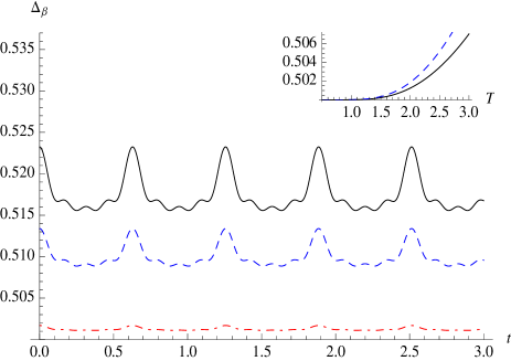
Figure 1: Time evolution of the thermal dependent uncertainty relation $\Delta_{\beta}(t)$ for three different values of the temperature $T=3.85\,(\beta=0.26)$ (full line), $T=3.57\,(\beta=0.28)$ (dashed line) and $T=1.96\,(\beta=0.51)$ (dotdashed line), from the upper to the lower curves, respectively . We take $g=1.0$, $\bar{\omega}=5.0$ and $\delta=0.1$; the scale for the temperature, the vertical axis and for time is in units such that $k_{B}=\hbar=c=1$; in the upper right small figure it is shown the temperature dependence of two neighboring minimum and maximum values of $\Delta_{\beta}(t)$, respectively full and dashed lines, for two times, $t\approx 2.3$ and $t\approx 2.5$, where they occur

Comments

Eq. (12) describes the time evolution of the uncertainty relation $\Delta q_{0}^{\prime}(t,\beta)\Delta p_{0}^{\prime}(t,\beta)\equiv\Delta(t,\beta)$ in a small cavity. A plot of this time evolution is given in Fig. 1 for some representative values of the temperature. The thermal uncertainty function, $\Delta(t,\beta)$, is an oscillating function which attains periodically an absolute minimum (maximum) value, ${\rm{Min}}[\Delta(t,\beta)]$ (${\rm{Max}}[\Delta(t,\beta)]$). Since the periodical character of $\Delta(t,\beta)$ does not involve $\beta$, the location of these extrema on the time axis do not depend on the temperature. Indeed, we can see from Fig.1, that the values of these minima and maxima depend on the temperature, $\beta^{-1}$, but appears to be, for each temperature, the same for all values of time where they occur, in other words the values of the absolute extrema appears to be independent of time. In the detail of Fig.1, are plotted two neighboring absolute minimum and maximum (corresponding to $t\approx 2.3$ and $t\approx 2.5$), as functions of temperature. We find from these figures that raising the temperature increases the amplitude of oscillation and the mean value of the uncertainty relation and that its lower and upper bounds, also grows with temperature.

We infer from Fig.1 that for a small cavity, in all cases an oscillatory behavior is present for $\Delta(t,\beta)$, with the amplitude of the oscillation depending on the temperature, $T$. For larger values of $T$ the amplitude of the oscillation, and both, its absolute minimum and maximum values, are larger than for lower temperatures. This behavior of the uncertainty principle is to be contrasted with the case of an arbitrarily large cavity (free space). In this last case, the product $(\Delta\,p)\,(\Delta\,q)$ goes, asymptotically, as $t\rightarrow\infty$ for each temperature, to a constant value $\Delta(\beta)$. This asymptotic value depends on the temperature and grows with it, but is independent of time. Distinctly, for a small cavity, even for $t\rightarrow\infty$, the product $(\Delta\,p)\,(\Delta\,q)$ presents oscillations, which have larger and larger amplitudes for higher temperatures.

The result above falls in a general context of the different behaviors of quantum systems confined in cavities, as compared to free space, in both, zero or finite temperature, the system being investigated using the formalism presented in this report. In adolfo3 some of us got the expected result that the probability, $P(t)$, that a simple cold atom in free space, excited at $t=0$ remain excited after an elapsed time $t$, decays monotonically, going to zero as $t\rightarrow\infty$, while in a small cavity, $P(t)$ has an oscillatory behavior, never reaching zero. For $\bar{\omega}\sim 10^{14}$ (in the visible red), $R\approx 10^{-6}{\rm{m}}$, in a weak (of the order of electromagnetic) coupling regime, ${\rm{Min}}\,P(t)\approx 0.98$, which is in agreement with experimental observations Haroche3 . At finite temperature it is obtained in termica , for a small cavity, that the occupation number of a simple atom in a heated environment has an oscillatory behavior with time and that its mean value increases with increasing temperature. In emaranho ; erico the behavior of an entangled bipartite system at zero and finite temperature is investigated; taking two measures of entanglement, it results an oscillatory behavior for a small cavity (entanglement is preserved at all times), while it disappears as $t\rightarrow\infty$ for free space.

We hope that the result presented in this report could have some usefulness in nanophysics or in quantum information theory. At this moment we are not able to comment about these aspects; they will be subject of future studies.

Acknowledgements: The author thanks FAPERJ and CNPq (brazilian agencies) for partial financial support.

References

- (1) W.G. Unruh, W.H. Zurek, Phys. Rev. D, 40, 1071 (1989)
- (2) B.L. Hu, Juan Pablo Paz, Yuhong Zhang, Phys, Rev. D, 45, 2843 (1992)
- (3) F. Haake, R. Reibold, Phys. Rev. A, 32, 2462 (1982)
- (4) A.O. Caldeira, A.J. Legget, Ann. Phys. (N.Y) 149, 374 (1983)
- (5) F. C. Khanna, A. P. C. Malbouisson, J. M. C. Malbouisson and A. E. Santana, Thermal Quantum Field Theory: Algebraic Aspects and Applications (World Scientific, Singapore, 2009).
- (6) G. Flores-Hidalgo, C. A. Linhares, A. P. C. Malbouisson and J. M. C. Malbouisson, J. Phys. A 41, 075404 (2008).
- (7) G. Flores-Hidalgo, A. P. C. Malbouisson, J. M. C. Malbouisson, Y. W. Milla and A. E. Santana, Phys. Rev. A 79, 032105 (2009).
- (8) F. C. Khanna, A. P. C. Malbouisson, J. M. C. Malbouisson and A.E. Santana, Phys. Rev. A 81, 032119 (2010).
- (9) E. R. Granhen, C. A. Linhares, A. P. C. Malbouisson and J. M. C. Malbouisson, Phys. Rev. A 81, 053820 (2010); C. A. Linhares, A. P. C. Malbouisson and J. M. C. Malbouisson, Phys. Rev. A 82, 055805 (2010).
- (10) E.G. Figueiredo, C. A. Linhares, A. P. C. Malbouisson and J. M. C. Malbouisson, Phys. Rev. A 84, 045802 (2011).
- (11) Aashish Clerk, Nature Nanotechnology 4, 796 (2009)
- (12) Sumiyoshi Abe and Norikazu Suzuki , Phys. Rev. A 41, 4608 (1990)
- (13) B. L. Hu, Yuhong Zhang , Mod. Phys. Lett. A8 3575 (1993)
- (14) B. L. Hu, Yuhong Zhang , Int.J.Mod.Phys. A10 4537 (1995)
- (15) G. Amelino-Camelia, M. Arzano, Yi Ling and G. Mandanici Class. and Quant Grav. 23, 2585 (2006)
- (16) N.P.Andion, A.P.C. Malbouisson and A. Mattos Neto, J.Phys.A34, 3735, (2001)
- (17) G. Flores-Hidalgo, A.P.C. Malbouisson, Phys. Rev. A66, 042118 (2002).
- (18) A.P.C. Malbouisson, Annals of Physics 308, 373 (2003).
- (19) G. Flores-Hidalgo and A.P.C. Malbouisson, Phys. Lett. A 337, 37 (2005).
- (20) W. Thirring, F. Schwabl, Ergeb. Exakt. Naturw. 36, 219 (1964)
- (21) C. Cohen-Tannoudji, Atoms in Electromagnetic Fields, (World Scientific, Singapure, 1994).
- (22) T. Petrosky, G. Ordonez and I. Prigogine, Phys. Rev. A 68, 022107 (2003).
- (23) Notice that our dressed states are not the same as those employed in studies involving the interaction of atoms and electromagnetic fields bouquinCohen and in the study of the radiation damping of classical systems petrosky .
- (24) W. Jhe, A. Anderson, E.A. Hinds, D. Meschede, L. Moi, S. Haroche, Phys. Rev. Lett., 58, 666 (1987)