Representability Conditions
by Grassmann Integration

Abstract

Representability conditions on the one- and two-particle density matrix for fermion systems are formulated by means of Grassmann integrals. A positivity condition for a certain kind of Grassmann integral is established which, in turn, induces the well-known G-, P- and Q-Conditions of quantum chemistry by an appropriate choice of the integrand. Similarly, the $\mathrm{T}_{1}$- and $\mathrm{T}_{2}$-Conditions are derived. Furthermore, quasifree Grassmann states are introduced and, for every operator $\widetilde{\gamma}\in\mathcal{H}\oplus\mathcal{H}$ with $0\leq\widetilde{\gamma}\leq\mathbbm{1}$, the existence of a unique quasifree Grassmann state whose one-particle density matrix is $\widetilde{\gamma}$ is shown.

1 Introduction

The grand canonical energy (minus pressure) $E_{0}\left(\mu\right):=\inf\left\{\sigma\left\{\widehat{\mathbbm{H}}-\mu\widehat{\mathbbm{N}}\right\}\right\}$ at sufficiently large chemical potential $\mu\geq 0$ of a quantum system with a Hamiltonian $\widehat{\mathbbm{H}}$ and particle number operator $\widehat{\mathbbm{N}}$ is given by the Rayleigh–Ritz principle as

$$E_{0}\left(\mu\right)=\inf\left\{\mathrm{Tr}\left\{\rho^{\frac{1}{2}}\big{(}\widehat{\mathbbm{H}}-\mu\widehat{\mathbbm{N}}\big{)}\rho^{\frac{1}{2}}\right\}\Big{|}\ \rho\in DM\right\},$$ (1)

where $\widehat{\mathbbm{H}}=\widehat{\mathbbm{H}}^{*}$ is a self-adjoint operator obeying stability of matter, i.e., bounded below by $-c\widehat{\mathbbm{N}}$ for some $c<\infty$, and being at most quartic in the creation and annihilation operators [11, 18]. This is typically the case for models of non-relativistic matter in physics and chemistry. The Pauli principle plays a crucial role for stability of matter to hold true, and we thus restrict our attention to fermion systems. On the fermion Fock space $\wedge\mathcal{H}$, the variation on the r.h.s. of (1) is over the set

$$DM:=\left\{\rho\,\Big{|}\ \rho\in\mathcal{L}_{+}^{1}\left(\wedge\mathcal{H}\right),\ \mathrm{Tr}\left\{\rho\right\}=1,\ \big{<}\widehat{\mathbbm{N}}^{2}\big{>}_{\rho}<\infty\right\},$$

i.e., density matrices with finite particle number variance. Here, the expectation value of an observable $\widehat{\mathbbm{A}}$ is

$$\big{<}\widehat{\mathbbm{A}}\big{>}_{\rho}:=\mathrm{Tr}\left\{\rho^{\frac{1}{2}}\widehat{\mathbbm{A}}\rho^{\frac{1}{2}}\right\}.$$

More specifically, if

$$\widehat{\mathbbm{H}}-\mu\widehat{\mathbbm{N}}=\sum\limits_{k,m}h_{km}{c}^{*}(f_{k}){c}(f_{m})+\sum\limits_{k,l,m,n}V_{klmn}{c}^{*}(f_{l}){c}^{*}(f_{k}){c}(f_{m}){c}(f_{n}),$$

then

$$E_{0}\left(\mu\right)=\inf\left\{\mathcal{E}\left(\gamma_{\rho},\Gamma_{\rho}\right)|\ \rho\in DM\right\},$$ (2)

where

$$\mathcal{E}\left(\gamma_{\rho},\Gamma_{\rho}\right)=\sum\limits_{k,m}h_{km}\left<f_{m},\gamma_{\rho}f_{k}\right>+\sum\limits_{k,l,m,n}V_{klmn}\left<f_{m}\otimes f_{n},\Gamma_{\rho}\left(f_{k}\otimes f_{l}\right)\right>$$

and the one- and two-particle density matrices corresponding to $\rho$ are defined by

$$\left<f,\gamma_{\rho}g\right> :=\left<{c}^{*}(g){c}(f)\right>_{\rho}\quad\text{and}$$

$$\left<f\otimes g,\Gamma_{\rho}\big{(}\tilde{f}\otimes\tilde{g}\big{)}\right> :=\left<{c}^{*}(\tilde{g}){c}^{*}\big{(}\tilde{f}\big{)}{c}(f){c}(g)\right>_{\rho},$$

respectively, for all $f,g,\tilde{f},\tilde{g}\in\mathcal{H}$. Note that (2) can be rewritten as

$$E_{0}\left(\mu\right)=\inf\left\{\mathcal{E}\left(\gamma,\Gamma\right)|\ \left(\gamma,\Gamma\right)\in\mathcal{R}\right\},$$ (3)

where

$$\mathcal{R}:=\left\{\left(\gamma,\Gamma\right)\in\mathcal{L}^{1}\left(\mathcal{H}\right)\times\mathcal{L}^{1}\left(\mathcal{H}\otimes\mathcal{H}\right)\Big{|}\ \exists\rho\in DM:\ \left(\gamma,\Gamma\right)=\left(\gamma_{\rho},\Gamma_{\rho}\right)\right\}$$

denotes the set of all representable one- and two-particle density matrices. Equation (3) suggests that the search for a minimizing $\rho$ could be drastically simplified if one would find a characterization of all representable reduced density matrices $\left(\gamma,\Gamma\right)$. This was realized almost fifty years ago [5, 7, 9, 12], but such a characterization is still unknown.

The characterization of $E_{0}\left(\mu\right)$ by (3) immediately yields lower bounds of the form

$$E_{0}\left(\mu\right)=:E_{\mathcal{R}}\left(\mu\right)\geq E_{\mathcal{S}}\left(\mu\right),$$ (4)

for any superset $\mathcal{S}$ of $\mathcal{R}$. For example, the positivity $\left<P_{2}^{*}P_{2}\right>_{\rho}\geq 0$ for all polynomials $P_{2}\equiv P_{2}\left({c}^{*},{c}\right)$ in the creation and annihilation operators of degree two yields the so-called G-, P-, and Q-Conditions on $\left(\gamma_{\rho},\Gamma_{\rho}\right)$ [2, 5, 7, 9]. Similarly, the positivity $\left<P_{3}^{*}P_{3}+P_{3}P_{3}^{*}\right>_{\rho}\geq 0$ yields the $\mathrm{T}_{1}$- and generalized $\mathrm{T}_{2}$-Conditions [7]. Hence, all representable reduced density matrices $\left(\gamma,\Gamma\right)$ necessarily fulfill the G-, P-, Q-, $\mathrm{T}_{1}$-, and generalized $\mathrm{T}_{2}$-Conditions, and we have

$$E_{\mathcal{R}}\left(\mu\right)\geq E_{\mathcal{S}\left[\mathrm{G,P,Q,}\mathrm{T}_{1},\mathrm{T}_{2}\right]}\left(\mu\right)\geq E_{\mathcal{S}\left[\mathrm{G,P,Q}\right]}\left(\mu\right),$$ (5)

since $\mathcal{R}\subseteq\mathcal{S}\left[\mathrm{G,P,Q,}\mathrm{T}_{1},\mathrm{T}_{2}\right]\subseteq\mathcal{S}\left[\mathrm{G,P,Q}\right]$, with

$$\mathcal{S}\left[X\right]:=\left\{\left(\gamma,\Gamma\right)\in\mathcal{L}^{1}\left(\mathcal{H}\right)\times\mathcal{L}^{1}\left(\mathcal{H}\otimes\mathcal{H}\right)\Big{|}\ \left(\gamma,\Gamma\right)\ \mathrm{fulfills}\ \mathrm{Conditions}\ X\right\}.$$

We have discussed (4)-(5) for $\mathcal{S}=\mathcal{S}\left[\mathrm{G,P}\right]$ in some detail in [2] and refer the reader to that paper and references therein. Furthermore, for $\mathcal{S}=\mathcal{S}\left[\mathrm{G,P,Q,}\mathrm{T}_{1},\mathrm{T}_{2}\right]$ numerical works show agreement with Full CI computations [4, 13, 14, 19] to high accuracy.

The purpose of the present paper is the reformulation of representability conditions in terms of Grassmann integrals. Such a transcription may possibly yield new viewpoints and hopefully new insights into the representability problem. To this end, we introduce a Grassmann algebra $\mathcal{G}_{M}$ as a finite dimensional complex algebra. The object on $\mathcal{G}_{M}$ corresponding to a given density matrix is an element of the form $\vartheta^{*}\star\vartheta$ described in the sequel. Grassmann integration is the basic and most commonly used method (see, e.g., [8, 16]) in theoretical physics to compute partition functions of the form

$$Z_{\Gamma,\lambda}\left(J\right):=\int\mathrm{D}_{\Gamma}(\phi)\,\mathrm{e}^{-S_{\Gamma}+\left(J,\phi\right)_{\Gamma}}$$

as a functional integral with $\mathrm{D}_{\Gamma}(\phi):=\prod\limits_{x\in\Gamma}\mathrm{d}\phi\left(x\right)$ with sources $J:\Gamma\to\mathbbm{R}$ and an action $S_{\Gamma}$ (see [16] for further details).

The derivation of the G-, P-, Q-, $\text{T}_{1}$-, and generalized $\text{T}_{2}$-Conditions is based on the representation of the trace on $\wedge\mathcal{H}$ in terms of Grassmann integrals and a positivity condition of a Grassmann integral, namely

$$\forall\eta\in\mathcal{G}_{M}:\ \int\mathrm{d}(\overline{\Psi},\Psi)\,\mathrm{e}^{2\left(\overline{\Psi},\Psi\right)}\eta^{*}\star\eta\geq 0,$$ (6)

where $\int\mathrm{d}(\overline{\Psi},\Psi)$ denotes the Grassmann integration. The star product refers to a product on $\mathcal{G}_{M}$ and is introduced later. Considering appropriate subspaces of $\mathcal{G}_{M}$ denoted by $\mathcal{G}_{M}^{(n)}$, the main results of this paper are the bounds for the one-particle density matrix $\gamma_{\vartheta}$:

$$\left\{\forall\mu\in\mathcal{G}_{M}^{(1)}:\int\mathrm{d}(\overline{\Psi},\Psi)\,\mathrm{e}^{2\left(\overline{\Psi},\Psi\right)}\vartheta^{*}\star\vartheta\star\mu\geq 0\right\}\Leftrightarrow\left\{0\leq\gamma_{\vartheta}\leq\mathbbm{1}\right\}$$

and the G-, P-, and Q-Condition as conditions for the two-particle density matrix $\Gamma_{\vartheta}$:

$$\left\{\forall\mu\in\mathcal{G}_{M}^{(2)}:\int\mathrm{d}(\overline{\Psi},\Psi)\,\mathrm{e}^{2\left(\overline{\Psi},\Psi\right)}\vartheta^{*}\star\vartheta\star\mu\geq 0\right\}\Leftrightarrow\left\{0\leq\gamma_{\vartheta}\leq\mathbbm{1},\ \text{G-, P-, and Q-Condition}\right\}$$

Finally, we prove the validity of the $\text{T}_{1}$- and generalized $\text{T}_{2}$-Condition by Inequality (6).

2 Reduced Density Matrices and Representability

Before we elucidate how to derive the G-, P-, Q-, $\mathrm{T}_{1}$-, and generalized $\mathrm{T}_{2}$-Conditions for the 1- and 2-particle density matrix (1- and 2-pdm) by Grassmann integration, we give a definition of these first two reduced density matrices. For this purpose, we consider a finite-dimensional index set $M$, an $|M|$-dimensional (one-particle) Hilbert space $\left(\mathcal{H},\ \left<\,\cdot\,,\,\cdot\,\right>\right)$, and an arbitrary, but fixed orthonormal basis (ONB) $\left\{\psi_{i}\right\}_{i\in M}$ of $\mathcal{H}$. Furthermore, we introduce the usual fermion creation and annihilation operators on the fermion Fock space $\wedge\mathcal{H}$ over $\mathcal{H}$ given by ${c}^{*}(\psi_{i})\equiv{c}^{*}_{i}$ and ${c}(\psi_{i})\equiv{c}_{i}$ with the canonical anticommutation relations (CAR)

$$\left\{{c}(f),{c}(g)\right\}=\left\{{c}^{*}(f),{c}^{*}(g)\right\}=0\ \ \text{and}\ \left\{{c}(f),{c}^{*}(g)\right\}=\left<f,g\right>\cdot\mathbbm{1}_{\wedge\mathcal{H}}$$ (7)

for all $f,g\in\mathcal{H}$, where $\left<\,\cdot\,,\,\cdot\,\right>$ is linear in the second and antilinear in the first argument. $\left\{A,B\right\}:=AB+BA$ denotes the anticommutator.

The 1-pdm $\gamma_{\rho}\in\mathcal{L}_{+}^{1}\left(\mathcal{H}\right)$ of a density matrix $\rho$, i.e., a positive trace class operator on $\wedge\mathcal{H}$ of unit trace ($\mathrm{tr}_{\wedge\mathcal{H}}\left\{\rho\right\}=1$), is defined by its matrix elements as

$$\forall f,g\in\mathcal{H}:\ \left<f,\gamma_{\rho}g\right> :=\text{tr}_{\wedge\mathcal{H}}\left\{\rho\,{c}^{*}(g){c}(f)\right\}.$$ (8)

Likewise, the 2-pdm $\Gamma_{\rho}\in\mathcal{L}_{+}^{1}\left(\mathcal{H}\otimes\mathcal{H}\right)$ of $\rho$ is defined by

$$\forall f_{1},f_{2},g_{1},g_{2}\in\mathcal{H}:\ \left<f_{1}\otimes f_{2},\Gamma_{\rho}(g_{1}\otimes g_{2})\right>:=\text{tr}_{\wedge\mathcal{H}}\left\{\rho\,{c}^{*}(g_{2}){c}^{*}(g_{1}){c}(f_{1}){c}(f_{2})\right\}.$$ (9)

There are several properties which can be derived directly from the definition of $\gamma_{\rho}$ and $\Gamma_{\rho}$.

Lemma 2.1.

Let $\rho\in\mathcal{L}_{+}^{1}(\wedge\mathcal{H})$ be a density matrix and $\widehat{\mathbbm{N}}:=\sum\limits_{k\in M}{c}^{*}_{k}{c}_{k}$ the particle number operator with $\big{<}\widehat{\mathbbm{N}}^{2}\big{>}_{\rho}<\infty$. Then the following assertions hold true:

• $\gamma_{\rho}\in\mathcal{L}_{+}^{1}(\mathcal{H})$, $0\leq\gamma_{\rho}\leq\mathbbm{1}$, $\mathrm{tr}_{\mathcal{H}}\left\{\gamma_{\rho}\right\}=\big{<}\widehat{\mathbbm{N}}\big{>}_{\rho}$, $\Gamma_{\rho}\in\mathcal{L}_{+}^{1}(\mathcal{H}\otimes\mathcal{H})$, $0\leq\Gamma_{\rho}\leq\big{<}\widehat{\mathbbm{N}}\big{>}_{\rho}$, and $\mathrm{tr}_{\mathcal{H}\otimes\mathcal{H}}\left\{\Gamma_{\rho}\right\}=\big{<}\widehat{\mathbbm{N}}\big{(}\widehat{\mathbbm{N}}-\mathbbm{1}\big{)}\big{>}_{\rho}$.

• If $\mathrm{Ran}\left\{\rho\right\}\subseteq\wedge^{(N)}\mathcal{H}$, $N\in\mathbbm{N}$, then, for all $f,g\in\mathcal{H}$,

  $$\left<f,\gamma_{\rho}g\right>=\frac{1}{N-1}\sum\limits_{k\in M}\left<f\otimes\varphi_{k},\Gamma_{\rho}(g\otimes\varphi_{k})\right>,$$

  where $\left\{\varphi_{k}\right\}_{k\in M}\subseteq\mathcal{H}$ is an ONB. Here, $\wedge^{(N)}\mathcal{H}$ denotes the fermion $N$-particle Fock space.

• Furthermore,

  $$\rho=\left|{c}^{*}(\varphi_{1})\cdots{c}^{*}(\varphi_{N})\Omega\right>\left<{c}^{*}(\varphi_{1})\cdots{c}^{*}(\varphi_{N})\Omega\right|\ \ \Leftrightarrow\ \ \gamma_{\rho}=\sum\limits_{i=1}^{N}\left|\varphi_{i}\right>\left<\varphi_{i}\right|$$

  and, in this case,

  $$\Gamma_{\rho}=\left(\mathbbm{1}-\mathrm{Ex}\right)\left(\gamma_{\rho}\otimes\gamma_{\rho}\right),$$

  where $\mathrm{Ex}\left(f\otimes g\right):=g\otimes f$ for any $f,g\in\mathcal{H}$.

For further details we recommend [1, 2, 5, 9]. A proof can be found in [1]. Beside these properties, necessary conditions on $\left(\gamma,\Gamma\right)$ to be representable were derived in [5, 7, 9]. In particular, the P-, G-, and Q-Conditions are:

• $\left\{\left(\gamma,\Gamma\right)\ \mathrm{fulfills}\ \text{P-Condition}\right\}:\Leftrightarrow\left\{\Gamma\geq 0\right\},$

• $\left\{\left(\gamma,\Gamma\right)\ \mathrm{fulfills}\ \text{G-Condition}\right\}\\ \qquad:\Leftrightarrow\left\{\forall A\in\mathcal{B}\left(\mathcal{H}\right):\ \mathrm{tr}\left\{\left(A^{*}\otimes A\right)\left(\Gamma+\mathrm{Ex}\left(\gamma\otimes\mathbbm{1}\right)\right)\right\}\geq\left|\mathrm{tr}\left\{A\gamma\right\}\right|^{2}\right\},$

• $\left\{\left(\gamma,\Gamma\right)\ \mathrm{fulfills}\ \text{Q-Condition}\right\}\\ :\Leftrightarrow\left\{\Gamma+\left(\mathbbm{1}-\mathrm{Ex}\right)\left(\mathbbm{1}\otimes\mathbbm{1}-\gamma\otimes\mathbbm{1}-\mathbbm{1}\otimes\gamma\right)\geq 0\right\}.$

The $\mathrm{T}_{1}$- and generalized $\mathrm{T}_{2}$-Conditions are more complicated and not given here. For this conditions we refer the reader to [7] or Subsection 5.3 of this work.

3 Grassmann Algebras

We introduce the Grassmann algebra as the complex algebra generated by elements of the set $\left\{\overline{\psi}_{i},\psi_{i}\right\}_{i\in M}$ with $|M|<\infty$ modulo the anticommutation relations specified below. A product of two generators is denoted by $\psi_{i}\cdot\psi_{j}\equiv\psi_{i}\psi_{j}$. The unity is given as $1\cdot\psi_{i}=\psi_{i}\cdot 1=\psi_{i}$ (and equivalently for $\overline{\psi}_{j}$). The anticommutation relations allow us to find a one-to-one representation of the CAR of fermion creation and annihilation operators in terms of Grassmann variables. For further details on this well-known material we recommend [6, 15, 16, 17]. We use the notation of [15].

Definition 3.1.

For an ordered set $I:=\left\{i_{1},\dots,i_{m}\right\}\subseteq M$ we write

$$\Psi_{I}:=\psi_{i_{1}}\cdots\psi_{i_{m}},\quad\overline{\Psi}_{I}:=\overline{\psi}_{i_{1}}\cdots\overline{\psi}_{i_{m}}.$$

For $I=\emptyset$ we set $\Psi_{I}=\overline{\Psi}_{I}=1$. Denoting the reversely ordered set corresponding to $I$ by $I^{\prime}$, we write

$$\Psi_{I^{\prime}}:=\psi_{i_{m}}\cdots\psi_{i_{1}}.$$

Definition 3.2.

Given a set of generators $\left\{\overline{\psi}_{i},\psi_{i}\right\}_{i\in M}$ obeying the anticommutation relations

$$\overline{\psi}_{i}\psi_{j}+\psi_{j}\overline{\psi}_{i}=\overline{\psi}_{i}\overline{\psi}_{j}+\overline{\psi}_{j}\overline{\psi}_{i}=\psi_{i}\psi_{j}+\psi_{j}\psi_{i}=0\quad\forall\,i,j\in M,$$

the Grassmann algebra $\mathcal{G}_{M}$ is defined as

$$\mathcal{G}_{M}:=\mathrm{span}\left\{\overline{\Psi}_{I}\Psi_{J}|\ I,J\subseteq M\right\}.$$

Introducing the ordinary wedge product, we can identify $\mathcal{G}_{M}$ with the Fock space $\wedge\left(\overline{\mathcal{H}}\oplus\mathcal{H}\right)$ of a Hilbert space $\left(\mathcal{H},\ \left<\,\cdot\,,\,\cdot\,\right>\right)$ with finite dimension $|M|$. Considering $\mathcal{H}$ as a subset of $\mathcal{G}_{M}$, we can identify $\left\{\psi_{i}\right\}_{i\in M}$ with a fixed ONB of $\mathcal{H}$ and $\left\{\overline{\psi}_{i}\right\}_{i\in M}$ with the corresponding ONB of $\overline{\mathcal{H}}$, i.e., the space of all continuous linear functionals $\mathcal{H}\rightarrow\mathbbm{C},\ \psi_{i}\mapsto\overline{\psi}_{i}\left(\,\cdot\,\right):=\left<\psi_{i},\cdot\,\right>$.

Remark 3.3.

If $\mathcal{G}_{M}$ is generated by $\left\{\overline{\phi}_{i},\phi_{i}\right\}_{i\in M}$, we emphasize this by using $\mu\left(\overline{\phi},\phi\right)\in\mathcal{G}_{M}$ instead of $\mu\in\mathcal{G}_{M}$. We also use “mixed” generators, e.g.,

$$\mu\left(\overline{\psi},\phi\right):=\sum\limits_{i,j}\alpha_{ij}\,\overline{\Psi}_{I_{i}}\Phi_{J_{j}}.$$

Later, it is necessary to link the CAR algebra of fermion annihilation and creation operators to a Grassmann algebra. For this purpose, a map between $\mathcal{B}\left(\wedge\mathcal{H}\right)$ and $\mathcal{G}_{M}$ as an isomorphism between vector spaces is required. This map is provided below.

Definition 3.4.

Let $\mathcal{G}_{M}$ be generated by $\left\{\overline{\psi}_{i},\psi_{i}\right\}_{i\in M}$ and associate $\left\{\psi_{i}\right\}_{i\in M}$ with a fixed ONB of $\mathcal{H}$. For all $z\in\mathbbm{C}$ and $m,n\leq|M|$, we define the linear map $\Theta:\mathcal{B}\left(\wedge\mathcal{H}\right)\to\mathcal{G}_{M}$ by $\Theta\left(z\right):=z$ and

$$\Theta\left({c}^{*}(\psi_{i_{1}})\cdots{c}^{*}(\psi_{i_{m}}){c}(\psi_{j_{1}})\cdots{c}(\psi_{j_{n}})\right):=\overline{\psi}_{i_{1}}\cdots\overline{\psi}_{i_{m}}\psi_{j_{1}}\cdots\psi_{j_{n}},$$ (10)

and extension to $\mathcal{B}\left(\wedge\mathcal{H}\right)$ by linearity.

We emphasize that $\Theta$ is not multiplicative. E.g., while

$$\Theta\big{(}{c}^{*}(\psi_{1}){c}(\psi_{1})\big{)}=\overline{\psi}_{1}\psi_{1}=\Theta\big{(}{c}^{*}(\psi_{1})\big{)}\Theta\big{(}{c}(\psi_{1})\big{)},$$

we have

$$\Theta\big{(}{c}(\psi_{1}){c}^{*}(\psi_{1})\big{)} =\Theta\big{(}-{c}^{*}(\psi_{1}){c}(\psi_{1})+\mathbbm{1}\big{)}$$

$$=-\overline{\psi}_{1}\psi_{1}+1=\psi_{1}\overline{\psi}_{1}+1=\Theta\big{(}{c}(\psi_{1})\big{)}\Theta\big{(}{c}^{*}(\psi_{1})\big{)}+1.$$

Thus, Equation (10) only holds for normal-ordered monomials in creation and annihilation operators, i.e., monomials in which all creation operators are to the left of all annihilation operators.

Definition 3.5.

For any $A\in\mathcal{B}\left(\mathcal{H}\right)$ we set

$$\left(\overline{\Psi},A\Phi\right):=\sum\limits_{i,j\in M}\left[\overline{\psi}_{i}\left(A\psi_{j}\right)\right]\overline{\psi}_{j}\phi_{i}\in\mathcal{G}_{M}.$$

Note that $\overline{\psi}_{i}\left(A\psi_{j}\right)=\left<\psi_{i},A\psi_{j}\right>\in\mathbbm{C}$. Furthermore, $\left(\overline{\Psi},A\Phi\right)$ does not depend on the choice of generators of $\mathcal{G}_{M}$ as can be seen by a unitary change of generators, e.g., $\chi_{i}:=\sum\limits_{j\in M}U_{ij}\psi_{j}$ for unitary $U$. An important case is $A=\mathrm{id}_{\mathcal{H}}$. Here we have $\left(\overline{\Psi},\Phi\right)=\sum\limits_{i\in M}\overline{\psi}_{i}\phi_{i}$. One of the last ingredients for the Grassmann integration is the following.

Definition 3.6.

The expression $\mathrm{e}^{\pm\left(\overline{\Psi},A\Phi\right)}\in\mathcal{G}_{M}$ is given by

$$\mathrm{e}^{\pm\left(\overline{\Psi},A\Phi\right)}:=\sum\limits_{m=0}^{\infty}\frac{1}{m!}\left[\pm\left(\overline{\Psi},A\Phi\right)\right]^{m}.$$

As $\mathrm{dim}\left\{\wedge\mathcal{H}\right\}=2^{\mathrm{dim}\left\{\mathcal{H}\right\}}$, the sum runs only over $0\leq m\leq 2^{\mathrm{dim}\left\{\mathcal{H}\right\}}$.

Remark 3.7.

Since $\left(\overline{\Psi},\Phi\right)=\sum\limits_{\alpha\in M}\overline{\psi}_{\alpha}\phi_{\alpha}$, and $\overline{\psi}_{\alpha}\phi_{\alpha}$ commutes with every element of $\mathcal{G}_{M}$, we have

$$\mathrm{e}^{\pm\left(\overline{\Psi},\Phi\right)}=\prod\limits_{\alpha\in M}\left(1\pm\overline{\psi}_{\alpha}\phi_{\alpha}\right).$$ (11)

Definition 3.8.

For all $i,j\in M$, we define the vector space homomorphisms $\frac{\delta}{\delta\psi_{i}},\ \frac{\delta}{\delta\overline{\psi}_{i}}:\mathcal{G}_{M}\to\mathcal{G}_{M}$ by

$$\frac{\delta}{\delta\psi_{i}}\psi_{j}=\frac{\delta}{\delta\overline{\psi}_{i}}\overline{\psi}_{j}=\delta_{ij},\quad\mathrm{and}\quad\frac{\delta}{\delta\psi_{i}}\overline{\psi}_{j}=\frac{\delta}{\delta\overline{\psi}_{i}}\psi_{j}=0.$$

Remark 3.9.

The set $\left\{\frac{\delta}{\delta\overline{\psi}_{i}},\frac{\delta}{\delta\psi_{i}}\right\}_{i\in M}$ itself generates a Grassmann algebra.

4 Grassmann Integration

Now we are prepared to define the Grassmann integral, which is a linear operator from $\mathcal{G}_{M}$ to $\mathbbm{C}$.

Definition 4.1.

The map $\int\mathrm{d}(\overline{\Psi},\Psi):\ \mathcal{G}_{M}\to\mathbbm{C}$ is defined by

$$\int\mathrm{d}(\overline{\Psi},\Psi):=\prod\limits_{\alpha\in M}\left(\frac{\delta}{\delta\overline{\psi}_{\alpha}}\frac{\delta}{\delta\psi_{\alpha}}\right).$$

and is referred to as the Grassmann integral.

Remark 4.2.

If the factor $\mathrm{e}^{2\left(\overline{\Psi},\Psi\right)}=\prod\limits_{\alpha\in M}\left(1+2\overline{\psi}_{\alpha}\psi_{\alpha}\right)$ is involved in the integration, we use the abbreviation

$$\mathcal{D}(\overline{\Psi},\Psi):=\mathrm{d}(\overline{\Psi},\Psi)\,\mathrm{e}^{2\left(\overline{\Psi},\Psi\right)},$$

since $\prod\limits_{\alpha\in M}\left(1+2\overline{\psi}_{\alpha}\psi_{\alpha}\right)$ commutes with every element of $\mathcal{G}_{M}$.

In order to state the invariance of the Grassmann integration with respect to a change of generators, we introduce some notations. We write two sets of generators, $\left\{\overline{\psi}_{i},\psi_{i}\right\}_{i\in M}$ and $\left\{\overline{\chi}_{i},\chi_{i}\right\}_{i\in M}$, as $2|M|$-component vectors $\underline{a}$ and $\underline{b}$, respectively, whose entries are given by

$$a_{i}:=\overline{\psi}_{i}\ \text{and}\ a_{|M|+i}:=\psi_{i},\quad\text{and}\quad b_{i}:=\overline{\chi}_{i}\ \text{and}\ b_{|M|+i}:=\chi_{i}.$$ (12)

where for all $i\in M$. Furthermore, we define the entries of the $2|M|$-component vectors $\frac{\delta}{\delta\underline{a}}$ and $\frac{\delta}{\delta\underline{b}}$ by

$$\frac{\delta}{\delta\underline{a}_{i}}:=\frac{\delta}{\delta\overline{\psi}_{i}}\ \text{and}\ \frac{\delta}{\delta\underline{a}_{|M|+i}}:=\frac{\delta}{\delta\psi_{i}},\quad\text{and}\quad\frac{\delta}{\delta\underline{b}_{i}}:=\frac{\delta}{\delta\overline{\chi}_{i}}\ \text{and}\ \frac{\delta}{\delta\underline{b}_{|M|+i}}:=\frac{\delta}{\delta\chi_{i}}.$$

We denote the index set for the introduced vectors by $\widetilde{M}$, $|\widetilde{M}|=2|M|$. In this notation the Grassmann integration with respect to $\left\{\overline{\psi}_{i},\psi_{i}\right\}_{i\in M}$ reads as

$$\left(-1\right)^{\frac{1}{2}|M|(|M|-1)}\prod\limits_{\alpha\in M}\left(\frac{\delta}{\delta\overline{\psi}_{\alpha}}\frac{\delta}{\delta\psi_{\alpha}}\right)=\prod\limits_{\alpha\in M}\frac{\delta}{\delta\overline{\psi}_{\alpha}}\prod\limits_{\alpha\in M}\frac{\delta}{\delta\psi_{\alpha}}=\prod\limits_{\beta\in\widetilde{M}}\frac{\delta}{\delta\underline{a}_{\beta}}.$$

Lemma 4.3.

The Grassmann integral does not depend on the choice of the generators. I.e., for $\underline{a}$ and $\underline{b}$ as defined in (12), and a transformation defined by

$$\underline{b}=U\,\underline{a},$$

where $U$ is a unitary $2|M|\times 2|M|$-matrix, we have

$$\frac{\delta}{\delta\underline{b}}=\overline{U}\frac{\delta}{\delta\underline{a}}$$

and, for any $\mu\in\mathcal{G}_{M}$,

$$\prod\limits_{\alpha\in M}\left(\frac{\delta}{\delta\overline{\psi}_{\alpha}}\frac{\delta}{\delta\psi_{\alpha}}\right)\mu\left(\overline{\psi},\psi\right)=\prod\limits_{\alpha\in M}\left(\frac{\delta}{\delta\overline{\chi}_{\alpha}}\frac{\delta}{\delta\chi_{\alpha}}\right)\mu\left(\overline{\chi},\chi\right).$$

Proof.

First we prove $\frac{\delta}{\delta\underline{b}}=\overline{U}\frac{\delta}{\delta\underline{a}}$. The identity $\frac{\delta}{\delta a_{j}}a_{i}=\delta_{ij}$ follows from the properties of the generators. An equivalent identity has to be claimed for $\frac{\delta}{\delta\underline{b}}\underline{b}$. Suppose $\frac{\delta}{\delta\underline{b}}$ transforms as $\frac{\delta}{\delta\underline{b}}=V\frac{\delta}{\delta\underline{a}}$ with a $2|M|\times 2|M|$-matrix $V$. This yields

$$\frac{\delta}{\delta b_{j}}b_{i} =\Bigg{(}\sum\limits_{\alpha\in\widetilde{M}}V_{j\alpha}\frac{\delta}{\delta a_{\alpha}}\Bigg{)}\Bigg{(}\sum\limits_{\beta\in\widetilde{M}}U_{i\beta}a_{\beta}\Bigg{)}=\left(UV^{T}\right)_{ij}.$$

In other words, we have $UV^{T}=\mathbbm{1}_{\widetilde{M}}$ and, thus, $V=\overline{U}$. Finally, we can prove the invariance of the Grassmann integral. For a given set of generators $\left\{\overline{\psi}_{i},\psi_{i}\right\}_{i\in M}$, any $\mu\in\mathcal{G}_{M}$ can be written as

$$\mu\equiv\mu\left(\overline{\psi},\psi\right)=\sum\limits_{I,J\subseteq M}\alpha_{IJ}\overline{\Psi}_{I}\Psi_{J},$$

where $\alpha_{IJ}\in\mathbbm{C}$ for all $I,J\subseteq M$, and $I,J$ ordered. The Grassmann integral of $\mu$ is

$$\int\mathrm{d}(\overline{\Psi},\Psi)\,\mu\left(\overline{\psi},\psi\right)=\int\mathrm{d}(\overline{\Psi},\Psi)\sum\limits_{I,J\subseteq M}a_{IJ}\overline{\Psi}_{I}\Psi_{J}=\int\mathrm{d}(\overline{\Psi},\Psi)\,\alpha_{MM}\overline{\Psi}_{M}\Psi_{M},$$

since all other terms of $\mu$ do not contribute to the integral. If the decomposition of $\mu$ yields $\alpha_{MM}=0$, the Grassmann integral of $\mu$ vanishes. In this case there is nothing to show. For $\alpha_{MM}\neq 0$ we consider the transformation of $\int\mathrm{d}(\overline{\Psi},\Psi)$ and $\overline{\Psi}_{M}\Psi_{M}$ separately. For $\int\mathrm{d}(\overline{\Psi},\Psi)$ we use $\frac{\delta}{\delta\underline{a}_{i}}\frac{\delta}{\delta\underline{a}_{j}}=-\frac{\delta}{\delta\underline{a}_{j}}\frac{\delta}{\delta\underline{a}_{i}}$ for $i\neq j$, and express $\frac{\delta}{\delta\underline{b}}$ in terms of $\frac{\delta}{\delta\underline{a}}$:

$$\left(\prod\limits_{\alpha\in M}\frac{\delta}{\delta\overline{\chi}_{\alpha}}\right)\left(\prod\limits_{\alpha\in M}\frac{\delta}{\delta\chi_{\alpha}}\right) =\prod\limits_{\beta\in\widetilde{M}}\frac{\delta}{\delta\underline{b}_{\beta}}=\sum\limits_{\beta_{1},\dots,\beta_{|\widetilde{M}|}\in\widetilde{M}}\prod\limits_{j\in\widetilde{M}}\overline{U}_{j\beta_{j}}\frac{\delta}{\delta\underline{a}_{\beta_{j}}}$$

$$=\sum\limits_{\pi\in\mathcal{S}_{\widetilde{M}}}\prod\limits_{j\in\widetilde{M}}\overline{U}_{j\pi(j)}\frac{\delta}{\delta\underline{a}_{\pi(j)}}=\sum\limits_{\pi\in\mathcal{S}_{\widetilde{M}}}\left(-1\right)^{\pi}\prod\limits_{j\in\widetilde{M}}\overline{U}_{j\pi(j)}\frac{\delta}{\delta\underline{a}_{j}}$$

$$=\mathrm{det}\left(\overline{U}\right)\prod\limits_{j\in\widetilde{M}}\frac{\delta}{\delta\underline{a}_{j}}.$$

Analogously, we have

$$\prod\limits_{\alpha\in M}\overline{\chi}_{M}\prod\limits_{\alpha\in M}\chi_{M}=\prod\limits_{\beta\in\widetilde{M}}b_{\beta}=\mathrm{det}\left(U\right)\prod\limits_{j\in\widetilde{M}}a_{j}.$$

Merging the results we obtain

$$\left(\prod\limits_{\alpha\in M}\frac{\delta}{\delta\overline{\chi}_{\alpha}}\right)\left(\prod\limits_{\alpha\in M}\frac{\delta}{\delta\chi_{\alpha}}\right)\prod\limits_{\alpha\in M}\overline{\chi}_{M}\prod\limits_{\alpha\in M}\chi_{M}=\left|\mathrm{det}\left(U\right)\right|^{2}\prod\limits_{j\in\widetilde{M}}\frac{\delta}{\delta\underline{a}_{j}}\prod\limits_{j\in\widetilde{M}}a_{j}.$$

The proof is complete with $\left|\mathrm{det}\left(U\right)\right|^{2}=1$, since $U$ is unitary. ∎

Remark 4.4.

The transformation $U$ mixes $\overline{\psi}_{i}$’s and $\psi_{i}$’s. For $U:=\begin{pmatrix}u&v\\ \overline{v}&\overline{u}\end{pmatrix}$, a transformation without mixing is given for $v=0$. In this case, $u$ has to be unitary.

For the application of the Grassmann integration on representability conditions we still need some tools, especially the definition of a product on $\mathcal{G}_{M}$ which induces the CAR on the Grassmann algebra.

Definition 4.5.

For all $\mu\equiv\mu\left(\overline{\psi},\psi\right)$ and $\eta\equiv\eta\left(\overline{\psi},\psi\right)\in\mathcal{G}_{M}$, we define the star product $\mu\star\eta\in\mathcal{G}_{M}$ by

$$\left(\mu\star\eta\right)\left(\overline{\psi},\psi\right):=\int\mathrm{d}(\overline{\Phi},\Phi)\,\mu\left(\overline{\psi},\phi\right)\eta\left(\overline{\phi},\psi\right)\mathrm{e}^{-\left(\overline{\Psi},\Psi\right)}\mathrm{e}^{\left(\overline{\Psi},\Phi\right)}\mathrm{e}^{-\left(\overline{\Phi},\Phi\right)}\mathrm{e}^{\left(\overline{\Phi},\Psi\right)}.$$

We calculate the star product of two monomials $\mu:=\overline{\Psi}_{I}\Psi_{J}$ and $\eta:=\overline{\Psi}_{K}\Psi_{L}$, which determines the star product in general, due to the linearity of the Grassmann integral.

Lemma 4.6.

Let $I,J,K,L\subseteq M$. Then we have

$$\left(\overline{\Psi}_{I}\Psi_{J}\right)\star\left(\overline{\Psi}_{K}\Psi_{L}\right)$$

$$\qquad\qquad=\sigma_{S}\sigma_{JS}\cdot\mathrm{e}^{-\left(\overline{\Psi},\Psi\right)}\overline{\Psi}_{I}\Psi_{J\backslash S}\overline{\Psi}_{K\backslash S}\Psi_{L}\prod\limits_{\begin{subarray}{c}\alpha\in M\\ \backslash\left(J\cup K\right)\end{subarray}}\left(1+\overline{\psi}_{\alpha}\psi_{\alpha}\right),$$ (13)

where $S:=J\cap K$ and $\sigma_{JS}:=\left(-1\right)^{|S|\left(|J\backslash S|+\frac{|S|-1}{2}\right)}$. The sign $\sigma_{S}$ is given by the identity $\sigma_{S}\Phi_{S}\Phi_{J\backslash S}\overline{\Phi}_{S}\overline{\Phi}_{K\backslash S}=\Phi_{J}\overline{\Phi}_{K}$.

Proof.

Writing $S:=J\cap K$, we face the integral

$$\left(\overline{\Psi}_{I}\Psi_{J}\right)\star\left(\overline{\Psi}_{K}\Psi_{L}\right) =\sigma_{S}\cdot\mathrm{e}^{-\left(\overline{\Psi},\Psi\right)}\overline{\Psi}_{I}\int\mathrm{d}(\overline{\Phi},\Phi)\,\Phi_{S}\Phi_{J\backslash S}\overline{\Phi}_{S}\overline{\Phi}_{K\backslash S}$$

$$\qquad\times\prod\limits_{\alpha\in M}\left(1+\overline{\phi}_{\alpha}\psi_{\alpha}+\overline{\psi}_{\alpha}\phi_{\alpha}-\overline{\phi}_{\alpha}\phi_{\alpha}-\overline{\phi}_{\alpha}\phi_{\alpha}\overline{\psi}_{\alpha}\psi_{\alpha}\right)\Psi_{L},$$

where we use

$$\prod\limits_{\alpha\in M}\left(1+\overline{\phi}_{\alpha}\psi_{\alpha}+\overline{\psi}_{\alpha}\phi_{\alpha}-\overline{\phi}_{\alpha}\phi_{\alpha}-\overline{\phi}_{\alpha}\phi_{\alpha}\overline{\psi}_{\alpha}\psi_{\alpha}\right)=\mathrm{e}^{\left(\overline{\Psi},\Phi\right)}\mathrm{e}^{-\left(\overline{\Phi},\Phi\right)}\mathrm{e}^{\left(\overline{\Phi},\Psi\right)}$$

as a consequence of (11). In the next step we write $M=\left(M\backslash\left(J\cup K\right)\right)\dot{\cup}\left(J\backslash S\right)\dot{\cup}\left(K\backslash S\right)\dot{\cup}S$ (where $\dot{\cup}$ denotes a disjoint union) and arrive at

$$\left(\overline{\Psi}_{I}\Psi_{J}\right)\star\left(\overline{\Psi}_{K}\Psi_{L}\right)= \sigma_{S}\sigma_{SJ}\cdot\mathrm{e}^{-\left(\overline{\Psi},\Psi\right)}\overline{\Psi}_{I}\int\mathrm{d}(\overline{\Phi},\Phi)\,\prod\limits_{\alpha\in S}\phi_{\alpha}\overline{\phi}_{\alpha}$$

$$\qquad\times\prod\limits_{\alpha\in J\backslash S}\left(\phi_{\alpha}+\phi_{\alpha}\overline{\phi}_{\alpha}\psi_{\alpha}\right)\prod\limits_{\alpha\in K\backslash S}\left(\overline{\phi}_{\alpha}+\overline{\phi}_{\alpha}\overline{\psi}_{\alpha}\phi_{\alpha}\right)$$

$$\qquad\times\prod\limits_{\begin{subarray}{c}\alpha\in M\\ \backslash\left(J\cup K\right)\end{subarray}}\left(1+\overline{\phi}_{\alpha}\psi_{\alpha}+\overline{\psi}_{\alpha}\phi_{\alpha}-\overline{\phi}_{\alpha}\phi_{\alpha}-\overline{\phi}_{\alpha}\phi_{\alpha}\overline{\psi}_{\alpha}\psi_{\alpha}\right)\Psi_{L}.$$

The sign $\sigma_{JS}:=\left(-1\right)^{|S|\left(|J\backslash S|+\frac{|S|-1}{2}\right)}$ occurs due to the permutation of all $\phi$’s in $\Phi_{S}$ with all $\phi$’s in $\Phi_{J\backslash S}$, and $\Phi_{S}\overline{\Phi}_{S}=\left(-1\right)^{\frac{1}{2}|S|\left(|S|-1\right)}\left(\prod\limits_{\alpha\in S}\phi_{\alpha}\overline{\phi}_{\alpha}\right)$. Now we can perform the integration and arrive at

$$\left(\overline{\Psi}_{I}\Psi_{J}\right)\star\left(\overline{\Psi}_{K}\Psi_{L}\right)=\sigma_{S}\sigma_{JS}\cdot\mathrm{e}^{-\left(\overline{\Psi},\Psi\right)}\overline{\Psi}_{I}\prod\limits_{\alpha\in J\backslash S}\psi_{\alpha}\prod\limits_{\alpha\in K\backslash S}\overline{\psi}_{\alpha}\prod\limits_{\begin{subarray}{c}\alpha\in M\\ \backslash\left(J\cup K\right)\end{subarray}}\left(1+\overline{\psi}_{\alpha}\psi_{\alpha}\right)\Psi_{L},$$

as claimed in (13), since all involved sets are disjoint. ∎

There are several properties of the star product which follow from Lemma 4.6.

Lemma 4.7.

For all $\mu,\eta,\nu\in\mathcal{G}_{M}$ we have

$$\mu\star\left(\eta\star\nu\right)=\left(\mu\star\eta\right)\star\nu.$$

Proof.

By the definition of the star product we have

$$\mu\star\left(\eta\star\nu\right) =\mu\left(\overline{\psi},\psi\right)\star\int\mathrm{d}(\overline{\Phi},\Phi)\,\eta\left(\overline{\psi},\phi\right)\nu\left(\overline{\phi},\psi\right)\mathrm{e}^{-\left(\overline{\Psi},\Psi\right)+\left(\overline{\Psi},\Phi\right)-\left(\overline{\Phi},\Phi\right)+\left(\overline{\Phi},\Psi\right)}$$

$$=\int\mathrm{d}(\overline{\Omega},\Omega)\int\mathrm{d}(\overline{\Phi},\Phi)\,\mu\left(\overline{\psi},\omega\right)\eta\left(\overline{\omega},\phi\right)\nu\left(\overline{\phi},\psi\right)$$

$$\qquad\qquad\times\mathrm{e}^{-\left(\overline{\Psi},\Psi\right)+\left(\overline{\Psi},\Omega\right)-\left(\overline{\Omega},\Omega\right)+\left(\overline{\Omega},\Phi\right)-\left(\overline{\Phi},\Phi\right)+\left(\overline{\Phi},\Psi\right)}.$$

Performing the integration with respect to $\left(\overline{\phi},\phi\right)$ we gain

$$\mu\star\left(\eta\star\nu\right)=\int\mathrm{d}(\overline{\Omega},\Omega)\,\mu\left(\overline{\psi},\omega\right)\eta\left(\overline{\omega},\psi\right)\mathrm{e}^{-\left(\overline{\Psi},\Psi\right)+\left(\overline{\Psi},\Omega\right)-\left(\overline{\Omega},\Omega\right)+\left(\overline{\Omega},\Psi\right)}\star\nu\left(\overline{\psi},\psi\right),$$

which is, in fact, $\left(\mu\star\eta\right)\star\nu$. ∎

According to the creation and annihilation operators on $\mathcal{B}\left(\wedge\mathcal{H}\right)$, there is also an implementation of the CAR for the generators of $\mathcal{G}_{M}$.

Lemma 4.8.

Let $\left\{\overline{\psi}_{i},\psi_{i}\right\}_{i\in M}$ be the generators of $\mathcal{G}_{M}$. For $\left\{\mu,\eta\right\}_{\star}:=\mu\star\eta+\eta\star\mu$ we have

$$\left\{\psi_{i},\psi_{j}\right\}_{\star}=\left\{\overline{\psi}_{i},\overline{\psi}_{j}\right\}_{\star}=0,\qquad\mathrm{and}\qquad\left\{\overline{\psi}_{i},\psi_{j}\right\}_{\star}=\delta_{ij}.$$

Proof.

The identities follow directly from Lemma 4.6 by an appropriate choice of $I,J,K$ and $L$. We observe that

$$\mathrm{e}^{-\left(\overline{\Psi},\Psi\right)}\prod\limits_{\begin{subarray}{c}\alpha\in M\\ \backslash\left(J\cup K\right)\end{subarray}}\left(1+\overline{\psi}_{\alpha}\psi_{\alpha}\right)=\prod\limits_{\begin{subarray}{c}\alpha\in J\cup K\end{subarray}}\left(1-\overline{\psi}_{\alpha}\psi_{\alpha}\right)$$

and conclude for the first identity with $I=K=\emptyset$, and $J=\left\{i\right\}$, $L=\left\{j\right\}$ in (13) that $S=\emptyset$ and, therefore, $\sigma_{S}=\sigma_{JS}=1$. This yields

$$\psi_{i}\star\psi_{j}=\left(1-\overline{\psi}_{i}\psi_{i}\right)\psi_{i}\psi_{j}=\psi_{i}\psi_{j}.$$ (14)

Setting $J=\left\{j\right\}$ and $L=\left\{i\right\}$, we gain $\psi_{j}\star\psi_{i}=\psi_{j}\psi_{i}$ and, hence, $\psi_{i}\star\psi_{j}+\psi_{j}\star\psi_{i}=\psi_{i}\psi_{j}+\psi_{j}\psi_{i}=0$. Equivalently, we obtain $\overline{\psi}_{i}\overline{\psi}_{j}+\overline{\psi}_{j}\overline{\psi}_{i}=0$.
For the last identity we set $J=K=\emptyset$, $I=\left\{i\right\}$ and $L=\left\{j\right\}$. On the one hand, (13) leads to

$$\overline{\psi}_{i}\star\psi_{j}=\overline{\psi}_{i}\psi_{j},$$

which is valid for both $i=j$ and $i\neq j$. On the other hand, with $I=L=\emptyset$, and $J=\left\{j\right\}$ and $K=\left\{i\right\}$, we have to distinguish between the cases $J=K$ and $J\neq K$. For $J\neq K$ we have

$$\psi_{j}\star\overline{\psi}_{i} =\left(1-\overline{\psi}_{i}\psi_{i}\right)\left(1-\overline{\psi}_{j}\psi_{j}\right)\psi_{j}\overline{\psi}_{i}$$

$$=\psi_{j}\overline{\psi}_{i}.$$

For $J=K$ we have $S=J=K$ and thus

$$\psi_{j}\star\overline{\psi}_{i}=\left(1-\overline{\psi}_{i}\psi_{i}\right).$$ (15)

Together, the last two results give $\psi_{j}\star\overline{\psi}_{i}=\delta_{ij}-\overline{\psi}_{i}\psi_{j}$. Finally, we arrive at $\overline{\psi}_{i}\star\psi_{j}+\psi_{j}\star\overline{\psi}_{i}=\delta_{ij}$. We mention that in (14)-(15) $\sigma_{S}=\sigma_{JS}=1$ due to the choice of the sets $I,\ J,\ K$ and $L$. ∎

By a straightforward calculation using Lemma 4.6 one can also show that for any generator $\left\{\overline{\psi}_{i},\psi_{i}\right\}_{i\in M}$ of $\mathcal{G}_{M}$ we have the following:

Corollary 4.9.

Let $\left\{\overline{\psi}_{i},\psi_{i}\right\}_{i\in M}$ be the generators of $\mathcal{G}_{M}$. Then we have

$$\overline{\psi}_{i_{1}}\star\cdots\star\overline{\psi}_{i_{m}}\star\psi_{j_{1}}\star\cdots\star\psi_{j_{n}}=\overline{\psi}_{i_{1}}\cdots\overline{\psi}_{i_{m}}\psi_{j_{1}}\cdots\psi_{j_{n}}.$$

Proof.

We use the associativity $\overline{\psi}_{i_{1}}\star\cdots\star\overline{\psi}_{i_{m}}\star\psi_{j_{1}}\star\cdots\star\psi_{j_{n}}=\left(\overline{\psi}_{i_{1}}\star\cdots\star\overline{\psi}_{i_{m}}\right)\star\left(\psi_{j_{1}}\star\cdots\star\psi_{j_{n}}\right)$ and calculate the brackets using Lemma 4.6. For the first bracket we set in (13) $I=\left\{i_{1},\dots,i_{m}\right\}$ and $J=K=L=\emptyset$. For the second bracket we use $I=J=K=\emptyset$ and $L=\left\{j_{1},\dots,j_{n}\right\}$. For both we have $\sigma_{S}=\sigma_{JS}=1$ and we conclude

$$\overline{\psi}_{i_{1}}\star\cdots\star\overline{\psi}_{i_{m}}\star\psi_{j_{1}}\star\cdots\star\psi_{j_{n}}=\left(\overline{\psi}_{i_{1}}\cdots\overline{\psi}_{i_{m}}\right)\star\left(\psi_{j_{1}}\cdots\psi_{j_{n}}\right).$$

The last star product can be calculated by setting $I=\left\{i_{1},\dots,i_{m}\right\}$, $L=\left\{j_{1},\dots,j_{n}\right\}$ and $J=K=\emptyset$ in (13). Again, $\sigma_{S}=\sigma_{JS}=1$ and we arrive at the assertion. ∎

We emphasize that

$$\overline{\psi}_{i}\psi_{j}=\overline{\psi}_{i}\star\psi_{j},\quad\text{but}\quad\psi_{i}\overline{\psi}_{j}=-\overline{\psi}_{j}\psi_{i}=-\overline{\psi}_{j}\star\psi_{i}.$$

This implies that the star product can be inserted (or skipped) only if the monomial in $\psi$ and $\overline{\psi}$ is normal-ordered (i.e., all $\overline{\psi}$’s are to the left of all $\psi$’s). As follows from the proof, monomials containing only $\psi$’s or $\overline{\psi}$’s can also be considered as normal-ordered in the sense that we can can identify $\overline{\psi}_{i_{1}}\star\cdots\star\overline{\psi}_{i_{m}}=\overline{\psi}_{i_{1}}\cdots\overline{\psi}_{i_{m}}$ and $\psi_{j_{1}}\star\cdots\star\psi_{j_{n}}=\psi_{j_{1}}\cdots\psi_{j_{n}}$.

Lemma 4.10.

Let $N\in\mathbbm{N}$ and $A_{i}\in\mathcal{B}\left(\wedge\mathcal{H}\right)$ for $i\in\left\{1,\dots,N\right\}$. Then

$$\Theta\left(A_{1}A_{2}\cdots A_{N}\right)=\Theta\left(A_{1}\right)\star\Theta\left(A_{2}\right)\star\dots\star\Theta\left(A_{N}\right).$$ (16)

Proof.

Due to the associativity of the star product it suffices to consider the assertion for $N=2$. We use the CAR to establish normal order in the product $A_{1}A_{2}\in\mathcal{B}\left(\wedge\mathcal{H}\right)$ and indicate this order by $\begin{subarray}{c}\bullet\\ \bullet\end{subarray}\,A_{1}A_{2}\,\begin{subarray}{c}\bullet\\ \bullet\end{subarray}$. For some $a_{\begin{subarray}{c}i_{1}\dots i_{m}\\ j_{1}\dots j_{n}\end{subarray}}\in\mathbbm{C}$, we can write

$$\begin{subarray}{c}\bullet\\ \bullet\end{subarray}\,A_{1}A_{2}\,\begin{subarray}{c}\bullet\\ \bullet\end{subarray}\ =\sum\limits_{m,n}\sum\limits_{\begin{subarray}{c}i_{1}\dots i_{m}\\ j_{1}\dots j_{n}\end{subarray}\in M}a_{\begin{subarray}{c}i_{1}\dots i_{m}\\ j_{1}\dots j_{n}\end{subarray}}{c}^{*}_{i_{1}}\cdots{c}^{*}_{i_{m}}{c}_{j_{1}}\cdots{c}_{j_{n}}$$

and apply $\Theta$. Together with Corollary 4.9 we arrive at

$$\Theta\left(\begin{subarray}{c}\bullet\\ \bullet\end{subarray}\,A_{1}A_{2}\,\begin{subarray}{c}\bullet\\ \bullet\end{subarray}\right)=\sum\limits_{m,n}\sum\limits_{\begin{subarray}{c}i_{1}\dots i_{m}\\ j_{1}\dots j_{n}\end{subarray}\in M}a_{\begin{subarray}{c}i_{1}\dots i_{m}\\ j_{1}\dots j_{n}\end{subarray}}\,\overline{\psi}_{i_{1}}\star\cdots\star\overline{\psi}_{i_{m}}\star\psi_{j_{1}}\star\cdots\star\psi_{j_{m}}.$$ (17)

Now we can use the CAR on $\mathcal{G}_{M}$ to restore the same order we had in $A_{1}A_{2}$ within the r.h.s. of (17) and recognize that it equals $\Theta\left(A_{1}\right)\star\Theta\left(A_{2}\right)$. In other words, we have

$$\sum\limits_{m,n}\sum\limits_{\begin{subarray}{c}i_{1}\dots i_{m}\\ j_{1}\dots j_{n}\end{subarray}\in M}a_{\begin{subarray}{c}i_{1}\dots i_{m}\\ j_{1}\dots j_{n}\end{subarray}}\,\overline{\psi}_{i_{1}}\star\cdots\star\overline{\psi}_{i_{m}}\star\psi_{j_{1}}\star\cdots\star\psi_{j_{m}}=\ \begin{subarray}{c}\bullet\\ \bullet\end{subarray}\,\Theta\left(A_{1}\right)\star\Theta\left(A_{2}\right)\,\begin{subarray}{c}\bullet\\ \bullet\end{subarray},$$

which gives the assertion. ∎

We can equip $\left(\mathcal{G}_{M},+,\star\right)$ with an involution $\left(\,\cdot\,\right)^{*}$ such that $\left(\mathcal{G}_{M},+,\star\right)$ becomes a *-algebra.

Definition 4.11.

For all $\mu_{i}\in\mathcal{G}_{M}$, $i\in\mathbbm{N}$, and $c\in\mathbbm{C}$, the involution $\left(\,\cdot\,\right)^{*}$ on $\left(\mathcal{G}_{M},+,\star\right)$ is defined by $\left(\psi_{i}\right)^{*}:=\overline{\psi}_{i}$ and $\left(\overline{\psi}_{i}\right)^{*}:=\psi_{i}$ $\forall i\in M$, and

$$\left(c\,\mu_{1}\cdots\mu_{n}\right)^{*}:=\overline{c}\,\mu_{n}^{*}\cdots\mu_{1}^{*}.$$

Remark 4.12.

For $\mu\equiv\mu\left(\overline{\psi},\phi\right):=\sum\limits_{I,J}a_{IJ}\,\overline{\Psi}_{I}\Phi_{J}$ and $a_{IJ}\in\mathbbm{C}$, the involution $\mu^{*}$ is given by $\mu^{*}\left(\overline{\phi},\psi\right)=\sum\limits_{I,J}\overline{a}_{IJ}\,\overline{\Phi}_{J^{\prime}}\Psi_{I^{\prime}}=\sum\limits_{I,J}\left(-1\right)^{\frac{1}{2}|I|\left(|I|-1\right)+\frac{1}{2}|J|\left(|J|-1\right)}\overline{\alpha}_{IJ}\,\overline{\Phi}_{J}\Psi_{I}$. We emphasize that $\left(\mu\left(\overline{\psi},\phi\right)\right)^{*}=\mu^{*}\left(\overline{\phi},\psi\right)\neq\left(\mu\left(\overline{\phi},\psi\right)\right)^{*}$.

Lemma 4.13.

The involution in Definition 4.11 is compatible with $\Theta$, the Grassmann integration, and the star product:

1. $\Theta\left(\left(\,\cdot\,\right)^{*}\right)=\left(\Theta\left(\,\cdot\,\right)\right)^{*}$,

2. $\int\mathrm{d}(\overline{\Psi},\Psi)\left(\,\cdot\,\right)^{*}=\left[\int\mathrm{d}(\overline{\Psi},\Psi)\left(\,\cdot\,\right)\right]^{*}$,

3. $\left(\mu\star\eta\right)^{*}=\eta^{*}\star\mu^{*}$.

Proof.

We prove $a)$ and $b)$. $c)$ is a consequence of $b)$.

1. For any $I,J\subseteq M$, we abbreviate $C^{*}_{I}:={c}^{*}_{i_{1}}\cdots{c}^{*}_{i_{m}}$ and $C_{J}:={c}_{j_{1}}\cdots{c}_{j_{n}}$ and write any $A\in\mathcal{B}\left(\mathcal{H}\right)$ as $A=\sum\limits_{I,J}a_{IJ}\,C^{*}_{I}C_{J}$ for some $a_{IJ}\in\mathbbm{C}$. This leads to

   $$\left(\Theta\left(A\right)\right)^{*} =\bigg{(}\sum\limits_{I,J}a_{IJ}\,\overline{\Psi}_{I}\Psi_{J}\bigg{)}^{*}=\sum\limits_{I,J}\overline{a}_{IJ}\,\overline{\Psi}_{J^{\prime}}\Psi_{I^{\prime}}=\Theta\bigg{(}\sum\limits_{I,J}\overline{a}_{IJ}\,C^{*}_{J^{\prime}}C_{I^{\prime}}\bigg{)}$$

   $$=\Theta\bigg{(}\bigg{(}\sum\limits_{I,J}a_{IJ}\,C^{*}_{I}C_{J}\bigg{)}^{*}\bigg{)}=\Theta\left(A^{*}\right).$$

2. For a fixed, but arbitrary $i\in M$ and $\mu\in\mathcal{G}_{M}$ we formally have $\left(\frac{\delta}{\delta\overline{\psi}_{i}}\frac{\delta}{\delta\psi_{i}}\right)^{*}\mu=\frac{\delta}{\delta\overline{\psi}_{i}}\frac{\delta}{\delta\psi_{i}}\mu$, which gives the assertion.

3. We calculate the l.h.s. of $c)$ according to $b)$ and Remark 4.12:

   $$\left(\mu\star\eta\right)^{*} =\int\mathrm{d}(\overline{\Phi},\Phi)\,\eta^{*}\left(\overline{\psi},\phi\right)\mu^{*}\left(\overline{\phi},\psi\right)\mathrm{e}^{-\left(\overline{\Psi},\Psi\right)}\mathrm{e}^{\left(\overline{\Psi},\Phi\right)}\mathrm{e}^{-\left(\overline{\Phi},\Phi\right)}\mathrm{e}^{\left(\overline{\Phi},\Psi\right)}$$

   $$=\eta^{*}\star\mu^{*},$$

   since $\left(\mathrm{e}^{\left(\,\cdot\,\right)}\right)^{*}=\mathrm{e}^{\left(\,\cdot\,\right)}$.

∎

A key property of the Grassmann integral for deriving representability conditions as in the next section is the cyclicity property which has its equivalent in the cyclicity of the trace, i.e., $\mathrm{tr}\left\{AB\right\}=\mathrm{tr}\left\{BA\right\}$.

Theorem 4.14.

For $\mu,\eta\in\mathcal{G}_{M}$, we have

$$\int\mathcal{D}(\overline{\Psi},\Psi)\left(\mu\star\eta\right)=\int\mathcal{D}(\overline{\Psi},\Psi)\left(\eta\star\mu\right).$$

Proof.

Without loss of generality, we can set

$$\mu:=\overline{\Psi}_{I}\Psi_{J}\quad\text{and}\quad\eta:=\overline{\Psi}_{K}\Psi_{L}$$

and observe with (13) and $T:=I\cap L$

$$\int\mathcal{D}(\overline{\Psi},\Psi)\,\mu\star\eta=\sigma_{S}\sigma_{T}\sigma_{JS}\int\mathcal{D}(\overline{\Psi},\Psi)\cdot\mathrm{e}^{-\left(\overline{\Psi},\Psi\right)}$$

$$\qquad\qquad\qquad\qquad\qquad\qquad\times\overline{\Psi}_{T}\overline{\Psi}_{I\backslash T}\prod\limits_{\alpha\in J\backslash S}\psi_{\alpha}\prod\limits_{\alpha\in K\backslash S}\overline{\psi}_{\alpha}\prod\limits_{\begin{subarray}{c}\alpha\in M\\ \backslash\left(J\cup K\right)\end{subarray}}\left(1+\overline{\psi}_{\alpha}\psi_{\alpha}\right)\Psi_{T}\Psi_{L\backslash T}.$$

Afterwards, we rearrange the factors and arrive at

$$\int\mathcal{D}(\overline{\Psi},\Psi)\,\mu\star\eta=\sigma_{S}\sigma_{T}\tilde{\sigma}\int\mathrm{d}(\overline{\Psi},\Psi)\,\overline{\Psi}_{I\backslash T}\overline{\Psi}_{K\backslash S}\Psi_{J\backslash S}\Psi_{L\backslash T}\prod\limits_{\alpha\in T}\overline{\psi}_{\alpha}\psi_{\alpha}$$

$$\qquad\qquad\qquad\qquad\qquad\qquad\times\prod\limits_{\alpha\in M}\left(1+\overline{\psi}_{\alpha}\psi_{\alpha}\right)\prod\limits_{\begin{subarray}{c}\alpha\in M\\ \backslash\left(J\cup K\right)\end{subarray}}\left(1+\overline{\psi}_{\alpha}\psi_{\alpha}\right),$$ (18)

where $\tilde{\sigma}\in\left\{\pm 1\right\}$ corresponds to the signs resulting from the anticommutations and is given by

$$\tilde{\sigma}:=\left(-1\right)^{|S||J\backslash S|+|T||K\backslash S|+\frac{1}{2}|S|\left(|S|-1\right)+\frac{1}{2}|T|\left(|T|-1\right)+|T||J\backslash S|+|T||I\backslash T|+|K\backslash S||J\backslash S|}.$$

To go on, we need some preparation. First of all, we observe that

$$\prod\limits_{\alpha\in M}\left(1+\overline{\psi}_{\alpha}\psi_{\alpha}\right)\prod\limits_{\begin{subarray}{c}\alpha\in M\\ \backslash\left(J\cup K\right)\end{subarray}}\left(1+\overline{\psi}_{\alpha}\psi_{\alpha}\right)=\prod\limits_{\begin{subarray}{c}\alpha\in M\\ \backslash\left(J\cup K\right)\end{subarray}}\left(1+2\overline{\psi}_{\alpha}\psi_{\alpha}\right)\prod\limits_{\alpha\in J\cup K}\left(1+\overline{\psi}_{\alpha}\psi_{\alpha}\right).$$

On the one hand, we have $J\cup K=\left(J\backslash S\right)\dot{\cup}\left(K\backslash S\right)\dot{\cup}S$, which implies:

$$\prod\limits_{\alpha\in J\cup K}\left(1+\overline{\psi}_{\alpha}\psi_{\alpha}\right)\overline{\Psi}_{K\backslash S}\Psi_{J\backslash S}=\prod\limits_{\alpha\in S}\left(1+\overline{\psi}_{\alpha}\psi_{\alpha}\right)\overline{\Psi}_{K\backslash S}\Psi_{J\backslash S}.$$

On the other hand, we have by the same arguments

$$\prod\limits_{\begin{subarray}{c}\alpha\in M\\ \backslash\left(J\cup K\right)\end{subarray}}\left(1+2\overline{\psi}_{\alpha}\psi_{\alpha}\right)\overline{\Psi}_{I\backslash T}\overline{\Psi}_{K\backslash S}\Psi_{J\backslash S}\Psi_{L\backslash T}\prod\limits_{\alpha\in T}\overline{\psi}_{\alpha}\psi_{\alpha}$$

$$\qquad\qquad\qquad=\prod\limits_{\begin{subarray}{c}\alpha\in M\\ \backslash\left(J\cup K\cup I\cup L\right)\end{subarray}}\left(1+2\overline{\psi}_{\alpha}\psi_{\alpha}\right)\overline{\Psi}_{I\backslash T}\overline{\Psi}_{K\backslash S}\Psi_{J\backslash S}\Psi_{L\backslash T}\prod\limits_{\alpha\in T}\overline{\psi}_{\alpha}\psi_{\alpha},$$

since $I\cup L\equiv\left(I\backslash T\right)\dot{\cup}\left(L\backslash T\right)\dot{\cup}T$. Consequently, our latter calculations lead in (18) to

$$\int\mathcal{D}(\overline{\Psi},\Psi)\,\mu\star\eta=\sigma_{S}\sigma_{T}\tilde{\sigma}\int\mathrm{d}(\overline{\Psi},\Psi)\,\overline{\Psi}_{I\backslash T}\overline{\Psi}_{K\backslash S}\Psi_{J\backslash S}\Psi_{L\backslash T}\prod\limits_{\alpha\in T}\overline{\psi}_{\alpha}\psi_{\alpha}$$

$$\qquad\qquad\qquad\qquad\qquad\times\prod\limits_{\alpha\in S}\left(1+\overline{\psi}_{\alpha}\psi_{\alpha}\right)\prod\limits_{\begin{subarray}{c}\alpha\in M\\ \backslash\left(J\cup K\cup I\cup L\right)\end{subarray}}\left(1+2\overline{\psi}_{\alpha}\psi_{\alpha}\right).$$ (19)

Let us take a closer look at the involved sets. First of all, we observe

1. $K\backslash S\cap J\backslash S=\emptyset$

2. $I\cup\left(K\backslash S\right)=L\cup\left(J\backslash S\right)$

3. $I\cap\left(K\backslash S\right)=\emptyset$

4. $L\cap\left(J\backslash S\right)=\emptyset$.

In any other case we have $\int\mathcal{D}(\overline{\Psi},\Psi)\,\mu\star\eta=\int\mathcal{D}(\overline{\Psi},\Psi)\,\eta\star\mu=0$. These observations have some consequences:

1. (II) and (I) $\Rightarrow$ $\left(K\backslash S\right)\subseteq L$ and $\left(J\backslash S\right)\subseteq I$ $\Rightarrow$ $\exists$ $T_{1},T_{2}\subseteq M$ s.th. $I=\left(J\backslash S\right)\dot{\cup}T_{1}$ and $L=\left(K\backslash S\right)\dot{\cup}T_{2}$.

2. (III) and $I=\left(J\backslash S\right)\dot{\cup}T_{1}$ $\Rightarrow$ $\left(\left(J\backslash S\right)\dot{\cup}T_{1}\right)\cap\left(K\backslash S\right)=\emptyset$ $\Rightarrow$ $T_{1}\cap K\backslash S=\emptyset$. Analogously: (IV) and $L=\left(K\backslash S\right)\dot{\cup}T_{1}$ $\Rightarrow$ $T_{2}\cap\left(J\backslash S\right)=\emptyset$.

3. (II) and b) $\Rightarrow$ $T_{1}=T_{2}$, since all sets on the l.h.s. and r.h.s. of (II) are disjoint, respectively.

4. a), b) and c) $\Rightarrow$ $L\cap I=\left(\left(K\backslash S\right)\dot{\cup}T_{1}\right)\cap\left(\left(J\backslash S\right)\dot{\cup}T_{2}\right)=T_{1}\cap T_{2}=:T$.

Back to a), we see that $I=\left(J\backslash S\right)\dot{\cup}T$ or $I\backslash T=J\backslash S$, and that $L=\left(K\backslash S\right)\dot{\cup}T$ implies $L\backslash T=K\backslash S$. This is illustrated in the following figure.

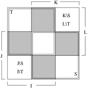
Breteaux chequerboard: The integrals vanish if $J\cup L\neq I\cup K$. $S:=J\cap K$ and $T:=I\cap L$. Grey areas represent empty subsets.

We go on in (19) and take the intersection $S\cap T$ into account. The term $\prod\limits_{\alpha\in T}\overline{\psi}_{\alpha}\psi_{\alpha}\prod\limits_{\alpha\in S}\left(1+\overline{\psi}_{\alpha}\psi_{\alpha}\right)$ contributes to the the integral as follows:

$$\prod\limits_{\alpha\in T\cup S}\frac{\delta}{\delta\overline{\psi}_{\alpha}}\frac{\delta}{\delta\psi_{\alpha}}\prod\limits_{\alpha\in T}\overline{\psi}_{\alpha}\psi_{\alpha}\prod\limits_{\beta\in S}\left(1+\overline{\psi}_{\beta}\psi_{\beta}\right)=\prod\limits_{\alpha\in T\cup S}\frac{\delta}{\delta\overline{\psi}_{\alpha}}\frac{\delta}{\delta\psi_{\alpha}}\prod\limits_{\alpha\in T\cup S}\overline{\psi}_{\alpha}\psi_{\alpha},$$

since $\prod\limits_{\alpha\in T\cap S}\overline{\psi}_{\alpha}\psi_{\alpha}\prod\limits_{\beta\in T\cap S}\left(1+\overline{\psi}_{\beta}\psi_{\beta}\right)=\prod\limits_{\alpha\in T\cap S}\overline{\psi}_{\alpha}\psi_{\alpha}$ and

$$\prod\limits_{\alpha\in S\backslash\left(T\cap S\right)}\frac{\delta}{\delta\overline{\psi}_{\alpha}}\frac{\delta}{\delta\psi_{\alpha}}\prod\limits_{\beta\in S\backslash\left(T\cap S\right)}\left(1+\overline{\psi}_{\beta}\psi_{\beta}\right)=\prod\limits_{\alpha\in S\backslash\left(T\cap S\right)}\frac{\delta}{\delta\overline{\psi}_{\alpha}}\frac{\delta}{\delta\psi_{\alpha}}\prod\limits_{\beta\in S\backslash\left(T\cap S\right)}\overline{\psi}_{\beta}\psi_{\beta}.$$

This finishes our calculations and we conclude:

$$\int\mathcal{D}(\overline{\Psi},\Psi)\,\mu\star\eta=\sigma_{S}\sigma_{T}\tilde{\sigma}\int\mathrm{d}(\overline{\Psi},\Psi)\,\prod\limits_{\alpha\in T\cup S}\overline{\psi}_{\alpha}\psi_{\alpha}$$

$$\qquad\qquad\qquad\qquad\qquad\times\prod\limits_{\begin{subarray}{c}\alpha\in M\\ \backslash\left(J\cup K\cup I\cup L\right)\end{subarray}}\left(1+2\overline{\psi}_{\alpha}\psi_{\alpha}\right)\overline{\Psi}_{I\backslash T}\overline{\Psi}_{K\backslash S}\Psi_{J\backslash S}\Psi_{L\backslash T}.$$ (20)

The r.h.s. of the assertion in Theorem 4.14 can be calculated analogously. The result is

$$\int\mathcal{D}(\overline{\Psi},\Psi)\,\eta\star\mu=\sigma_{T}\sigma_{S}\widehat{\sigma}\int\mathrm{d}(\overline{\Psi},\Psi)\,\prod\limits_{\alpha\in S\cup T}\overline{\psi}_{\alpha}\psi_{\alpha}$$

$$\qquad\qquad\qquad\qquad\qquad\times\prod\limits_{\begin{subarray}{c}\alpha\in M\\ \backslash\left(J\cup K\cup I\cup L\right)\end{subarray}}\left(1+2\overline{\psi}_{\alpha}\psi_{\alpha}\right)\overline{\Psi}_{K\backslash S}\overline{\Psi}_{I\backslash T}\Psi_{L\backslash T}\Psi_{J\backslash S},$$

where the sign resulting from the anticommutations is

$$\widehat{\sigma}:=\left(-1\right)^{|T||L\backslash T|+|S||L\backslash T|+\frac{1}{2}|S|\left(|S|-1\right)+\frac{1}{2}|T|\left(|T|-1\right)+|S||I\backslash T|+|S||K\backslash S|+|I\backslash T||L\backslash T|}.$$

The l.h.s. and the r.h.s. of Theorem 4.14 are symmetric with respect to the involved sets. The proof is complete by the observation

$$\tilde{\sigma}=\widehat{\sigma}=\left(-1\right)^{\frac{1}{2}|S|\left(|S|-1\right)+\frac{1}{2}|T|\left(|T|-1\right)+|K\backslash S||J\backslash S|+|T||K\backslash S|+|S||J\backslash S|},$$

which follows from $I\backslash T=J\backslash S$ and $L\backslash T=K\backslash S$. ∎

Remark 4.15.

The integral on the r.h.s. of (20) can be carried out. Abbreviating $s_{Q}:=\frac{1}{2}|Q|\left(|Q|-1\right)$ for $Q\subseteq M$, we have

$$\int\mathcal{D}(\overline{\Psi},\Psi)\,\mu\star\eta =\sigma_{S}\sigma_{T}\left(-1\right)^{s_{S}+s_{T}+|T||K\backslash S|+|S||J\backslash S|+s_{I\backslash T}+s_{K\backslash S}}$$

$$\qquad\times\int\mathrm{d}(\overline{\Psi},\Psi)\,\prod\limits_{\alpha\in I\backslash T}\overline{\psi}_{\alpha}\psi_{\alpha}\prod\limits_{\alpha\in K\backslash S}\overline{\psi}_{\alpha}\psi_{\alpha}\prod\limits_{\alpha\in T\cup S}\overline{\psi}_{\alpha}\psi_{\alpha}\prod\limits_{\alpha\in M\backslash\left(I\cup K\right)}\left(1+2\overline{\psi}_{\alpha}\psi_{\alpha}\right)$$

$$=\sigma_{S}\sigma_{T}\left(-1\right)^{s_{S}+s_{T}+|T||K\backslash S|+|S||J\backslash S|+s_{I\backslash T}+s_{K\backslash S}}$$

$$\qquad\times\left(-1\right)^{|I\backslash T|+|K\backslash S|+|T\cup S|}\left(-2\right)^{|M|-|I\cup K|}.$$

With $|I\backslash T|+|K\backslash S|+|T\cup S|=|I\cup K|$ we obtain

$$\int\mathcal{D}(\overline{\Psi},\Psi)\,\mu\star\eta=\sigma_{S}\sigma_{T}\left(-1\right)^{s_{J}+s_{L}}2^{|M|-|I\cup K|}$$

for $\mu:=\overline{\Psi}_{I}\Psi_{J}$ and $\eta:=\overline{\Psi}_{K}\Psi_{L}$.

Remark 4.16.

A consequence of Lemma 4.7 and 4.14 is the invariance of the Grassmann integral with respect to cyclic permutations of the integrand:

$$\int\mathrm{d}(\overline{\Psi},\Psi)\left(\mu_{1}\star\mu_{2}\star\cdots\star\mu_{N}\right)=\int\mathrm{d}(\overline{\Psi},\Psi)\left(\mu_{2}\star\cdots\star\mu_{N}\star\mu_{1}\right).$$ (21)

This also holds true for $\int\mathcal{D}(\overline{\Psi},\Psi)\left(\,\cdot\,\right)$, since $\mathrm{e}^{2\left(\overline{\Psi},\Psi\right)}$ commutes with any $\mu\in\mathcal{G}_{M}$.

Given an involution on $\left(\mathcal{G}_{M},+,\star\right)$, we define the property of positivity on $\mathcal{G}_{M}$ as follows.

Definition 4.17.

We call $\mu\in\mathcal{G}_{M}$ positive semi-definite, shortly $\mu\geq 0$, if there exists an $\eta\in\mathcal{G}_{M}$ such that

$$\mu=\eta^{*}\star\eta.$$

Approaching the problem of representability by Grassmann integration, an important result is the following theorem.

Theorem 4.18.

For any $\mu\in\mathcal{G}_{M}$ with $\mu\geq 0$ we have

$$\left(-1\right)^{|M|}\int\mathcal{D}(\overline{\Psi},\Psi)\,\mu\geq 0.$$ (22)

Proof.

We use an induction in $|M|\in\mathbbm{N}$. For this purpose, we write any $\xi\in\mathcal{G}_{M+1}:=\mathrm{span}\left\{\overline{\psi}_{1},\dots,\overline{\psi}_{|M|},\overline{\psi}_{|M|+1},\psi_{1},\dots,\psi_{|M|},\psi_{|M|+1}\right\}$ as

$$\xi=\eta_{00}+\eta_{01}\psi_{|M|+1}+\overline{\psi}_{|M|+1}\eta_{10}+\overline{\psi}_{|M|+1}\eta_{11}\psi_{|M|+1}$$ (23)

for normal-ordered $\eta_{00},\,\eta_{01},\,\eta_{10},\,\eta_{11}\in\mathcal{G}_{M}$. We indicate integration with respect to a certain index set $M$ by writing $\int\mathrm{d}_{M}(\overline{\Psi},\Psi)$ and $\int\mathcal{D}_{M}(\overline{\Psi},\Psi)$, respectively. Furthermore, we recall that

$$\mathrm{e}^{E_{M}} :=\mathrm{e}^{\left(\overline{\Psi},\Psi\right)}\mathrm{e}^{\left(\overline{\Psi},\Phi\right)}\mathrm{e}^{-\left(\overline{\Phi},\Phi\right)}\mathrm{e}^{\left(\overline{\Phi},\Psi\right)}$$

$$=\prod\limits_{\alpha=1}^{M}\left(1-\overline{\phi}_{\alpha}\phi_{\alpha}+\overline{\psi}_{\alpha}\psi_{\alpha}+\overline{\phi}_{\alpha}\psi_{\alpha}+\overline{\psi}_{\alpha}\phi_{\alpha}-2\overline{\psi}_{\alpha}\psi_{\alpha}\overline{\phi}_{\alpha}\phi_{\alpha}\right).$$

In order to show (22) for $|M|=0$, we consider $\mu:=a^{*}\star a\in\mathcal{G}_{0}$ with $a\in\mathbbm{C}$, and observe that with $\int\mathcal{D}_{0}(\overline{\Psi},\Psi)=1$ the l.h.s. of (22) is nonnegative,

$$\int\mathcal{D}_{0}(\overline{\Psi},\Psi)\,\mu=\left|a\right|^{2}\geq 0.$$

Now we assume that (22) holds for $|M|$ and consider the l.h.s. of (22) for $|M|+1$ and $\mu=\xi^{*}\star\xi$. We abbreviate $\psi_{|M|+1}\equiv\psi^{\prime}$ and $\overline{\psi}_{|M|+1}\equiv\overline{\psi^{\prime}}$.

$$\left(-1\right)^{|M|+1}\int\mathcal{D}_{M+1}(\overline{\Psi},\Psi)\left(\xi^{*}\star\xi\right)$$

$$\qquad=\left(-1\right)^{|M|+1}\int\mathcal{D}_{M+1}(\overline{\Psi},\Psi)\Big{[}\eta_{00}^{*}\star\eta_{00}+\eta_{00}^{*}\star\left(\overline{\psi^{\prime}}\,\eta_{11}\psi^{\prime}\right)+\left(\overline{\psi^{\prime}}\,\eta_{01}^{*}\right)\star\left(\eta_{01}\psi^{\prime}\right)\big{.}$$

$$\phantom{....................}+\left(\eta_{10}^{*}\psi^{\prime}\right)\star\left(\overline{\psi^{\prime}}\,\eta_{10}\right)+\left(\overline{\psi^{\prime}}\,\eta_{11}^{*}\psi^{\prime}\,\right)\star\eta_{00}\big{.}+\left(\overline{\psi^{\prime}}\,\eta_{11}^{*}\psi^{\prime}\right)\star\left(\overline{\psi^{\prime}}\,\eta_{11}\psi^{\prime}\right)\Big{]}.$$ (24)

Other terms like $\int\mathcal{D}_{M+1}(\overline{\Psi},\Psi)\eta_{00}^{*}\star\left(\eta_{01}\psi^{\prime}\right)$ vanish, as can be seen in (19), since, in this case, $I\cup K\neq J\cup L$.

In the next step, we use the definition of the star product and the identity $\int\mathrm{d}_{M+1}(\overline{\Psi},\Psi)=\int\mathrm{d}_{M}(\overline{\Psi},\Psi)\frac{\delta}{\delta\overline{\psi^{\prime}}}\frac{\delta}{\delta\psi^{\prime}}$ to carry out all integrations with respect to $\psi^{\prime}$ and $\overline{\psi^{\prime}}$. We exemplify this step by the last term on the r.h.s. of (24):

$$\left(-1\right)^{|M|+1}\int\mathcal{D}_{M+1}(\overline{\Psi},\Psi)\left(\overline{\psi^{\prime}}\,\eta_{11}^{*}\psi^{\prime}\right)\star\left(\overline{\psi^{\prime}}\,\eta_{11}\psi^{\prime}\right)$$

$$\qquad=\left(-1\right)^{|M|+1}\int\mathrm{d}_{M+1}(\overline{\Psi},\Psi)\int\mathrm{d}_{M+1}\left(\overline{\Phi},\Phi\right)\overline{\psi^{\prime}}\,\eta_{11}^{*}\left(\overline{\psi},\phi\right)\phi^{\prime}\overline{\phi^{\prime}}\,\eta_{11}\left(\overline{\phi},\psi\right)\psi^{\prime}\,\mathrm{e}^{E_{M+1}}.$$

Since $\eta_{11}^{*}\left(\overline{\psi},\phi\right)\eta_{11}\left(\overline{\phi},\psi\right)$ is even in the $\left(\overline{\psi},\psi,\overline{\phi},\phi\right)$ variables, we continue with

$$\left(-1\right)^{|M|+1}\int\mathcal{D}_{M+1}(\overline{\Psi},\Psi)\left(\overline{\psi^{\prime}}\,\eta_{11}^{*}\psi^{\prime}\right)\star\left(\overline{\psi^{\prime}}\,\eta_{11}\psi^{\prime}\right)$$

$$\qquad=\left(-1\right)^{|M|+1}\int\mathrm{d}_{M}(\overline{\Psi},\Psi)\int\mathrm{d}_{M}\left(\overline{\Phi},\Phi\right)\eta_{11}^{*}\left(\overline{\psi},\phi\right)\eta_{11}\left(\overline{\phi},\psi\right)\mathrm{e}^{E_{M}}$$

$$\qquad\quad\times\frac{\delta}{\delta\overline{\phi^{\prime}}}\frac{\delta}{\delta\phi^{\prime}}\frac{\delta}{\delta\overline{\psi^{\prime}}}\frac{\delta}{\delta\psi^{\prime}}\overline{\psi^{\prime}}\phi^{\prime}\overline{\phi^{\prime}}\psi^{\prime}\left(1-\overline{\phi^{\prime}}\phi^{\prime}+\overline{\psi^{\prime}}\psi^{\prime}+\overline{\phi^{\prime}}\psi^{\prime}+\overline{\psi^{\prime}}\phi^{\prime}-2\overline{\psi^{\prime}}\psi^{\prime}\overline{\phi^{\prime}}\phi^{\prime}\right)$$

$$\qquad=\left(-1\right)^{|M|+2}\int\mathcal{D}_{M}(\overline{\Psi},\Psi)\,\eta_{11}^{*}\star\eta_{11}.$$

By analogous calculations, we obtain

$$\left(-1\right)^{|M|+1}\int\mathcal{D}_{M+1}(\overline{\Psi},\Psi)\left(\xi^{*}\star\xi\right)$$

$$\qquad=\left(-1\right)^{|M|+2}\int\mathcal{D}_{M}(\overline{\Psi},\Psi)\Big{[}2\eta_{00}^{*}\star\eta_{00}+\eta_{00}^{*}\star\tilde{\eta}_{11}+\eta_{01}^{*}\star\eta_{01}+\eta_{10}^{*}\star\eta_{10}$$

$$\phantom{....................................................................................}+\tilde{\eta}_{11}^{*}\star\eta_{00}+\eta_{11}^{*}\star\eta_{11}\Big{]},$$

where $\tilde{\eta}_{11}:=\sum\limits_{I,J}\left(-1\right)^{|I|+|J|}a_{IJ}\overline{\Psi}_{I}\Psi_{J}\in\mathcal{G}_{M}$ if $\eta_{11}:=\sum\limits_{I,J}a_{IJ}\overline{\Psi}_{I}\Psi_{J}$ for some $a_{IJ}\in\mathbbm{C}$. $\tilde{\eta}_{11}$ occurs due to the anticommutations of $\psi_{M+1}$ with $\eta_{11}^{*}$ and of $\overline{\psi}_{M+1}$ with $\eta_{11}$ in the second and the fifth term on the r.h.s. of (24), respectively. Observing that

$$\int\mathcal{D}_{M}(\overline{\Psi},\Psi)\,\tilde{\eta}_{11}^{*}\star\tilde{\eta}_{11}$$

$$\qquad=\sum\limits_{I,J,K,L}a_{IJ}\overline{a}_{LK}\left(-1\right)^{|I|+|J|+|K|+|L|}\int\mathcal{D}_{M}(\overline{\Psi},\Psi)\left(\overline{\Psi}_{I}\Psi_{J}\right)\star\left(\overline{\Psi}_{K}\Psi_{L}\right)$$

$$\qquad=\int\mathcal{D}_{M}(\overline{\Psi},\Psi)\,\eta_{11}^{*}\star\eta_{11},$$

since $|I|+|J|+|K|+|L|$ is even (otherwise both integrals vanish), we finally conclude

$$\left(-1\right)^{|M|+1}\int\mathcal{D}_{M+1}(\overline{\Psi},\Psi)\left(\xi^{*}\star\xi\right)$$

$$\qquad=\left(-1\right)^{|M|+2}\int\mathcal{D}_{M}(\overline{\Psi},\Psi)\Big{[}\eta_{00}^{*}\star\eta_{00}+\left(\eta_{00}+\tilde{\eta}_{11}\right)^{*}\star\left(\eta_{00}+\tilde{\eta}_{11}\right)+\eta_{01}^{*}\star\eta_{01}+\eta_{10}^{*}\star\eta_{10}\Big{]},$$

which is non-negative by the induction hypothesis. ∎

Finally, we can express the trace of an operator of $\mathcal{B}\left(\wedge\mathcal{H}\right)$ and, thanks to Lemma 4.10, the trace of a product of such operators as a Grassmann integral.

Theorem 4.19.

For all $A\in\mathcal{B}\left(\wedge\mathcal{H}\right)$ we have

$$\mathrm{tr}_{\wedge\mathcal{H}}\left\{A\right\}=\left(-1\right)^{|M|}\int\mathcal{D}(\overline{\Psi},\Psi)\,\Theta\left(A\right).$$ (25)

Proof.

We assume that $A\in\mathcal{B}\left(\wedge\mathcal{H}\right)$ is normal-ordered. Due to the linearity of the trace and the Grassmann integral it suffices to consider $\mathrm{tr}_{\wedge\mathcal{H}}\left\{{c}^{*}_{i_{1}}\cdots{c}^{*}_{i_{m}}{c}_{j_{1}}\cdots{c}_{j_{n}}\right\}$, where $I:=\left\{i_{1},\dots,i_{m}\right\}$ and $J:=\left\{j_{1},\dots,j_{n}\right\}$ are ordered. For $I\neq J$, both the l.h.s. and the r.h.s. of (25) vanish. For $I=J$, the l.h.s. of (25) is given by

$$\mathrm{tr}_{\wedge\mathcal{H}}\left\{{c}^{*}_{i_{1}}\cdots{c}^{*}_{i_{m}}{c}_{i_{1}}\cdots{c}_{i_{m}}\right\}=\left(-1\right)^{\frac{1}{2}|I|\left(|I|-1\right)}2^{|M|-|I|}.$$

On the r.h.s. of (25) we have $\Theta\left({c}^{*}_{i_{1}}\cdots{c}^{*}_{i_{m}}{c}_{i_{1}}\cdots{c}_{i_{m}}\right)=\overline{\psi}_{i_{1}}\cdots\overline{\psi}_{i_{m}}\psi_{i_{1}}\cdots\psi_{i_{m}}$ and, thus,

$$\int\mathcal{D}(\overline{\Psi},\Psi)\,\overline{\psi}_{i_{1}}\cdots\overline{\psi}_{i_{m}}\psi_{i_{1}}\cdots\psi_{i_{m}} =\left(-1\right)^{\frac{1}{2}|I|\left(|I|+1\right)}\int\mathcal{D}(\overline{\Psi},\Psi)\,\prod\limits_{\alpha=1}^{m}\left(\psi_{i_{\alpha}}\overline{\psi}_{i_{\alpha}}\right)$$

$$=\left(-1\right)^{|M|}\left(-1\right)^{\frac{1}{2}|I|\left(|I|+1\right)}2^{|M|-|I|},$$

since $\prod\limits_{\alpha\in I}\left(\psi_{\alpha}\overline{\psi}_{\alpha}\right)\mathrm{e}^{2\left(\overline{\Psi},\Psi\right)}=\prod\limits_{\alpha\in I}\left(\psi_{\alpha}\overline{\psi}_{\alpha}\right)\prod\limits_{\alpha\in M\backslash I}\left(1+2\overline{\psi}_{\alpha}\psi_{\alpha}\right)$ and, therefore,

$$\prod\limits_{\alpha\in M}\left(\frac{\delta}{\delta\overline{\psi}}\frac{\delta}{\delta\psi}\right)\prod\limits_{\alpha\in I}\left(\psi_{\alpha}\overline{\psi}_{\alpha}\right)\mathrm{e}^{2\left(\overline{\Psi},\Psi\right)}=\left(-2\right)^{|M|-|I|}.$$

The proof is complete by $\left(-2\right)^{|M|-|I|}=\left(-1\right)^{|M|}\left(-1\right)^{|I|}2^{|M|-|I|}$. ∎

Due to the restriction to a Hilbert space with even dimension, we henceforth skip the factor $\left(-1\right)^{|M|}$.

5 Representability Conditions from Grassmann Integrals

The last section allows for an application of the Grassmann integration on the problem of representability for fermion systems. In particular, we are interested in necessary conditions for the 1- and 2-pdm to have their origin in a density matrix $\rho$ [2]. In the language of Grassmann integration we call the equivalents of density matrices Grassmann densities.

Definition 5.1.

A Grassmann variable $\vartheta^{*}\star\vartheta\in\mathcal{G}_{M}$ is called Grassmann density if it is normalized, i.e., fulfills

$$\int\mathcal{D}\left(\overline{\Psi},\Psi\right)\vartheta^{*}\star\vartheta\,=1.$$

By definition, the Grassmann density is positive semi-definite and self-adjoint. For a given state $\rho$, the map $\Theta$ immediately provides $\vartheta^{*}\star\vartheta$, namely $\vartheta^{*}\star\vartheta=\Theta\left(\rho\right)$. Thanks to the product rule for $\Theta$ and the positive semi-definiteness of $\rho$, we also have $\vartheta^{*}\star\vartheta=\Theta\big{(}\rho^{\frac{1}{2}}\rho^{\frac{1}{2}}\big{)}=\Theta\big{(}\rho^{\frac{1}{2}}\big{)}\star\Theta\big{(}\rho^{\frac{1}{2}}\big{)}$. $\Theta$ is a bijection and compatible with the involution. This implies that $\vartheta=\Theta\big{(}\rho^{\frac{1}{2}}\big{)}$. Given a Grassmann density, we can formulate the problem of representability by Grassmann integrals using the trace-formula (25).

Definition 5.2.

Let $\left\{\overline{\psi}_{i},\psi_{i}\right\}_{i\in M}$ be the generators of $\mathcal{G}_{M}$ and associate $\left\{\psi_{i}\right\}_{i\in M}$ with a fixed ONB of $\mathcal{H}$. The 1-pdm $\gamma_{\vartheta}\in\mathcal{B}\left(\mathcal{H}\right)$ and 2-pdm $\Gamma_{\vartheta}\in\mathcal{B}\left(\mathcal{H}\otimes\mathcal{H}\right)$ of a Grassmann density $\vartheta^{*}\star\vartheta$ are defined by their matrix elements:

$$\left<\psi_{k},\gamma_{\vartheta}\psi_{l}\right> :=\int\mathcal{D}(\overline{\Psi},\Psi)\,\vartheta^{*}\star\vartheta\star\overline{\psi}_{l}\star\psi_{k}\,\quad\text{and}$$ (26)

$$\left<\psi_{m}\otimes\psi_{n},\Gamma_{\vartheta}\left(\psi_{l}\otimes\psi_{k}\right)\right> :=\int\mathcal{D}\left(\overline{\Psi},\Psi\right)\vartheta^{*}\star\vartheta\star\overline{\psi}_{k}\star\overline{\psi}_{l}\star\psi_{m}\star\psi_{n}\,.$$ (27)

Applying the trace formula (25) on (26) and (27), respectively, we observe that

$$\left<\psi_{k},\gamma_{\rho}\psi_{l}\right> =\mathrm{tr}_{\wedge\mathcal{H}}\left\{\Theta^{-1}\left(\vartheta^{*}\star\vartheta\right){c}^{*}_{l}{c}_{k}\right\}\quad\text{and}$$

$$\left<\psi_{m}\otimes\psi_{n},\Gamma_{\rho}\left(\psi_{l}\otimes\psi_{k}\right)\right> =\mathrm{tr}_{\wedge\mathcal{H}}\left\{\Theta^{-1}\left(\vartheta^{*}\star\vartheta\right){c}^{*}_{l}{c}^{*}_{k}{c}_{n}{c}_{m}\right\},$$

which agrees with the common definition of the 1- and 2-pdm [2] if we interpret $\Theta^{-1}\left(\vartheta^{*}\star\vartheta\right)=\left(\Theta^{-1}\left(\vartheta\right)\right)^{*}\Theta^{-1}\left(\vartheta\right)$ as a density matrix $\rho\in\mathcal{B}\left(\wedge\mathcal{H}\right)$. The problem of representability can be formulated as follows:

Definition 5.3.

We call $\left(\gamma,\Gamma\right)\in\mathcal{B}\left(\mathcal{H}\right)\times\mathcal{B}\left(\mathcal{H}\otimes\mathcal{H}\right)$ representable if there exists a Grassmann density $\vartheta^{*}\star\vartheta$ such that $\left(\gamma,\Gamma\right)=\left(\gamma_{\vartheta},\Gamma_{\vartheta}\right)$.

5.1 Conditions on the One-Particle Density Matrix

The lower and upper bound for the eigenvalues of the 1-pdm $\gamma_{\vartheta}$ of a Grassmann state $\vartheta^{*}\star\vartheta$ arise directly from the definition of the 1-pdm (see [2] for further details). Here, we would like to derive the conditions by Grassmann integration. To this end, we consider certain subspaces of $\mathcal{G}_{M}$.

Definition 5.4.

For any $n\in\mathbbm{N}$, $n\leq|M|$, we define the subspace

$$\mathcal{G}_{M}^{(n)}:=\mathrm{span}\left\{\overline{\Psi}_{I}\Psi_{J}|\ |I|,|J|\leq n\right\}\subseteq\mathcal{G}_{M}.$$

Bounds for the 1-pdm rise by considering $\mathcal{G}_{M}^{(1)}$. In what follows, we call conditions derived by considering $\mathcal{G}_{M}^{(n)}$ as conditions of $n$-th order.

Lemma 5.5.

Theorem 4.18 implies

$$\gamma_{\vartheta}\geq 0.$$

Proof.

Let $\left\{\overline{\psi}_{i},\psi_{i}\right\}_{i\in M}$ be the generators of $\mathcal{G}_{M}$ and $\alpha_{k}\in\mathbbm{C}\ \forall\,k\in M$. In Theorem 4.18, we make use of Equation (21) with $\eta:=\phi\star\vartheta^{*}$ and $\phi:=\sum\limits_{k\in M}\alpha_{k}\psi_{k}\in\mathcal{G}_{M}$. We observe that, according to the involution $\left(\,\cdot\,\right)^{*}$ on $\mathcal{G}_{M}$, $\phi^{*}=\sum\limits_{k\in M}\overline{\alpha}_{k}\overline{\psi}_{k}$, and $\eta^{*}=\left(\phi\star\vartheta^{*}\right)^{*}=\vartheta\star\phi^{*}$. This leads to

$$0 \leq\int\mathcal{D}(\overline{\Psi},\Psi)\,\eta^{*}\star\eta\,$$

$$=\sum\limits_{k,l\in M}\overline{\alpha}_{k}\alpha_{l}\int\mathcal{D}(\overline{\Psi},\Psi)\,\vartheta^{*}\star\vartheta\star\overline{\psi}_{k}\star\psi_{l}\,$$

$$=\left<f,\gamma_{\vartheta}f\right>,$$

where $f:=\sum\limits_{i\in M}\overline{\alpha}_{i}\psi_{i}\in\mathcal{H}$ is arbitrary. ∎

The upper bound for $\gamma_{\vartheta}$ is given by another choice of $\eta$.

Lemma 5.6.

Theorem 4.18 implies

$$\gamma_{\vartheta}\leq\mathbbm{1}.$$

Proof.

The bound can be proven by following the steps of the proof of the lower bound. Again, we have $\alpha_{k}\in\mathbbm{C}\ \forall\,k\in M$ and set $\phi^{*}=\sum\limits_{k\in M}\overline{\alpha}_{k}\overline{\psi}_{k}\in\mathcal{G}_{M}$ and, this time, $\eta^{*}=\left(\phi^{*}\star\vartheta\right)^{*}=\vartheta^{*}\star\phi$. Before we go on, we observe that by the CAR on $\mathcal{G}_{M}$ given in (4.8),

$$\phi\star\phi^{*} =\sum\limits_{k,l\in M}\alpha_{k}\overline{\alpha}_{l}\psi_{k}\star\overline{\psi}_{l}=\sum\limits_{k\in M}\overline{\alpha}_{k}\alpha_{k}-\sum\limits_{k,l\in M}\alpha_{k}\overline{\alpha}_{l}\overline{\psi}_{l}\star\psi_{k}.$$

Inserting this into the inequality of Theorem 4.18 and using the associativity of the star product, we obtain

$$0 \leq\int\mathcal{D}(\overline{\Psi},\Psi)\,\eta^{*}\star\eta\,$$

$$=\sum\limits_{k\in M}\left|\alpha_{k}\right|^{2}-\sum\limits_{k,l\in M}\overline{\alpha}_{l}\alpha_{k}\int\mathcal{D}(\overline{\Psi},\Psi)\,\vartheta^{*}\star\vartheta\star\overline{\psi}_{l}\star\psi_{k}\,$$

$$=\left<g,\left(\mathbbm{1}-\gamma_{\vartheta}\right)g\right>,$$

where we have used $\int\mathcal{D}(\overline{\Psi},\Psi)\,\vartheta^{*}\star\vartheta\,=1$ and $g:=\sum\limits_{k\in M}\overline{\alpha}_{k}\psi_{k}\in\mathcal{H}$. ∎

Considering the subspace $\mathcal{G}_{M}^{(1)}$, we can summarize our last two results.

Theorem 5.7.

Let $\vartheta\star\vartheta^{*}$ be a Grassmann density and $\gamma_{\vartheta}$ its 1-pdm. Then the following statements are equivalent:

• $0\leq\gamma_{\vartheta}\leq\mathbbm{1}$.

• $\forall\mu\in\mathcal{G}_{M}^{(1)}$: $\int\mathcal{D}(\overline{\Psi},\Psi)\,\vartheta^{*}\star\vartheta\star\mu\geq 0$.

Proof.

In Theorem 3.1 of [2], the analogue of this theorem has been shown for polynomials in creation and annihilation operators of degree lower than or equal to two. Thanks to the bijection $\Theta$, we have a one-to-one mapping between the space of polynomials of degree lower than or equal to two and $\mathcal{G}_{M}^{(1)}$. ∎

5.2 G-, P-, and Q-Condition

We proceed with representability conditions of second order by considering $\mathcal{G}_{M}^{(2)}$ and a star-product of $\overline{\psi}$ and $\psi$, in this case, for example $\phi:=\sum\limits_{k,l\in M}\alpha_{kl}\psi_{k}\star\psi_{l}\in\mathcal{G}_{M}$ with $\alpha_{kl}\in\mathbbm{C}\ \forall\,k,l\in M$. This time, we are interested in conditions on $\Gamma_{\vartheta}$ and use the Grassmann integration to rewrite the matrix elements of the 2-pdm as in (27). The first condition is the P-Condition.

Lemma 5.8.

Theorem 4.18 implies the P-Condition

$$\Gamma_{\vartheta}\geq 0.$$

Proof.

The proof is similar to the one in the last subsection. Setting $\phi:=\sum\limits_{k,l\in M}\alpha_{kl}\psi_{k}\star\psi_{l}\in\mathcal{G}_{M}$ with $\alpha_{kl}\in\mathbbm{C}\ \forall\,k,l\in M$, $\eta:=\phi\star\vartheta^{*}$, and $\eta^{*}=\left(\phi\star\vartheta^{*}\right)^{*}=\vartheta\star\phi^{*}$, we arrive at

$$0 \leq\int\mathcal{D}(\overline{\Psi},\Psi)\,\eta^{*}\star\eta\,$$

$$=\sum\limits_{k,l,m,n\in M}\overline{\alpha}_{kl}\alpha_{mn}\int\mathcal{D}(\overline{\Psi},\Psi)\,\vartheta^{*}\star\vartheta\star\overline{\psi}_{l}\star\overline{\psi}_{k}\star\psi_{m}\star\psi_{n}\,$$

$$=\left<F,\Gamma_{\vartheta}F\right>,$$ (28)

where $F:=\sum\limits_{k,l\in M}\overline{\alpha}_{kl}\left(\psi_{m}\otimes\psi_{n}\right)\in\mathcal{H}\otimes\mathcal{H}$ is arbitrary. ∎

The Q-Condition is the next representability condition. In order to obtain a convenient formulation of this condition, we use an exchange operator on $\mathcal{B}\left(\mathcal{H}\otimes\mathcal{H}\right)$ which is defined by $\mathrm{Ex}\left(f\otimes g\right):=g\otimes f$ for $f,g\in\mathcal{H}$.

Lemma 5.9.

Theorem 4.18 implies the Q-Condition

$$\Gamma_{\vartheta}+\left(\mathbbm{1}-\mathrm{Ex}\right)\left(\mathbbm{1}\otimes\mathbbm{1}-\gamma_{\vartheta}\otimes\mathbbm{1}-\mathbbm{1}\otimes\gamma_{\vartheta}\right)\geq 0.$$

Proof.

With $\phi:=\sum\limits_{k,l\in M}\overline{\alpha}_{kl}\overline{\psi}_{k}\star\overline{\psi}_{l}\in\mathcal{G}_{M}$, $\alpha_{kl}\in\mathbbm{C}\ \forall\,k,l\in M$, and $\eta=\phi\star\vartheta^{*}$, we have

$$0 \leq\int\mathcal{D}(\overline{\Psi},\Psi)\,\eta^{*}\star\eta\,$$

$$=\sum\limits_{k,l,m,n\in M}\overline{\alpha}_{kl}\alpha_{mn}\int\mathcal{D}(\overline{\Psi},\Psi)\,\vartheta^{*}\star\vartheta\star\psi_{n}\star\psi_{m}\star\overline{\psi}_{k}\star\overline{\psi}_{l}.$$

Aiming for an expression in terms of $\Gamma$ and $\gamma$, we establish normal ordering using the CAR:

$$\psi_{n}\star\psi_{m}\star\overline{\psi}_{k}\star\overline{\psi}_{l} =\delta_{mk}\delta_{nl}-\delta_{nk}\delta_{ml}+\delta_{nk}\overline{\psi}_{l}\star\psi_{m}-\delta_{mk}\overline{\psi}_{l}\star\psi_{n}+\delta_{nl}\overline{\psi}_{k}\star\psi_{l}$$

$$\phantom{=}-\delta_{ml}\overline{\psi}_{k}\star\psi_{n}-\overline{\psi}_{k}\star\overline{\psi}_{l}\star\psi_{n}\star\psi_{m}.$$ (29)

As in the proof of Lemma 5.8, we write an arbitrary $G\in\mathcal{H}\otimes\mathcal{H}$ as $G:=\sum\limits_{k,l\in M}\alpha_{kl}\left(\psi_{k}\otimes\psi_{l}\right)$ for some $\alpha_{kl}\in\mathbbm{C}$. Hence, $\sum\limits_{k,l,m,n\in M}\overline{\alpha}_{kl}\alpha_{mn}\delta_{km}\delta_{ln}=\left<G,\mathbbm{1}\,G\right>$ and $\sum\limits_{k,l,m,n\in M}\overline{\alpha}_{kl}\alpha_{mn}\delta_{kn}\delta_{lm}=\left<G,\mathrm{Ex}\,G\right>$. With (26) and (27), we find

$$0\leq\left<G,\left(\Gamma_{\vartheta}+\left(\mathbbm{1}-\mathrm{Ex}\right)\left(\mathbbm{1}\otimes\mathbbm{1}-\gamma_{\vartheta}\otimes\mathbbm{1}-\mathbbm{1}\otimes\gamma_{\vartheta}\right)\right)G\right>$$

by evaluating the Grassmann integral $\int\mathcal{D}(\overline{\Psi},\Psi)\left(\,\cdot\,\right)$ on the r.h.s. of (29). ∎

The last second order representability condition which can be derived by the described method is the (optimal) G-Condition. Deriving this condition by Grassmann integration requires a choice of $\eta$, that is not as obvious as before. In the following, $\mathrm{tr}_{1}\left\{\,\cdot\,\right\}$ denotes the trace on $\mathcal{H}$ and $\mathrm{tr}_{2}\left\{\,\cdot\,\right\}$ the trace on $\mathcal{H}\otimes\mathcal{H}$.

Lemma 5.10.

Theorem 4.18 implies the G-Condition:

$$\forall\,A\in\mathcal{B}\left(\mathcal{H}\right):\ \mathrm{tr}_{2}\left\{\left(A^{*}\otimes A\right)\left(\Gamma_{\vartheta}+\mathrm{Ex}\left(\gamma_{\vartheta}\otimes\mathbbm{1}\right)\right)\right\}\geq\left|\mathrm{tr}_{1}\left\{A\gamma_{\vartheta}\right\}\right|^{2}.$$ (30)

Proof.

This time, we choose $\eta:=\bigg{(}\sum\limits_{k,l\in M}\alpha_{kl}\overline{\psi}_{k}\star\psi_{l}-c\bigg{)}\star\vartheta$ with $c:=\sum\limits_{k,l\in M}\alpha_{kl}\int\mathcal{D}(\overline{\Psi},\Psi)\,\vartheta^{*}\star\vartheta\star\overline{\psi}_{k}\star\psi_{l}$ and $\alpha_{kl}\in\mathbbm{C}\ \forall\,k,l\in M$. Before we apply Theorem 4.18, we emphasize that by the CAR

$$\bigg{(}\sum\limits_{k,l\in M}\alpha_{kl}\overline{\psi}_{k}\psi_{l}-c\bigg{)}^{*}\star\bigg{(}\sum\limits_{k,l\in M}\alpha_{kl}\overline{\psi}_{k}\psi_{l}-c\bigg{)}$$

$$\quad\qquad\qquad=\overline{c}c-c\sum\limits_{k,l\in M}\overline{\alpha}_{kl}\overline{\psi}_{l}\star\psi_{k}-\overline{c}\sum\limits_{m,n\in M}\alpha_{mn}\overline{\psi}_{m}\star\psi_{n}$$

$$\qquad\qquad\qquad\quad-\sum\limits_{k,l\in M}\overline{\alpha}_{kl}\alpha_{mn}\overline{\psi}_{l}\star\overline{\psi}_{m}\star\psi_{k}\star\psi_{n}+\sum\limits_{k,l,n\in M}\overline{\alpha}_{kl}\alpha_{kn}\overline{\psi}_{l}\star\psi_{n}.$$ (31)

We consider the last two lines separately and integrate. The integration of the line before the last line in (31) yields

$$\int\mathcal{D}(\overline{\Psi},\Psi)\,\vartheta^{*}\star\vartheta\star\bigg{(}\overline{c}c-c\sum\limits_{k,l\in M}\overline{\alpha}_{kl}\overline{\psi}_{l}\star\psi_{k}-\overline{c}\sum\limits_{m,n\in M}\alpha_{mn}\overline{\psi}_{m}\star\psi_{n}\bigg{)}$$

$$\qquad\qquad\quad=\overline{c}c-c\overline{c}-\overline{c}c=-\overline{c}c,$$ (32)

which follows from the definition of $c$. It is important to notice that $c$ does not depend on $\psi$ or $\overline{\psi}$ and, therefore, is a constant with respect to the Grassmann integration. In detail, we have for $c$:

$$c=\sum\limits_{k,l\in M}\alpha_{kl}\int\mathcal{D}(\overline{\Psi},\Psi)\,\vartheta^{*}\star\vartheta\star\overline{\psi}_{k}\star\psi_{l}=\mathrm{tr}_{1}\left\{A\gamma_{\vartheta}\right\},$$ (33)

if we set $\left<\psi_{k},A\psi_{l}\right>:=\alpha_{kl}$ for every $k,l\in M$ and $A\in\mathcal{B}\left(\mathcal{H}\right)$. The evaluation of the Grassmann integral of the last line in (31) provides

$$-\sum\limits_{k,l\in M}\overline{\alpha}_{kl}\alpha_{mn}\int\mathcal{D}(\overline{\Psi},\Psi)\,\vartheta^{*}\star\vartheta\star\overline{\psi}_{l}\star\overline{\psi}_{m}\star\psi_{k}\star\psi_{n}\,$$

$$\qquad+\sum\limits_{k,l,n\in M}\overline{\alpha}_{kl}\alpha_{kn}\int\mathcal{D}(\overline{\Psi},\Psi)\,\vartheta^{*}\star\vartheta\star\overline{\psi}_{l}\star\psi_{n}\,$$

$$\qquad\qquad\qquad=\mathrm{tr}_{2}\left\{\left(A^{*}\otimes A\right)\left(\Gamma_{\vartheta}+\mathrm{Ex}\left(\gamma_{\vartheta}\otimes\mathbbm{1}\right)\right)\right\}.$$ (34)

Summing up, calculation (32) together with (33) and (34) gives

$$\mathrm{tr}_{2}\left\{\left(A^{*}\otimes A\right)\left(\Gamma_{\vartheta}+\mathrm{Ex}\left(\gamma_{\vartheta}\otimes\mathbbm{1}\right)\right)\right\}-\left|\mathrm{tr}_{1}\left\{A\gamma_{\vartheta}\right\}\right|^{2}\geq 0,$$

according to Theorem 4.18. ∎

We summarize our results using $\mathcal{G}_{M}^{(2)}$:

Theorem 5.11.

Let $\vartheta\star\vartheta^{*}$ be a Grassmann density, $\gamma_{\vartheta}$ its 1-pdm, and $\Gamma_{\vartheta}$ its 2-pdm. Then the following statements are equivalent:

• $\left(\gamma_{\vartheta},\Gamma_{\vartheta}\right)$ fulfills $0\leq\gamma_{\vartheta}\leq\mathbbm{1}$ and the G-, P-, and Q-Conditions.

• $\forall\mu\in\mathcal{G}_{M}^{(2)}$: $\int\mathcal{D}(\overline{\Psi},\Psi)\,\vartheta^{*}\star\vartheta\star\mu\geq 0$.

Proof.

Again, we use Theorem 3.1 of [2] and the bijection property of $\Theta$, which ensures that the space of polynomials of degree lower or equal than four in creation and annihilation operators is mapped one-to-on to $\mathcal{G}_{M}^{(2)}$. ∎

5.3 $\mathrm{T}_{1}$- and Generalized $\mathrm{T}_{2}$-Condition

The last sections imply that further conditions on $\gamma_{\vartheta}$ and $\Gamma_{\vartheta}$ can be found by taking into account monomials of higher order of the form $\overline{\psi}_{i_{1}}\star\cdots\star\overline{\psi}_{i_{n}}\star\psi_{j_{1}}\star\cdots\star\psi_{j_{n}}$ for $n>2$. Here we face the problem that monomials with $n>2$ have to “decompose” into monomials with $n\leq 2$. Due to this, only some choices of higher order monomials are suitable to derive further representability conditions. One of such monomials is given by

$$\tau_{1}:=\sum\limits_{i,j,k\in M}T_{ijk}\psi_{i}\star\psi_{j}\star\psi_{k}\in\mathcal{G}_{M},$$

Where $T_{ijk}\in\mathbbm{C}$ is, due to $\left\{\psi_{i},\psi_{j}\right\}_{\star}=0$, totally antisymmetric, i.e., $T_{ijk}=-T_{jik}=T_{jki}$. The $\mathrm{T}_{1}$-Condition is the following.

Theorem 5.12.

Let $T_{q}\in\mathcal{B}\left(\mathcal{H}\right)$ be trace class, and set $F_{T_{q}}:=\sum\limits_{k,n\in M}\overline{T}_{kqn}\left(\varphi_{k}\otimes\varphi_{n}\right)\in\mathcal{H}\otimes\mathcal{H}$, $T_{kqn}:=\left[T_{q}\right]_{kn}$. Then Theorem 4.18 implies the $\mathrm{T}_{1}$-Condition:

$$\sum\limits_{q\in M}\left(2\mathrm{tr}_{1}\left\{\left|T_{q}\right|^{2}\right\}-6\mathrm{tr}_{1}\left\{\left|T_{q}\right|^{2}\gamma_{\vartheta}\right\}+3\left<F_{T_{q}},\Gamma_{\vartheta}F_{T_{q}}\right>\right)\geq 0.$$

Proof.

We begin by considering the anticommutator $\left\{\tau_{1}^{*},\tau_{1}\right\}_{\star}\in\mathcal{G}_{M}$ and observe that, by construction, $\left\{\tau_{1}^{*},\tau_{1}\right\}_{\star}\geq 0$. Furthermore, we can use the CAR to establish normal order in $\left\{\tau_{1}^{*},\tau_{1}\right\}_{\star}$. The ${i,j}-$th matrix element of $A\in\mathcal{B}\left(\mathcal{H}\right)$ is denoted by $\left[A\right]_{ij}:=\left<\psi_{i},A\psi_{j}\right>$. Using the antisymmetry of $T_{ijk}$ we arrive at

$$\left\{\tau_{1}^{*},\tau_{1}\right\}_{\star} =9\sum\limits_{l\in M}\sum\limits_{i,j,m,n\in M}\overline{T}_{ljm}T_{lin}\overline{\psi}_{m}\star\overline{\psi}_{j}\star\psi_{i}\star\psi_{n}$$

$$\ \ \ +18\sum\limits_{m,l\in M}\sum\limits_{k,n\in M}\overline{T}_{kml}T_{lmn}\overline{\psi}_{k}\star\psi_{n}+6\sum\limits_{l,m,n\in M}\overline{T}_{lmn}M_{lmn}$$

$$=9\sum\limits_{q\in M}\sum\limits_{i,j,m,n\in M}\left[T_{q}^{*}\right]_{mj}\left[T_{q}\right]_{in}\overline{\psi}_{m}\star\overline{\psi}_{j}\star\psi_{i}\star\psi_{n}$$

$$\ \ \ -18\sum\limits_{q\in M}\sum\limits_{k,n\in M}\left[T_{q}^{*}T_{q}\right]_{kn}\overline{\psi}_{k}\star\psi_{n}+6\sum\limits_{q\in M}\mathrm{tr}_{1}\left\{\left|T_{q}\right|^{2}\right\}.$$

Since $\left\{\tau_{1}^{*},\tau_{1}\right\}_{\star}\geq 0$, we have by Theorem 4.18

$$\int\mathcal{D}(\overline{\Psi},\Psi)\,\vartheta\star\left\{\tau_{1}^{*},\tau_{1}\right\}_{\star}\star\vartheta^{*}\,\geq 0.$$

Together with (27), the latter calculations and this positivity of the integral bring us to

$$0\leq \,3\sum\limits_{q\in M}\sum\limits_{i,j,m,n\in M}\left[T_{q}^{*}\right]_{mj}\left[T_{q}\right]_{in}\left<\psi_{i}\otimes\psi_{n},\Gamma_{\vartheta}\left(\psi_{j}\otimes\psi_{m}\right)\right>$$

$$-6\sum\limits_{q\in M}\sum\limits_{k,n\in M}\left[\left|T_{q}\right|^{2}\right]_{kn}\left<\psi_{n},\gamma_{\vartheta}\psi_{k}\right>+2\sum\limits_{q\in M}\mathrm{tr}_{1}\left\{\left|T_{q}\right|^{2}\right\}.$$

Together with $\left<\psi_{i},T_{q}\psi_{j}\right>=:\left[T_{q}\right]_{ij}$ and $F_{T_{q}}:=\sum\limits_{k,n\in M}\overline{T}_{kqn}\left(\varphi_{k}\otimes\varphi_{n}\right)$, this yields the assertion. ∎

The generalized $\mathrm{T}_{2}$-Condition can be derived equivalently by another choice of $\tau$. Using the anticommutator with a combination of two $\overline{\psi}$’s and one $\psi$ (or vice versa), we have three different possibilities: $\tau_{2a}:=\sum\limits_{i,j,k\in M}T_{ijk}^{(a)}\overline{\psi}_{i}\star\overline{\psi}_{j}\star\psi_{k}$, $\tau_{2b}:=\sum\limits_{i,j,k\in M}T_{ijk}^{(b)}\overline{\psi}_{i}\star\psi_{j}\star\overline{\psi}_{k}$, and $\tau_{2c}:=\sum\limits_{i,j,k\in M}T_{ijk}^{(c)}\psi_{i}\star\overline{\psi}_{j}\star\overline{\psi}_{k}$. A generalization of these possibilities is given by

$$\tau_{2}:=\sum\limits_{i,j,k\in M}T_{ijk}\overline{\psi}_{i}\star\overline{\psi}_{j}\star\psi_{k}+\sum\limits_{i\in M}a_{i}\overline{\psi}_{i},$$

where $T_{ijk},\ a_{i}\in\mathbbm{C}\ \forall\ i,j,k\in M$. This is a generalization, since we obtain $\tau_{2}=\tau_{2a}$ for $\alpha_{i}\equiv 0$ and $T_{ijk}\equiv T_{ijk}^{(a)}$, $\tau_{2}=\tau_{2b}$ for $a_{i}=\sum\limits_{j\in M}T_{ijj}^{(b)}$ and $T_{ijk}=-T_{ikj}^{(b)}$, and, finally, $\tau_{2}=\tau_{2c}$ for $a_{i}=\sum\limits_{j\in M}\left(T_{jji}^{(c)}-T_{jij}^{(c)}\right)$ and $T_{ijk}=T_{kij}^{(c)}$. The identities can be seen by using the CAR. Unfortunately, if one uses the generalization $\tau_{2}$, symmetry properties on $T_{ijk}$ like, for example, $T_{ijk}^{(a)}=-T_{jik}^{(a)}$ in $\tau_{2a}$ or $T_{ijk}^{(c)}=-T_{ikj}^{(c)}$ in $\tau_{2c}$ vanish. The generalized $\mathrm{T}_{2}$-Condition rises from $\left\{\tau_{2}^{*},\tau_{2}\right\}_{\star}\geq 0$. In order to state the condition in a compact form, we need some new notation.

Definition 5.13.

For $T_{k}\in\mathcal{B}\left(\mathcal{H}\right)$, $\left[T_{k}\right]_{ij}:=T_{ijk}\ \forall i,j,k\in M$, and $\underline{a}\in\mathbbm{C}^{|M|}$, we define $G_{M_{k}}\in\mathcal{H}\otimes\mathcal{H}$ and the matrices $Q_{1}\in\mathcal{B}\left(\mathcal{H}\otimes\mathcal{H}\right)$ and $Q_{2},\ Q_{3}\in\mathcal{B}\left(\mathcal{H}\right)$ by

$$G_{M_{k}}:=\sum\limits_{i,j\in M}\left[T_{k}\right]_{ij}\left(\psi_{i}\otimes\psi_{j}\right),$$

$$\left<\psi_{k}\otimes\psi_{m},Q_{1}\left(\psi_{n}\otimes\psi_{j}\right)\right>:=\left[\overline{T}_{k}^{(A)}T_{n}^{(A)}\right]_{jm},$$

$$\left<\psi_{i},Q_{2}\psi_{j}\right>:=\mathrm{tr}_{1}\left\{\left(T_{i}^{(A)}\right)^{*}T_{j}\right\},$$

$$\left<\psi_{i},Q_{3}\psi_{j}\right>:=\sum\limits_{q\in M}\left(\left[\left(T_{i}^{(A)}\right)^{*}\right]_{jq}a_{q}+\left[T_{j}^{(A)}\right]_{iq}\overline{a}_{q}\right),$$

where $\left[T_{k}^{(A)}\right]_{ij}:=\frac{1}{2}\left(\left[T_{k}\right]_{ij}-\left[T_{k}\right]_{ji}\right)=-\left[T_{k}^{(A)}\right]_{ji}$ is the antisymmetric part of $T_{k}$.

Theorem 5.14.

Let $T_{k}$, $\underline{a}$, $G_{T_{q}}$ and $Q_{1},\ Q_{2},\ Q_{3}$ be as in Definition 5.13. Then Theorem 4.18 implies the generalized $\mathrm{T}_{2}$-Condition:

$$\sum\limits_{q\in M}\left<G_{T_{q}},\Gamma_{\vartheta}G_{T_{q}}\right>+4\mathrm{tr}_{2}\left\{Q_{1}\Gamma_{\vartheta}\right\}+2\mathrm{tr}_{1}\left\{\left(Q_{2}+Q_{3}\right)\gamma_{\vartheta}\right\}+\left|\underline{a}\right|^{2}\geq 0.$$

Proof.

The first task is to bring $\left\{\tau_{2}^{*},\tau_{2}\right\}$ into normal order. Afterwards, the two terms of third order cancel. Only terms of order less than or equal to two remain. To calculate the anticommutator we use $\left\{\left(\mu+\eta\right)^{*},\mu+\eta\right\}_{\star}=\left\{\mu^{*},\mu\right\}_{\star}+2\mathfrak{Re}\left\{\mu^{*},\eta\right\}_{\star}+\left\{\eta^{*},\eta\right\}_{\star}$ for $\mu:=\sum\limits_{i,j,k\in M}T_{ijk}\overline{\psi}_{i}\star\overline{\psi}_{j}\star\psi_{k}$ and $\eta:=\sum\limits_{i\in M}a_{i}\overline{\psi}_{i}$. By the CAR, we have

$$\left\{\eta^{*},\eta\right\}_{\star}=\sum\limits_{i\in M}\left|a_{i}\right|^{2},\qquad\left\{\mu^{*},\eta\right\}_{\star}=\sum\limits_{k,n\in M}\sum\limits_{q\in M}\left(\overline{T}_{qnk}-\overline{T}_{nqk}\right)a_{q}\overline{\psi}_{k}\star\psi_{n},$$

and

$$\left\{\mu^{*},\mu\right\}_{\star}= \sum\limits_{j,k,m,n\in M}\sum\limits_{q\in M}\Big{(}\left(\overline{T}_{jqk}-\overline{T}_{qjk}\right)\left(T_{qmn}-T_{mqn}\right)+\overline{T}_{njq}T_{kmq}\Big{)}\overline{\psi}_{k}\star\overline{\psi}_{m}\star\psi_{j}\star\psi_{n}$$

$$+\sum\limits_{k,n\in M}\sum\limits_{p,q\in M}\left(\overline{T}_{pqk}-\overline{T}_{qpk}\right)T_{pqn}\overline{\psi}_{k}\star\psi_{n}.$$

We set $T_{ijq}=:\left[T_{q}\right]_{ij}$ where $T_{q}\in\mathcal{B}\left(\mathcal{H}\right)\ \forall q\in M$ and observe that $\left[\overline{T}_{q}\right]_{ij}=\left[T_{q}^{*}\right]_{ji}$, $\overline{T}_{qnk}-\overline{T}_{nqk}=2\left[\left(T_{k}^{(A)}\right)^{*}\right]_{nq}$, and $T_{qmn}-T_{mqn}=2\left[T_{n}^{(A)}\right]_{qm}$, where $T^{(A)}$ is the antisymmetric part of $T$ (see Definition 5.13). This allows us to rewrite the anticommutators:

$$2\mathfrak{Re}\left\{\mu^{*},\eta\right\}_{\star}=2\sum\limits_{k,n\in M}\sum\limits_{q\in M}\left(\left[\left(T_{k}^{(A)}\right)^{*}\right]_{nq}a_{q}+\left[T_{n}^{(A)}\right]_{qk}\overline{a}_{q}\right)\overline{\psi}_{k}\star\psi_{n}$$

and

$$\left\{\mu^{*},\mu\right\}_{\star}= \sum\limits_{j,k,m,n\in M}\sum\limits_{q\in M}\bigg{(}4\left[\left(T_{k}^{(A)}\right)^{*}\right]_{qj}\left[T_{n}^{(A)}\right]_{qm}+\left[T^{*}_{q}\right]_{jn}\left[T_{q}\right]_{km}\bigg{)}\overline{\psi}_{k}\star\overline{\psi}_{m}\star\psi_{j}\star\psi_{n}$$

$$+2\sum\limits_{k,n\in M}\sum\limits_{p,q\in M}\left[\left(T_{k}^{(A)}\right)^{*}\right]_{qp}\left[T_{n}\right]_{pq}\overline{\psi}_{k}\star\psi_{n}.$$ (35)

In the next step we use $\left<\psi_{i},A\psi_{j}\right>=\left[A\right]_{ij}$ for $A\in\mathcal{B}\left(\mathcal{H}\right)$ and the Grassmann representation of $\gamma$ and $\Gamma$ from (26) and (27). Definition 5.13 then leads to

$$\sum\limits_{j,k,m,n\in M}\sum\limits_{q\in M}\left[T^{*}_{q}\right]_{jn}\left[T_{q}\right]_{km}\int\mathcal{D}(\overline{\Psi},\Psi)\,\vartheta^{*}\star\vartheta\star\overline{\psi}_{k}\star\overline{\psi}_{m}\star\psi_{j}\star\psi_{n}=\sum\limits_{q\in M}\left<G_{T_{q}},\Gamma_{\vartheta}G_{T_{q}}\right>$$

for $G_{T_{q}}:=\sum\limits_{i,j\in M}\left[T_{q}\right]_{ij}\left(\psi_{i}\otimes\psi_{j}\right)\in\mathcal{H}\otimes\mathcal{H}$. Moreover, we have with $\left<\psi_{m}\otimes\psi_{k},Q_{1}\left(\psi_{j}\otimes\psi_{n}\right)\right>:=\left[\overline{T}_{k}^{(A)}T_{n}^{(A)}\right]_{jm}$

$$4\sum\limits_{j,k,m,n,q\in M}\left[\overline{T}_{k}^{(A)}\right]_{jq}\left[T_{n}^{(A)}\right]_{qm}\int\mathcal{D}(\overline{\Psi},\Psi)\,\vartheta^{*}\star\vartheta\star\overline{\psi}_{k}\star\overline{\psi}_{m}\star\psi_{j}\star\psi_{n}=4\mathrm{tr}_{2}\left\{Q_{1}\Gamma_{\vartheta}\right\}.$$

Furthermore,

$$2\sum\limits_{k,n\in M}\sum\limits_{p,q\in M}\left[\left(T_{k}^{(A)}\right)^{*}\right]_{qp}\left[T_{n}\right]_{pq}\int\mathcal{D}(\overline{\Psi},\Psi)\,\vartheta^{*}\star\vartheta\star\overline{\psi}_{k}\star\psi_{n}=2\mathrm{tr}_{1}\left\{Q_{2}\gamma_{\vartheta}\right\}$$

for $\left[Q_{2}\right]_{kn}:=\mathrm{tr}_{1}\left\{\left(T_{k}^{(A)}\right)^{*}T_{n}\right\}$. Finally, with $\left[Q_{3}\right]_{ij}:=\sum\limits_{q\in M}\left(\left[\left(T_{i}^{(A)}\right)^{*}\right]_{jq}a_{q}+\left[T_{j}^{(A)}\right]_{qi}\overline{a}_{q}\right)$ we have

$$2\mathfrak{Re}\int\mathcal{D}(\overline{\Psi},\Psi)\,\vartheta^{*}\star\vartheta\star\left\{\mu^{*},\eta\right\}_{\star}=2\mathrm{tr}_{1}\left\{Q_{3}\gamma_{\vartheta}\right\}.$$

$\sum\limits_{i}\left|a_{i}\right|^{2}=:\left|\underline{a}\right|^{2}$ is the squared unitary norm of $\underline{a}$. The proof is complete by inserting the latter calculations into the inequality of Theorem 4.18. ∎

As already mentioned, we have antisymmetry properties for certain choices of $\underline{a}$ and $T_{ijk}$. In $\tau_{2a}$, which we gain by setting $\underline{a}\equiv 0$ and $T_{ijk}=T_{ijk}^{(a)}=\left[T_{k}^{(a)}\right]_{ij}$, we have $\left[T_{k}\right]_{ij}=-\left[T_{k}\right]_{ji}$ or $T_{k}\equiv T_{k}^{(A)}$. In this case, we have a simplification of the generalized $\mathrm{T}_{2}$-Condition:

Corollary 5.15.

For $\underline{a}\equiv 0$, $T_{k}\equiv T_{k}^{(A)}$, $\big{[}\tilde{T}_{k}\big{]}_{ij}:=\left[T_{j}\right]_{ik}$, we have the $\mathrm{T}_{2a}$-Condition given by

$$\sum\limits_{q\in M}\left(\big{<}G_{\tilde{T}_{q}},\Gamma_{\vartheta}G_{\tilde{T}_{q}}\big{>}+4\mathrm{tr}_{2}\left\{\left(\tilde{T}_{q}^{*}\otimes\tilde{T}_{q}\right)\Gamma_{\vartheta}\right\}+2\mathrm{tr}_{1}\left\{\big{|}\tilde{T}_{q}\big{|}^{2}\gamma_{\vartheta}\right\}\right)\geq 0.$$

Proof.

With $\underline{a}\equiv 0$ we only have to consider $\left\{\mu^{*},\mu\right\}_{\star}$ and can use (35) with $T_{k}\equiv T_{k}^{(A)}$. ∎

We can also use an antisymmetry property in $\tau_{2c}$ which leads to a condition $\mathrm{T}_{2c}$. Unfortunately, there is no simplification compared to the generalized $\mathrm{T}_{2}$-Condition. There is, however, no antisymmetry property in $\tau_{2b}$.

Since $\left\{\tau^{*}_{1},\tau_{1}\right\}_{\star},\left\{\tau^{*}_{2},\tau_{2}\right\}_{\star}\in\mathcal{G}_{M}^{(3)}$, the $\mathrm{T}_{1}$- and $\mathrm{T}_{2}$-Conditions are conditions of third order.

6 Quasifree Grassmann States

The notion of Grassmann integration allows for a calculation of traces on the fermion Fock space by Grassmann integrals and, in turn, to reformulate representability condition in terms of Grassmann integrals. At last, we consider quasifree states, their one-particle density matrices, and the expression of their relation in terms of Grassmann integrals.

In the following, we will abbreviate the expectation value of a Grassmann variable $\mu\in\mathcal{G}_{M}$ with respect to a Grassmann density $\varkappa\in\mathcal{G}_{M}$ by

$$\int\mathcal{D}(\overline{\Psi},\Psi)\,\varkappa\star\mu=:\left<\,\mu\,\right>_{\varkappa}.$$

Definition 6.1.

Let $N\in\mathbbm{N}$ and $\widetilde{\psi}_{i}$ denote either $\psi_{i}\in\mathcal{G}_{M}$ or $\overline{\psi}_{i}\in\mathcal{G}_{M}$, where $\left\{\overline{\psi}_{i},\psi_{i}\right\}_{i\in M}$ is a set of generators of $\mathcal{G}_{M}$. We call a Grassmann density $\varkappa$ quasifree if

• $\left<\widetilde{\psi}_{1}\star\widetilde{\psi}_{2}\star\dots\star\widetilde{\psi}_{2N-1}\right>_{\varkappa}=0$ and

• $\left<\widetilde{\psi}_{1}\star\widetilde{\psi}_{2}\star\dots\star\widetilde{\psi}_{2N}\right>_{\varkappa}={\sum\limits_{\pi}}^{\prime}\left(-1\right)^{\pi}\left<\widetilde{\psi}_{\pi\left(1\right)}\star\widetilde{\psi}_{\pi\left(2\right)}\right>_{\varkappa}\times\cdots\times\left<\widetilde{\psi}_{\pi\left(2N-1\right)}\star\widetilde{\psi}_{\pi\left(2N\right)}\right>_{\varkappa}$,

where ${\sum\limits_{\pi}}^{\prime}$ denotes the sum over all permutations $\pi$ obeying $\pi(1)<\pi(3)<\dots<\pi(2N-1)$ and $\pi(2j-1)<\pi(2j)$ for all $1\leq j\leq N$. The maximal number of (distinct) $\psi_{i}$ or $\overline{\psi}_{i}$ in 1) and 2) is less or equal $|M|$.

Remark 6.2.

We have to restrict $N$ in the latter definition or extend $M$ sufficiently, since the expression on the l.h.s. of condition 1) and 2), respectively, vanishes, if the number of $\psi_{i}$ or $\overline{\psi}_{i}$ is larger than $|M|$.

As it is already known from [3], there is a unique characterization of quasifree states by the 1-pdm. In detail, assuming particle number-conservation and defining

$$\widetilde{\gamma}:=\begin{pmatrix}\gamma&0\\ 0&\mathbbm{1}-\overline{\gamma}\end{pmatrix}\in\mathcal{B}\left(\mathcal{H}\oplus\mathcal{H}\right),$$

which is the generalized 1-pdm corresponding to $\gamma$, one has the following theorem.

Theorem 6.3.

Let $\widetilde{\gamma}=\begin{pmatrix}\gamma&0\\ 0&\mathbbm{1}-\overline{\gamma}\end{pmatrix}$ be an operator on $\mathcal{H}\oplus\mathcal{H}$ with $\mathrm{tr}_{1}\left\{\gamma\right\}<\infty$ and $0\leq\widetilde{\gamma}\leq\mathbbm{1}$. Then there exists a unique quasifree state $\rho$ with $\mathrm{tr}_{\wedge\mathcal{H}}\left\{\rho,\widehat{\mathbbm{N}}\right\}<\infty$ such that $\widetilde{\gamma}=\widetilde{\gamma}_{\rho}$.

For a proof see [3]. 

In the language of Grassmann integration, the reverse direction, namely that $\widetilde{\gamma}_{\varkappa}$, i.e., the generalized 1-pdm of a quasifree Grassmann density $\varkappa$, has to fulfill $0\leq\widetilde{\gamma}_{\varkappa}\leq\mathbbm{1}$, can be deduced by appropriate choices of $\phi\in\mathcal{G}_{M}$ in the positivity condition

$$\left<\phi^{*}\star\phi\right>_{\varkappa}\geq 0.$$

The aim of this section is to determine the unique quasifree Grassmann density subject to Theorem 6.3, i.e., the element of a Grassmann algebra corresponding the state given in [3]. To this end, we consider an operator $\widetilde{\gamma}\in\mathcal{B}\left(\mathcal{H}\oplus\mathcal{H}\right)$ with $0\leq\widetilde{\gamma}\leq\mathbbm{1}$ and its eigenvalues $\lambda_{i}$ and $(1-\lambda_{i})$, where $0\leq\lambda_{i}\leq\frac{1}{2}$, $i\in M$. Furthermore, we define $P_{0}$ to be the projection onto the subspace of $\wedge\mathcal{H}$ on which $\sum\limits_{i:\lambda_{i}=0}{c}^{*}_{i}{c}_{i}=0$ for $i\in M$. Moreover, for any $i\in M$ the quantity $q_{i}$ is given by the relation $\left(1+\mathrm{e}^{q_{i}}\right)^{-1}=\lambda_{i}$. Then, according to [3], any operator $\widetilde{\gamma}$ with $0\leq\widetilde{\gamma}\leq\mathbbm{1}$ is the generalized 1-pdm of a unique quasifree state $\rho\in\mathcal{B}\left(\wedge\mathcal{H}\right)$ given by

$$\rho:=\frac{G}{\mathrm{tr}_{\wedge\mathcal{H}}\left\{G\right\}},$$ (36)

where

$$G:=P_{0}\mathrm{e}^{-H}\quad\text{and}\quad H:=\sum\limits_{i:\lambda_{i}\neq 0}q_{i}{c}^{*}_{i}{c}_{i}.$$

Before we turn to the definition of the Grassmann density corresponding to (36), we introduce the abbreviations $\Theta_{0}:=\Theta\left(P_{0}\right)\in\mathcal{G}_{M}$ and ${\prod\limits_{i=1}^{n}}^{\star}\mu_{i}:=\mu_{1}\star\mu_{2}\star\cdots\star\mu_{n}$ for $\mu_{i}\in\mathcal{G}_{M}$. Furthermore, we associate the generators $\left\{\overline{\psi}_{i},\psi_{i}\right\}_{i\in M}$ of $\mathcal{G}_{M}$ with the ONB $\left\{\psi_{i}\right\}_{i\in M}$ of $\mathcal{H}$, where the $\psi_{i}$ are the eigenvectors of $\gamma$ corresponding to the eigenvalues $\lambda_{i}$ and $\left(1-\lambda_{i}\right)$.

Lemma 6.4.

Let $\left\{\psi_{i}\right\}_{i\in M}$ be an ONB of $\mathcal{H}$ such that $\gamma\psi_{i}=\lambda_{i}\psi_{i}$ and let $\mathcal{G}_{M}$ be generated by $\left\{\overline{\psi}_{i},\psi_{i}\right\}_{i\in M}$. The Grassmann density $\varkappa\in\mathcal{G}_{M}$ corresponding to $\rho=\frac{G}{\mathrm{tr}_{\wedge\mathcal{H}}\left\{G\right\}}$ is given by

$$\varkappa=\frac{1}{Z}\left(\Theta_{0}\star{\prod\limits_{i:\lambda_{i}\neq 0}}^{\star}\left(\left(\mathrm{e}^{-q_{i}}-1\right)\overline{\psi}_{i}\psi_{i}+1\right)\right),$$ (37)

where

$$Z:=\int\mathcal{D}(\overline{\Psi},\Psi)\,\Theta_{0}\star{\prod\limits_{i:\lambda_{i}\neq 0}}^{\star}\left(\left(\mathrm{e}^{-q_{i}}-1\right)\overline{\psi}_{i}\psi_{i}+1\right).$$

Proof.

We consider $\Theta\left(\rho\right)$ subject to (36). First, we observe that ${c}^{*}_{i}{c}_{i}$ commutes with ${c}^{*}_{k}{c}_{k}$ for every $i,k$. Therefore, we have

$$\mathrm{e}^{-H}=\prod\limits_{i:\lambda_{i}\neq 0}\left(\sum\limits_{n=1}^{\infty}\frac{\left(-q_{i}\right)^{n}}{n!}{c}^{*}_{i}{c}_{i}+1\right)=\prod\limits_{i:\lambda_{i}\neq 0}\left(\left(\mathrm{e}^{-q_{i}}-1\right){c}^{*}_{i}{c}_{i}+1\right),$$

since $\left({c}^{*}_{i}{c}_{i}\right)^{n}={c}^{*}_{i}{c}_{i}$. Thus,

$$\Theta\left(P_{0}\mathrm{e}^{-H}\right) =\Theta_{0}\star\Theta\left(\prod\limits_{i:\lambda_{i}\neq 0}\left(\left(\mathrm{e}^{-q_{i}}-1\right){c}^{*}_{i}{c}_{i}+1\right)\right)=\Theta_{0}\star{\prod\limits_{i:\lambda_{i}\neq 0}}^{\star}\left(\left(\mathrm{e}^{-q_{i}}-1\right)\overline{\psi}_{i}\psi_{i}+1\right),$$

where we have used that $\Theta\left(AB\right)=\Theta\left(A\right)\star\Theta\left(B\right)$. ∎

The Grassmann state corresponding to the Grassmann density (37) is given by the map

$$\mathcal{G}_{M}\to\mathbbm{C},\quad\mu\mapsto\left<\,\mu\,\right>_{\varkappa}.$$

We want to check that the Grassmann density from Lemma 6.4 is quasifree, i.e., fulfills conditions 1) and 2) from Definition 6.1. The uniqueness of $\varkappa$ follows from the bijection property of the map $\Theta$.

Theorem 6.5.

The Grassmann state $\varkappa$ in Lemma 6.4 is quasifree.

Proof.

We consider the state

$$\varkappa_{\mu}:={\prod\limits_{i\in M}}^{\star}\left(r_{i}\overline{\psi}_{i}\psi_{i}+1\right),$$

where $r_{i}:=\mathrm{e}^{-q_{i}\left(\mu\right)}-1$ and $q_{i}\left(\mu\right)\equiv\mu\in\mathbbm{R}$ for all $i$ with $\lambda_{i}=0$ and $q_{i}\left(\mu\right)\equiv q_{i}$ for all $i$ with $\lambda_{i}\neq 0$. The quasifreeness of $\varkappa$ follows by the quasifreeness of $\varkappa_{\mu}$ and a limiting argument. The first claim of Definition 6.1 is immediate for $\varkappa_{\mu}$, since the Grassmann integral vanishes for an odd number of $\widetilde{\psi}$’s. This can be seen by Remark 4.15 and the chequerboad. The validity of Equation 2) of Definition 6.1 has already been proven in [10]. Here we emphasize the main steps and transfer the notation of [10] to Grassmann Integrals. We consider the l.h.s. of claim 2) of Definition 6.1,

$$\left<\widetilde{\psi}_{a}\star\widetilde{\psi}_{b}\star\widetilde{\psi}_{c}\star\cdots\star\widetilde{\psi}_{f}\right>_{\varkappa_{\mu}}=\int\mathcal{D}(\overline{\Psi},\Psi)\,\varkappa_{\mu}\star\widetilde{\psi}_{a}\star\widetilde{\psi}_{b}\star\widetilde{\psi}_{c}\star\cdots\star\widetilde{\psi}_{f},$$

with $2N$ generators $\widetilde{\psi}_{a},\cdots,\widetilde{\psi}_{f}$. In the first step we eliminate $\widetilde{\psi}_{a}$ from the expectation value by a pull through formula. To this end we use $\left\{\widetilde{\psi}_{a},\widetilde{\psi}_{b}\right\}_{\star}:=\widetilde{\psi}_{a}\star\widetilde{\psi}_{b}+\widetilde{\psi}_{b}\star\widetilde{\psi}_{a}$, which is either $1$, $-1$ or $0$. This yields

$$\left<\widetilde{\psi}_{a}\star\widetilde{\psi}_{b}\star\widetilde{\psi}_{c}\star\cdots\star\widetilde{\psi}_{f}\right>_{\varkappa_{\mu}}$$

$$\qquad=\left\{\widetilde{\psi}_{a},\widetilde{\psi}_{b}\right\}_{\star}\left<\widetilde{\psi}_{c}\star\widetilde{\psi}_{d}\star\cdots\star\widetilde{\psi}_{f}\right>_{\varkappa_{\mu}}-\left\{\widetilde{\psi}_{a},\widetilde{\psi}_{c}\right\}_{\star}\left<\widetilde{\psi}_{b}\star\widetilde{\psi}_{d}\star\cdots\star\widetilde{\psi}_{f}\right>_{\varkappa_{\mu}}$$

$$\qquad\quad\ +\left\{\widetilde{\psi}_{a},\widetilde{\psi}_{d}\right\}_{\star}\left<\widetilde{\psi}_{b}\star\widetilde{\psi}_{c}\star\cdots\star\widetilde{\psi}_{f}\right>_{\varkappa_{\mu}}+\dots$$

$$\qquad\quad\ +\left\{\widetilde{\psi}_{a},\widetilde{\psi}_{f}\right\}_{\star}\left<\widetilde{\psi}_{b}\star\widetilde{\psi}_{c}\star\cdots\star\widetilde{\psi}_{e}\right>_{\varkappa_{\mu}}-\left<\widetilde{\psi}_{b}\star\widetilde{\psi}_{c}\star\cdots\star\widetilde{\psi}_{f}\star\widetilde{\psi}_{a}\right>_{\varkappa_{\mu}}.$$

Afterwards, we use the cyclicity of the Grassmann integral in the last expectation value on the r.h.s. of the latter expression and the identities

$$\overline{\psi}_{i}\star\varkappa_{\mu}=\mathrm{e}^{q_{i}}\,\varkappa_{\mu}\star\overline{\psi}_{i}\quad\text{and}\quad\psi_{i}\star\varkappa_{\mu}=\mathrm{e}^{-q_{i}}\,\varkappa_{\mu}\star\psi_{i},$$

which follow from the fact that $\varkappa_{\mu}$ is a star product of single states of the form $r_{i}\overline{\psi}_{i}\psi_{i}+1$ and the CAR for the star product. Thus, the last expectation value can be written as

$$\left<\widetilde{\psi}_{b}\star\widetilde{\psi}_{c}\star\cdots\star\widetilde{\psi}_{f}\star\widetilde{\psi}_{a}\right>_{\varkappa_{\mu}}=\mathrm{e}^{\pm q_{a}}\left<\widetilde{\psi}_{a}\star\widetilde{\psi}_{b}\star\widetilde{\psi}_{c}\star\cdots\star\widetilde{\psi}_{f}\right>_{\varkappa_{\mu}},$$

and we conclude with

$$\left<\widetilde{\psi}_{a}\star\widetilde{\psi}_{b}\star\widetilde{\psi}_{c}\star\cdots\star\widetilde{\psi}_{f}\right>_{\varkappa_{\mu}}$$

$$\qquad=\frac{\left\{\widetilde{\psi}_{a},\widetilde{\psi}_{b}\right\}_{\star}}{1+\mathrm{e}^{\pm q_{a}}}\left<\widetilde{\psi}_{c}\star\widetilde{\psi}_{d}\star\cdots\star\widetilde{\psi}_{f}\right>_{\varkappa_{\mu}}-\frac{\left\{\widetilde{\psi}_{a},\widetilde{\psi}_{c}\right\}_{\star}}{1+\mathrm{e}^{\pm q_{a}}}\left<\widetilde{\psi}_{b}\star\widetilde{\psi}_{d}\star\cdots\star\widetilde{\psi}_{f}\right>_{\varkappa_{\mu}}$$

$$\qquad\quad\ +\frac{\left\{\widetilde{\psi}_{a},\widetilde{\psi}_{d}\right\}_{\star}}{1+\mathrm{e}^{\pm q_{a}}}\left<\widetilde{\psi}_{b}\star\widetilde{\psi}_{c}\star\cdots\star\widetilde{\psi}_{f}\right>_{\varkappa_{\mu}}+\dots$$

$$\qquad\quad\ +\frac{\left\{\widetilde{\psi}_{a},\widetilde{\psi}_{f}\right\}_{\star}}{1+\mathrm{e}^{\pm q_{a}}}\left<\widetilde{\psi}_{b}\star\widetilde{\psi}_{c}\star\cdots\star\widetilde{\psi}_{e}\right>_{\varkappa_{\mu}}.$$

We have reduced the expectation value of $2N$ generators to a sum of expectation values of $2(N-1)$ generators. As in [10], the assertion follows by an induction in the number of generators. Finally, the quasifreeness of $\varkappa$ follows from

$$\varkappa=\lim\limits_{\mu\to\infty}\frac{\varkappa_{\mu}}{\int\mathcal{D}(\overline{\Psi},\Psi)\varkappa_{\mu}},$$

which completes the proof. ∎

Remark 6.6.

Carrying out the $|M|$-fold star product in $\varkappa_{\mu}$, we find a more convenient form of $\varkappa_{\mu}$:

$$\varkappa_{\mu}=\sum\limits_{Q\subseteq M}\left(-1\right)^{s_{Q}}\prod\limits_{i\in Q}r_{i}\prod\limits_{i\in Q}\overline{\psi}_{i}\prod\limits_{i\in Q}\psi_{i}=\sum\limits_{Q\subseteq M}\left(-1\right)^{s_{Q}}r_{Q}\overline{\Psi}_{Q}\Psi_{Q},$$

where $s_{Q}:=\frac{1}{2}|Q|(|Q|-1)$, $r_{Q}:=\prod\limits_{i\in Q}r_{i}$. The sum runs over all ordered subsets $Q\subseteq M$.

References

[1]
V. Bach.
Error Bound for the Hartree–Fock Energy of Atoms and
Molecules.
Communications in Mathematical Physics, 147(3):527–548, 1992.
[2]
V. Bach, H. K. Knörr, and E. Menge.
Fermion Correlation Inequalities Derived from G- and
P-Conditions.
Documenta Mathematica, 17(14):451–481, 2012.
[3]
V. Bach, E. H. Lieb, and J. P. Solovej.
Generalized Hartree–Fock Theory and the Hubbard Model.
Journal of Statistical Physics, 76(1-2):3–89, 1994.
[4]
E. Cancès, G. Stoltz, and M. Lewin.
The electronic ground state energy problem: A new reduced density
matrix approach.
The Journal of Chemical Physics, 125(064101), 2006.
[5]
A. J. Coleman.
Structure of Fermion Density Matrices.
Reviews of modern Physics, 35(3):668–687, 1963.
[6]
M. Combescure and D. Robert.
Coherent States and Applications in Mathematical
Physics.
Theoretical and Mathematical Physics. Springer-Verlag, 2012.
[7]
R. M. Erdahl.