Bunches of Random Cross-correlated Sequences

Abstract

Statistical properties of random cross-correlated sequences constructed by the convolution method (likewise referred to as the Rice’s or the inverse Fourier transformation) are examined. Algorithms for their generation are discussed. They are frequently reduced to solving the problem for decomposition of the Fourier transform of the correlation matrix into a product of two mutually conjugate matrices; different decompositions of the correlation matrix are considered. The limits of weak and strong correlations for the one-point probability and pair correlation functions of the sequences are studied. Special cases of heavy-tailed distributions resulting from the convolution generation are analyzed. Anisotropic properties of statistically homogeneous random sequences related to asymmetry of a filtering function are discussed.

1 Introduction

Over the past several decades the correlated disorder has been the focus of a large number of studies in different fields of science. The unflagging interest in systems with correlated fluctuations is explained by specific properties they demonstrate and their prospective applications. Moreover, at present there is a commonly accepted viewpoint that our world is complex and correlated. The most peculiar manifestations of this concept are the records of brain activity and heart beats, human and animal communication, written texts, DNA and protein sequences, data flows in computer networks, stock indexes, etc.

The studies of random systems in physical and engineering sciences can be divided into two parts. The first one investigates, analyzes and predicts the behavior of such systems, whereas the second one, which is considerably smaller, develops the methods of construction, or generation, of random processes with desired statistical properties. The essence of the second approach is to construct a mathematical object (for example, a correlated sequence of symbols or numbers) with tailored statistical characteristics. This approach provides not only a deeper insight into the nature of correlations but also a creative tool for designing the devices and appliances with random components in their structure such as different wave-filters, diffraction gratings, artificial materials, antennas, converters, delay lines, etc. These devices can exhibit unusual properties or anomalous dynamical, kinetic or transport characteristics controlled by a proper choice of disorder.

There are many algorithms for generating long-range correlated sequences: the Mandelbrot fast fractional Gaussian noise generation [1], the Voss procedure of consequent random addition [2], the correlated Lévy walks [3], the expansion-modification Li method [4], the method of Markov chains [5], etc. We believe that the convolution method (and its variant — the Fourier filtering method [6]) is one of the most efficient. This method may be used to generate enhanced diffusion, isotropic and anisotropic self-affine surfaces, isotropic and anisotropic correlated percolation [7]. The convolution method allows one to construct sequences with random elements belonging to a continuous space of states — the space of real numbers $\mathbb{R}=(-\infty,\infty)$ — the widest possible space. Note that if some restrictions on possible states of random variables are imposed, say, we need to generate a random dichotomous sequence, then the problem becomes much more complicated [8, 9, 10, 11, 12, 13, 14, 15].

In the present paper we generalize the convolution method of generating a discrete statistically homogeneous colored sequence with a given correlation function. The method is based on a linear transformation of white noise with the use of the filtering function – the kernel of the convolution operator – and gives a rather simple relation between this function and the pair correlation function [16]. Here we present the matrix generalization of this method to construct a bunch of $N$ cross–correlated sequences and study their statistical properties.

The scope of the paper is as follows. First, we discuss briefly the Rice convolution method for generating random sequences. In section 3 we generalize the method to a set (or, a bunch) of $N$ cross-correlated statistically homogeneous sequences with a prescribed binary correlation matrix. Some analytical solutions for the problem of the correlation matrix decomposition are presented in section 4. Section 5 is devoted to studying statistical properties of sequences constructed with this particular method. Section 6 contains an example for constructing two cross-correlated chains with a given correlation matrix.

2 Introduction to Convolution Method

This section provides a brief introduction to the most known and frequently used method for generating random correlated sequences with a continuous space of states [17, 18, 19, 20, 21, 22, 23, 24, 25, 7, 14, 16, 5].

Let us introduce a homogenous random white noise sequence $\{\xi(n)\}$ of independent and identically distributed (i.i.d.) variables $\xi(n)\in\mathbb{R}$, $n\in\mathbb{Z}=(...,-2,-1,0,1,2,...)$. All statistical properties of the sequence are determined by the one-point probability distribution function (PDF) and its moments. The most important among them are the mean value $\langle\xi(n)\rangle$, which we put hereafter equal to zero without loss of generality, and the two-point correlation function, which is expressed via the unit variance $\sigma_{\xi}^{2}$:

$$\langle\xi(n)\rangle=0,\,\,C_{\xi}(r)=\langle\xi(n)\xi(n+r)\rangle=\sigma_{\xi}^{2}\,\delta_{r,0},\,\,\sigma_{\xi}=1,$$ (1)

where $\delta_{r,0}$ is the Kronecker delta symbol. The brackets $\langle...\rangle$ mean a statistical (arithmetic, Cesàro’s) average along the chain,

$$\langle f(\xi(n))\rangle=\lim_{M\rightarrow\infty}\frac{1}{2M+1}\sum_{n=-M}^{M}f(\xi(n)),$$ (2)

or the equivalent average with the PDF $\rho_{\Xi}(\xi)$

$$\langle f(\xi(n))\rangle=\int\!\!d\xi\,\rho_{\Xi}(\xi)\,f(\xi).$$ (3)

It is supposed that the mean values and the variance of sequence $\{\xi(n)\}$ exist.

The linear convolution transformation with filtering function $F(n)$ generates a new correlated sequence $\{x(n)\}$,

$$x(n)=\sum_{n^{\prime}=-\infty}^{\infty}F(n-n^{\prime})\,\xi(n^{\prime}).$$ (4)

This formula (probably, the most important throughout the paper, no matter how simple it may seem) determines both analytical properties of correlated sequence and the method of its numerical construction (beginning with the white-noise sequence $\{\xi(n)\}$). So, we have to be able to answer a number of questions: what restrictions should be imposed on the filtering function, what one-point probability distribution and two-point, or pair, correlation functions of $\{x(n)\}$ sequence are.

It is evident from the first formula of equation (1) that

$$\langle x(n)\rangle=0.$$ (5)

It is also simple to calculate the pair auto-correlation function

$$C_{x}(r)=\sum_{n=-\infty}^{\infty}F(n+r)F(n).$$ (6)

This equation is readily derived by substituting of equation (4) into the definition of correlation function $C_{x}(r)$,

$$C_{x}(r>0) = \left\langle\left(x(n+r)-\langle x\rangle\right)\left(x(n)-\langle x\rangle\right)\right\rangle$$ (7)

$$= \lim_{M\rightarrow\infty}\frac{1}{2M-r+1}\sum_{n=-M}^{M-r}x(n+r)x(n)=C_{x}(-r).$$

Since our main purpose is to consider the cross-correlated sequences, it is worth to note that sequences $\{\xi(n)\}$ and $\{x(n)\}$ are correlated,

$$C_{\xi x}(r)=\left\langle\xi(n)x(n+r)\right\rangle=F(r).$$ (8)

This property explains the meaning of the filtering function.

Considering the sets of functions $F(n)$ and $F(n+r)$ as two vectors and their combination $\sum_{n=-\infty}^{\infty}F(n+r)F(n)$ as a scalar product of two equal vectors, one of which rotates around another (from the passive point of view the components $F(n+r)$ are obtained by cyclic rotations of the coordinate system and $F(n)$ are the components of the vector prior to rotation) we conclude that

$$C_{x}(0)\geq C_{x}(r).$$ (9)

We will also use the correlation coefficient $K_{x}(r)$,

$$K_{x}(r)=\frac{C_{x}(r)}{C_{x}(0)}.$$ (10)

By definition, the correlation coefficient $K_{x}(r)$ is normalized to unity, $K_{x}(0)=1$. The last property can be seen as a transformation $x(n)\rightarrow x(n)/\sqrt{C_{x}(0)}$, which renormalizes the old variables $x(n)$ to the new ones with unit variances. Because the initial uncorrelated chain $\{\xi(n)\}$ is statistically homogeneous and the generating function $F(.)$ in equation (4) depends on the difference $n-n^{\prime}$ only, the generated random sequence $\{x(n)\}$ is statistically homogeneous as well. This property implies the independence of one-point distribution functions on the number of site, the possibility of averaging (3) along the sequence, the dependence of binary correlation functions on the difference of their arguments and many other useful properties of the sequence.

Thus, equation (6) relates the pair correlation function to the filtering function provided that the series $\sum_{n=-\infty}^{\infty}F(n+r)F(n)$ converges. A simpler relation between them, the Fourier transformation of equation (6), reads

$$\tilde{C}_{x}(k)=\tilde{F}(k)\tilde{F}(-k).$$ (11)

Here we use the following formulae for the Fourier transform and its inverse:

$$\tilde{G}(k)=\sum_{r=-\infty}^{\infty}\!\!G(r)\exp(-ikr),\qquad G(r)=\frac{1}{2\pi}\int\limits_{-\pi}^{\pi}\!\!dk\,\tilde{G}(k)\exp(ikr).$$ (12)

Two properties of the function $\tilde{G}(k)$, stemming from discreteness and real-valuedness of the function $G(r)$, will be useful in what follows:

$$\tilde{G}(k+2\pi)=\tilde{G}(k),\qquad\tilde{G}(-k)=\tilde{G}^{\ast}(k).$$ (13)

From the second expression of equation(13) and equation (11), we immediately obtain the Wiener-Khinchin theorem [26] for power spectrum $\tilde{C}_{x}(k)$,

$$\tilde{C}_{x}(k)=\tilde{F}(k)\tilde{F}(-k)=|\tilde{F}(k)|^{2}\geq 0.$$ (14)

It is easy to see that equations (6) and (11) correctly reflect the parity of function $C_{x}(r)$ and its Fourier transform $\tilde{C}_{x}(k)$ for any function $F(n)$:

$$C_{x}(-r)=C_{x}(r),\,\,\,\,\tilde{C}_{x}(-k)=\tilde{C}_{x}(k).$$ (15)

The solution of equation (11) is

$$\tilde{F}(k)=\exp[i\varphi(k)]\,\sqrt{\tilde{C}_{x}(k)},$$ (16)

where $\varphi(k)$ is an arbitrary odd function, $\varphi(-k)=-\varphi(k)$.

Thus, the solution of the problem of constructing a random sequence with a given correlation function $C_{x}(r)$, or its Fourier transform $\tilde{C}_{x}(k)$, is reduced to finding the filtering function $F(n)$, which determines (see equation (4)) the transformation of uncorrelated sequence $\{\xi(n)\}$ into correlated $\{x(n)\}$-sequence.

For numerical generation of random sequences, in equation (4) an even kernel function $F(n)$ is commonly used. Nevertheless, we see that equation (16) allows one to find solutions in more general form. Let us consider this in more detail and represent the filtering function $F(n)$ as the sum of its even $F_{c}(n)$ and odd $F_{s}(n)$ parts, $F=F_{c}(n)+F_{s}(n)$. Then equations (6) and (11) become

$$C_{x}(r)=\sum_{n=-\infty}^{\infty}[F_{c}(n+r)F_{c}(n)+F_{s}(n+r)F_{s}(n)],$$

$$\quad\tilde{C}_{x}(k)=\tilde{F_{c}}^{2}(k)+\tilde{F_{s}}^{2}(k).$$ (17)

Here $\tilde{F_{c}}(k)$ and $\tilde{F_{s}}(k)$ are the Fourier cosine and sine transforms of $F_{c}(n)$ and $F_{s}(n)$, respectively.

Another method, the inverse Fourier transformation, for generating a sequence of random numbers with long-range correlations is given in [7]. This method can be viewed as a modification of the above discussed convolution method and it is based on the Fourier transform of equation (4)

$$\tilde{x}(k)=\tilde{F}(k)\tilde{\xi}(k).$$ (18)

The first step in generating correlated random numbers is to calculate the Fourier transform of uncorrelated sequence $\{\xi(n)\}$. A method which enables one to avoid these cumbersome calculations and generate directly the values of $\tilde{\xi}(k)$ is presented in appendix.

Now consider the effect of the filtering function shape on correlation properties of a random sequence qualitatively. Suppose that the filtering function is bell-shaped with a characteristic scale of the order of unity. The characteristic scale of the function $F(n/R_{c}))$ is then $R_{c}>0$. For $r=0$ the overlap of functions $F(n)$ and $F(n+r)$ in equation (6) is maximal, so that $C_{x}(r=0)$ is maximal as well. If the “distance” $r$ between $F(n)$ and $F(n+r)$ exceeds $R_{c}$, the overlap almost vanishes, so that $C_{x}(r>R_{c})$ takes on small values. It means that, by an order of magnitude, the characteristic scale of the function $F(n/R_{c}))$ is, at the same time, the correlation length $R_{c}$ of the generated random sequence. Furthermore, it is clear that if $R_{c}$ goes to zero, the sequence $\{x(n)\}$ becomes uncorrelated white noise with $K_{x}(r)=\delta_{r,0}$ and $\widetilde{K}_{x}(k)=1$. The other limit, $R_{c}$ goes to infinity, describes totally correlated sequence, $K_{x}(r)=1$ and $\widetilde{K}_{x}(k)=2\pi\delta(k)$. All the above-mentioned facts are demonstrated by the following simple example [27]:

$$K(r))=\frac{1}{1-\exp(-\pi R_{c})}\frac{1-(-1)^{r}\exp(-\pi R_{c})}{1+(r/R_{c})^{2}},$$ (19)

$$\tilde{K}(k))=\frac{\pi R_{c}}{1-\exp(-\pi R_{c})}\exp(-R_{c}|k|),\quad\tilde{F}(k))=\sqrt{\tilde{K}(k))}.$$ (20)

Note, if (in some cases) at $r>R_{c}$ the filtering function vanishes, then the correlation function also vanishes at $r>2R_{c}$, $C_{x}(r>2R_{c})=0$.

3 Generalization of Convolution Method

The convolution method outlined in the previous section can be generalized to the generation of a set of $N$ cross-correlated statistically homogeneous random sequences $\{x_{i}(n)\}$, $x_{i}(n)\in\mathbb{R}$, $n\in\mathbb{Z}$, with a given binary correlation matrix $\mathbf{C}(r)$, whose entries $C_{ij}(r)$, $i,j=1,2,...,N$, are

$$C_{ij}(r)=\langle\left(x_{i}(n+r)-\langle x_{i}\rangle\right)\left(x_{j}(n)-\langle x_{j}\rangle\right)\rangle.$$ (21)

The diagonal elements of the correlation matrix are the auto-correlation functions, which describe the relationships between the elements of the same sequence, while the non-diagonal entries represent cross-correlations between the elements of different sequences. As above, here we also suppose $\langle x_{i}\rangle=0$, $i={1,...,N}$.

The correlation matrix elements are real and, as seen directly from equation (21), have the following property:

$$C_{ij}(r)=C_{ji}(-r).$$ (22)

In terms of the Fourier transform determined by equation (12), this property reads

$$\tilde{C}_{ij}(k)=\tilde{C}_{ji}(-k)={\tilde{C}_{ji}^{*}(k)},$$ (23)

where the asterisk denotes complex conjugation. Equations  (22) and (23) can be written in matrix form:

$$\mathbf{C}(r)=\mathbf{C}^{\top}\!(-r),\qquad\tilde{\mathbf{C}}(k)=\tilde{\mathbf{C}}^{\top}\!(-k)=\tilde{\mathbf{C}}^{\dagger}\!(k),$$ (24)

where the symbols ^⊤ and ^† indicate the transpose and conjugate transpose of a matrix, respectively. Since the matrix $\tilde{\mathbf{C}}(k)$ has complex entries and is equal to its conjugate transpose, it is Hermitian; hence, its diagonal elements are real.

To construct the correlated sequences $\{x_{i}(n)\}$, let us consider as a starting point $N$ independent uncorrelated white-noise random sequences $\{\xi_{i}\ (n)\}$:

$$\langle\xi_{i}\rangle=0,\qquad\langle\xi_{i}(n)\xi_{j}(n^{\prime})\rangle=\delta_{ij}\delta_{nn^{\prime}}.$$ (25)

Similarly to the 1-sequence convolution method, we construct $N$ correlated sequences $\{x_{i}(n)\}$ as a sum of convolutions of delta-correlated sequences $\{\xi_{j}(n)\}$ with filtering functions $F_{ij}(n)$ in the following way:

$$x_{i}(n)=\sum_{j=1}^{N}\sum_{n^{\prime}=-\infty}^{\infty}\!\!F_{ij}(n-n^{\prime})\xi_{j}(n^{\prime}).$$ (26)

Substituting equation (26) into definition of correlator (21) and using property (25), we reveal the relationship between the elements of the correlation matrix and the filtering functions:

$$C_{ij}(r) = \sum_{p=1}^{N}\sum_{n=-\infty}^{\infty}\!\!F_{ip}(n+r)F_{jp}(n).$$ (27)

The Fourier transform translates equation(27) into the system of equations in $k$-space:

$$\tilde{C}_{ij}(k) = \sum_{p=1}^{N}\tilde{F}_{ip}(k)\tilde{F}_{jp}(-k).$$ (28)

The matrix form of equation (28), which generalizes equation (11) to the case of $N$ cross-correlated sequences, embodies the algebraic content of the problem under consideration:

$$\tilde{\mathbf{C}}(k)=\tilde{\mathbf{F}}(k)\tilde{\mathbf{F}}^{\top}(-k)$$ (29)

or, equivalently,

$$\tilde{\mathbf{C}}(k)=\tilde{\mathbf{F}}(k)\tilde{\mathbf{F}}^{\dagger}(k).$$ (30)

Thus, to construct the bunch of $N$ cross-correlated sequences $\{x_{i}(n)\}$ with the given correlators we have to find the factorization of the Hermitian matrix $\tilde{\mathbf{C}}(k)$ into a product of the Fourier transform of generating function $\tilde{\mathbf{F}}(k)$ and its Hermitian transpose $\tilde{\mathbf{F}}^{\dagger}(k)$. This is the well-known problem of liner algebra (see, for example, [28]) and there are different approaches to its solution. Let us consider some of them in relation to the problem under consideration.

Spectral decomposition. Since the correlation matrix $\tilde{\mathbf{C}}(k)$ is Hermitian, it can be diagonalized by a unitary matrix $\mathbf{U}$ and the resulting diagonal matrix has real entries only ([28], Theorem 4.1.5). If the matrix $\tilde{\mathbf{C}}$ is positive-definite, we can easily find the formal solution of equation(30):

$$\tilde{\mathbf{C}}=\mathbf{U}\Lambda\mathbf{U}^{\dagger},\qquad\Lambda=\mbox{diag}\left(\lambda_{1},...,\lambda_{N}\right).$$ (31)

Here $\lambda_{i}\geq 0$ are the eigenvalues of matrix $\tilde{\mathbf{C}}(k)$. This implies

$$\tilde{\mathbf{F}}(k)=\mathbf{U}\sqrt{\Lambda},\qquad\sqrt{\Lambda}=\mbox{diag}\left(\sqrt{\lambda_{1}},...\sqrt{\lambda_{N}}\right).$$ (32)

Cholesky decomposition. For Hermitian positive-definite matrices, there are other decompositions, which solve equation (30). One of them is the Cholesky decomposition factorizing the matrix into a lower triangular matrix $\mathbf{L}$ with strictly positive diagonal entries and its conjugate transpose [29, 30, 31],

$$\tilde{\mathbf{C}}=\mathbf{L}\mathbf{L}^{\dagger},$$ (33)

which immediately provides the solution to our problem, $\tilde{\mathbf{F}}=\mathbf{L}$.

LDL factorization. Besides, one can use the so-called LDL decomposition factorizing a Hermitian matrix into a lower triangular matrix $\mathbf{L}$, a diagonal matrix $\mathbf{D}$ with positive entries and conjugate transpose of the lower triangular matrix [31]),

$$\tilde{\mathbf{C}}=\mathbf{L}\mathbf{D}\mathbf{L}^{\dagger}.$$ (34)

In the context of our problem, $\tilde{\mathbf{F}}=\mathbf{L}\sqrt{\mathbf{D}}$.

Hermitian ansatz. It is also natural to look for a solution of problem (30) assuming $\tilde{\mathbf{F}}(k)$ to be a Hermitian matrix, $\tilde{\mathbf{F}}(k)=\tilde{\mathbf{F}}^{\dagger}\!(k)$. In this case equation (30) can be converted to

$$\tilde{\mathbf{C}}(k)=\tilde{\mathbf{F}}^{2}(k).$$ (35)

Formally the solution of this equation can be presented as

$$\tilde{\mathbf{F}}=\mathbf{U}\sqrt{\Lambda}\>\mathbf{U}^{\dagger}$$ (36)

with unitary matrix $\mathbf{U}$ and $\Lambda$ determined in equations (31) and (32).

Note that all of the above discussed solutions are particular ones. The general solution can be obtained from any of them by right multiplication by an arbitrary unitary matrix $\mathbf{W}$; if $\tilde{\mathbf{F}}$ is a solution of our problem, then such is $\tilde{\mathbf{F}}^{G}=\tilde{\mathbf{F}}\mathbf{W}$. Thus, for example, implementing the Hermitian ansatz and representing the unitary matrix $\mathbf{W}$ as an exponential function of an arbitrary skew-Hermitian matrix $\mathbf{A}$,

$$\mathbf{W}=\exp{\mathbf{A}},\quad\mbox{where}\quad{\mathbf{A^{\dagger}}}=-\mathbf{A},$$ (37)

we can write the general solution of equation (30) as

$$\tilde{\mathbf{F}}^{G}(k)={\tilde{\mathbf{F}}(k)}\exp{\mathbf{A}(k)},\quad\quad{\mathbf{A^{\dagger}}(k)}=-\mathbf{A}(k).$$ (38)

This solution is a matrix generalization of equation(16) for the problem of $N$ cross-correlated sequences.

Considered algorithms of decompositions (32) – (36) are widely used in programming [32] and continue to be developed and optimized for specific forms of matrices. Nevertheless, explicit analytical solutions of this problem can be found just in a few situations. In the next section we are going to discuss some of them.

4 Explicit solutions

Equation (30) admits explicit solutions in the case of cyclic bunch of $N$ statistically identical sequences $\{x_{i}(n)\}$ with the nearest neighbor cross-correlations, when the correlation matrix entries $\tilde{C}_{ij}(k)$ are

$$\tilde{C}_{ij}(k)=\left\{\begin{array}[]{ll}A_{i},&i=j,\\ B^{*}_{i},&j=i+1\pmod{N},\\ B_{i},&i=j+1\pmod{N}.\end{array}\right.$$ (39)

We consider the simplest case of $A_{i}=A$, $B_{i}=B$ and, hence, the correlation matrix is

$$\tilde{\mathbf{C}}(k)=\pmatrix{A&B&0&\cdots&0&B^{*}\cr B^{*}&A&B&&0&0\cr 0&B^{*}&\ddots&\ddots&&\vdots\cr\vdots&&\ddots&\ddots&B&0\cr 0&0&&B^{*}&A&B\cr B&0&\cdots&0&B^{*}&A}.$$ (40)

Under this assumption, one can verify by direct substitution that

$$\tilde{\mathbf{F}}(k)=\pmatrix{a&B/a&0&\cdots&0&0\cr 0&a&B/a&&0&0\cr 0&0&\ddots&\ddots&&\vdots\cr\vdots&&\ddots&\ddots&B/a&0\cr 0&0&&0&a&B/a\cr B/a&0&\cdots&0&0&a}$$ (41)

is one of the solutions of equation (30). Here

$$a=\left\{\frac{A}{2}\pm\sqrt{\frac{A^{2}}{4}-\left|B\right|^{2}}\right\}^{1/2},\qquad A^{2}\geq 4|B|^{2}.$$ (42)

Multiplying matrix $\tilde{\mathbf{F}}$ by an arbitrary unitary matrix, we get the general solution.

Another instance when the filtering matrix $\tilde{\mathbf{F}}(k)$ can be found explicitly, is the generation of two correlated sequences $\{x_{1}(n)\}$ and $\{x_{2}(n)\}$, i.e. $N=2$ . The particular case of the $2\times 2$ problem was considered in [33], where a solution was obtained for the special form of filtering matrix

$$\mathbf{F}(r)=\pmatrix{{G_{1}}(r)\cos\eta\quad&\quad{G_{1}}(r)\sin\eta\cr{G_{2}}(r)\sin\eta\quad&\quad{G_{2}}(r)\cos\eta},$$ (43)

$\eta$ is the real parameter and ${G_{1}}(r)$, ${G_{2}}(r)$ are even filtering functions for the auto-correlation functions $C_{11}$ and $C_{22}$. This form of $\mathbf{F}$ implies the specific form of cross-correlation function

$$C_{12}(k)\propto\sqrt{C_{11}(k)C_{22}(k)}.$$ (44)

Now we will discuss the problem for a general form of $\tilde{\mathbf{F}}(k)$. In the $2\times 2$ case equation (30) is reduced to the system of three equations

$$\left\{\begin{array}[]{lcl}\tilde{C}_{11}&=&|\tilde{F}_{11}|^{2}+|\tilde{F}_{12}|^{2},\\ \tilde{C}_{22}&=&|\tilde{F}_{21}|^{2}+|\tilde{F}_{22}|^{2},\\ \tilde{C}_{12}&=&\tilde{F}_{11}\tilde{F}^{*}_{21}+\tilde{F}_{12}\tilde{F}^{*}_{22}.\end{array}\right.$$ (45)

Their general solution is

$$\tilde{F}_{12} = \sqrt{\tilde{C}_{11}-|\tilde{F}_{11}|^{2}}\>e^{i(\beta+\theta-\phi_{1})},$$ (46)

$$\tilde{F}_{21} = \sqrt{\tilde{C}_{22}-|\tilde{F}_{22}|^{2}}\>e^{i(\alpha-\theta-\phi_{2})}.$$ (47)

Here

$$\cos{\phi_{1}} = \frac{|\tilde{C}_{12}|^{2}-\tilde{C}_{22}|\tilde{F}_{11}|^{2}+\tilde{C}_{11}|\tilde{F}_{22}|^{2}}{2|\tilde{C}_{12}||\tilde{F}_{11}|\sqrt{\tilde{C}_{22}-|\tilde{F}_{22}|^{2}}},$$ (48)

$$\cos{\phi_{2}} = \frac{|\tilde{C}_{12}|^{2}+\tilde{C}_{22}|\tilde{F}_{11}|^{2}-\tilde{C}_{11}|\tilde{F}_{22}|^{2}}{2|\tilde{C}_{12}||\tilde{F}_{22}|\sqrt{\tilde{C}_{11}-|\tilde{F}_{11}|^{2}}},$$ (49)

and $\theta$ is the argument of $\tilde{C}_{12}$. The functions $\tilde{F}_{11}=|\tilde{F}_{11}|e^{i\alpha}$, $\tilde{F}_{22}=|\tilde{F}_{22}|e^{i\beta}$ are arbitrary up to the condition

$$\left(\tilde{C}_{22}|\tilde{F}_{11}|^{2}+\tilde{C}_{11}|\tilde{F}_{22}|^{2}-|\tilde{C}_{12}|^{2}\right)\leq 4(\tilde{C}_{11}\tilde{C}_{22}-|\tilde{C}_{12}|^{2})|\tilde{F}_{11}|^{2}|\tilde{F}_{22}|^{2}.$$ (50)

Condition (50) stems from the restriction imposed on the right-hand sides of (48) and (49): their modulus should be less then unity.

Passing to the limit $\tilde{F}_{12}\rightarrow 0$, from general $2\times 2$ solution (46) – (50) one can derive the Cholesky decomposition (33) discussed in the previous section:

$$\tilde{F}_{11}=\sqrt{\tilde{C}_{11}},\,\,\tilde{F}_{21}=C_{21}/\sqrt{\tilde{C}_{11}},\,\,\tilde{F}_{22}=\sqrt{\frac{\tilde{C}_{11}\tilde{C}_{22}-|\tilde{C}_{21}|^{2}}{\tilde{C}_{11}}},$$ (51)

where $\tilde{C}_{11}\tilde{C}_{22}>|\tilde{C}_{12}|^{2}$.

The elegant explicit $2\times 2$ solution can be found if the filtering matrix $\tilde{\mathbf{F}}(k)$ is Hermitian, $\mathbf{F}(k)=\mathbf{F}^{\dagger}\!(k)$, and equation (45) is converted to

$$\left\{\begin{array}[]{lcl}\tilde{C}_{11}&=&\tilde{F}_{11}^{2}+|\tilde{F}_{12}|^{2},\\ \tilde{C}_{22}&=&|\tilde{F}_{12}|^{2}+\tilde{F}_{22}^{2},\\ \tilde{C}_{12}&=&\tilde{F}_{12}(\tilde{F}_{11}+\tilde{F}_{22}).\end{array}\right.$$ (52)

In this particular case the solution is

$$\tilde{F}_{ij}=\frac{\tilde{C}_{ij}+\delta_{ij}\sqrt{\tilde{C}_{11}\tilde{C}_{22}-|\tilde{C}_{12}|^{2}}}{\left(\tilde{C}_{11}+\tilde{C}_{22}+2\sqrt{\tilde{C}_{11}\tilde{C}_{22}-|\tilde{C}_{12}|^{2}}\right)^{1/2}},$$ (53)

or, in matrix form,

$$\tilde{\mathbf{F}}=\frac{\tilde{\mathbf{C}}+\sqrt{\det\tilde{\mathbf{C}}}\;\mathbb{I}}{\sqrt{\mbox{tr}\,\tilde{\mathbf{C}}+2\sqrt{\det\tilde{\mathbf{C}}}}}.$$ (54)

Below, in section 6, we use solutions (51) and (53) for the numerical generation of two cross-correlated sequences with a given correlation matrix.

5 Probability distribution function

It is well known that most part of the transport properties of complex random systems are determined by the Fourier transform of the correlation function. Nevertheless, on frequent occasions we have to know the PDF of the underlying random sequence. It is just for that we study the statistical properties of sequences constructed through the use of the convolution method.

1. Weak short-range correlations.

The normalized filtering function, $\sum_{r=0}^{1}F(r)^{2}=1$, of the form

$$F(r)=(1-\frac{\nu^{2}}{2})\delta_{r,0}+\nu\delta_{r,1},\quad\quad|\nu|\ll 1.$$ (55)

provides a minimal (asymmetric) model governing all the statistical properties of the sequence with weak correlations. Using equations (4) and (6) one readily gets

$$K(r)=\delta_{r,0}+\nu\delta_{|r|,1}.$$ (56)

The positive values of $\nu$ correspond to the correlation function describing the sequence with persistent correlations or, in other words, superdiffusion. Persistence means an “attraction” between the elements of the same sign and implies superdiffusion, whereas antipersistence means a “repulsion” of the elements of the same sign and is accompanied by subdiffusion. To demonstrate this, let us introduce an important statistical characteristic of a random sequence — the coordinate variance $D(r)$ for an imaginary Brownian particle

$$D(r)=\langle[x(n+1)+x(n+2)+...+x(n+r)]^{2}\rangle.$$ (57)

Here $x(n+1)$ stands for the length of the first jump, the sum $x(n+1)+x(n+2)+...+x(n+r)$ is the coordinate of particle after $r$ jumps. The variance can be found either by straightforward calculation (it is simple in this case only) or by “integration” of the discrete equation connecting the variance to the correlation function [34],

$$K(r)=\frac{1}{2}[D(r+1)-2D(r)+D(r-1)],\,\,r\geq 1.$$ (58)

To proceed, it makes sense to introduce the integrated correlation function $I(r)$, the first integral of equation (58), which satisfies the recurrence relation

$$I(r+1)=I(r)+K(r),\,r\geq 0.$$ (59)

The second integral of equation (58) is

$$D(r+1)=D(r)+2I(r+1).$$ (60)

The last two equations follow from equation (58) and definition (57). Taking into account the equalities $D(1)=K(0)=1$ (following from equation (57)) and adopting for convenience of calculations the “constant of integration” $D(0)=0$, we obtain

$$D(r)=\left\{\begin{array}[]{ll}r+2\nu(r-1),&\left|r\right|\geq 1,\\ 0,&\,\,\,r=0.\\ \end{array}\right.$$ (61)

We see that the positive values of the parameter $\nu$ yield positive corrections to the coordinate variance of uncorrelated Brownian motion $D(r)=r$, i.e., describe a weak superdiffusion phenomenon, whereas the negative values of $\nu$ describe a subdiffusion.

Note that the integrated correlation function is suitable in numerical studies of random processes as a clear indicator of the correlation length of the sequence; the position of maximal value of $I(r)$ corresponds to $R_{c}$.

Now consider the distribution function $\rho_{X}(x)$ of the random variable $x(n)$ determined by equations (55). When correlations are short-range and weak, it is not difficult to find the one-point distribution function of the correlated sequence $\{x(n)\}$. Combining equations (4) and (55) we get

$$x(n)=(1-\nu^{2}/2)\xi(n)+\nu\xi(n-1).$$ (62)

Using the well-known formula

$$\rho_{Y+Z}(x)=\int\limits_{-\infty}^{\infty}\rho_{Y}(x-z)\rho_{Z}(z)dz,$$ (63)

expressing the distribution function of the sum of two independent random variables $Y+Z$ via the convolution of their individual distributions, we arrive at the sought result in terms of the uncorrelated PDF $\rho_{\Xi}(.)$

$$\rho_{X}(x)=\frac{1}{1-\nu^{2}/2}\,\rho_{\Xi}\!\left(\frac{x}{1-\nu^{2}/2}\right)+\frac{\nu^{2}}{2(1-\nu^{2}/2)^{3}}\rho_{\Xi}{{}^{\prime\prime}}\!\left(\frac{x}{1-\nu^{2}/2}\right).$$ (64)

Here, the first term is the distribution function of random variable $(1-\nu^{2}/2)\xi(n)$, whereas the second one is a small correction due to the second term in equation (62). The PDF for $X$ is slightly narrower and steeper than initial distribution $\rho_{\Xi}(\xi)$ and contains additional narrow and small humps near the maximum of $\rho_{\Xi}(\xi)$.

Despite the lack of symmetry in the filtering function  (55) the correlation function (56) is even. Then, the question arises: which of statistical characteristics reflect the asymmetry of filtering function?

The lowest by order among the higher order correlation functions is the third-order one:

$$C_{3}(r_{1},r_{2})=\langle x(n)x(n+r_{1})x(n+r_{1}+r_{2})\rangle.$$ (65)

Straightforward calculation gives

$$C_{3}(0,1)=\langle x(n)^{2}x(n+1)\rangle=\langle\xi^{3}\rangle\nu(1-\nu^{2}/2)^{2},$$ (66)

$$C_{3}(1,0)=\langle x(n-1)x(n)^{2}\rangle=\langle\xi^{3}\rangle\nu^{2}(1-\nu^{2}/2).$$ (67)

If PDF of $\xi$ is an even function, then $\langle\xi^{3}\rangle=0$. Hence, to characterize anisotropy of the sequence, we have to turn to the next, four-point, correlation function:

$$C_{4}(r_{1},r_{2},r_{3})=\langle x(n)x(n+r_{1})x(n+r_{1}+r_{2})x(n+r_{1}+r_{2}+r_{3})\rangle;$$ (68)

$$C_{4}(0,0,1)=\langle x(n)^{3}x(n+1)\rangle=\langle\xi^{4}\rangle\nu(1-\nu^{2}/2)^{3},$$ (69)

$$C_{4}(1,0,0)=\langle x(n-1)x(n)^{3}\rangle=\langle\xi^{4}\rangle\nu^{3}(1-\nu^{2}/2).$$ (70)

Thus, it is clear that the sequence generated by means of asymmetric filtering function (55) is anisotropic, $C_{3}(0,1)\neq C_{3}(1,0)$ or $C_{4}(0,0,1)\neq C_{4}(1,0,0)$. The sequences produced by even filtering functions are isotropic.

Isotropy properties of the multi-step Markov dichotomous sequences were earlier studied in [35].

2. Long-range correlations. Now we are interested in analyzing the case of long-range correlations when the correlation length $R_{c}$ is large

$$R_{c}\gg 1.$$ (71)

We will show that, if the filtering function is smooth and a large number of summands contributes to equation (6), the distribution function $\rho_{X}(x)$ has the Gaussian or Lévy form. This statement is analogous to the Central Limit Theorem.

The simplest way to demonstrate this is to calculate the characteristic function $\varphi_{X}(t)$ of the random variable $x(n)$, which is defined by

$$\varphi_{X}(t)\equiv\langle{\exp[itx(n)]}\rangle=\int_{-\infty}^{\infty}dx\,\rho_{X}(x)\exp(itx).$$ (72)

From the second equality in definition (72), it immediately follows that the probability density $\rho_{X}(x)$ is nothing but the Fourier transform of $\varphi_{X}(t)$,

$$\rho_{X}(x)=\frac{1}{2\pi}\int_{-\infty}^{\infty}dt\,\varphi_{X}(t)\exp(-itx).$$ (73)

We substitute the explicit expression (4) for $x(n)$ into definition (72) of the characteristic function $\varphi_{X}(t)$, present the exponential function of the sum of arguments as a product of exponential functions and take into account the statistical independence of random variables $\xi(n)$. This procedure yields

$$\varphi_{X}(t) = \prod_{n^{\prime}=-\infty}^{\infty}\langle{\exp\left[itF(n^{\prime})\xi(n-n^{\prime})\right]}\rangle$$ (74)

$$= \prod_{n=-\infty}^{\infty}\int_{-\infty}^{\infty}d\xi\,\rho_{\Xi}(\xi)\exp[itF(n)\xi].$$

Below we will see that the determining contribution into integral (73) is made by the small values of variable $t$ (due to a large number of multipliers $F(n)$). At the same time, the series expansion with respect to the small parameter $t$ depends on the analytical property of the probability density $\rho_{\Xi}(\xi)$ or, to be more exact, on the behavior of $\rho_{\Xi}(\xi)$ at $|\xi|\rightarrow\infty$.

A. Finite dispersion. Suppose, that $\rho_{\Xi}(\xi)$ is a rapidly decreasing function, such that the variance $\sigma_{\xi}^{2}$ exists. In the vicinity of $t=0$, we get

$$\varphi_{\Xi}(t) = \int_{-\infty}^{\infty}d\xi\,\rho_{\Xi}(\xi)\exp[itF(n)\xi]$$ (75)

$$\simeq \int_{-\infty}^{\infty}d\xi\,\rho_{\Xi}(\xi)[1-t^{2}F^{2}(n)\xi^{2}]=1-\frac{1}{2}\sigma_{\xi}^{2}F^{2}(n)t^{2}.$$

Substituting this result (with $\sigma_{\xi}=1)$ into equation (74), after some algebra (typical for the Laplace method of integral calculations) we have

$$\varphi_{X}(t) \simeq \!\!\prod_{n=-\infty}^{\infty}\![1-\frac{1}{2}F^{2}(n)t^{2}]=\!\prod_{n=-\infty}^{\infty}\!\exp\{\ln[1-\frac{1}{2}F^{2}(n)t^{2}]\}$$ (76)

$$\!\simeq \exp\{-\frac{1}{2}\sum_{n=-\infty}^{\infty}F^{2}(n)t^{2}\}.$$

The characteristic function of this form gives rise to the Gaussian distribution function [14, 5]:

$$\rho_{X}(x)=\frac{1}{\sqrt{2\pi\sigma^{2}}}\exp\left[-\frac{x^{2}}{2\sigma^{2}}\right],\quad\sigma^{2}=\sum_{n=-\infty}^{\infty}F^{2}(n).$$ (77)

If $F(n)=1$ for $n=1,2,...,N$ and $F(n)=0$ for $n\leq 0$ and $n>N$, we recover the well-known result of the Central Limit Theorem.

We can easily generalize result (77) to the sequences $\{x_{j}(n)\}$ generated by equation (26) as a sum of convolutions of delta-correlated sequences $\{\xi_{j}(n)\}$ with filtering functions $F_{ij}(n)$. As a consequence of this calculations for the random variable $x_{i}(n)$, determined by equation (26), we have the Gaussian distribution function

$$\rho_{X_{i}}(x_{i})=\frac{1}{\sqrt{2\pi\sigma_{i}^{2}}}\exp\left[-\frac{x_{i}^{2}}{2\sigma_{i}^{2}}\right]$$ (78)

with the variance

$$\sigma^{2}_{i}=\sum_{j=1}^{N}\sum_{n=-\infty}^{\infty}F_{ij}^{2}(n).$$ (79)

B. Infinite dispersion. In the last decades a new class of systems that do not obey the law of large numbers has emerged [2,3]. The behavior of these systems is dominated by large and rare fluctuations that are characterized by broad distributions with power-law tails. The hallmark of these statistical distributions, commonly referred to as Lévy statistics [4], is the divergence of their second and/or first moment.

Suppose $\rho_{\Xi}(\xi)$ to be a slowly decreasing function, such that property (1) does not hold anymore. Then, the large values of $\xi$ determine the characteristic function $\varphi_{X}(t)$ for small values of $t$. This type of statements is known as the Abel - Tauberian theorem for the Fourier transform. Let us demonstrate this by considering the special form of $\rho_{\Xi}(\xi)$ - the Student distribution function - generalized to the fractional value of index $\alpha$,

$$\rho_{\Xi}(\xi)=\frac{\Gamma\left(\frac{\alpha+1}{2}\right)}{\sqrt{\pi}\Gamma\left(\frac{\alpha}{2}\right)}\frac{b^{\alpha}}{\left(b^{2}+\xi^{2}\right)^{\frac{\alpha+1}{2}}},\quad\alpha>0,\quad b>0.$$ (80)

Here $\Gamma(.)$ is the gamma function. The characteristic function of $\rho_{\Xi}(\xi)$ reads

$$\varphi_{\Xi}(t)=2\int\limits_{0}^{\infty}\cos\left(t\xi\right)\rho_{\Xi}(\xi)d\xi=\frac{2}{\Gamma\left(\frac{\alpha}{2}\right)}\left(\frac{bt}{2}\right)^{\frac{\alpha}{2}}K_{\frac{\alpha}{2}}\left(bt\right),$$ (81)

where $K_{a}(.)$ is the modified Bessel function of order $a$. Taking into account the asymptotic relations for the modified Bessel function we obtain in the limit $t\rightarrow 0$

$$\varphi_{\Xi}(t)=1\!+\!\frac{\pi}{\Gamma\!\left(\frac{\alpha}{2}\right)\sin\pi\alpha/2}\!\left[\frac{1}{\Gamma\!\left(-\frac{\alpha}{2}+2\right)}\left(\frac{bt}{2}\right)^{2}\!\!\!-\frac{1}{\Gamma\!\left(\frac{\alpha}{2}+1\right)}\left(\frac{bt}{2}\right)^{\alpha}\right]\!.$$ (82)

We see that $\alpha=2$ is a critical value dividing the asymptotic behavior of the characteristic function at small values of $t$ into two regions.

If $\alpha>2$ we can neglect the second term in the square brackets of equation (82) and, using the recurrence relation for the gamma function, $\Gamma\left(z+1\right)=z\Gamma\left(z\right)$, we recover the above obtained result (75), $\varphi_{\Xi}(t)=1-\sigma^{2}t^{2}/2,\,\,\sigma^{2}=b^{2}/(\alpha-2)$. Note that the characteristic function contains the $\alpha$-independent term $t^{2}$.

Now we are especially interested in the values $\alpha<2$. In this case we can neglect the first term in the square brackets, so that we have for the characteristic function

$$\varphi_{\Xi_{1}}(t)=1-\frac{\Gamma\left(1-\frac{\alpha}{2}\right)}{\Gamma\left(1+\frac{\alpha}{2}\right)}\left(\frac{bt}{2}\right)^{\alpha},\quad\alpha<2.$$ (83)

In contrast to the region $\alpha>2$, the exponent of the second term in the characteristic function is now $\alpha$-dependent.

Let us consider a more general family of distributions $\rho_{\Xi}(\xi)$ than the Student one. Assume that $\rho_{\Xi}(\xi)$ is an even slowly decreasing function with the asymptotic property

$$\rho_{\Xi}(\xi)\rightarrow C|\xi|^{-(1+\alpha))}\,\,\mbox{at}\,\,|\xi|\rightarrow\infty.$$ (84)

We can normalize the distribution $\rho_{\Xi}(\xi)$, so that for small $t$ the characteristic function has the form

$$\varphi_{\Xi_{1}}(t)=1-t^{\alpha}.$$ (85)

As an example of such kind of distributions we can take equation (80) if we choose the parameters $b$ and $\alpha$ satisfying the equality $2\Gamma\left(1-\alpha/2\right)=b^{\alpha}\Gamma\left(1+\alpha/2\right)$. In line with equations (75) and (76) we obtain the following results:

$$\varphi_{X}(t)=\prod_{n=-\infty}^{\infty}\int_{-\infty}^{\infty}d\xi\,\rho_{\Xi}(\xi)\exp[itF(n)\xi]\!\simeq\exp\{-\sum_{n=-\infty}^{\infty}F^{\alpha}(n)t^{\alpha}\},$$ (86)

$$\rho_{X}(x)=\frac{1}{\pi}\int\limits_{0}^{\infty}\exp(-\gamma t^{\alpha})\cos(tx)dt,\quad\gamma=\sum_{n=-\infty}^{\infty}F^{\alpha}(n).$$ (87)

Note, all the Gaussian functions “do not remember” the form of its initial distribution $\rho_{\Xi}(\xi)$, whereas the L$\acute{e}$vy distributions decrease at long distances in the same manner as the initial ones.

Result (87) for the infinite PDF variance sequences generated by equation (26) is transformed into

$$\gamma_{i}=\sum_{j=1}^{N}\gamma_{ij}\,=\,\sum_{j=1}^{N}\sum_{n=-\infty}^{\infty}F^{\alpha}_{ij}(n).$$ (88)

6 Example of generation.

From the viewpoint of physical applications it is interesting to consider two delta-correlated sequences with a given cross-correlation function. For example, let us generate sequences with correlations given by the following matrix

$$\mathbf{C}(n)=\pmatrix{\delta_{n,0}\quad&\quad\frac{1}{2}(\delta_{n,-1}+\delta_{n,1})\cr\frac{1}{2}(\delta_{n,-1}+\delta_{n,1})\quad&\quad\delta_{n,0}},$$ (89)

or, in term of the Fourier transform,

$$\tilde{\mathbf{C}}(k)=\pmatrix{1\quad&\quad\cos k\cr\cos k\quad&\quad 1}.$$ (90)

The Cholesky-like decomposition of (90) yields

$$\tilde{\mathbf{F}}(k)=\pmatrix{1\quad&\quad 0\cr\cos k\quad&\quad i\sin k}.$$ (91)

Applying the inverse Fourier transform (12), we can recover the Cholesky filtering functions $F_{ij}^{C}(n)$ in real space:

$$\tilde{\mathbf{F}}^{C}(n)=\pmatrix{\delta_{n,0}\quad&\quad 0\cr\frac{1}{2}(\delta_{n,-1}+\delta_{n,1})\quad&\quad\frac{1}{2}(\delta_{n,-1}-\delta_{n,1})}.$$ (92)

Now we can construct numerical sequences $\{x_{1,2}^{C}(n)\}$ according to equations (26). In our simple example these sequences are:

$$x_{1}^{C}(n) = \xi_{1}(n),$$ (93)

$$x_{2}^{C}(n) = \frac{1}{2}[\xi_{1}(n+1)+\xi_{1}(n-1)+\xi_{2}(n+1)-\xi_{2}(n-1)].$$ (94)

Substituting (93) and (94) into (21), one can see that the correlation properties of the generated sequences are described by given matrix (89).

Bringing into play solution (53), we construct a new pair of sequences $\{x_{1,2}^{H}(n)\}$ correlated in the same way. The Fourier transforms of the new Hermitian filtering functions are

$$\tilde{F}_{11}^{H}(k)=\tilde{F}_{22}^{H}(k) = \cos{\left(\frac{\pi}{4}-\frac{k}{2}\right)},$$ (95)

$$\tilde{F}_{12}^{H}(k)=\tilde{F}_{21}^{H}(k) = \sin{\left(\frac{\pi}{4}-\frac{|k|}{2}\right)}.$$ (96)

Here the filtering matrix $\mathbf{F}^{H}$ is Hermitian, therefore its real entries should be even. The corresponding filtering functions $F_{ij}^{H}(r)$ have the form

$$\tilde{F}_{11}^{H}(n)=\tilde{F}_{22}^{H}(n) = \left\{\begin{array}[]{l}A(n)\quad\mbox{for even}\quad n,\\ 0,\quad\mbox{otherwise},\end{array}\right.$$ (99)

$$\tilde{F}_{12}^{H}(n)=\tilde{F}_{21}^{H}(n) = \left\{\begin{array}[]{l}-A(n)\quad\mbox{for odd}\quad n,\\ 0,\quad\mbox{otherwise},\end{array}\right.$$ (102)

where $A(n)=2\sqrt{2}/{\pi(1-4n^{2})}$, and we can generate new numerical cross-correlated sequences $\{x_{1,2}^{H}(n)\}$ in accordance with equations (26). Mention that different decompositions of the correlation matrix provide the filtering matrix elements with essentially different analytical properties.

Often the controlling parameters of processes in random systems are determined by the Fourier transform of correlation functions of disorder. By this reason in the plot we present the Fourier transform of the given cross-correlation function $\tilde{C}_{12}(k)$ (see matrix (90)) and the results of its numerical calculations with the use of equations (12), (21) and (26) for the both pairs of cross-correlated sequences $\{x_{1,2}^{C}(n)\}$ and $\{x_{1,2}^{H}(n)\}$. The length of the delta-correlated sequences $\{\xi_{j}(n)\}$ is $10^{6}$.

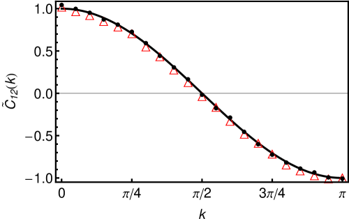
Figure 1: Fourier transform of given cross-correlation function $C_{12}$: solid curve is $\tilde{C}_{12}(k)$ entry of matrix (90); points correspond to numerically calculated cross-correlator of generated sequences $\{x_{1,2}^{C}(n)\}$ and triangles stand for numerically calculated cross-correlator of generated sequences $\{x_{1,2}^{H}(n)\}$.

7 Conclusion

In conclusion, let us summarize briefly the main results of the paper. Despite section 2 is introductory, it contains a few new results. We clarify the meaning of the filtering function $F(r)$ and show that it is the value of the cross-correlation function which describes correlations between the initial white noise and constructed correlated sequences. This function is determined up to the gauge factor containing an arbitrary odd function. There is no restriction on the parity of the filtering function.

In section 3 we present the matrix generalization of the method for a bunch of $N$ sequences. To construct $N$ cross-correlated sequences we start with $N$ independent uncorrelated white-noise random sequences $\{\xi_{i}(n)\}$. Similarly to the 1-sequence convolution method we built $N$ cross-correlated sequences $\{x_{i}(n)\}$ as a sum of convolutions of delta-correlated sequences $\{\xi_{j}(n)\}$ with filtering functions $F_{ij}(n)$. The set of these functions is obtained via the factorization of the Hermitian matrix $\tilde{\mathbf{C}}(k)$ into a product of the Fourier transforms of the generating function $\tilde{\mathbf{F}}(k)$ and its Hermitian transpose $\tilde{\mathbf{F}}^{\dagger}(k)$. Different decompositions of the correlation matrix are considered: spectral, Cholesky, LDL and Hermitian ansatz. Explicit expressions for some particular cases are presented. It was noticed that different decompositions of the correlation matrix provide the filtering matrix elements with essentially different analytical properties.

Statistical properties of the sequences constructed by the convolution method were examined. One-point probability distribution functions in the cases of weak and strong correlations were studied. The correlation function, integrated correlation function and the second integral of the correlation function (the variance of the sum of $L$ random variables) were found for asymmetric weak short-range correlations in the 1-sequence case. It was shown that the even part of the filtering function is responsible for generation of isotropic sequences. It will be interesting to study this phenomenon in the long-range correlation limit.

If the filtering function is smooth and a large number of summands contribute to equation (6), the distribution function $\rho_{X}(x)$ has the Gaussian or Lévy form.

An example of numerical construction of two correlated chains with a given correlation matrix was presented. Two different decompositions of the correlation matrix were used. It was shown that both of them give identical numerically reconstructed correlation functions (in spite of the difference of their analytical properties).

$$\xi(n)=\sum_{m=-N+1}^{N-1}\tilde{\xi}(k)\exp(ikn),\,\,k=k_{m}=\frac{2\pi}{N}m.$$ (104)

The Fourier coefficients are:

$$\Re\tilde{\xi}(k)=\frac{1}{N}\sum_{n=0}^{N}\xi(n)\cos kn,\,\,\Im\tilde{\xi}(k)=\frac{1}{N}\sum_{n=0}^{N}\xi(n)\sin kn.$$ (105)

Here symbols $\Re$ and $\Im$ stand for the real and the imaginary parts of a complex number. From equations (77), (105) and formulas $\sum_{n=0}^{N-1}\sin^{2}kn=(1-\delta_{k,0})N/2$,   $\sum_{n=0}^{N-1}\cos^{2}kn=(1+\delta_{k,0})N/2$, it follows that the random variables $\Re\tilde{\xi}(k)$ and $\Im\tilde{\xi}(k)$ are Gaussian distributed ones with variances $\sigma^{2}_{\Re\tilde{\xi}(k)}=(1+\delta_{k,0})/2N,\,\,\sigma^{2}_{\Im\tilde{\xi}(k)}=(1-\delta_{k,0})/2N$.

The values of $\Re\tilde{\xi}(k)$ and $\Im\tilde{\xi}(k)$ for negative $k$ (after generating $\Re\tilde{\xi}(k)$ and $\Im\tilde{\xi}(k)$ for $k>0$) have to be determined from relationships:

$$\Re\tilde{\xi}(-k)=\Re\tilde{\xi}(k),\,\,\,\Im\tilde{\xi}(-k)=-\Im\tilde{\xi}(k).$$ (106)

So, instead of generating a sequence $\{\xi(n)\}$ of uncorrelated random numbers and calculating then their Fourier transform coefficients, we can generate directly complex random numbers $\tilde{\xi}(k)=\Re\tilde{\xi}(k)+i\Im\tilde{\xi}(k)$.

To formulate the inverse statement let us consider the discrete Fourier transform for $\xi(n)$:

$$\xi(n)=a_{0}+\sum_{m=1}^{N-1}(a_{k}\cos kn+b_{k}\sin kn),\,\,k=k_{m}=\frac{2\pi}{N}m,$$ (107)

and suppose that the Fourier components $a_{k}$ and $b_{k}$ are independent and identically distributed variables with the variances $\sigma^{2}_{a_{k}}=\sigma^{2}_{b_{k}}=1/N$. We conclude that the random variables $\xi(n)$ are Gaussian distributed ones with equal variances $\sigma^{2}_{\xi(n)}=1$. This follows immediately from equation (77).

References

References

- [1] Mandelbrot B B, Wallis J R 1971 A Fast Fractional Gaussian Noise Generator Water Resour. Res. 7 543–53
- [2] R. F. Voss 1985 in: Fundamental Algorithms in Computer Graphics (Berlin: Springer) p 805
- [3] Shlesinger M F, Zaslavsky G M and Klafter J 1993 Strange kinetics Nature 363 31-7
- [4] Li W 1989 Spatial Spectra in Open Dynamical Systems Europhys. Let. 10 395-400
- [5] Usatenko O V, Apostolov S S, Mayzelis Z A and Melnik S S 2010 Random finite-valued dynamical systems: additive Markov chain approach (Cambridge: Cambridge Scientific Publisher) p 166
- [6] Czirok A, Mantegna R N, Havlin S and Stanley H E 1995 Correlations in Binary Sequences and a Generalized Zipf Analysis Phys. Rev. E 52 446–52
- [7] Makse H A, Havlin S, Schwartz M and Stanley H E 1996 Method for generating long range correlations for large systems Phys. Rev. E 53 5445–9
- [8] Carpena P, Bernaola-Galv́an P, Ivanov P Ch and Stanley H E 2002 Metal-insulator transition in chains with correlated disorder Nature 418 955-9
- [9] Carpena P, Bernaola-Galv́an P, Ivanov P Ch and Stanley H E 2003 Metal-insulator transition in chains with correlated disorder Nature 421 764
- [10] Hod S and Keshet U 2004 Phase transition in random walks with long-range correlations Phys. Rev. E 70, 015104(R)–7(R)
- [11] Narasimhan S L, Nathan J A and Murthy K P N 2005 Can coarse-graining introduce long-range correlations in a symbolic sequence? Europhys. Lett. 69 22–8
- [12] Narasimhan S L, Nathan J A, Krishna P S R and Murthy K P N 2006 A formalism for studying long-range correlations in many-alphabets sequences Physica A 367 252-60
- [13] Usatenko O V and Yampol’skii V A 2003 Binary N-step Markov chains and long-range correlated systems Phys. Rev. Lett. 90 110601-1 –4
- [14] Izrailev F M, Krokhin A A, Makarov N M and Usatenko O V 2007 Generation of correlated binary sequences from white noise Phys. Rev. E 76, 027701-1 – 4
- [15] Apostolov S S, Izrailev F M, Makarov N M, Mayzelis Z A, Melnyk S S and Usatenko O V 2008 The signum function method for the generation of correlated dichotomic chains J. Phys. A: Math. Theor. 41 175101-23
- [16] Izrailev F M, Krokhin A A and Makarov N M 2012 Anomalous localization in low-dimensional systems with correlated disorder Physics Reports 512 125-254
- [17] Rice S O 1944 Mathematical analysis of random noise Bell Syst. Tech. J. 23 282-332
- [18] Wax N 1953 Selected Papers on Noise and Stochastic Processes (New York, Dover) p 343
- [19] Saupe D 1988 The Science of Fractal Images (New York: Springer) p 312
- [20] West C S and O’Donnell K A 1995 Observations of backscattering enhancement from polaritons on a rough metal surface J. Opt. Soc. Am. A 12, 390 –7
- [21] Izrailev F M and Krokhin A A 1999 Localization and the Mobility Edge in One-Dimensional Potentials with Correlated Disorder Phys. Rev. Lett. 82 4062– 5
- [22] Izrailev F M and Makarov N M 2005 Anomalous transport in low-dimensional systems with correlated disorder J. Phys. A: Math. Gen. 38 10613–37
- [23] Cakir R, Grigolini P and Krokhin A A 2006 Dynamical origin of memory and renewal Phys. Rev. E 74 021108(1)–(6)
- [24] Romero A, Sancho J 1999 Generation of short and long range temporal correlated noises Journal of Computational Physics 156 1-11
- [25] Czirok A, Mantegna R N, Havlin S and Stanley H E 1995 Correlations in binary sequences and a generalized Zipf analysis Phys. Rev. E 52 446–52
- [26] Brockwell P J and Davis R A 2002 Introduction to Time Series and Forecasting, 2nd edition, (New York: Springer) p 437
- [27] Maystrenko A A, Melnik S S, Pritula G M and Usatenko O V Random linear antennas with managed radiation pattern, to be published in The Journal of Radiophysics and Electronics
- [28] Horn R A, Johnson Ch A 1990 Matrix Analysis (Cambridge: Cambridge University Press) p 575
- [29] Stewart G W 1996 Afternotes on numerical analysis, (Maryland: University of Maryland, College Park) p 200
- [30] Watkins D S 2010 Fundamentals of Matrix Computations (Wiley) p 664
- [31] Press W H, Teukolsky S A, Vetterling W T and Flannery B P 2007 Numerical Recipes, The Art of Scientific Computing (Cambridge: Cambridge University Press) p 1195
- [32] Deift P, Li C and Tomei C 1991 The bidiagonal singular value decomposition and Hamiltonian mechanics SIAM J. Numer. Anal. 18 1463–516
- [33] Hernandez-Herrejon J C, Izrailev F M and Tessieri L 2010 Electronic states and transport properties in the Kronig-Penney model with correlated compositional and structural disorder Physica E 42 2203–10
- [34] Usatenko O V, Yampol’skii V A, Kechedzhy K E and Mel’nyk S S 2003 Symbolic stochastic dynamical systems viewed as binary N-step Markov chains Phys. Rev. E 68 061107(1)–(14)
- [35] Apostolov S S, Mayzelis Z A, Mel’nyk S S, Usatenko O V and Yampol’skii V A 2007 Isotropy Properties of the Multi-Step Markov Symbolic Sequences Physica A 376 165–72