Generating Finite Dimensional Integrable Nonlinear Dynamical Systems^∗

Abstract

In this article, we present a brief overview of some of the recent progress made in identifying and generating finite dimensional integrable nonlinear dynamical systems, exhibiting interesting oscillatory and other solution properties, including quantum aspects. Particularly we concentrate on Lienard type nonlinear oscillators and their generalizations and coupled versions. Specific systems include Mathews-Lakshmanan oscillators, modified Emden equations, isochronous oscillators and generalizations. Nonstandard Lagrangian and Hamiltonian formulations of some of these systems are also briefly touched upon. Nonlocal transformations and linearization aspects are also discussed.

1 Introduction

Dynamical systems with finite degress of freedom/finite dimensions, whose underlying evolution equations are solvable in terms of analytic functions of elementary and transcendental types, are of extreme importance in physical, enginearing and biological sciencesGuc:1983 ; Tab:1989 ; Nayfeh:95 ; Wig:2003 ; Lakshmanan:03 . Particularly, systems exhibiting periodic oscillations of different types have considerable applicationsLakshmanan:03 ; Calogero:08 . Starting from the linear harmonic oscillator equation,

$$\ddot{x}+\omega_{0}^{2}x=0\;\;(^{.}=\frac{d}{dt}),$$ (1)

with suitable initial conditions, say $x(0)=A$, $\dot{x}(0)=0$, which is solvable in terms of the periodic function

$$x(t)=A\cos\omega_{0}t,$$ (2)

one can identify increasing number of autonomous and nonautonomous linear/nonlinear differential equations of different orders, nonlinearity and dimensions which are solvable in terms of suitable functions. Identifying such systems and understanding their solution properties of the underlying dynamical systems and developing new applications in the classical, semiclassical and quantum regimes are of fundamental significance. In this paper, we will be concerned with a class of such nonlinear integrable dynamical systems and their properties.

Consider the cubic undamped, free anharmonic oscillator described by the second order nonlinear ordinary differential equation (ODE),

$$\ddot{x}+\omega_{0}^{2}x+\lambda x^{3}=0\;\;(^{.}=\frac{d}{dt}),$$ (3)

with the initial conditions $x(0)=A$, $\dot{x}(0)=0$. The corresponding solution to the initial value problem is

$$x(t)=Acn(\Omega t,k),$$ (4)

where the frequency of oscillation as a function of the amplitude $A$ is

$$\Omega=\sqrt{\omega_{o}^{2}+\lambda A^{2}},$$ (5)

and the modulus square of the Jacobian elliptic function is

$$k^{2}=\frac{\lambda A^{2}}{2(\omega_{0}^{2}+\lambda A^{2})}.$$ (6)

Note that the frequency now depends on the amplitude or initial condition, which is a characteristic feature of typical nonlinear oscillators. In fact this dependence can become highly sensitive when suitable additional external force, nonlinearity, damping, etc. are added, leading to bifurcations and chaos Nayfeh:95 ; Lakshmanan:03 . A typical example is the Duffing oscillatorGuc:1983 ; Tab:1989 ; Nayfeh:95 ; Wig:2003 ; Lakshmanan:03 $\ddot{x}+\alpha\dot{x}+\omega_{0}^{2}x+\lambda x^{3}=f\cos\omega t$.

Then, the question arises as to whether nonlinear system always admit elliptic or higher functions and whether amplitude dependence of frequency of oscillations is a fundemental property of such oscillators. In this paper we will demonstrate that a large class of interesting nonlinear dynamical systems admitting elementary periodic solutions with or without dependence on initial conditions exist, apart from systems solvable by more complicated functions, and show the possibility of amplitude independent frequency of oscillations (isochronous propertyCalogero:08 ) and other related properties in a large class of nonlinear systems.

Specifically, we will consider the following class of dynamical systems (the following naming is our personal choice for convenience):
(a) Lienard type I:

$$\ddot{x}+f(x)\dot{x}^{2}+g(x)=0$$ (7)

(b) Lienard type II:

$$\ddot{x}+h(x)\dot{x}+g(x)=0$$ (8)

(c) Lienard type III:

$$\ddot{x}+f(x)\dot{x}^{2}+h(x)\dot{x}+g(x)=0$$ (9)

(d) Lienard type IV:

$$\ddot{x}+f(x,t)\dot{x}^{2}+h(x,t)\dot{x}+g(x,t)=0$$ (10)

(e) Coupled versions of the above Liénard type of dynamical systems:

$$\ddot{x}+f_{1}(x,y,t)\dot{x}^{2}+f_{2}(x,y,t)\dot{y}^{2}+f_{3}(x,y,t)\dot{x}\dot{y}$$

$$\qquad\qquad\qquad\qquad+h_{1}(x,y,t)\dot{x}+h_{2}(x,y,t)\dot{y}+g_{1}(x,y,t)=0$$

$$\ddot{y}+f_{4}(x,y,t)\dot{x}^{2}+f_{5}(x,y,t)\dot{y}^{2}+f_{6}(x,y,t)\dot{x}\dot{y}$$

$$\qquad\qquad\qquad\qquad+h_{3}(x,y,t)\dot{x}+h_{4}(x,y,t)\dot{y}+g_{2}(x,y,t)=0.$$ (11)

Here $f,g,h$, etc. are arbitrary functions in the indicated variables. Considering Liénard type I equation (7), one can identify an interesting class of nonlinear oscillators with velocity dependent or position dependent mass Hamiltonians of the form

$$H=\frac{1}{2}F(x)p^{2}+V(x),$$ (12)

having very interesting classical properties and quantum spectrum (see Sec. 2 for more details). 3-dimensional and N-dimensional generalizations corresponding to motion of dynamical systems on 3 and N dimensional spheres can be identified. Underlying Lie point symmetries of (7) can be classified as linearizable and integrable ones.

On the other hand system (8), though in general nonintegrable, can admit integrable dynamical systems under certain conditions. In particular, it can admit a class of nonstandard type Hamiltonian systems of the form

$$H=\frac{1}{2}F(p)x^{2}+U(p),$$ (13)

and generalizations (see Sec. 3 for further details). Of particular interest here is the modified Emden equation (MEE), which is of PT symmetric type and can be quantized in momentum space. N-dimensional generalizations of the above type of systems can also be identified. Finally we will consider some of the integrable versions of Eqs. (9)-(1) also in this paper.

The plan of the paper is as follows. In Sec. 2, we discuss Liénard type nonlinear oscillators (7) with quadratic velocity terms. In particular, we discuss Mathews-Lakshmanan oscillators and their generalizations and discuss their classical and quantum properties. In Sec. 3, we analyse the Liénard type oscillators (8) with linear velocity terms. Special attention is given to PT symmetric modified Emden equation (MEE) and generalizations and discuss the associated nonstandard Lagrangian and Hamiltonian formulations. Quantum aspects of the systems are also discussed. Higher dimensional integrable generalizations of MEEs are discussed in Sec. 4, while integrable Liénard type systems of the types III-IV are briefly discussed in Sec. 5, including infinite hierarchies. In Sec. 6, we briefly discuss other interesting systems including Painlevé and Gambier equations and present a brief outline of further challenges.

2 Liénard Type I systems: Mathews-Lakshmanan oscillators and generalization

Consider the dynamical equation

$$\ddot{x}+f(x)\dot{x}^{2}+g(x)=0.$$ (14)

Multiplying by an integrating factor $\dot{x}e^{2\int f(x)dx}$, one can obtain after one integrationMurphy:69

$$\dot{x}^{2}e^{2\int f(x)dx}+2\int g(x)e^{2\int f(x)dx}=I,$$ (15)

where $I$ is an integral of motion. In general this leads to velocity dependentMathews:74 or position dependent mass bend:98 Hamiltonian systems, depending on the forms of the functions $f(x)$ and $g(x)$:

$$H(x)=F(x)\frac{p^{2}}{2}+V(x),$$ (16)

where $p(x)$ is the canonically conjugate momentum, while $F(x)$ and $V(x)$ are functions related to $f(x)$ and $g(x)$.

2.1 Mathews-Lakshmanan (ML) oscillators

One of the most interesting examples is the case

$$f(x)=\frac{\lambda x}{(1-\lambda x^{2})},\;g(x)=\frac{\omega_{0}^{2}x}{(1-\lambda x^{2})},$$ (17)

where $\lambda$ and $\omega_{0}$ are constant parameters. Note that in the above, when $\lambda>0$, the range of displacement is restricted as $-1/\sqrt{\lambda}<x<1/\sqrt{\lambda}$, while for $\lambda<0$, there is no such restriction. The resulting system (14) is the Mathews-Lakshmanan oscillatorMathews:74 equation,

$$\ddot{x}+\frac{\lambda x}{(1-\lambda x^{2})}\dot{x}^{2}+\frac{\omega_{0}^{2}x}{(1-\lambda x^{2})}=0,$$ (18)

leading to the nonpolynomial Hamiltonian/Lagrangian

$$H=\frac{1}{2}\bigg{[}p^{2}(1-\lambda x^{2})+\frac{\omega_{0}^{2}x^{2}}{(1-\lambda x^{2})}\bigg{]},\;\;\;\;\;\;L=\frac{1}{2}\bigg{[}\frac{\dot{x}^{2}-\omega_{0}^{2}x^{2}}{(1-\lambda x^{2})}\bigg{]},$$ (19)

where

$$p=\frac{\dot{x}}{(1-\lambda x^{2})}.$$ (20)

The ML oscillator equation (18) may be considered as the zero-dimensional version of a scalar nonpolynomial field equationDelbourgo or as a velocity dependent potential oscillator. It can also be considered as an oscillator with a position dependent effective massKoc . The nonpolynomial oscillator system (18) exihibits simple harmonic periodic solutions but with amplitude dependent frequency,

$$x(t)=A\cos(\Omega t+\delta),\qquad\Omega=\frac{\omega_{0}}{\sqrt{1-\lambda A^{2}}}.$$ (21)

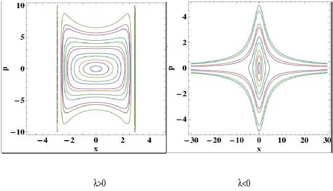
Figure 1: The phase plane structure of Mathews-Lakshmanan oscillator (18) (left) $\lambda>0$ and (right) $\lambda<0$.

The phase plane structure for the cases $\lambda>0$ and $\lambda<0$ are shown in Fig. 1.

It is interesting to note that the system (18) is linearizable under the nonlocal transformationGladwin Pradeep:09a

$$U=\frac{x}{\sqrt{1-\lambda x^{2}}},\;\;d\tau=\frac{1}{(1-\lambda x^{2})}dt,$$ (22)

so that

$$\frac{d^{2}U}{d\tau^{2}}+\omega_{0}^{2}U=0.$$ (23)

Solving (23) and using (22), one can indeed recover back the solution (21).

The quantum version of (19) is also exactly solvableMathews:75 . Symmetrizing the classical Hamiltonian in the quantum case as

$$H_{q}=\frac{1}{2}\bigg{[}\frac{1}{2}\hat{p}^{2}(1-\lambda\hat{x}^{2})+\frac{1}{2}(1-\lambda\hat{x}^{2})\hat{p}^{2}+\frac{\omega_{0}^{2}\hat{x}^{2}}{(1-\lambda\hat{x}^{2})}\bigg{]},$$ (24)

(where hat stands for linear differential operators) the time-independent Schrödinger equation $H_{q}\psi=E\psi$ can be written as the linear eigen value problem

$$(1-\lambda x^{2})\frac{d^{2}\psi}{dx^{2}}-2\lambda x\frac{d\psi}{dx}+\bigg{[}\frac{2E}{\hbar^{2}}+\frac{\omega_{0}^{2}}{\lambda\hbar^{2}}-\lambda-\frac{\omega_{0}^{2}}{\lambda\hbar^{2}}(\frac{1}{(1-\lambda x^{2})}\bigg{]}\psi=0.$$ (25)

On solving (25), for appropriate boundary conditions, the energy spectrum and eigenfunctions turn out to be the following: (i) $\lambda>0$:

$$E_{n}=(n+\frac{1}{2})\hbar\omega_{0}+\frac{1}{2}\lambda\hbar^{2}(n^{2}+n+1),\;\;n=0,1,2,\ldots$$ (26)

and

$$\psi_{n}=\left\{\begin{array}[]{cc}N_{n}P_{n+\mu}^{-\mu}\bigg{(}\lambda^{1/2}x\bigg{)},\quad|x|<\lambda^{-1/2},nonumber\\ \qquad\qquad 0,\quad|x|>\lambda^{-1/2},\;\mu=\frac{\omega_{0}}{\lambda\hbar}.\end{array}\right.,$$ (27)

(ii) $\lambda<0$:
(a) Bound States:

$$E_{n}=(n+\frac{1}{2})\hbar\omega_{0}-\frac{1}{2}|\lambda|\hbar^{2}(n^{2}+n+1),\;\;n=0,1,2,\ldots,N.$$ (28)

and

$$\psi_{n}=\left\{\begin{array}[]{cc}N_{n}Q_{\mu-(n+1)}^{\mu}\bigg{(}|\lambda|^{1/2}x\bigg{)},\quad|x|<|\lambda|^{1/2},\\ \qquad\quad 0,\quad|x|>|\lambda|^{1/2}.\end{array}\right.,$$

(b) Scattering states:

$$\psi(x)=NP_{-\frac{1}{2}+ip}^{-\mu}\bigg{(}\lambda^{1/2}x\bigg{)}\Theta\bigg{(}|\lambda|^{1/2}x-1\bigg{)}.$$ (29)

In the above $P_{\mu}^{\gamma}(x)$and $Q_{\mu}^{\gamma}(x)$ are associated Legendre functionsMathews:75 and $\Theta$ is the Heaviside step function.

2.2 Three-dimensional and N-dimensional generalizations:

A three dimensional generalization of the ML oscillator (18) corresponds to the HamiltonianLakshmanan:75

$$H=\frac{1}{2}\bigg{[}\vec{p}^{2}-\lambda(\vec{p}.\vec{q})^{2}+\frac{\omega_{0}^{2}\vec{q}^{2}}{(1-\lambda\vec{q}^{2})}\bigg{]},\;\;\vec{q}=(q_{1},q_{2},q_{3}).$$ (30)

It is the zero-dimensional isoscalar version of the SU(2)$\otimes$SU(2) chiral model in the Gasiorowicz-Geffen coordinatesLakshmanan:75 . The associated canonical equations of motion can be rewritten in the form

$$\ddot{q}_{i}+\left[\frac{\lambda(\vec{q}.\ddot{\vec{q}})}{(1-\lambda\vec{q}^{2})}+\frac{\lambda\dot{\vec{q}}^{2}}{(1-\lambda\vec{q}^{2})}+\frac{\lambda^{2}(\vec{q}.\dot{\vec{q}})^{2}}{(1-\lambda\vec{q}^{2})^{2}}+\frac{\omega_{0}^{2}}{(1-\lambda\vec{q})^{2}}\right]q_{i}=0.$$ (31)

In spherical polar coordinates

$$\vec{q}=(q\sin\theta\cos\phi,q\sin\theta\sin\phi,q\cos\theta),$$ (32)

Eq. (31) can be separated out as

$$\dot{\phi}=\frac{C_{1}}{q^{2}\sin^{2}\theta},\;\;\quad q^{4}\dot{\theta}^{2}=C_{2}^{2}-\frac{C_{1}^{2}}{\sin^{2}\theta},$$

$$\ddot{q}+\frac{\lambda q\dot{q}^{2}}{1-\lambda q^{2}}+\frac{\omega_{0}^{2}q}{1-\lambda q^{2}}=\frac{C_{2}^{2}(1-\lambda q^{2})}{q^{3}},$$ (33)

where $C_{1}$ and $C_{2}$ are constants. On integration one can write down the solution as

$$q(t)=A\left[1-\beta\sin^{2}\Omega t\right]^{\frac{1}{2}},\quad\Omega^{2}=\frac{\omega_{0}^{2}}{(1-\lambda A^{2})}+\frac{\lambda C_{2}^{2}}{A^{2}}$$ (34)

where $\beta=1-\frac{1}{\lambda A^{2}}\bigg{(}1-\lambda A^{2}-\frac{\omega_{0}^{2}-\lambda^{2}C_{2}}{\Omega^{2}}\bigg{)}$ and $A$ is the integration constant.

In fact the above system can be interpretedhiggs as an isotropic oscillator moving on a 3-sphere, $q_{1}^{2}+q_{2}^{2}+q_{3}^{2}=\sqrt{\lambda}$.

The associated quantum Hamiltonian can be symmetrized in the form

$$H_{q}=\frac{1}{2}\vec{\hat{p}}^{2}-\lambda(\vec{\hat{p}}.\vec{\hat{q}})(\vec{\hat{q}}.\vec{\hat{p}})+\frac{\omega_{0}^{2}\vec{\hat{q}}^{2}}{1-\lambda\vec{\hat{q}}^{2}}.$$ (35)

From the Lie symmetries associated with system (31), one can identify the following symmetry generators and Lie algebra for the quantum system (35):

$$J_{i}=\epsilon_{ijk}(q_{j}p_{k}-p_{j}q_{k}),\;\;\;i,j,k=1,2,3,$$

$$F_{i}=\frac{1}{2}\left[(1-\lambda\vec{q}^{2})^{\frac{1}{2}}p_{i}+p_{i}(1-\lambda\vec{q}^{2})^{\frac{1}{2}}\right],$$ (36)

so that a nonlinear algebra can be realized.

$$[J_{i},J_{j}]=i\epsilon_{ijk}J_{k},\,\,\,\,\,[F_{i},F_{j}]=i\lambda\epsilon_{ijk}J_{k},\,\,\,[J_{i},F_{j}]=\frac{i}{\lambda}\epsilon_{ijk}F_{k},$$

$$[F_{i},q_{j}]=-\frac{1}{\lambda}\sqrt{1-\lambda q^{2}}\delta_{ij}.$$ (37)

Depending on whether $\lambda>0$ or $\lambda<0$, one has an SO(4) or SO(3,1) algebra, respectively. The problem can be generalized to N-dimensionas and the associated nonlinear algebra can be written down as was done by Higgshiggs and LeemonLeemon:79 . Such algebras in fact are the precursors to the study of quantum groups13 .

The three dimensional quandum problem itself can be solved completelyLakshmanan:75 namely $H_{q}\psi_{nlm}=E_{n}\psi_{nlm}$, in spherical polar coordinates. The eigenvalues and eigenfunctions turn out to be

$$E_{n}=(n+\frac{3}{2}\hbar\omega_{0})+\frac{1}{2}\lambda\hbar^{2}(n^{2}+3n),(n=2n_{i}+l),\;i=1,2,\ldots$$

$$\psi_{n}=A(1-\lambda q^{2})^{\frac{1}{2}}q^{\mu-1}F(\frac{1}{2}\mu+\frac{1}{2}\nu+\frac{1}{2}p,-n;\mu+\frac{1}{2},\lambda q^{2})$$

$$\hskip 56.9055pt\times Y_{lm}(\theta,\phi),\quad 0\leq q<\lambda^{-\frac{1}{2}}$$ (38)

where $Y_{lm}$ are the spherical harmonics and $F(\alpha,\beta,\gamma;x)$ is the hypergeometric function. For certain class of N-dimensional version of the above systems corresponding to an isotropic oscillator moving on an N-sphere, one can again solve the quantum machanical eigenvalue problem. For a complete solution, see for examplehiggs . These problems continue to evoke considerable interest in the literature in their classical and quantum versions for their oscillatory properties, energy level spectra, eigenfunctions, construction of creation and annihilation operators, coherent states and generalizations leading to bifurcations and chaos15 ; Carinena:04 ; Carinena:07 ; Tewari:13 ; Bhuneshwari:12 ; Bagchi:13 ; Cruz:13 .

A particularly interesting completely integrable N-degrees of freedom system introduced by Carinena et al.Carinena:04 is

$$H=\frac{1}{2}\left[\sum p_{i}^{2}+\lambda(\sum_{i=1}^{N}q_{i}p_{i})^{2}\right]+\frac{\alpha^{2}}{2}\left(\frac{q^{2}}{1-\lambda q^{2}}\right),\,\,q^{2}=\sum_{i=1}^{N}q_{i}^{2}.$$ (39)

The higher dimensional equation (39) is superintegrable with $2N-1$ quadratic constants of motion.

Finally the case

$$f(x)=\frac{\lambda x}{(1+\lambda x^{2})},\;\;\;g(x)=\frac{\omega_{0}^{2}}{(1+\lambda x^{2})}$$ (40)

in Eq. (14) is also of considerable interest which corresponds to the motion of a particle on a rotating parabola and the corresponding damped and forced version exhibits a rich variety of bifurcations and chaos phenomena, see for more details ref.15 ; Bagchi:13 .

2.3 Lie point symmetries and isochronous oscillators

It is of interest to consider the Lie point symmetriesTewari:13 associated with Eq. (7). It can be shown that it admits eight, three, two and one parameter symmetries. In particular, the case corresponding to eight parameter symmetries is linearizable under coordinate transformations, in confirmty with the general theory of Lie on group classification of ODEs. This case corresponds to the choice

$$g(x)=e^{-\int f(x)dx}\left[g_{1}\int dxe^{\int f(x)dx}+g_{2}\right],$$ (41)

where $g_{1}$ and $g_{2}$ are arbitrary constants and $f(x)$ is any given function in Eq. (14). In this case, one can consider a transformation of the form

$$X(x)=\frac{g_{1}}{\omega_{0}^{2}}\left[\int e^{\int f(x)dx}dx+\frac{g_{2}}{\omega_{0}^{2}}\right]$$ (42)

which linearizes equation (7) to the linear harmonic oscillator form (1). Consequently the solution of (7) will be periodic with period $T=\frac{2\pi}{\omega_{0}}$, which is the same as that of the linear harmonic oscillator (Note that the solution may be regular or singular depending on the form of $f(x)$).

A typical example is the perturbed Morse type oscillator

$$\ddot{x}+\lambda\dot{x}^{2}+\frac{\omega_{0}^{2}}{\lambda}(1-e^{-\lambda x})=0$$ (43)

corresponding to the Hamiltonian

$$H=\frac{1}{2\lambda^{2}}e^{-2\lambda x}p^{2}+\frac{1}{2}\omega_{0}^{2}(1-e^{-\lambda x}),$$ (44)

where the canonically conjugate momentum $p=\lambda^{2}e^{2\lambda x}\dot{x}$. The isochronos solution of (43) is then given by

$$x(t)=\frac{1}{\lambda}\ln[1-\lambda A\sin(\omega_{0}t+\delta)],\;\;0\leq A<\frac{1}{\lambda}.$$ (45)

The system can also be quantized as in the case of ML oscillator. One can find the general form of integrable systems of (7) with three and two parameter symmetries whose integrals can be constructed from the symmetries. However, remarkably the ML oscillator possesses only one Lie point symmetry. Yet it is integrable, the reason being that it possesses the so called $\lambda$-symmetry which is essentially of nonlocal typeBhuneshwari:12 .

3 Liénard Type II system: Modified Emden Equation and Generalizations - Nonlocal Transformations

The standard Liénard system

$$\ddot{x}+h(x)\dot{x}+g(x)=0$$ (46)

can also be classified group theoreticallyPandey:09 . It possesses Lie point symmetries which can be eight, three, two or one. The conditions for eight parameter symmetries to exist are

$$h_{xx}=0,\qquad 3g_{xx}-2hh_{x}=0,$$ (47)

implying

$$h(x)=ax+b,\qquad g(x)=\frac{2a}{3}(\frac{a}{6}x^{3}+\frac{b}{2}x^{2}+cx+d),$$ (48)

where $a,b,c$ and $d$ are constant parameters. In a similar way one can classify all the forms of (46) possessing three and two point symmetries and their integrability can be established. The full equation (46) for arbitrary form of $h(x)$ and $g(x)$ possesses at least one point symmetry whose integrability depends on the specific forms of $f(x)$ and $g(x)$.

3.1 The Modified Emden Equation (MEE)

An interesting case belonging to the family of Liénard type II equation possessing eight parameter Lie point symmetries satisfying the criteria (47) or (48) is the MEEmah:1985 ; Chandrasekar:05 ,

$$\ddot{x}+kx\dot{x}+\frac{k^{2}}{9}x^{3}+\omega_{0}^{2}x=0.$$ (49)

Eq. (50) is linearizable under the nonlocal transformation

$$U(t)=x(t)e^{k\int xdt}$$ (50)

so that $\ddot{U}+\omega_{0}^{2}U=0$, $U=A\sin(\omega_{0}t+\delta)$, and

$$\dot{x}-\frac{\dot{U}}{U}x+kx^{2}=0.$$ (51)

Consequently, solving the Riccati equation, we obtain the general solution as

$$x(t)=\frac{A\sin(\omega_{0}t+\delta)}{1-\frac{kA}{3\omega_{0}}\cos(\omega_{0}t+\delta)},\quad 0\leq A<\frac{3\omega_{0}}{k}.$$ (52)

Note that the frequency is independent of the amplitude of oscillations or the solution (52) is isochronousCalogero:08 . The integrability of system (50) can be proved by finding two explicit time dependent integralsChandrasekar:05 , from which one time independent integral can be identified. Consequently a nonstandard Hamiltonian and Lagrangian description can be developed for (50) with the forms

$$L=\frac{27\lambda_{1}^{3}}{2k^{2}}\bigg{(}\frac{1}{k\dot{x}+\frac{k^{2}}{3}x^{2}+3\lambda_{1}}\bigg{)}+\frac{3\lambda_{1}}{2k}\dot{x}-\frac{9\lambda_{1}^{2}}{2k^{2}},$$ (53a)

$$p=\left(\frac{-27\omega_{0}^{6}}{2k(k\dot{x}+\frac{k^{2}}{3}x^{2}+3\omega_{0}^{2})^{2}}\right),$$ (53b)

$$H=\frac{1}{2}F(p)x^{2}+U(p),\quad F(p)=\omega_{0}^{2}\left(1-\frac{2k}{3\omega_{0}^{2}}p\right),$$ (53c)

$$U(p)=\frac{9\omega_{0}^{4}}{2k^{2}}\left(\sqrt{1-\frac{2k}{3\omega_{0}}p}-1\right)^{2},$$ (53d)

The isochronous time series and the phase space structure is shown in Fig. 2. Note that the trajectries are bounded in the upper half $(x,p)$ plane by the condition $p\leq\frac{3\omega_{0}^{2}}{2k}$, beyond which the trajectories become complex.

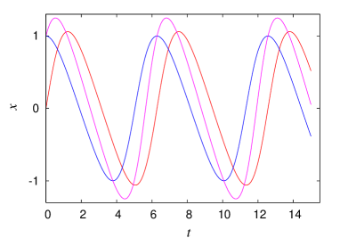
Figure 2: (left) Time series and (right) $(x-p)$ phase plane structure of MEE.

It is also of interest to compare the Hamiltonian structure of the Liénard type II MEE given by (53c) with the structure (16) of the quadratic Liénard type I equation, where the role of $x$ and $p$ are interchanged. The quadratic structure in $x$ of the Hamiltonian (53c) allows one to quantize Chithika Ruby:12 the system exactly, now not in coordinate space but in momentum space. Before presenting the results briefly, we also note the fact that the MEE (50) is invariant under the combined reversible transformation $x\rightarrow-x$ and $t\rightarrow-t$ so that (50) and (53c) are PT symmetric systems but now for real dynamical variables. Note that the standard PT symmetric systems are PT invariant for complex dynamical variablesChithika Ruby:12 ; bender_r . It appears that in this context system (50) is unique.

To quantize the system (53c), one can rewrite the classical Hamiltonian in the position dependent mass form

$$H(x,p)=\frac{1}{2}\frac{x^{2}}{m(p)}+U(p),$$ (54)

where

$$m(p)=\omega^{-2}\;\left(1-\frac{2k}{3\omega^{2}}p\right)^{-1},\quad U(p)=\frac{9\omega^{4}}{2k^{2}}\left(\sqrt{1-\frac{2k}{3\omega^{2}}p}-1\right)^{2},\omega=\omega_{0}.$$

We can now quantize the system in the momentum space using the so called von Roos orderingvon and with the operator replacement ${\displaystyle\hat{x}=i\hbar\frac{d}{dp}}$ in the time independent Schrödinger equation,

$$H(\hat{x},i\hbar\frac{d}{dp})\Psi(x,p)=E\Psi(p),$$ (55)

along with the boundary conditions $\Psi(-\infty)=\Psi\left(\frac{3\omega^{2}}{2k}\right)=0$. For admissible wavefunctions, one can show that the appropriate Hamiltonian for the present problem is

$$H(\hat{x},\hat{p})=\frac{1}{2}\left[m^{-1/4}(\hat{p})\hat{x}m^{-1/2}(\hat{p})\hat{x}m^{-1/4}(\hat{p})\right]+U(\hat{p}),$$ (56)

so that the Schrödinger equation becomes

$$-\frac{\hbar^{2}\omega^{2}}{2}\left(1-\frac{2k}{3\omega^{2}}p\right)\Phi^{\prime\prime}-\frac{\hbar^{2}k^{2}}{24\omega^{2}\left(1-\frac{2k}{3\omega^{2}}p\right)}\Phi+\frac{9\omega^{4}}{2k^{2}}\left(\sqrt{1-\frac{2k}{3\omega^{2}}p}-1\right)^{2}\Phi=E\Phi,$$

where $\left({}^{\prime}=\frac{d}{dp}\right)$. Note that the Hamiltonian (56) is non-hermitian and nonsymmetric associated with its PT symmetric nature. There are two sectors of solutions as given below.

(i) Case 1: The sector $-\infty<p\leq\frac{3\omega^{2}}{2k}$:
  The PT invariant solution is

$$\Phi_{n}(p)=\left\{\begin{array}[]{cc}\tilde{N}_{n}\left(1-\frac{2k}{3\omega^{2}}p\right)^{1/4}\exp{\left(-\frac{9\omega^{3}}{2\;\hbar\;k^{2}}\left(1-\frac{2k}{3\omega^{2}}p-2\sqrt{1-\frac{2k}{3\omega^{2}}p}\right)\right)}\\ \hskip 85.35826pt\times H_{n}\left[\frac{3\omega^{3/2}}{\sqrt{\hbar}\;k}\left(\sqrt{1-\frac{2k}{3\omega^{2}}p}-1\right)\right],-\infty<p\leq\frac{3\omega^{2}}{2k},\\ 0,\quad p\geq\frac{3\omega^{2}}{2k},\end{array}\right.$$

with the associated eigenvalue spectrum as just that of the linear harmonic oscillator,

$$E_{n} = (n+\frac{1}{2})\;\hbar\;\omega,\qquad\quad n=0,1,2,....$$ (57)

In the above $H_{n}$’s are the Hermite polynomials and $N_{n}$ is the normalization constant.

(ii) Case 2: The sector $p>\frac{2\omega}{2k}$:

$$\Phi_{n}(p)=\left\{\begin{array}[]{cc}\tilde{\cal{N}}_{n}\left(\frac{2k}{3\omega^{2}}p-1\right)^{1/4}\exp{\left(-\frac{9\omega^{3}}{2\;\hbar\;k^{2}}\left(\frac{2k}{3\omega^{2}}p-1+i\;2\sqrt{\frac{2k}{3\omega^{2}}p-1}\right)\right)}\\ \hskip 85.35826pt\times H_{n}\left[\frac{3\omega^{3/2}}{\sqrt{\hbar}\;k}\left(\sqrt{\frac{2k}{3\omega^{2}}p-1}+i\right)\right],\quad p\geq\frac{3\omega^{2}}{2k},\\ \qquad\quad 0,\quad-\infty<p\leq\frac{3\omega^{2}}{2k},\end{array}\right.,$$

($\tilde{\cal{N}}_{n}$ is the normalization constant) with energy eigenvalues without a lower bound

$$E_{n}=-(n+\frac{1}{2})\hbar\omega,\quad n=0,1,2,3,....$$ (58)

Note that the eigenfunctions are no longer PT symmetric, even though the Hamiltonian (56) is, leading to a negative energy spectrum which is unbounded below, a property shared by other complex valued PT symmetric potentialsbender_r .

Thus one finds the above MEE and its quantized version turns out to be possessing unusual structures. Higher dimensional generalization of this system is indeed possible both at the classical and quantum levels, which will be presented elsewhere.

It is not only the specific form (50) of MEE which is integrable. Even the generalized versionfeix:1997 ; Chandrasekar:07 ; Gladwin Pradeep:09a

$$\ddot{x}+\alpha x\dot{x}+\beta x^{3}+\omega_{0}^{2}x=0,$$ (59)

where $\alpha$ and $\beta$ are arbitrary parameters, is completely integrableChandrasekar:07 and time independent integrals of motion and solutions upto quadrature can be written down Chandrasekar:07 . However, in this case the structure of the integrals and solutions are more complicated. For details see Chandrasekar et al.Chandrasekar:07 . A simple way to look at the integrability of (59) is that it is linearizable under the nonlocal transformation

$$y=\frac{x^{2}}{2}+\frac{\omega_{0}^{2}}{\lambda},\qquad d\tau=xdt$$ (60)

so that one obtains damped linear harmonic oscillator equation,

$$\frac{d^{2}y}{d\tau^{2}}+\alpha\frac{dy}{d\tau}+\lambda y=0.$$ (61)

In fact one can generalize this result by considering a more general nonlocal transformation

$$y=\int f(x)dx,\qquad d\tau=\frac{f(x)}{g(x)}dt,$$ (62)

so that the general class of Liénard type equation III

$$\ddot{x}+\frac{g^{\prime}(x)}{g(x)}\dot{x}^{2}+\alpha\frac{f(x)}{g(x)}\dot{x}+\lambda\frac{f(x)}{g(x)^{2}}\int f(x)dx=0$$ (63)

itself gets linearized to (61). This allows one to associate a nonstandard Lagrangian and Hamiltonian description to (63) as shown in Gladwin Pradeep et al.Gladwin Pradeep:09a . For further discussion on nonstandard Lagrangian/Hamiltonian formulation, see for example refs.Musielak:08 ; Cie:10

4 Higher dimensional coupled integrable versions of MEE

An interesting two dimensional generalization of MEE given by (50) can be identifiedGladwin Pradeep:09b as

$$\ddot{x}=-2(k_{1}x+k_{2}y)\dot{x}-(k_{1}\dot{x}+k_{2}\dot{y})x-(k_{1}x+k_{2}y)^{2}x-\lambda_{1}x,$$

$$\ddot{y}=-2(k_{1}x+k_{2}y)\dot{y}-(k_{1}\dot{x}+k_{2}\dot{y})y-(k_{1}x+k_{2}y)^{2}y-\lambda_{2}y.$$ (64)

Eq. (64) can be linearized under the nonlocal transformation

$$U=xe^{\int(k_{1}x+k_{2}y)dt},\;\;V=ye^{\int(k_{1}x+k_{2}y)dt}.$$ (65)

so that

$$\ddot{U}+\lambda_{1}U=0,\;\;\ddot{V}+\lambda_{2}V=0.$$ (66)

From (65), one can also identify a set of coupled Riccati equations,

$$\dot{x}=\frac{\dot{U}}{U}x-k_{1}x^{2}-k_{2}xy,\quad\dot{y}=\frac{\dot{V}}{V}y-k_{1}xy-k_{2}y^{2}.$$ (67)

Solving the system (67) one can obtain the explicit oscillatory solutions,

$$x(t)=\frac{A\sin(\omega_{1}t+\delta_{1})}{1-\frac{Ak_{1}}{\omega_{1}}\cos(\omega_{1}t+\delta_{1})-\frac{Bk_{2}}{\omega_{2}}\cos(\omega_{2}t+\delta_{2})},$$

$$y(t)=\frac{B\sin(\omega_{2}t+\delta_{2})}{1-\frac{Ak_{1}}{\omega_{1}}\cos(\omega_{1}t+\delta_{1})-\frac{Bk_{2}}{\omega_{2}}\cos(\omega_{2}t+\delta_{2})},\,\,$$

$$\hskip 199.16928pt\bigg{|}\frac{Ak_{1}}{\omega_{1}}+\frac{Bk_{2}}{\omega_{2}}\bigg{|}<1,$$

where $\omega_{j}=\sqrt{\lambda_{j}},\;j=1,2,\,\bigg{|}\frac{Ak_{1}}{\omega_{1}}+\frac{Bk_{2}}{\omega_{2}}\bigg{|}<1$. Note that the solution may be periodic or quasiperiodic depending on the value of the ratio $\omega_{1}/\omega_{2}$, that is whether it is rational or irrational. Typical solutions are plotted in Fig. 3.

Figure 3: (a) Quasi-periodic oscillations ($\omega_{1}=1$ and $\omega_{2}=\sqrt{2}$) (b) periodic oscillations ($\omega_{1}=1$ and $\omega_{2}=5$) of Eq. (64). Here (i) phase space plot (ii) Configuration space plot and (iii) Poincaré SOS.

The system (59) also admits four independent integrals, two of which are time independent and the remaining two are time dependent:

$$I_{1}=\frac{(\dot{x}+(k_{1}x+k_{2}y)x)^{2}+\lambda_{1}x^{2}}{\left[\frac{k_{1}}{\lambda_{1}}(\dot{x}+(k_{1}x+k_{2}y)x)+\frac{k_{2}}{\lambda_{2}}(\dot{y}+(k_{1}x+k_{2}y)y)+1\right]^{2}},$$ (68a)

$$I_{2}=\frac{(\dot{y}+(k_{1}x+k_{2}y)y)^{2}+\lambda_{2}y^{2}}{\left[\frac{k_{1}}{\lambda_{1}}(\dot{x}+(k_{1}x+k_{2}y)x)+\frac{k_{2}}{\lambda_{2}}(\dot{y}+(k_{1}x+k_{2}y)y)+1\right]^{2}},$$ (68b)

$$I_{3}=\left\{\begin{array}[]{ll}\tan^{-1}\left[\frac{\sqrt{\lambda_{1}}x}{\dot{x}+(k_{1}x+k_{2}y)x}\right]-\sqrt{\lambda_{1}}\,t,&\lambda_{1}>0\\ \frac{e^{2\sqrt{|\lambda_{1}|}t}(\dot{x}+(k_{1}x+k_{2}y)x-\sqrt{|\lambda_{1}|}x)}{\dot{x}+(k_{1}x+k_{2}y)x+\sqrt{|\lambda_{1}|}x},&\lambda_{1}<0,\end{array}\right.$$ (71)

and

$$I_{4}=\left\{\begin{array}[]{ll}\tan^{-1}\left[\frac{\sqrt{\lambda_{2}}y}{\dot{y}+(k_{1}x+k_{2}y)y}\right]-\sqrt{\lambda_{2}}\,t,&\lambda_{2}>0\\ \frac{e^{2\sqrt{|\lambda_{2}|}t}(\dot{y}+(k_{1}x+k_{2}y)x-\sqrt{|\lambda_{2}|}y)}{\dot{y}+(k_{1}x+k_{2}y)y+\sqrt{|\lambda_{2}|}y},&\lambda_{2}<0.\end{array}\right.$$ (74)

The system (59) does admit a singular Lagrangian for the case $\lambda_{1}=\lambda_{2}=\lambda$ as

$$L=\frac{1}{\left[k_{1}(\dot{x}+(k_{1}x+k_{2}y)x)+k_{2}(\dot{y}+(k_{1}x+k_{2}y)y)+\lambda\right]}.$$ (75)

The problem of constructing appropriate Lagrangian and Hamiltonian to (64) still remains an open problem. One can generalize the above results to a system of N-coupled MEEs,

$$\ddot{x}_{i}+2\sum_{j=1}^{N}k_{j}x_{j}\dot{x}_{i}+\sum_{j=1}^{N}k_{j}\dot{x}_{j}x_{i}+(\sum_{j=1}^{N}k_{j}x_{j})^{2}x_{i}+\lambda_{i}x_{i}=0,\;i=1,2,...,N,$$ (76)

and obtain the explicit periodic solutions. The associated 2N integrals turn out to be

$$I_{1i}=\frac{(\dot{x}_{i}+\sum_{j=1}^{N}(k_{j}x_{j})x_{i})^{2}+\lambda_{i}x_{i}^{2}}{\left[\sum_{j=1}^{N}\left[\frac{k_{j}}{\lambda_{j}}(\dot{x}_{j}+\sum_{n=1}^{N}(k_{n}x_{n})x_{j})\right]+1\right]^{2}},$$ (77)

$$I_{2i}=\tan^{-1}\left[\frac{\sqrt{\lambda_{i}}x_{i}}{\dot{x}_{i}+\sum_{j=1}^{N}(k_{j}x_{j})x_{i}}\right]-\sqrt{\lambda_{i}}t,\,\,\,\lambda_{i}>0,$$ (78)

We also note here that one can make appropriate contact-type transformations to (76) which maps them onto a system of N uncoupled harmonic oscillators.

4.1 Generalized nonlocal transformations and integrable N-coupled dynamical systems

Consider the set of uncoupled linear harmonic oscillators

$$\ddot{U}_{i}+\omega_{i}^{2}U_{i}=0,\;\;i=1,2,\ldots,N.$$ (79)

Under the nonlocal transformation

$$U_{i}=x_{i}e^{\int f_{i}(x_{1},x_{2},\ldots,x_{N})dt},$$ (80)

Eqs. (79) gets transformed toChandrasekar:12

$$\ddot{x}_{i}+\sum_{j=1}^{N}f_{i}^{(j)}(\overline{x})x_{i}\dot{x}_{j}+f_{i}(\overline{x})\dot{x}_{i}+f_{i}^{2}(\overline{x})x_{i}+\omega_{i}^{2}x_{i}=0,\,\,i=1,2,\ldots,N,$$ (81)

where $f_{i}^{(j)}=\frac{df_{i}}{dx_{j}}$ and $\overline{x}=(x_{1},x_{2},\ldots,x_{N})$. Then using the Riccati connection, we can obtain the set of first order ODEs,

$$\dot{x}_{i}=\frac{\omega_{i}}{\tan(\omega_{i}t+\delta_{i})}x_{i}-f_{i}(x_{1},x_{2},\ldots,x_{N})x_{i},\quad i=1,2,\ldots N.$$ (82)

($\delta_{i}$’s : $N$-integration constants). For the special choice

$$f_{k}=f_{N}(\bar{x})=f(\bar{x})=f(x_{1},x_{2},\ldots x_{N}),\;k=1,2,\ldots,N-1,$$ (83)

$(N-1)$ integrals can be obtained from the relations

$$\frac{x_{k}}{x_{N}}=I_{k}\frac{\sin(\omega_{k}t+\delta_{k})}{\sin(\omega_{N}t+\delta_{N})}=h_{k}(t),\;\;k=1,2,\ldots,N-1$$ (84)

where $I_{k}$’s are the (N-1) independent integrals.

Then the problem (81) reduces to the problem of solving a single first order ODEChandrasekar:12 :

$$\dot{x}_{N}=\frac{\omega_{N}x_{N}}{\tan(\omega_{N}t+\delta_{N})}-f(\bar{h}(t),x_{N})x_{N}.$$ (85)

The associated integrals can be explicitly given as

$$I_{k}^{2} = \frac{(\omega_{k}^{2}x_{k}^{2}+(\dot{x}_{k}+f(\bar{x})x_{k})^{2})}{(\omega_{N}^{2}x_{N}^{2}+(\dot{x}_{N}+f(\bar{x})x_{N})^{2})},\;\;k=1,2,\ldots,N-1.$$ (86)

The remaining integral $I_{N}$ can be obtained by solving the Riccati equation (85) for appropriate forms of $f$. One can extend this procedure to analyse even nearby nonintegrable systemsChandrasekar:12 .

5 Singular and nonsingular isochronous Hamiltonian systems

In the following we briefly discuss the procedure to deduce singularsingular2 and nonsingular Hamiltonian systems associated with a class of isochronous systemsCalogero:07 ; Calogero:08a .

5.1 Singular isochronous Hamiltonian systems

Let us consider an $N$-dimensional system with a Hamiltonian of the formGladwin Pradeep:12c involving velocity dependent potentials,

$$\tilde{H}(\underline{p},\underline{q};\Omega) = \frac{1}{2}\left[\left\{\sum_{n=1}^{N}a_{n}p_{n}\left(\frac{\partial Q(\underline{q})}{\partial q_{n}}\right)^{-1}\right\}^{2}+\Omega^{2}Q(\underline{q})^{2}\right],$$ (87)

where $a_{n}$ and $\Omega$ are constants, $\underline{p}=(p_{1},p_{2},...,p_{N})$ and $\underline{q}=(q_{1},q_{2},...,q_{N})$ and $Q(\underline{q})$ is an arbitrary function of the canonical coordinates $q^{\prime}_{n}s,\,\,n=1,2,...N$. Hamiltonian (87) results in the following $2N$ coupled first order canonical equations of motion for the canonical coordinates $q_{n}$ and $p_{n}$,

$$\dot{q}_{n}=a_{n}\left[\frac{\partial Q(\underline{q})}{\partial q_{n}}\right]^{-1}H,\qquad n=1,2,\ldots,N$$ (88a)

$$\dot{p}_{n}=H\sum_{m=1}^{N}\left\{a_{m}p_{m}\left[\frac{\partial Q(\underline{q})}{\partial q_{m}}\right]^{-2}\left[\frac{\partial^{2}Q(\underline{q})}{\partial q_{m}\partial q_{n}}\right]\right\}-\Omega^{2}Q(q)\frac{\partial Q(\underline{q})}{\partial q_{n}}.$$ (88b)

The corresponding Newton’s equation of motion is obtained by differentiating (88a) with respect to $t$ and using (88b) for $\dot{p}_{n}$. It is given in the form

$$\frac{\partial Q(\underline{q})}{\partial q_{n}}\ddot{q}_{n}+\sum_{m=1}^{N}\bigg{(}\dot{q}_{n}\dot{q}_{m}\frac{\partial^{2}Q(\underline{q})}{\partial q_{n}q_{m}}\bigg{)}+\Omega^{2}a_{n}Q(\underline{q})=0,n=1,2,\ldots,N.$$ (89)

However, one can easily check that not all the coordinates $q_{i},\,\,i=1,2,\ldots,N$ are independent: there are $(N-1)$ holonomic constraints existing between themGladwin Pradeep:12c :

$$\int dq_{1}\frac{\partial Q}{\partial q_{1}}-\int dq_{j}\frac{\partial Q}{\partial q_{j}}=C_{j},\quad j=2,3,\ldots,N,$$ (90)

where $C_{j}$’s are constants. Equation (90) obviously constitutes a set of $(N-1)$ holonomic constraints on the coordinates $q_{i}$. One can easily check that the Hamiltonian (87) is indeed singular: The Hessian $\displaystyle\vline\frac{\partial^{2}\tilde{H}}{\partial p_{i}\partial p_{j}}\vline=0$ and is of rank one only.

Interestingly the Newton’s equation of motion (89) admits a nonsingular Hamiltonian too:

$$\tilde{H}=\frac{1}{2}\left(\sum_{i=1}^{N}a_{i}^{2}p_{i}^{2}\left[\frac{\partial Q(\underline{q})}{\partial q_{i}}\right]^{-2}+\Omega^{2}Q(\underline{q})^{2}\right),$$ (91)

with the associated canonical equations,

$$\dot{q}_{i}=a_{i}^{2}p_{i}\left[\frac{\partial Q(\underline{q})}{\partial q_{i}}\right]^{-2},\;\;\dot{p}_{i}=\sum_{j=1}^{N}a_{j}^{2}p_{j}^{2}\left[\frac{\partial Q(\underline{q})}{\partial q_{j}}\right]^{-3}\frac{\partial^{2}Q(\underline{q})}{\partial q_{j}\partial q_{i}}-\Omega^{2}Q(\underline{q})\frac{\partial Q}{\partial q_{i}}.$$ (92a)

To be more specific, we consider the choice

$$Q(\underline{q})=\sum_{m=1}^{N}b_{m}q_{m}^{k_{m}},$$ (93)

where $b_{m}$’s are arbitrary real parameters and $k_{m}$’s are such that $(1/k_{m})$’s are positive integers. For the Newton’s equation (89) without the constraints (90) one obtains the general solution as

$$q_{n}(t)=q_{n}(0)\left(1+\frac{a_{n}}{b_{n}}\frac{1}{(q_{n}(0))^{k_{n}}}\left(\frac{H(0)}{\Omega}\sin\Omega t+Q(0)(\cos\Omega t-1)\right)+C_{n}(0)t\right)^{\frac{1}{k_{n}}},$$ (94)

where $q_{n}(0)^{\prime}s$, $\,H(0)$, and $C_{n}(0)$, $\sum_{n=1}^{N}C_{n}=0$, $n=1,2,\ldots,N$ are integration constants fixed by the initial condition and $Q(0)=\sum_{m=1}^{N}b_{m}q_{m}(0)^{k_{m}}$. But the solution (94) is unbounded and nonisochronic. On the other hand, subject to the $(N-1)$ constraints (90), the Newton’s equation admits the $(N+1)$ parameter bounded, isochronous solution

$$q_{n}(t)=q_{n}(0)\bigg{(}1+\frac{a_{n}}{b_{n}}\frac{1}{(q_{n}(0))^{k_{n}}}\bigg{[}H(0)\frac{\sin(\Omega t)}{\Omega}+Q(0)(\cos(\Omega t)-1)\bigg{]}\bigg{)}^{\frac{1}{k_{n}}},$$ (95)

which is also the solution of the Hamilton’s equations (88). The solution (95) is isochronous and bounded but corresponds to the singular Hamiltonian of the form (87).

Our analysis clearly shows that for the singular Hamiltonian systems (87), the equivalent Newton’s equation is a holonomic constrained system (with $(N-1)$ constraint conditions) admitting isochronous oscillatory solution as the general solution. Consequently, the associated system possesses only one independent coordinate variable. However, the nonsingular Hamiltonian system admits only unbounded solution as the general solution.

In the following, we describe a procedure to modify this system such that the new system with $N$-degrees of freedom admits isochronous oscillations and nonsingular Hamiltonian.

5.2 Systematic method to construct higher dimensional isochronous systems

Let us define the modified Hamiltonian for a two-dimensional system as

$$\tilde{H} = \frac{1}{2}\bigg{[}\frac{\big{(}p_{1}Q_{2q_{2}}-p_{2}Q_{2q_{1}}\big{)}^{2}}{\Delta^{2}}+\frac{\big{(}p_{2}Q_{1q_{1}}-p_{1}Q_{1q_{2}}\big{)}^{2}}{\Delta^{2}}$$ (96)

$$\qquad\qquad\qquad\qquad\qquad+\Omega_{1}^{2}Q_{1}(q_{1},q_{2})^{2}+\Omega_{2}^{2}Q_{2}(q_{1},q_{2})^{2}\bigg{]}$$

From the Hamilton’s equations of motion we get the following system of constraint free two coupled second order ODEs,

$$\ddot{q}_{i}=\frac{1}{\Delta}\left(\sum_{k=1}^{2}\sum_{j=1}^{2}A_{ijk}\dot{q}_{j}\dot{q}_{k}+B_{i}\right),\quad i=1,2,$$ (97)

where

$$A_{ijk}=(-1)^{i+1}\left|\begin{array}[]{ccc}Q_{1q_{i+1}}&Q_{2q_{i+1}}\\ Q_{1q_{j}q_{k}}&Q_{2q_{j}q_{k}}\end{array}\right|,\quad B_{i}=(-1)^{i}\left|\begin{array}[]{cccc}Q_{1}\Omega_{1}^{2}&Q_{2}\Omega_{2}^{2}\\ Q_{1q_{i+1}}&Q_{2q_{i+1}}\end{array}\right|,2+i=i.$$ (102)

In order to obtain the explicit general solution of (97) one has to fix the form of $Q_{1}$ and $Q_{2}$ in the above equation such that the resultant solutions are analytic and single valued. For example, we can make the choice

$$Q_{1}=k_{1}q_{1}^{r_{1}}+k_{2}q_{2}^{r_{2}}\quad Q_{2}=k_{3}q_{1}^{r_{1}}+k_{4}q_{2}^{r_{2}},$$ (103)

where $r_{1}$ and $r_{2}$ are such that $(1/r_{1})$ and $(1/r_{2})$ are positive integers so that the resultant solution is single valued and analytic.

The general solution of the system (97) can be obtained as

$$q_{1}=\left(\frac{\frac{Bk_{2}}{\Omega_{2}}\sin(\Omega_{2}t+\delta_{2})-\frac{Ak_{4}}{\Omega_{1}}\sin(\Omega_{1}t+\delta_{1})}{k_{2}k_{3}-k_{1}k_{4}}\right)^{\frac{1}{r_{1}}},(k_{2}k_{3}-k_{1}k_{4})\neq 0,$$ (104a)

$$q_{2}=\left(\frac{\frac{Ak_{3}}{\Omega_{1}}\sin(\Omega_{1}t+\delta_{1})-\frac{Bk_{1}}{\Omega_{2}}\sin(\Omega_{2}t+\delta_{2})}{k_{2}k_{3}-k_{1}k_{4}}\right)^{\frac{1}{r_{2}}}.$$ (104b)

The obtained solution (104) is analytic and bounded and exhibits oscillatory behaviour for the choice $1/r_{1}$ and $1/r_{2}$ which are positive integers.

One can generalize the procedure of constructing isochronous Hamiltonian systems to $N$ degrees of freedom system. We find the following system of $N$ coupled second order ODEs,

$$\ddot{q}_{i}=\frac{-1}{\Delta}\left(\sum_{k=1}^{N}\sum_{j=1}^{N}A_{ijk}\dot{q}_{j}\dot{q}_{k}+B_{i}\right),\quad i=1,2,\ldots,N,\,\,N>2$$ (105)

where $A_{ijk}$ and $B_{ij}$, $j,k=1,2,\ldots,N$ are determinants of the form

$$A_{ijk}=\left|\begin{array}[]{cccc}Q_{1q_{i+1}}&Q_{2q_{i+1}}&\ldots&Q_{Nq_{i+1}}\\ Q_{1q_{i+2}}&Q_{2q_{i+2}}&\ldots&Q_{Nq_{i+2}}\\ \vdots&\ddots&\ddots&\vdots\\ Q_{1q_{N}}&Q_{2q_{N}}&\ldots&Q_{Nq_{N}}\\ Q_{1q_{1}}&Q_{2q_{1}}&\ldots&Q_{Nq_{1}}\\ \vdots&\ddots&\ddots&\vdots\\ Q_{1q_{i-1}}&Q_{2q_{i-1}}&\ldots&Q_{Nq_{i-1}}\\ Q_{1q_{j}q_{k}}&Q_{2q_{j}q_{k}}&\ldots&Q_{Nq_{j}q_{k}}\end{array}\right|_{N\times N},B_{i}=\left|\begin{array}[]{cccc}Q_{1}\Omega_{1}^{2}&Q_{2}\Omega_{2}^{2}&\ldots&Q_{N}\Omega_{N}^{2}\\ Q_{1q_{i+1}}&Q_{2q_{i+1}}&\ldots&Q_{Nq_{i+1}}\\ Q_{1q_{i+2}}&Q_{2q_{i+2}}&\ldots&Q_{Nq_{i+2}}\\ \vdots&\ddots&\ddots&\vdots\\ Q_{1q_{N}}&Q_{2q_{N}}&\ldots&Q_{Nq_{N}}\\ Q_{1q_{i-1}}&Q_{2q_{i-1}}&\ldots&Q_{Nq_{i-1}}\end{array}\right|_{N\times N},$$ (120)

admit isochronous oscillations for appropriate choices of the determinants $A$ and $B$. For the general solution of (105), canonical variables $q_{i},\,i=1,2,...,N$, evolve periodically with a fixed period $T$ when $\Omega_{i}$’s are commensurate, for appropriate forms of $Q_{i}(q_{1},q_{2},\ldots,q_{N})$ such that the resultant solutions $q_{i}$’s are analytic and single valuedGladwin Pradeep:12c .

6 Generalized Liénard type $III$ and IV equations

Let us consider a damped linear harmonic oscillator,

$$\ddot{U}+c_{1}\dot{U}+c_{2}U=0,$$ (121)

where $c_{1}$ and $c_{2}$ are arbitrary parameters. Now we consider a nonlocal transformation of the form

$$U=x^{n}e^{\int_{0}^{t}{(\beta(t^{\prime})x^{m}+\gamma(t^{\prime}))}dt^{\prime}},$$ (122)

where $n$ and $m$ are constants and $\beta(t)$ and $\gamma(t)$ are arbitrary functions of $t$, and substitute it into (121) so that the latter becomes a nonlinear second order ODE of the formChandrasekar:06

$$\ddot{x}+(n-1)\frac{\dot{x}^{2}}{x}+\frac{\beta^{2}}{n}x^{2m+1}+b_{1}(t,x)\dot{x}+b_{2}(t)x^{m+1}+b_{3}(t)x=0,$$ (123)

where

$$b_{1}(t,x)=\frac{1}{n}\bigg{(}2n\gamma+nc_{1}+(m+2n)\beta x^{m}\bigg{)},$$

$$b_{2}(t)=\frac{1}{n}\bigg{(}\dot{\beta}+2\gamma\beta+c_{1}\beta\bigg{)},\;\;b_{3}(t)=\frac{1}{n}\bigg{(}\dot{\gamma}+\gamma^{2}+\gamma c_{1}+c_{2}\bigg{)}.$$ (124)

From equation (122) we get the first order ODE,

$$\dot{x}=\bigg{(}\frac{\dot{U}}{U}-\gamma(t)\bigg{)}\frac{x}{n}-\frac{\beta(t)}{n}x^{m+1}.$$ (125)

Solving equation (125) we get the general solution for Eq. (123) in the form

$$x(t)=e^{\frac{1}{n}\int_{0}^{t}(\hat{a}(t^{\prime})-\gamma(t^{\prime}))dt^{\prime}}\bigg{[}C+\frac{m}{n}\int_{0}^{t}\bigg{(}\beta(t^{\prime})e^{\frac{m}{n}\int_{0}^{t^{\prime}}(\hat{a}(t^{\prime\prime})-\gamma(t^{\prime\prime}))dt^{\prime\prime}}\bigg{)}dt^{\prime}\bigg{]}^{\frac{-1}{m}}.$$ (126)

Interestingly, one can introduce the independent variable $t$ using the general nonlocal transformation (62), that is, $y=\int f(x,t)dx,\qquad d\tau=\frac{f(x,t)}{g(x,t)}dt$. Then the Liénard type III equation becomes the general class of Liénard type IV equation of the form

$$\ddot{x}+\frac{g_{x}}{g}\dot{x}^{2}+\alpha\frac{f+g_{t}}{g}\dot{x}+\lambda\frac{f}{g^{2}}\int fdx=0.$$ (127)

Special cases of the celebrated Gambier equationGR ; GRL ; Guga1 can be related to the above system. The most general form of second-order Gambier equationGambier:10 ; GR ; GRL ; Guga1 is described by the following form

$$w^{\prime\prime}={r-1\over r}{w^{\prime 2}\over w}+a{r+2\over r}ww^{\prime}+bw^{\prime}-{r-2\over r}{w^{\prime}\over w}\sigma-{a^{2}\over r}x^{3}$$

$$\phantom{\ddot{x}=}{}+(a^{\prime}-ab)x^{2}+\Big{(}cr-{2a\sigma\over r}\Bigg{)}w-b\sigma-{\sigma^{2}\over rw},$$ (128)

where $a$, $b$ and $c$ are functions of the independent variable $z$, $r$ is an integer and $\sigma$ is a constant. Gambier equation describes all the linearisable equations (not necessarily under point transformations but involves more general transformations) of the Painlevé-Gambier list by making appropriate limits in their coefficients Gambier:10 ; GRL ; Guga1 . The above results can be generalized to higher order ODEs also. For details see ref.Gladwin Pradeep:10 .

Next, let us consider a set of two uncoupled damped linear harmonic oscillators

$$\ddot{U}+c_{11}\dot{U}+c_{12}U=0,\;\;\;\;\;\ddot{V}+c_{21}\dot{V}+c_{22}V=0.$$ (129)

Introducing a nonlocal transformation,

$$U=x^{\alpha}e^{\int f(x,y,t)dt},\quad V=y^{\beta}e^{\int g(x,y,t)dt},$$ (130)

where $f$ and $g$ are two arbitrary functions of their arguments, in (129) we obtain a set of two coupled second order nonlinear ODEs of the formGladwin Pradeep:10

$$\ddot{x}+(\alpha-1)\frac{\dot{x}^{2}}{x}+(2f+c_{11})\dot{x}+\frac{x}{\alpha}\left[f^{2}+c_{11}f+c_{12}+\dot{f}\right]=0,\,$$

$$\ddot{y}+(\beta-1)\frac{\dot{y}^{2}}{y}+(2g+c_{21})\dot{y}+\frac{y}{\beta}\left[g^{2}+c_{21}g+c_{22}+\dot{g}\right]=0,$$ (131)

The solution of equation (6) can be obtained from the solution of a system of two first order coupled nonlinear, nonautonomous ODEs of the form

$$\dot{x}=\frac{x}{\alpha}\left[\frac{\dot{U}}{U}-f(x,y,t)\right],\qquad\dot{y}=\frac{y}{\beta}\left[\frac{\dot{V}}{V}-g(x,y,t)\right].$$ (132)

This analysis can be generalized in principle to a system of arbitrary 2-coupled $l$th order ODEs and classes of solvable ones from the linear ODEs can be identified. Let us consider a system of two uncoupled linear ODEs

$$\bigg{(}\frac{d^{l}}{dt^{l}}+c_{11}\frac{d^{(l-1)}}{dt^{(l-1)}}+\ldots+c_{1l-1}\frac{d}{dt}+c_{1l}\bigg{)}U(t)=0,$$

$$\bigg{(}\frac{d^{l}}{dt^{l}}+c_{21}\frac{d^{(l-1)}}{dt^{(l-1)}}+\ldots+c_{2l-1}\frac{d}{dt}+c_{2l}\bigg{)}V(t)=0,$$ (133)

where $c_{ij}$’s, $i=1,2,$ $j=1,2,...l,$ are arbitrary constants. The nonlocal transformation (130) connects (133) to the set of coupled nonlinear ODEs of the form

$$\bigg{(}D_{1}^{(l)}+c_{11}D_{1}^{(l-1)}+\ldots+c_{1l-1}D_{1}^{(1)}+c_{1l}\bigg{)}x=0,$$

$$\bigg{(}D_{2}^{(l)}+c_{21}D_{2}^{(l-1)}+\ldots+c_{2l-1}D_{2}^{(1)}+c_{2l}\bigg{)}y=0,$$ (134)

where $D_{1}^{(l)}=(\frac{d}{dt}+f(x,y,t))^{l}$ and $D_{2}^{(l)}=(\frac{d}{dt}+g(x,y,t))^{l}$. The solution of Eq. (134) can be deduced from the nonlocal transformation (130) and the solution of the system of linear ODEs (133) only for specific forms of f (x, y, t) and g(x, y, t)ref10 . These results can be further generalized to $n$th order systems as well.

Using the nonlocal connection between linear and nonlinear ODEs one can generate the following integrable chains of ODEs:
(a) Coupled Ricatti chain:

$$\mathbb{D}_{R}^{0}\left(\begin{array}[]{l}x_{1}\\ x_{2}\end{array}\right)\,\,\Rightarrow\begin{array}[]{l}x_{1}=0,\\ x_{2}=0.\end{array}$$ (139)

$$\mathbb{D}_{R}^{1}\left(\begin{array}[]{l}x_{1}\\ x_{2}\end{array}\right)\,\,\Rightarrow\begin{array}[]{l}\dot{x}_{1}+(a_{1}x_{1}+a_{2}x_{2})x_{1}=0,\\ \dot{x}_{2}+(a_{1}x_{1}+a_{2}x_{2})x_{2}=0.\end{array}$$ (144)

$$\mathbb{D}_{R}^{2}\left(\begin{array}[]{l}x_{1}\\ x_{2}\end{array}\right)\,\,\Rightarrow\begin{array}[]{l}\ddot{x}_{1}+2(a_{1}x_{1}+a_{2}x_{2})\dot{x}_{1}+(a_{1}\dot{x}_{1}+a_{2}\dot{x}_{2})x_{1}+(a_{1}x_{1}+a_{2}x_{2})^{2}x_{1}=0,\\ \ddot{x}_{2}+2(a_{1}x_{1}+a_{2}x_{2})\dot{x}_{2}+(a_{1}\dot{x}_{1}+a_{2}\dot{x}_{2})x_{2}+(a_{1}x_{1}+a_{2}x_{2})^{2}x_{2}=0.\\ \end{array}$$ (149)

$$\mathbb{D}_{R}^{3}\left(\begin{array}[]{l}x_{1}\\ x_{2}\end{array}\right)\Rightarrow\begin{array}[]{l}\dddot{x}_{1}+(3(a_{1}x_{1}+a_{2}x_{2}))\ddot{x}_{1}+x(a_{1}\ddot{x}_{1}+a_{2}\ddot{x}_{2})+3(a_{1}\dot{x}_{1}+a_{2}\dot{x}_{2})\dot{x}_{1}\\ \quad+(a_{1}x_{1}+a_{2}x_{2})(3\dot{x}_{1}(a_{1}x_{1}+a_{2}x_{2})+3x_{1}(a_{1}\dot{x}_{1}+a_{2}\dot{x}_{2})\\ \quad+(a_{1}x_{1}+a_{2}x_{2})^{2}x_{1})=0,\\ \dddot{x}_{2}+(3(a_{1}x_{1}+a_{2}x_{2}))\ddot{x}_{2}+y(a_{1}\ddot{x}_{1}+a_{2}\ddot{x}_{2})+3(a_{1}\dot{x}_{1}+a_{2}\dot{x}_{2})\dot{x}_{2}\\ \quad+(a_{1}x_{1}+a_{2}x_{2})(3\dot{x}_{2}(a_{1}x_{1}+a_{2}x_{2})+3x_{2}(a_{1}\dot{x}_{1}+a_{2}\dot{x}_{2})\\ \quad+(a_{1}x_{1}+a_{2}x_{2})^{2}x_{2})=0,\end{array}$$ (158)

and so on, where $\mathbb{D}_{R}^{l}=\left(\frac{d}{dt}+(a_{1}x_{1}+a_{2}x_{2})\right)^{l}$.

(b) Coupled Abel chain:

$$\mathbb{D}_{A}^{0}\left(\begin{array}[]{l}x_{1}\\ x_{2}\end{array}\right)\,\,\Rightarrow\begin{array}[]{l}x_{1}=0,\\ x_{2}=0.\end{array}$$ (163)

$$\mathbb{D}_{A}^{1}\left(\begin{array}[]{l}x_{1}\\ x_{2}\end{array}\right)\,\,\Rightarrow\begin{array}[]{l}\dot{x}_{1}+(a_{1}x_{1}^{2}+a_{2}x_{2}^{2})x_{1}=0,\\ \dot{x}_{2}+(a_{1}x_{1}^{2}+a_{2}x_{2}^{2})x_{2}=0.\end{array}$$ (168)

$$\mathbb{D}_{A}^{2}\left(\begin{array}[]{l}x_{1}\\ x_{2}\end{array}\right)\,\,\Rightarrow\begin{array}[]{l}\ddot{x}_{1}+(2(a_{1}x_{1}^{2}+a_{2}x_{2}^{2}))\dot{x}_{1}+x_{1}((a_{1}x_{1}^{2}+a_{2}x_{2}^{2})^{2}+2a_{1}x_{1}\dot{x}_{1}+2a_{2}x_{2}\dot{x}_{2})=0,\\ \ddot{x}_{2}+(2(a_{1}x_{1}^{2}+a_{2}x_{2}^{2}))\dot{x}_{2}+x_{2}((a_{1}x_{1}^{2}+a_{2}x_{2}^{2})^{2}+2a_{1}x_{1}\dot{x}_{1}+2a_{2}x_{2}\dot{x}_{2})=0.\end{array}$$ (173)

$$\mathbb{D}_{A}^{3}\left(\begin{array}[]{l}x_{1}\\ x_{2}\end{array}\right)\,\,\Rightarrow\begin{array}[]{l}\dddot{x}_{1}+3(a_{1}x_{1}^{2}+a_{2}x_{2}^{2})\ddot{x}_{1}+6(a_{1}x_{1}\dot{x}_{1}+a_{2}x_{2}\dot{x}_{2})(\dot{x}_{1}+x_{1}(a_{1}x_{1}^{2}+a_{2}x_{2}^{2}))\\ +2x_{1}(a_{1}\ddot{x}_{1}+a_{2}x_{2}\ddot{x}_{2})+2a_{1}x_{1}\dot{x}_{1}^{2}+3(a_{1}x_{1}^{2}+a_{2}x_{2}^{2})^{2}+x_{1}(a_{1}x_{1}^{2}+a_{2}x_{2}^{2})^{3}=0,\\ \dddot{x}_{2}+3(a_{1}x_{1}^{2}+a_{2}x_{2}^{2})\ddot{x}_{2}+6(a_{1}x_{1}\dot{x}_{1}+a_{2}x_{2}\dot{x}_{2})(\dot{x}_{2}+x_{2}(a_{1}x_{1}^{2}+a_{2}x_{2}^{2}))\\ 2x_{2}(a_{1}\ddot{x}_{1}+a_{2}x_{2}\ddot{x}_{2})+2a_{2}x_{2}\dot{x}_{2}^{2}+3(a_{1}x_{1}^{2}+a_{2}x_{2}^{2})^{2}+x_{2}(a_{1}x_{1}^{2}+a_{2}x_{2}^{2})^{3}=0,\end{array}$$ (180)

and so on, where $\mathbb{D}_{A}^{l}=\left(\frac{d}{dt}+(a_{1}x_{1}^{2}+a_{2}x_{2}^{2})\right)^{l}$. The above integrable chains are generalized coupled version of the Riccati and Abel chainsCarinena:09 . Some of the interesting equations in the above chains are the coupled modified Emden equations (149), coupled generalization of Chazy type equationChazy:11 (158) and the coupled generalized Duffing-van der Pol oscillator equationsGonz:1983 (173) and so on. One can also identify a third type of integrable chain which is given as

$$\mathbb{D}_{N}^{0}\left(\begin{array}[]{l}x_{1}\\ x_{2}\end{array}\right)\Rightarrow\begin{array}[]{l}x_{1}=0,\\ x_{2}=0.\end{array}$$ (185)

$$\mathbb{D}_{N}^{1}\left(\begin{array}[]{l}x_{1}\\ x_{2}\end{array}\right)\Rightarrow\begin{array}[]{l}\dot{x}_{1}+a_{1}x_{1}^{2}x_{2}=0,\\ \dot{x}_{2}+a_{1}x_{1}x_{2}^{2}=0.\end{array}$$ (190)

$$\mathbb{D}_{N}^{2}\left(\begin{array}[]{l}x_{1}\\ x_{2}\end{array}\right)\Rightarrow\begin{array}[]{l}\ddot{x}_{1}+2a_{1}x_{1}x_{2}\dot{x}_{1}+a_{1}x_{1}^{3}x_{2}^{2}+a_{1}(\dot{x}_{1}x_{2}+x_{1}\dot{x}_{2})=0,\\ \ddot{x}_{2}+2a_{1}x_{1}x_{2}\dot{x}_{2}+a_{1}x_{1}^{2}x_{2}^{3}+a_{1}(\dot{x}_{1}x_{2}+x_{1}\dot{x}_{2})=0.\end{array}$$ (195)

$$\mathbb{D}_{N}^{3}\left(\begin{array}[]{l}x_{1}\\ x_{2}\end{array}\right)\Rightarrow\begin{array}[]{l}\dddot{x}_{1}+2a_{1}(x_{1}x_{2}\ddot{x}_{1}+x_{1}\dot{x}_{1}\dot{x}_{2}+\dot{x}_{1}^{2}x_{2})+a_{1}(3x_{1}^{2}x_{2}\dot{x}_{1}+x_{1}^{3}\dot{x}_{2})\\ \qquad\qquad\quad+a_{1}(\ddot{x}_{1}x_{2}+x_{1}\ddot{x}_{2}+2\dot{x}_{1}\dot{x}_{2})=0,\\ \dddot{x}_{2}+2a_{1}(x_{1}x_{2}\ddot{x}_{2}+x_{2}\dot{x}_{1}\dot{x}_{2}+\dot{x}_{1}x_{2}^{2})+a_{1}(3x_{1}x_{2}^{2}\dot{x}_{2}+x_{1}\dot{x}_{2}^{3})\\ \qquad\qquad\quad+a_{1}(\ddot{x}_{1}x_{2}+x_{1}\ddot{x}_{2}+2\dot{x}_{1}\dot{x}_{2})=0,\end{array}$$ (202)

and so on, where $\mathbb{D}_{N}^{(l)}=\left(\frac{d}{dt}+a_{1}x_{1}x_{2}\right)^{l}$.

7 Conclusion

Liénard type nonlinear oscillators and their coupled versions are of much interest in science and technology in recent times due to their wide applicability. In this context, we have presented a brief overview of some of the recent progress made in identifying and generating integrable Liénard type nonlinear dynamical systems. They exhibit interesting oscillatory solutions and other properties, including quantum aspects. For example Mathews-Lakshmanan oscillators admit amplitude dependent oscillatory property and correspond to velocity dependent or position dependent mass Hamiltonian systems, while modified Emden equations possesses amplitude independent oscillatory property (isochronous oscillation) with maximal number of Lie point symmetries, PT symmetric property and so on. We have also shown that the Liénard type II systems admit nonstandard Lagrangian and Hamiltonian formulations. We have briefly presented a system of completely integrable $N$-coupled Liénard type II nonlinear oscillators. In general, the system admits $N$ time-independent and $N$ time-dependent integrals. We have also given a method of identifying integrable coupled nonlinear ODEs of any order from linear uncoupled ODEs of the same order by introducing suitable nonlocal transformations. We found that the problem of solving these classes of coupled nonlinear ODEs of any order effectively reduces to solving a single first order nonlinear ODE. It is clear that more general transformations and linearizations can give rise to very many interesting new dynamical systems.

However, all the integrable systems discussed in this article have elemantary type (oscillatory) solutions. As we have noted in the introduction there are integrable system that possess other type of solutions like elliptic functions, hyperelliptic functions, Painlevé transcendental functions, etc. For example special parametric choices of the coupled generalized H́enon-HeilesHenon:69 ; Lakshmanan:93 ; Conte:05 or coupled quartic anharmonic oscillator systemBountis:82 ; Lakshmanan:93 ; Conte:05 admits elliptic function solutions and generalizations. Painlevé transcendental equationsPainleve:06 ; Conte ,

$$w^{\prime\prime} = 6w^{2}+z,$$ (203)

$$w^{\prime\prime} = 2w^{3}+zw+\alpha,$$ (204)

$$w^{\prime\prime} = \frac{(w^{\prime})^{2}}{w}-\frac{w^{\prime}}{z}+\frac{\alpha w^{2}+\beta}{z}+\gamma w^{3}+\frac{\delta}{w}$$ (205)

$$w^{\prime\prime} = \frac{(w^{\prime})^{2}}{2w}+\frac{3}{2}w^{3}+4zw^{2}+2(z^{2}-\alpha)w+\frac{\beta}{w}$$ (206)

$$w^{\prime\prime} = \bigg{(}\frac{1}{2w}+\frac{1}{w-1}\bigg{)}(w^{\prime})^{2}-\frac{w^{\prime}}{z}+\frac{(w-1)^{2}}{z^{2}}\bigg{(}\alpha w+\frac{\beta}{w}\bigg{)}$$ (207)

$$+ \frac{\gamma w}{z}+\frac{\delta w(w+1)}{w-1}$$

$$w^{\prime\prime} = \frac{1}{2}\bigg{(}\frac{1}{w}+\frac{1}{w-1}+\frac{1}{w-z}\bigg{)}(w^{\prime})^{2}-\bigg{(}\frac{1}{z}+\frac{1}{z-1}+\frac{1}{w-z}\bigg{)}w^{\prime}$$ (208)

$$+ \frac{w(w-1)(w-z)}{z^{2}(z-1)^{2}}\bigg{[}\alpha+\frac{\beta z}{w^{2}}\bigg{)}+\frac{\gamma(z-1)}{(w-1)^{2}}+\frac{\delta z(z-1)}{(w-z)^{2}}\bigg{]},$$

require the introduction of new transcendental functions to solve themInce:56 . These equations are linearizable in a more generalized sense. Coupled versions of such systems and their linearization properties are all challenging future problems. One can employ several recently developed methods for this purpose, for example modified Prelle-Singer methodChandrasekar:05c , generalized linearization procedureChandrasekar:06 , method of Jacobic multipliersGuha:11 , Darboux polynomial methodDarboux , factorization methodReyes:05 ; Reyes:08 ; Hazra:12 , inverse scattering transform methodAblowitz:91 and so on. One can expect continued multifaceted progress in these topics.

Appendix A : Some technical terminologies

In this Appendix, we briefly explain certain technical terms used in this article.

1. Integrable system

   A dynamical system is called integrable typically if the underlying nonlinear differential equation admits sufficient number of independent integrals of motion so that the equation of motion can in principle be integrated in terms of regular (meromorphic) functions.

2. Lienard equation

   A second order equation of the form $\ddot{x}+f(x)\dot{x}+g(x)=0,$ where $f(x),\,g(x)$ are continuously differentiable functions on the real line, $f$ is an even function and $g$ is an odd function, is usually called the Liénard equation. It has been studied in the context of vacuum tube oscillating circuits. In general Liénard equation has a unique and stable limit cycle solution if it satisfies the following conditions:

   1. $g(x)>0$ for $x>0$,

   2. $\displaystyle F(x)=\int_{0}^{x}f(x^{\prime})dx^{\prime}$ has exactly one positive root at some value $m$, where $F(x)<0$ for $0<x<m$ and $F(x)>0$ and monotonic for $x>p$ and

   3. $lim_{x\rightarrow\infty}F(x)=\infty$.

   A typical example of Liénard equation is the well known van der Pol equation, $\ddot{x}-\mu(1-x^{2})\dot{x}+x=0$. As a generalization to the Liénard equation one can include an additional quadratic term of $\dot{x}$ such that the equation takes the form of Eq. (9) with a redesignation of the functions $f(x),\,g(x)$ and $h(x)$.

3. Emden equation

   The Lane-Emden equation arises in the study of the gravitational potential of a Newtonian self-gravitating spherically symmetric, polytropic fluid and is of the form $\ddot{u}+\frac{2}{t}\dot{u}+u^{n}=0.$

   Using a series of transformations one can transform the above equation to the formdixon $\ddot{x}+\alpha x\dot{x}+\beta x^{3}=0.$ We call this equation with an additional linear force $\omega_{0}^{2}x$ as the modified Emden equation, see Eq. (49).

4. PT symmetry

   A dynamical equation which is invariant under the combined transformation $x\rightarrow-x$ and $t\rightarrow-t$ is known to be PT symmetric. PT symmetric Hamiltonians are important in the study of non-Hermitian quantum mechanics, where one requires additionally $i\rightarrow-i$. Here the energy eigenvalues can be real inspite of the Hamiltonian being non-Hermitianbender_r .

5. Isochronous oscillators

   An oscillator whose frequency of oscillation is independent of the amplitude is called an isochronous oscillator. A simple example is the linear harmonic oscillator. The interesting fact is that even nonlinear oscillators of suitable forms can exhibit isochronous oscillationsCalogero:08 ; Gladwin Pradeep:09b ; Chandrasekar:12 .

6. Nonstandard Lagrangian/Hamiltonian

   Standard Lagrangian/natural Lagrangian is written as the difference between kinetic energy and potential energy. However, there are situations where one is unable to write an identified Lagrangian as above. Such Lagrangians are called nonstandard Lagrangians. The corresponding Hamiltonians, which cannot be written as the sum of kinetic and potential energy terms, are called nonstandard HamiltoniansGladwin Pradeep:09a ; Musielak:08 .

7. Singular Lagrangian/Hamiltonian

   A given Lagrangian is known as a singular/degenerate Lagrangiansingular2 if the determinant of the Hessian matrix is zero, that is the condition $\displaystyle\vline\frac{\partial^{2}L}{\partial\dot{x}_{i}\partial\dot{x}_{j}}\vline=0,\quad i,j=1,2,\ldots,N,$ is valid. Similarly, a given Hamiltonian is known as a singular/degenerate Hamiltonian if the determinant of the Hessian matrix is zero, that is the condition $\displaystyle\vline\frac{\partial^{2}H}{\partial p_{i}\partial p_{j}}\vline=0,\quad i,j=1,2,\ldots,N,$ is satisfied.

References

- (1) J. Guckenheimer and P. Holmes, Nonlinear oscillations, dynamical systems and bifurcations of Vector Fields, Springer-Verlag, New York (1983).
- (2) M. Tabor, Chaos and integrability in nonlinear dynamics: An introduction, John Wiley & Sonc. Inc, New York (1989).
- (3) A. H. Nayfeh and D. T. Mook, Nonlinear oscillations, John Wiley Sons, New York (1995).
- (4) S. Wiggins, Introduction to Applied Nonlinear Dynamical Systems and Chaos, Springer-Verlag, New York (2003).
- (5) M. Lakshmanan and S. Rajasekar, Nonlinear dynamics: Integrability chaos and patterns, Springer-Verlag, New York (2003).
- (6) F. Calogero, Isochronous systems, Oxford University Press, Oxford (2008).
- (7) G. M. Murphy , Ordinary differential equations and their solutions, Affiliated East-west press, New Delhi (1969).
- (8) P. M. Mathews and M. Lakshmanan, On a unique nonlinear oscillator, Quart. Appl. Math. 32, 215 (1974)
- (9) B. Belchev and M. A. Walton, The Morse potential and phase-space quantum mechanics arXiv.org:1001.4816v1 (2010); D. Zhu, A new potential with the spectrum of an isotonic oscillator, J. Phys. A: Math. Gen. 20, 4331 (1987)
- (10) R. Delbourgo, A. Salam and J. Strathdee, Infinities of nonlinear and Lagrangian theories. Phys. Rev. 187, 1999–2007 (1969).
- (11) R. Koc ̵̧ and M. Koca, A systematic study on the exact solution of the position-dependent mass Schrödinger equation. J. Phys. A 36, 8105–8112 (2003).
- (12) R. Gladwin Pradeep, V. K. Chandrasekar, M. Senthilvelan and M. Lakshmanan, Nonstandard conserved Hamiltonian structures in dissipative/damped systems: Nonlinear generalizations of damped harmonic oscillator, J. Math. Phys. 50, 052901 (2009).
- (13) P. M. Mathews and M. Lakshmanan, A quantum mechanically solvable nonpolynomial Langrangian with velocity-dependent interaction, Nuovo Cimento A 26, 299 (1975).
- (14) M. Lakshmanan and K. Eswaran, Quantum dynamics of a solvable nonlinear chiral model, J. Phys. A 8, 1658 (1975).
- (15) P. W. Higgs, Dynamical symmetries in a spherical geometry I, J. Phys. A: Math. Gen. 12, 309 (1979).
- (16) H. I. Leemon, Dynamical symmetries in a spherical geometry. II, J. Phys. A: Math. Gen. 12, 489 (1979).
- (17) J. F. Carinena, M. F. Ranada, and M. Santander, One-dimensional model of a quantum non-linear harmonic oscillator, Rep. Math. Phys. 54, 285 (2004).
- (18) A. Venkatesan and M. Lakshmanan, Nonlinear dynamics of damped and driven velocity-dependent systems, Phys. Rev. E 55, 5134 (1997).
- (19) J. F. Carinena, M. F. Ranada, M. Santander and M. Senthilvelan, A non-linear Oscillator with quasi-Harmonic behaviour: two- and n-dimensional oscillators, Nonlinearity 17, 1941 (2004)
- (20) J. F. Carinena, M. F. Ranada and M. Santander , A quantum exactly solvable non-linear oscillator with quasi-harmonic behaviour, Ann. Phys. 322, 434 (2007)
- (21) A. Tewari, S. N. Pandey, M. Senthilvelan and M. Lakshmanan, Classification of Lie point symmetries for quadratic Linard type equation , arXiv:1302.0350 (2013).
- (22) A. Bhuvaneswari, V. K. Chandrasekar, M. Senthilvelan and M. Lakshmanan, On the complete integrability of a nonlinear oscillator from group theoretical perspective, J. Math. Phys. 53, 073504 (2012).
- (23) B. Bagchi, S. Das, S. Ghosh and S. Poria, Nonlinear dynamics of a position-dependent mass-driven Duffing-type oscillator, J. Phys. A 46, 032001 (2013).
- (24) S. C. Cruz and O. Rosas-Ortiz, Dynamical Equations, Invariants and Spectrum Generating Algebras of Mechanical Systems with Position-Dependent Mass, SIGMA 9, 004 (2013).
- (25) S. N. Pandey, P. S. Bindu, M. Senthilvelan and M. Lakshmanan, A Group Theoretical Identification of Integrable Cases of the Liénard Type Equation : Part I: Equations having Non-maximal Number of Lie point Symmetries, J. Math. Phys. 50, 082702 (2009); A Group Theoretical Identification of Integrable Equations in the Liénard Type Equation : Part II: Equations having Maximal Lie Point Symmetries, J. Math. Phys. 50, 102701 (2009)
- (26) F. M. Mahomed and P. G. L. Leach, The Lie Algebra SL (3,R) and Linearization, Quaestiones Math., 12, 121 (1989); P. G. L. Leach, M. R. Feix and S. Bouquet, Analysis and solution of a nonlinear second-order differential equation through rescaling and through a dynamical point of view, J. Math. Phys. 29, 2563 (1988).
- (27) V. K. Chandrasekar, M. Senthilvelan and M. Lakshmanan, Unusual Liénard-type nonlinear oscillator, Phys. Rev. E , 72, 066203 (2005); On the complete integrability and linearization of certain second-order nonlinear ordinary differential equations, Proc. Roy. Soc. London A461, 2451 (2005).
- (28) V. Chithika Ruby , M. Senthilvelan and M. Lakshmanan, Exact quantization of a PT symmetric (reversible) Liénard type nonlinear oscillator, J. Phys. A : Math. Theor. 45, 382002 (2012).
- (29) O. von Roos, Position-dependent effective masses in semiconductor theory, Phys. Rev. B 27, 7547 (1983); O. von Roos and H. Mavromatis, Position-dependent effective masses in semiconductor theory. II, Phys. Rev. B 31, 2294 (1985).
- (30) C. M. Bender and D. W. Hook, Quantum tunneling as a classical anomaly, J. Phys. A: Math. Theor. 44, 372001 (2011); C. M. Bender, Making sense of non-Hermitian Hamiltonians, Rep. Prog. Phys. 70, 947 (2007).
- (31) M. R. Feix, C. Geronimi, L. Cairo, P. G. L. Leach, R. L. Lemmer and S. Bouquet, On the singularity analysis of ordinary differential equations invariant under time translation and rescaling, J. Phys. A: Math. Gen. 30, 7437 (1997).
- (32) V. K. Chandrasekar, M. Senthilvelan, M. Lakshmanan, On the general solution for the modified Emden-type equation , J. Phys. A : Math. Gen. 40, 4717 (2007)
- (33) F. Calogero and F. Leyvraz, General technique to produce isochronous Hamiltonian, J. Phys. A: Math. Theor. 40, 12931 (2007).
- (34) F. Calogero and F. Leyvraz, Examples of isochronous Hamiltonians: classical and quantal treatments, J. Phys. A: Math. Theor. 41, 175202 (2008).
- (35) E. C. G. Sudarshan and N. Mukunda, Classical Dynamics : A Modern Perspective , John Wiley & Sons, New York (1974).
- (36) R. Gladwin Pradeep, V. K. Chandrasekar, M. Senthilvelan and M. Lakshmanan, Dynamics of a completely integrable N-coupled Liénard-type nonlinear oscillator, J. Phys. A Math. Theor. 42, 135206 (2009).
- (37) Z. E. Musielak, Standard and non-standard Lagrangians for dissipative dynamical systems with variable coefficients, J. Phys. A: Math. Theor. 41, 055205 (2008).
- (38) Jan L. Cieśliński and T. Nikiciuk, A direct approach to the construction of standard and non-standard Lagrangians for dissipative-like dynamical systems with variable coefficients, J. Phys. A: Math. Theor. 43, 175205 (2010).
- (39) V. K. Chandrasekar, Jane H. Sheeba, R. Gladwin Pradeep, R. S. Divyashree and M. Lakshmanan, A class of solvable coupled nonlinear oscillators with amplitude independent frequencies, Phys. Lett. A 376, 2188 (2012).
- (40) A. Durga Devi, R Gladwin Pradeep, V K Chandrasekar and M Lakshmanan, Method of generating -dimensional isochronous nonsingular Hamiltonian systems, J. Nonlinear Math. Phys. (Accepted for publication); arXiv:1207.4611 (2013)
- (41) V. K. Chandrasekar, M. Senthilvelan , A. Kundu and M. Lakshmanan, A nonlocal connection between certain linear and nonlinear ordinary differential equations/oscillators, J. Phys. A : Math. Gen. 39, 9743 (2006).
- (42) R. Gladwin Pradeep, V. K. Chandrasekar, M. Senthilvelan and M. Lakshmanan, A nonlocal connection between certain linear and nonlinear ordinary differential equations: Extension to coupled equations, J. Math. Phys. 51, 103513 (2010).
- (43) B. Gambier, Sur les equations differ entielles du second ordre et du premier degre dont I’integrale generate est a points critiques fixes, Acta Math. 33, 1 (1910).
- (44) B. Grammaticos, A. Ramani, The Gambier mapping, Phys. A 223, 125 (1996).
- (45) B. Grammaticos, A. Ramani, S. Lafortune, The Gambier mapping, revisted, Phys. A 253, 260 (1998).
- (46) P. Guha, A. G. Choudhury and B. Grammaticos, Dynamical Studies of Equations from the Gambier Family, SIGMA 7, 028 (2011).
- (47) I. S. Gradshteyn and I. M. Ryzhik, Table of Integrals, Series and Products, Academic press, London (1980).
- (48) J. F. Carinena, P. Guha and M. F. Ranada, Higher-order Abel equations: Lagrangian formalism, first integrals and Darboux polynomials, Nonlinearity 22, 2953 (2009).
- (49) J. Chazy, Sur la limitation du degré des coëfficients deséquations différentielles algébriques á points critiques fixes, Acta Math. 34, 317 (1911).
- (50) D. L. Gonzalez and O. Piro, Chaos in a nonlinear driven oscillator with exact solution, Phys. Rev. Lett. 50, 870 (1983); Disappearance of chaos and integrability in an externally modulated nonlinear oscillator Phys. Rev. A 30, 2788 (1984).
- (51) M. H́enon and C. Heiles, 1964 The applicability of the third integral of motion: some numerical experiments, Astron. J. 69, 73 (1964).
- (52) M. Lakshmanan and R. Sahadevan, Painlevé analysis, Lie symmetries, and integrability of coupled nonlinear oscillators of polynomial type, Phys. Rep. 224, 1 (1993).
- (53) R. Conte, M. Musette and C. Verhoeven, Completeness of the cubic and quartic Henon-Heiles Hamiltonians, Theoretical and Mathematical Physics, 144, 888 (2005).
- (54) T. Bountis, H. Segur and F. Vivaldi, Integrable Hamiltonian systems and the Painlevé property, Phys. Rev. A 25, 1257 (1982).
- (55) P. Painlevé, Surles ´e´a´e´e