Abstract

We introduce the informational correlation $E^{AB}$ between two interacting quantum subsystems $A$ and $B$ of a quantum system as the number of arbitrary parameters $\varphi_{i}$ of a unitary transformation $U^{A}$ (locally performed on the subsystem $A$) which may be detected in the subsystem $B$ by the local measurements. This quantity indicates whether the state of the subsystem $B$ may be effected by means of the unitary transformation applied to the subsystem $A$. Emphasize that $E^{AB}\neq E^{BA}$ in general. The informational correlations in systems with tensor product initial states are studied in more details. In particular, it is shown that the informational correlation may be changed by the local unitary transformations of the subsystem $B$. However, there is some non-reducible part of $E^{AB}(t)$ which may not be decreased by any unitary transformation of the subsystem $B$ at a fixed time instant $t$. Two examples of the informational correlations between two parties of the four node spin-1/2 chain with mixed initial states are studied. The long chains with a single initially excited spin (the pure initial state) are considered as well.

1 Introduction

Quantum correlations are considered to be responsible for advantages of quantum devices in comparison with their classical analogues. To quantify these advantages, a special measures of quantum correlations have been introduced. The entanglement [1, 2, 3, 4, 5] and discord [6, 7, 8, 9, 10] are known as two basic measures. However, the role of such correlations is not completely clarified. Of course, they have to be available in the system. But, up to now, it is not clear whether the quantum correlations must be large in order to reveal all advantages of quantum information devises. Moreover, there are many verifications of the hypothesis that the quantum correlations measured either by entanglement or discord shouldn’t be large. For instance, there are quantum states without entanglement revealing a quantum non-locality [11, 12, 13]. In addition, speed-up of certain calculations may be organized with negligible entanglement [14, 15, 16, 17, 18].

We also should remember that the discord is not the only measure of quantum correlations showing that entanglement does not cover all of them. For instance, the so-called localizable entanglement (LE) [19, 20] was introduced as a maximal amount of entanglement which can be established between two selected particles of a quantum system by doing local measurements on the rest of the quantum system. In ref.[20], considering examples of the anti-ferromagnetic spin chains authors show that the local measurements result in increase of the bi-particle entanglement. In some sense, LE is the ”intermediate” measure of quantum correlations between the entanglement and discord. In the later case, the local measurements are performed on one of two selected particles. The advantage of LE is that its upper and lower bounds are directly related to correlation functions which, in turn, have a physical nature.

These interesting results together with an observation that almost all quantum states possess the non-vanishing quantum discord [21] might lead us to the conclusion (which perhaps causes doubts) that almost all quantum systems may be effectively used in the quantum information devices.

Thus, the above discussion suggests us to conclude that even the quantum devices based on the states with minor (but nonzero) entanglement and/or discord may exhibit advantages in comparison with their classical counterparts. Such behavior may be explained by the observation that the spread of information about the state of a given subsystem throughout the whole quantum system does not require the large values of either entanglement or discord [22]. In other words, if we change a state of a given subsystem $A$ at the initial time instant $t=t_{0}$ (for instance, applying the unitary transformation), then, generally speaking, any other subsystem of the whole quantum system will know about the new state of $A$ at (almost) any instant $t>t_{0}$. In turn, namely this information provides the overall mutual relations among all parties of a quantum system. Moreover, it is valuable that the spread (or distribution) of information throughout the whole system does not require the fine adjustment of the parameters of a quantum system, unlike the large discord and/or entanglement, when the minor deviation of the system’s parameters from the required values may crucially decrease the values of these measures. It is worthwhile to say that the spread of information is observed even in the system with separable initial state when there is neither discord no entanglement between subsystems initially [22]. Of course the discord and entanglement may appear in the course of evolution, but their values are not crucial for the information distribution. The measure of correlations introduced in this paper is based on the outlined above information distribution.

Before proceed to the subject of our paper, let us notice that the system-environment states with vanishing discord give impact to study the evolution of a system as a completely positive map [23] from the initial state of this system to its evolving state [24, 25, 26]. However, although originally the completely positive maps were found for the states with initially vanishing discord [24, 25], it was shown later that the vanishing discord is not necessary for this [26]. Thus, here the situation is opposite to the quantum nonlocality and speedup.

Similar to the above refs.[24, 25, 26], we consider the evolution of the state of a given subsystem $B$ of some quantum system as a map of the initial state of another subsystem $A$ and show that this map is responsible for the information distribution between two chosen subsystems. Then, correlations (which absent initially) appear as result of such evolution. Our basic study is referred to the systems having the tensor product initial states (and zero discords), when the above map becomes completely positive one. However, our algorithm may be extended to systems with general initial states (this problem is briefly discussed in Appendix C, Sec.6.3).

In this paper, we do not separate quantum and classical effects. Instead, we study the possibility to handle the state of some subsystem $B$ at some instant $t$ by means of the local unitary transformation $U^{A}$ of another subsystem $A$ at instant $t_{0}<t$. We refer to the measure quantifying this effect as the informational correlation $E^{AB}$ between two parties $A$ and $B$ of a quantum system. In this regard, one has to mention Ref.[27] where the quantumness of operations has been studied without the direct relation to the entanglement and discord, similar to our case.

We also shall note, that although the discord and entanglement reveal the physical nature of quantum correlations, they may not be directly used as ”working units” in quantum devices, because, in general, they are not expressed in terms of measurable quantities. On the contrary, the informational correlation is expressed in terms of the parameters of unitary transformation showing how many of these parameters may be transfered between two subsystems. These parameters, in turn, might be treated, for instance, as bits of quantum gates. This conclusion is a basic motivation for the introduction of the informational correlation.

Unlike the usual definition of the information through the entropy [28], we define the measure of informational correlation as the number of parameters $\varphi_{i}$ of the local unitary transformation $U^{A}(\varphi^{A})$, $\varphi^{A}=\{\varphi_{1},\varphi_{2},\dots\}$ that may be detected in the subsystem $B$ by means of the local measurements. Vise-verse, the influence of the subsystem $B$ on the subsystem $A$ may be characterized by the informational correlation $E^{BA}$ which equals the number of parameters $\varphi_{i}$ in the local transformation $U^{B}(\varphi^{B})$, $\varphi^{B}=\{\varphi_{1},\varphi_{2},\dots\}$, of the subsystem $B$ that may be detected in the subsystem $A$ by means of the local measurements. We assume that namely these measures $E^{AB}$ and $E^{BA}$ characterize the strength of those quantum correlations which are responsible for the information exchange between parties. In turn, namely the mutual exchange of the parameters may be used in the realization of elementary logical gates. Emphasize that, in general, ${\mbox{dim}}A\neq{\mbox{dim}}B$ and $E^{AB}\neq E^{BA}$, i.e., this measure is not symmetrical, similar to the discord, which depends on the particular subsystem chosen for the local classical measurements. For the tensor product initial state $\rho(0)=\rho^{A}(0)\otimes\rho^{C}(0)\otimes\rho^{B}(0)$ (where $\rho^{A}$ and $\rho^{B}$ are respectively the density matrices of the subsystems $A$ and $B$, while $\rho^{C}$ is the density matrix of the rest of the quantum system), it will be shown that $E^{AB}=E^{BA}=0$ only if both initial density matrices of subsystems $A$ and $B$ are proportional to the unit matrix. Note, that the unitary invariant discord [29] possesses the same property.

Below, we study the informational correlation $E^{AB}$ only. For the tensor product initial state $\rho(0)=\rho^{A}(0)\otimes\rho^{CB}(0)$ (where $\rho^{CB}$ is the density matrix of the subsystem $C\cup B$), it will be shown, in particular, that the informational correlation is invariant with respect to the initial local unitary transformations of the subsystem $A$ (i.e., $E^{AB}$ depends only on the eigenvalues of the initial density matrix $\rho^{A}(0)$) and might be changed by the initial local unitary transformations of the subsystem $B$. In addition, we reveal such part of the informational correlation which may not be decreased by the local unitary transformations of the subsystem $B$ at a given time instant $t$ (the so-called non-reducible informational correlation).

Among the local unitary transformations one should select a special type of local operations (the so-called locally non-effective unitary operations (LNUs)) which do not change the state of the subsystem $A$ but may change the state of the whole quantum system. The effect of these transformations on the state of the whole system has been studied in refs.[30, 31, 32]. However, using LNUs, we may obtain only zero informational correlation in a system with the tensor product initial state considered in our paper. In other words, LNUs are useless in our case. However, we assume the relevance of such transformations for systems with more general initial states. Such systems deserve the special study and are not considered here in details (some notes about these systems are given in Appendix C, Sec.6.3).

In this paper the relation of the informational correlation with the well known measures of quantum correlations (such as entanglement and discord) is discussed only on the rather qualitative background and there is no direct analogy between them. The most principal difference is the fact that the informational correlation defined in our paper is a dynamical quantity and equals to zero identically at the initial time instant (i.e., at the instant of applying of the local unitary transformation to the subsystem $A$). We consider the tensor product initial state, so that both entanglement and discord equal to zero initially. Thus, we represent the detailed analysis of informational correlation in the systems with initially zero entanglement/discord, while the systems with other initial states (where the entanglement and/or discord are, generally speaking, non-zero) deserve the special study.

The paper is organized as follows. In Sec.2, we introduce the definition of the informational correlation and discuss the non-reducible informational correlation. Examples of the informational correlations in the four node spin-1/2 homogeneous chain governed by the XY Hamiltonian with the nearest neighbor interactions are considered in Sec.3. Particular examples of the informational correlations in a long spin chain with single excitation are considered in Sec.4. In Sec.5, we collect the basic properties of the informational correlation and compare them with the corresponding properties of the entanglement/discord. Some additional information and calculations are given in the Appendix, Sec.6. In particular, Appendix C (Sec.6.3) is devoted to some properties of informational correlation in the systems with non-separable initial states.

2 Definition of informational correlation

As is noted in Sec.1, the definition of informational correlation is based on the parameters of unitary transformation. To proceed with, we introduce the set of notations for a given quantum system $S$.

$$U^{S}\;\;\;{\mbox{is the unitary transformation performed on the system $S$}},$$ (1)

$$N^{S}={\mbox{dim}}\,S\;\;{\mbox{is the dimensionality of the system}},$$ (2)

$$M^{S}=N^{S}(N^{S}-1)/2\;\;{\mbox{is the number of off-diagonal elements in}}$$ (3)

$$\hskip 56.9055pt{\mbox{the $N^{S}\times N^{S}$ matrix}},$$

$$D^{S}=(N^{S})^{2}-1\;\;{\mbox{is the total number of arbitrary parameters}}$$ (4)

$$\hskip 113.81102pt{\mbox{parameterizing the group $SU(N^{S})$}},$$

$$\varphi^{S}=\{\varphi_{1},\dots,\varphi_{D^{S}}\}\;\;{\mbox{is the set of parameters parameterizing the group $SU(N^{S})$}},$$ (5)

$$\hskip 28.45274pt\varphi^{S}\in\bar{G}^{S},$$

where $\bar{G}^{S}$ is the closed region in the space of the parameters $\varphi_{i}$, $i=1,\dots,D^{S}$. As usual, $G^{S}$ denotes the appropriate open region. Hereafter we assume that the whole quantum system is splitted into the three subsystems $A$, $B$ and $C$. We study the correlations between the subsystems $A$ and $B$, while $C$ is the rest of a quantum system. Thus, the total system is $A\cup C\cup B$. In particular, the subsystem $C$ may be absent. Let the state of the whole quantum system be described by the density matrix $\rho$. In turn, as usual, the states of the subsystems $A$, $B$, $C$ and $C\cup B$ are represented by the reduced density matrices $\rho^{A}$, $\rho^{B}$, $\rho^{C}$ and $\rho^{CB}$ respectively:

$$\rho^{A}={\mbox{Tr}}_{BC}\rho,\;\;\;\rho^{B}={\mbox{Tr}}_{AC}\rho,\;\;\;\rho^{C}={\mbox{Tr}}_{AB}\rho,\;\;\;\rho^{CB}={\mbox{Tr}}_{A}\rho.$$ (6)

The measure of correlations proposed below is based on the effects of the local unitary transformations performed on one of two selected subsystems of a quantum system. Let us effect on the state of the subsystem $B$ by means of the unitary transformation $U^{A}(\varphi^{A})$ of the subsystem $A$ at the initial instant $t=0$. Let us determine how many parameters of the arbitrary transformation $U^{A}(\varphi^{A})\in SU(N^{A})$ may be detected in the subsystem $B$ at this instant. For this purpose we, first of all, fix the state of the system at $t=0$ by the initial density matrix $\rho(0)$. The local transformation $U^{A}(\varphi^{A})\in SU(N^{A})$ transforms the initial density matrix $\rho(0)$ of the whole system $A\cup C\cup B$ into the density matrix $\rho(\varphi^{A},0)$ as follows:

$$\rho(\varphi^{A},0)=(U^{A}(\varphi^{A})\otimes I_{C}\otimes I_{B})\rho(0)((U^{A}(\varphi^{A}))^{+}\otimes I_{C}\otimes I_{B}).$$ (7)

Now the initial density matrix $\rho^{A}(\varphi^{A},0)$ at $t=0$ reads

$$\rho^{A}(\varphi^{A},0)={\mbox{Tr}}_{BC}\rho(\varphi^{A},0)=U^{A}(\varphi^{A})\rho^{A}(0)(U^{A}(\varphi^{A}))^{+},$$ (8)

while the initial density matrix $\rho^{B}(\varphi^{A},0)$ remains the same,

$$\rho^{B}(\varphi^{A},0)={\mbox{Tr}}_{AC}\rho(\varphi^{A},0)=\rho^{B}(0),$$ (9)

which means that no parameters $\varphi_{i}$ may be detected in $\rho^{B}$ at $t=0$.

Eqs.(8) and (9) are valid for any subsystems $A$ and $B$ no matter whether there is quantum interaction between them. Next, if the subsystems $A$ and $B$ do not interact, then no information about the state of the subsystem $A$ propagates into the subsystem $B$ [22]. Consequently, no parameters $\varphi_{i}$ of the applied transformation $U^{A}(\varphi^{A})$ may be detected in the subsystem $B$. In other words, the performed transformation will not effect on the state of the subsystem $B$.

However, the information about the state of the subsystem $A$ propagates into the subsystem $B$ if there is quantum interaction between these subsystems. Owing to this interaction, some of the parameters of the unitary transformation $U^{A}(\varphi^{A})$ may be transfered into the subsystem $B$. This interaction is represented by the unitary $t$-dependent transformation applied to the whole system and leads to the evolution of the density matrix:

$$\rho(\varphi^{A},t)=V(t)\rho(\varphi^{A},0)V^{+}(t).$$ (10)

In particular, if the evolution of our quantum system is governed by the stationary Hamiltonian ${\mathcal{H}}$, then

$$V(t)=\exp\Big{(}-i{\mathcal{H}}t\Big{)}$$ (11)

in accordance with the Liouville equation. In this case, the state of the subsystem $B$ is represented by the following reduced evolution density matrix:

$$\rho^{B}(\varphi^{A},t)={\mbox{Tr}}_{AC}\left(V(t)\Big{(}U^{A}(\varphi^{A})\otimes I_{C}\otimes I_{B}\Big{)}\rho(0)\Big{(}(U^{A}(\varphi^{A}))^{+}\otimes I_{C}\otimes I_{B}\Big{)}V^{+}(t)\right)\neq\rho^{B}(0).$$ (12)

Hereafter we consider the initial density matrix $\rho(0)$ in the form of the tensor product of two initial density matrices:

$$\rho(0)=\rho^{A}(0)\otimes\rho^{CB}(0),$$ (13)

where $\rho^{A}(0)$ and $\rho^{CB}(0)$ are the initial density matrices of the subsystem $A$ and of the joined subsystem $C\cup B$, respectively. Now, using eqs.(7) and (13), we may write eq.(12) as

$$\rho^{B}(\varphi^{A},t)={\mbox{Tr}}_{AC}\left(V(t)\Big{(}\rho^{A}(\varphi^{A},0)\times\rho^{CB}(0)\Big{)}V^{+}(t)\right).$$ (14)

For the subsequent analysis, we separate the $t$- and $\varphi^{A}$-dependences in the rhs of eq.(14) into two different matrices. This structure would be more convenient for the study of the $\varphi_{i}$-dependence of both lhs and rhs of eq.(14). Doing this, we first write eq.(14) in components using the following matrix representations of the operators: $\rho^{A}(0)=\{\rho^{A}_{k_{A};n_{A}}(0)\}$, $\rho^{CB}(0)=\{\rho^{CB}_{k_{C}k_{B};n_{C}k_{C}}(0)\}$, $V=\{V_{i_{A}i_{C}i_{B};n_{A}k_{C}k_{B}}\}$); the indices with subscripts $A$, $B$ and $C$ are related to the subsystems $A$, $B$ and $C$ respectively. Writing the matrix representation we may use any basis associated with a proper subsystem. For instant, in the case of spin-1/2 chains considered below this basis might be composed by the eigenstates of the $z$-projection operators of spin angular momenta. Thus, we have the following:

$$\rho^{B}_{i_{B}j_{B}}(\varphi^{A},t)=\sum_{k_{A},n_{A}=1}^{N^{A}}T_{i_{B}j_{B};k_{A}n_{A}}(t)\rho^{A}_{k_{A};n_{A}}(\varphi^{A},0),\;\;i_{B},j_{B}=1,\dots,N^{B},$$ (15)

where the elements $T_{i_{B}j_{B};n_{A}m_{A}}$ (independent on $\varphi^{A}$) are defined by the formulas:

$$T_{i_{B}j_{B};n_{A}m_{A}}(t) = \sum_{i_{A}=1}^{N^{A}}\sum_{i_{C},k_{C},n_{C}=1}^{N^{C}}\sum_{k_{B},n_{B}=1}^{N^{B}}V_{i_{A}i_{C}i_{B};n_{A}k_{C}k_{B}}(t)\rho^{CB}_{k_{C}k_{B};n_{B}n_{C}}(0)V^{+}_{m_{A}n_{C}n_{B};i_{A}i_{C}j_{B}}(t),$$

$$i_{B},j_{B}=1,\dots,N^{B},\;\;n_{A},m_{A}=1,\dots,N^{A}.$$

The important feature of eq.(15) is that the $\varphi^{A}$-dependence appears only through the initial density matrix $\rho^{A}(\varphi^{A},0)$ of the subsystem $A$. This becomes possible because of the tensor product initial state (13). Such separation of $t$- and $\varphi^{A}$-dependences is impossible for other initial states, see Appendix C, Sec.6.3.

Further, in order to determine the number of parameters transfered from $A$ to $B$, it is convenient to represent eq.(15) in a different form. The matter is that eqs.(15), as well as the density matrices $\rho^{A}$ and $\rho^{B}$, are complex while the parameters $\varphi_{i}$ are real. Therefore we represent eqs.(15) as a system of real equations. For this purpose, we split eq.(15) into the real and imaginary parts writing the result in terms of the real and imaginary parts of the density matrices $\rho^{A}$ and $\rho^{B}$ [22]. Doing this, we need the following notations (hereafter we use the matrix indices without the subscripts $A$, $B$, $C$):

$$T^{1}_{ij;nm}=T_{ij;nm}+T_{ij;mn},\;\;T^{2}_{ij;nm}=T_{ij;nm}-T_{ij;mn},$$ (17)

$$i,j=1,\dots,N^{B},\;\;n,m=1,\dots,N^{A},\;\;m>n.$$

Now, we write eq.(15) as the following three subsystems:

$${\mbox{Re}}\rho^{B}_{ij}(\varphi^{A},t) = \sum_{{m,n=1}\atop{m>n}}^{N^{A}}\left({\mbox{Re}}T^{1}_{ij;nm}{\mbox{Re}}\rho^{A}_{nm}(\varphi^{A},0)-{\mbox{Im}}T^{2}_{ij;nm}{\mbox{Im}}\rho^{A}_{nm}(\varphi^{A},0)\right)+$$

$$\sum_{n=1}^{N^{A}}{\mbox{Re}}(T_{ij;nn})\rho^{A}_{nn}(\varphi^{A},0),\;\;i,j=1,\dots,N^{B},\;\;j>i$$

$${\mbox{Im}}\rho^{B}_{ij}(\varphi^{A},t) = \sum_{{n,m=1}\atop{m>n}}^{N^{A}}\left({\mbox{Im}}T^{1}_{ij;nm}{\mbox{Re}}\rho^{A}_{nm}(\varphi^{A},0)+{\mbox{Re}}T^{2}_{ij;nm}{\mbox{Im}}\rho^{A}_{nm}(\varphi^{A},0)\right)+$$

$$\sum_{n=1}^{N^{A}}{\mbox{Im}}(T_{ij;nn})\rho^{A}_{nn}(\varphi^{A},0),\;\;i,j=1,\dots,N^{B},\;\;j>i,$$

$$\rho^{B}_{ii}(\varphi^{A},t) = \sum_{{n,m=1}\atop{m>n}}^{N^{A}}\left({\mbox{Re}}T^{1}_{ii;nm}{\mbox{Re}}\rho^{A}_{nm}(\varphi^{A},0)-{\mbox{Im}}T^{2}_{ii;nm}{\mbox{Im}}\rho^{A}_{nm}(\varphi^{A},0)\right)+$$

$$\sum_{n=1}^{N^{A}}T_{ii;nn}\rho^{A}_{nn}(\varphi^{A},0),\;\;i=1,\dots,N^{B}-1,$$

where subsystem (2) is the real off-diagonal part of eq.(15), subsystem (2) is the imaginary off-diagonal part of the same equation, and subsystem (2) is the diagonal (real) part of eq.(15). We also take into account the relation ${\mbox{Tr}}\rho^{B}=1$, which leaves $N^{B}-1$ (instead of $N^{B}$) independent equations in subsystem (2). Therewith elements $T^{k}_{ij;nm}$, $k=1,2$, possess the following symmetry with respect to the indices $i$ and $j$:

$$T^{1}_{ij;nm}=(T^{1}_{ji;nm})^{*},\;\;T^{2}_{ij;nm}=-(T^{2}_{ji;nm})^{*},\;\;T_{ij;nn}=T^{*}_{ji;nn},$$ (21)

where star means the complex conjugate. However, the structure of system (2-2) is still not the best one for the further computations. To provide an elegant expression for the informational correlation, we represent system (2-2) as a single vector equation. For this purpose, we relate three vectors $X(\rho)$, $Y(\rho)$ and $Z(\rho)$ with any $N\times N$ density matrix $\rho$. The components of these vectors $X_{\alpha}(\rho)$, $Y_{\alpha}(\rho)$, $\alpha=1,\dots,M$, $M\equiv N(N-1)/2$, and $Z_{i}(\rho)$, $i=1,\dots,N-1$ are defined as

$$X_{\sum_{l=1}^{i-1}(N-l)+j-i}(\rho)={\mbox{Re}}\,\rho_{ij},\;\;i,j=1,\dots,N,\;\;j>i,$$ (22)

$$Y_{\sum_{l=1}^{i-1}(N-l)+j-i}(\rho)={\mbox{Im}}\,\rho_{ij},\;\;i,j=1,\dots,N,\;\;j>i,$$

$$Z_{i}(\rho)=\rho_{ii},\;\;i=1,\dots,N-1.$$

Using these vectors, we rewrite eqs.(2-2) in the following forms:

$$X_{\alpha}(\rho^{B}(\varphi^{A},t)) = \sum_{\beta=1}^{M^{A}}\Big{(}T^{11}_{\alpha\beta}(t)X_{\beta}(\rho^{A}(\varphi^{A},0))+T^{12}_{\alpha\beta}(t)Y_{\beta}(\rho^{A}(\varphi^{A},0))\Big{)}+$$

$$\sum_{n=1}^{N^{A}-1}(T^{13}_{\alpha n}(t)-T^{13}_{\alpha N^{A}}(t))Z_{n}(\rho^{A}(\varphi^{A},0))+T^{13}_{\alpha N^{A}}(t),\;\;\alpha=1,\dots M^{B},$$

$$Y_{\alpha}(\rho^{B}(\varphi^{A},t)) = \sum_{\beta=1}^{M^{A}}\Big{(}T^{21}_{\alpha\beta}(t)X_{\beta}(\rho^{A}(\varphi^{A},0))+T^{22}_{\alpha\beta}(t)Y_{\beta}(\rho^{A}(\varphi^{A},0))\Big{)}+$$

$$\sum_{n=1}^{N^{A}-1}(T^{23}_{\alpha n}(t)-T^{23}_{\alpha N^{A}}(t))Z_{n}(\rho^{A}(\varphi^{A},0))+T^{23}_{\alpha N^{A}}(t),\;\;\alpha=1,\dots M^{B},$$

$$Z_{i}(\rho^{B}(\varphi^{A},t)) = \sum_{\beta=1}^{M^{A}}\Big{(}T^{31}_{i\beta}(t)X_{\beta}(\rho^{A}(\varphi^{A},0))+T^{32}_{i\beta}(t)Y_{\beta}(\rho^{A}(\varphi^{A},0))\Big{)}+$$

$$\sum_{n=1}^{N^{A}-1}(T^{33}_{in}(t)-T^{33}_{iN^{A}}(t))Z_{n}(\rho^{A}(\varphi^{A},0))+T^{33}_{iN^{A}}(t),\;\;i=1,\dots,N^{B}-1,$$

where we introduce the matrices $T^{ij}$ with the elements:

$$T^{11}_{\sum_{l=1}^{i-1}(N^{B}-l)+j-i,\sum_{l=1}^{n-1}(N^{A}-l)+m-n}={\mbox{Re}}T^{1}_{ij;nm},$$ (24)

$$T^{12}_{\sum_{l=1}^{i-1}(N^{B}-l)+j-i,\sum_{l=1}^{n-1}(N^{A}-l)+m-n}=-{\mbox{Im}}T^{2}_{ij;nm},\;\;T^{13}_{\sum_{l=1}^{i-1}(N^{B}-l)+j-i,n}={\mbox{Re}}T_{ij,nn},$$

$$T^{21}_{\sum_{l=1}^{i-1}(N^{B}-l)+j-i,\sum_{l=1}^{n-1}(N^{A}-l)+m-n}={\mbox{Im}}T^{1}_{ij;nm},$$

$$T^{22}_{\sum_{l=1}^{i-1}(N^{B}-l)+j-i,\sum_{l=1}^{n-1}(N^{A}-l)+m-n}={\mbox{Re}}T^{2}_{ij;nm},\;\;T^{23}_{\sum_{l=1}^{i-1}(N^{B}-l)+j-i,n}={\mbox{Im}}T_{ij,nn},$$

$$T^{31}_{i,\sum_{l=1}^{n-1}(N^{A}-l)+m-n}={\mbox{Re}}T^{1}_{ii;nm},\;\;T^{32}_{i,\sum_{l=1}^{n-1}(N^{A}-l)+m-n}=-{\mbox{Im}}T^{2}_{ii;nm},\;\;T^{33}_{i,n}=T_{ii,nn}.$$

Thus $T^{11}$, $T^{12}$, $T^{21}$, $T^{22}$ are $M^{B}\times M^{A}$ matrices, $T^{13}$ and $T^{23}$ are $M^{B}\times N^{A}$ matrices, $T^{31}$ and $T^{32}$ are $(N^{B}-1)\times M^{A}$ matrices and $T^{33}$ is $(N^{B}-1)\times N^{A}$ matrix. Next, we construct the column vectors $\hat{X}(\rho^{A})$ and $\hat{X}(\rho^{B})$ of $D^{A}=(N^{A})^{2}-1$ and $D^{B}=(N^{B})^{2}-1$ elements respectively, and the column vector $\hat{T}^{0}(t)$ of $D^{B}$ elements:

$$\hat{X}(\rho^{A}(\varphi^{A},0))=\left(\begin{array}[]{c}X(\rho^{A}(\varphi^{A},0))\cr Y(\rho^{A}(\varphi^{A},0))\cr Z(\rho^{A}(\varphi^{A},0))\end{array}\right),\;\;\hat{X}(\rho^{B}(\varphi^{A},t))=\left(\begin{array}[]{c}X(\rho^{B}(\varphi^{A},t))\cr Y(\rho^{B}(\varphi^{A},t))\cr Z(\rho^{B}(\varphi^{A},t))\end{array}\right),$$ (31)

$$\hat{T}^{0}(t)=\left(\begin{array}[]{c}T^{10}(t)\cr T^{20}(t)\cr T^{30}(t)\end{array}\right),$$ (35)

Here the elements of the vectors $T^{k0}(t)$, $k=1,2,3$, are defined as $T^{i0}_{\alpha}(t)=T^{i3}_{\alpha,N}$, $i=1,2$, $\alpha=1,\dots,M^{B}$, and $T^{30}_{i}(t)=T^{33}_{i,N}$, $i=1,\dots,N^{B}-1$. We also introduce the $D^{B}\times D^{A}$ block matrix $\hat{T}(t)$:

$$\hat{T}(t)=\left(\begin{array}[]{ccc}T^{11}(t)&T^{12}(t)&\tilde{T}^{13}(t)\cr T^{21}(t)&T^{22}(t)&\tilde{T}^{23}(t)\cr T^{31}(t)&T^{32}(t)&\tilde{T}^{33}(t)\end{array}\right),$$ (39)

where the elements of the matrices $\tilde{T}^{k3}(t)$ are defined as $\tilde{T}^{k3}_{\alpha n}=T^{k3}_{\alpha n}-T^{k3}_{\alpha N^{A}}$, $k=1,2$, $\tilde{T}^{33}_{in}=T^{33}_{in}-T^{33}_{iN^{A}}$, $\alpha=1,\dots,M^{B}$, $i=1,\dots,N^{B}-1$, $n=1,\dots,N^{A}-1$. Finally, system (2) becomes the single $((N^{A})^{2}-1)\times 1$ vector equation:

$$\hat{X}(\rho^{B}(\varphi^{A},t))=\hat{T}(t)\hat{X}(\rho^{A}(\varphi^{A},0))+\hat{T}^{0}(t).$$ (40)

Thus, we derive eq.(40) as the most convenient form of original operator equation (14). Namely eq.(40) will be used hereafter for the calculation of informational correlation and for study of its properties.

Complete information transfer and maximal value of informational correlation $E^{AB}$.

Eq.(40) shows that the vector $X(\rho^{A}(\varphi^{A},0))$ may be uniquely expressed in terms of the elements of the vector $X(\rho^{B}(\varphi^{A},t))$ (describing the measured state of the subsystem $B$) if $\hat{T}$ is an invertible square matrix [22]. In other words, all elements of the density matrix $\rho^{A}(\varphi^{A},0)$ can be transfered into the subsystem $B$ in this case (the complete information transfer). However, we show in this paragraph that the number of parameters encoded into the matrix $\rho^{A}(\varphi^{A},0)$ is less than the length of the column $\hat{X}$. Thus it is natural to assume that the complete information transfer is not required in order to transfer all encoded parameters $\varphi_{i}$ from $A$ to $B$, i.e., the maximal value for $E^{AB}$ is achievable without the complete information transfer.

Let us calculate the number $\tilde{D}^{A}$ of arbitrary parameters encoded into the matrix $\rho^{A}(\varphi^{A},0)$. For this purpose we represent an arbitrary matrix $\rho^{A}(0)$ in the form

$$\rho^{A}(0)=W\Lambda^{A}W^{+},\;\;W\in SU(N^{A}),$$ (41)

where $\Lambda^{A}={\mbox{diag}}\{\lambda^{A}_{1},\dots,\lambda^{A}_{N^{A}}\}$ is the diagonal matrix of the eigenvalues and $W$ is the matrix of eigenvectors of $\rho^{A}(0)$. Then we may write

$$\rho^{A}(\varphi^{A},0)=U^{A}(\varphi^{A})W\Lambda^{A}W^{+}(U^{A}(\varphi^{A}))^{+}=\tilde{U}^{A}(\tilde{\varphi}^{A})\Lambda^{A}(\tilde{U}^{A}(\tilde{\varphi}^{A}))^{+}\equiv\rho^{A}(\tilde{\varphi}^{A},0),$$ (42)

where $\tilde{U}^{A}(\tilde{\varphi}^{A})=U^{A}(\varphi^{A})W\in SU(N^{A})$, and $\tilde{\varphi}^{A}=\tilde{\varphi}^{A}(\varphi^{A})=\{\tilde{\varphi}_{1},\dots,\tilde{\varphi}_{D^{A}}\}$ is the set of redefined (in terms of $\varphi_{i}$) parameters of the group $SU(N^{A})$. Now, we calculate the number of arbitrary parameters $\tilde{\varphi}_{i}$ encoded into the matrix $\rho^{A}(\tilde{\varphi}^{A},0)$ as follows. The maximal possible number of the independent real parameters in the $N^{A}\times N^{A}$ dimensional matrix $\rho^{A}$ is $(N^{A})^{2}-1$. But $N^{A}-1$ of them are related with the eigenvalues of the density matrix (the $N^{A}-1$ diagonal elements of the matrix $\Lambda^{A}$ in eq.(42) taking into account the relation ${\mbox{Tr}}\rho^{A}(0)=\sum_{i=1}^{N^{A}}\lambda^{A}_{i}\equiv 1$). These elements are fixed by the initial density matrix $\rho^{A}(0)$. Consequently, we stay with

$$\tilde{D}^{A}=(N^{A})^{2}-1-(N^{A}-1)=N^{A}(N^{A}-1)$$ (43)

arbitrary real parameters in the density matrix $\rho^{A}(\varphi^{A},0)$. These parameters are related with the same number of parameters $\tilde{\varphi}_{i}$ in the transformation $\tilde{U}(\tilde{\varphi}^{A})$. Thus, only $\tilde{D}^{A}$ arbitrary parameters of the group $SU(N^{A})$ may be encoded into the density matrix $\rho^{A}(\tilde{\varphi}^{A})$. The value of $\tilde{D}^{A}$ (43) is less then the length of the vector $\hat{X}(\rho^{A}(\tilde{\varphi}^{A},0))$ which is $((N^{A})^{2}-1)$. This means that not all elements of the density matrix $\rho^{A}(\tilde{\varphi}^{A},0)$ must be transfered into the matrix $\rho^{B}(\tilde{\varphi}^{A},t)$ in order to detect all $\tilde{D}^{A}$ parameters $\tilde{\varphi}_{i}$ in the subsystem $B$. Therefore, the complete information transfer [22], in principle, is not required in order to transfer the maximal possible number of arbitrary parameters $\tilde{\varphi}_{i}$ from the subsystem $A$ into the subsystem $B$. Hereafter we consider only the diagonal matrix $\rho^{A}(0)$ without loss of generality and do not write the tilde over $\varphi^{A}$.

The number of parameters encoded into the subsystem $A$.

We see that the parameter $\tilde{D}^{A}$ (determined by eq.(43)) indicates the maximal possible number of parameters $\varphi_{i}$ encoded into the matrix $\rho^{A}(\varphi^{A},0)$. However, this maximum is not always achievable, which suggests us to introduce another quantity $E^{AA}$ indicating the number of parameters $\varphi_{i}$ which are really encoded into the state of the subsystem $A$. This number is completely defined by the multiplicity of the eigenvalues $\lambda_{i}$. In fact, if all $\lambda_{i}$ are different, then the number of parameters encoded into the subsystem $A$ is $\tilde{D}^{A}$, i.e., $E^{AA}=\tilde{D}^{A}$. Now we assume that there is one $K$-fold eigenvalue, $K\leq N^{A}$. Then $\Lambda^{A}$ is invariant with respect to the proper group $SU(K)$ which possesses $d=K(K-1)$ parameters. These $d$ parameters may not be encoded into $\rho^{A}$. Consequently, the number of encoded parameters $E^{AA}$ becomes less then $\tilde{D}^{A}$:

$$E^{AA}=\tilde{D}^{A}-K(K-1).$$ (44)

Formula (44) may be readily extended to the case of $Q$ roots with multiplicities $K_{i}>1$, $i=1,\dots,Q$:

$$E^{AA}=\tilde{D}^{A}-\sum_{i=1}^{Q}K_{i}(K_{i}-1),\;\;\sum_{i=1}^{Q}K_{i}\leq N^{A}.$$ (45)

This formula for $E^{AA}$ will be used in Sec.3.

Zero informational correlations, $E^{AB}=E^{BA}=0$, in system with tensor product initial state (13).

Thus, we measure the informational correlation by the number $E^{AB}$ of arbitrary parameters $\varphi_{i}$ of the unitary transformation $U^{A}(\varphi^{A})\subset SU(N^{A})$ which may be deduced from the analysis of the matrix $\rho^{B}(\varphi^{A},t)$ describing the state of the subsystem $B$. If all $\lambda_{i}$ are the same (i.e., $\Lambda^{A}$ is proportional to the unit matrix) then $\rho^{A}(\varphi^{A},0)$ is also proportional to the unit matrix. Consequently no parameters $\varphi_{i}$ may be encoded into $\rho^{A}(\varphi^{A},0)$. Therefore, no parameters of the unitary transformation $U^{A}$ may be transfered to the subsystem $B$, i.e., $E^{AB}=0$. However, the parameters might be transfered in the opposite direction (from $B$ to $A$). In fact, let us assume that

$$\rho^{CB}(0)=\rho^{C}(0)\otimes\rho^{B}(0)$$ (46)

for simplicity. If not all eigenvalues of the initial density matrix $\rho^{B}(0)$ are the same (i.e., the matrix $\rho^{B}(0)$ is not proportional to the identity matrix), then at least some of parameters of the unitary transformation of the subsystem $B$ may be encoded into the density matrix $\rho^{B}(\varphi^{B},0)$. Then, these parameters may be transfered to the subsystem $A$ (although this still depends on the $t$-evolution operator), i.e., $E^{BA}\neq 0$. Thus, no parameters may be transfered in both directions if only both $\rho^{A}(0)$ and $\rho^{B}(0)$ are proportional to the identity matrix. Emphasize that this conclusion holds only for the tensor product initial state $\rho(0)=\rho^{A}(0)\otimes\rho^{C}(0)\otimes\rho^{B}(0)$. Note that the unitary invariant discord [29] is zero in such systems as well. The zero informational correlations in systems with more general initial states are not considered in this paper.

2.1 Calculation of the parameters $E^{AA}$ and $E^{AB}$

As mentioned above (see the paragraph after eq.(43)), we take the diagonal initial density matrix $\rho^{A}(0)$,

$$\rho^{A}(0)\equiv\Lambda^{A},\;\;\;\lambda^{A}_{1}\geq\lambda^{A}_{2}\geq\dots\geq\lambda^{A}_{N^{A}},$$ (47)

without loss of generality. Obviously, $E^{AB}$ may not exceed $E^{AA}$ (the number of parameters $\varphi_{i}$ encoded into the density matrix $\rho^{A}(\varphi^{A},0)$; this parameter is introduced above, see eqs.(43-45) and the text therein) $E^{AA}\leq\tilde{D}^{A}$. In turn, $E^{AA}$ is uniquely defined by the multiplicity of the eigenvalues of the density matrix $\rho^{A}(0)$ (see eq.(45)). Let us calculate the informational correlation $E^{AB}$ following its definition as the number of arbitrary parameters transfered from the subsystem $A$ to the subsystem $B$. This number equals to the number of parameters $\varphi_{i}$ which might be found from vector eq.(40) with known lhs (the matrix $\rho^{B}$ in the lhs must be determined by the local measurements). This equation is a vector transcendental equation, whose global solution may not be given analytically. However, we may define the number of different detectable parameters in the close neighborhood of any fixed point $\varphi^{A}\in G^{A}$. This is the number of functionally independent elements of the vector $\hat{X}(\rho^{B}(\varphi^{A},t))$, which, in turn, equals to the rank of the Jacobian matrix,

$$J(\rho^{B}(\varphi^{A},t))=\frac{\partial(\hat{X}_{1}(\rho^{B}(\varphi^{A},t)),\dots,\hat{X}_{(N^{B})^{2}-1}(\rho^{B}(\varphi^{A},t))}{\partial(\varphi_{1},\dots,\varphi_{\tilde{D}^{A}})},$$ (48)

calculated in the above fixed point $\varphi^{A}\in G^{A}$. Therefore, we determine the informational correlation as

$$E^{AB}(\varphi^{A},t)={\mbox{ran}}\,J(\rho^{B}(\varphi^{A},t)).$$ (49)

Similarly, the parameter $E^{AA}$ may be determined as the rank of the Jacobian matrix $J(\rho^{A}(\varphi^{A},t))$,

$$J(\rho^{A}(\varphi^{A},t))=\frac{\partial(\hat{X}_{1}(\rho^{A}(\varphi^{A},t)),\dots,\hat{X}_{(N^{A})^{2}-1}(\rho^{A}(\varphi^{A},t))}{\partial(\varphi_{1},\dots,\varphi_{\tilde{D}^{A}})},$$ (50)

as follows:

$$E^{AA}(\varphi^{A})={\mbox{ran}}\;J(\rho^{A}(\varphi^{A},0)).$$ (51)

Moreover, we may readily write the relations between two Jacobian matrices $J(\rho^{B}(\varphi^{A},t))$ and $J(\rho^{A}(\varphi^{A},0))$ differentiating eq.(40) with respect to the parameters $\varphi_{i}$:

$$J(\rho^{B}(\varphi^{A},t))=\hat{T}(t)J(\rho^{A}(\varphi^{A},0)).$$ (52)

From eq.(52) in virtue of eq.(51) it follows that

$$E^{AB}(\varphi^{A},t)\leq\min\Big{(}{\mbox{ran}}\,\hat{T}(t),E^{AA}(\varphi^{A})\Big{)},\;\;\varphi^{A}\in G^{A}.$$ (53)

All in all, it is demonstrated that the informational correlation $E^{AB}(\varphi^{A},t)$ depends on two factors.

1. The number of arbitrary parameters $\varphi_{i}$ which might be encoded into the density matrix $\rho^{A}(\varphi^{A},0)$ (quantity $E^{AA}$).

2. The number of arbitrary parameters which can be transfered from the subsystem $A$ to the subsystem $B$. If the information is completely transfered, then $E^{AB}=E^{AA}$. Otherwise $E^{AB}\leq E^{AA}$.

Note that $E^{AA}$ defined by eq.(51) does not really depend on $\varphi^{A}$ (if only $\varphi^{A}\in G^{A}$) owing to the mutually unique map $\rho^{A}(\varphi^{A},0)\leftrightarrow\varphi^{A}$. This unique map means that, for a given set of eigenvalues of $\rho^{A}(0)$, we have the appropriate number of the independent elements of the vector $\varphi^{A}$, which uniquely parametrize the matrix $\rho^{A}(\varphi^{A},0)$ (8). This number equals to the number of functionally independent elements in the vector $X(\rho^{A}(\varphi^{A},0))$. The later equals to the rank of the Jacobian matrix $J(\rho^{A}(\varphi^{A},0))$ and must be the same for all $\varphi^{A}$ at least inside of $G^{A}$, where $J(\rho^{A}(\varphi^{A},0))$ is well defined.

Regarding the informational correlation $E^{AB}(\varphi^{A},t)$ given by eq.(49), it really depends on $\varphi^{A}$ in the case of general initial state $\rho(0)$, as shown in Appendix C, Sec.6.3. However, regarding initial state (13), we may readily conclude that $E^{AB}$ does not depend on $\varphi^{A}$, $\varphi^{A}\in G^{A}$. The reason is that initial state (13) results in the separation of $t$- and $\varphi^{A}$-dependence in eq.(52) relating $J(\rho^{B}(\varphi^{A},t))$ with $J(\rho^{A}(\varphi^{A},0))$. It is important that $\varphi^{A}$-dependence is concentrated in $J(\rho^{A}(\varphi^{A},0))$. Therefore, multiplying $J(\rho^{A}(\varphi^{A},0))$ by $\hat{T}(t)$ we only recombine rows of the matrix $J(\rho^{A}(\varphi^{A},0))$. Consequently, the rank of the resulting matrix $J(\rho^{B}(\varphi^{A},t))$ does not depend on $\varphi^{A}$, but it depends on $t$. For this reason, we will not write $\varphi^{A}$ in the arguments of $E^{AB}$ and $E^{AA}$ (except for the Appendix C, Sec.6.3), i.e.,

$$E^{AA}(\varphi^{A})\equiv E^{AA},\;\;\;E^{AB}(\varphi^{A},t)\equiv E^{AB}(t).$$ (54)

Consequently, $E^{AB}$ is defined by the eigenvalues of the density matrix $\rho^{A}(0)$ (which do not depend on $\varphi_{i}$) rather then by its elements themselves, which is similar to the unitary invariant discord [29].

Two simple examples of informational correlations in the 4-node spin-1/2 chain will be considered in Sec.3.

Effect of the local initial unitary transformation of the subsystems $C$ and $B$ on $E^{AB}$.

While the initial local transformations of the subsystem $A$ do not effect the informational correlation (they only lead to the redefinition of the independent parameters $\varphi_{i}$), the initial local unitary transformation of the subsystems $C$ and $B$ may change the informational correlation $E^{AB}$. In this paper we study only the diagonal initial state of the subsystems $C$ and $B$ and demonstrate the effect of the local unitary transformations of these subsystems considering the particular examples in Sec.3.1.3 and in the end of Sec.3.2.2.

Normalization of informational correlation.

As mentioned above (see eq.(53)), the informational correlation $E^{AB}(t)$ in a system with tensor product initial state (13) may not exceed the maximal possible number $\tilde{D}^{A}$ (43) of the parameters $\varphi_{i}$ encoded into the density matrix $\rho^{A}(\varphi^{A},0)$. To indicate the discrepancy between $E^{AB}(t)$ and $\tilde{D}^{A}$, we introduce the normalized measure $E^{AB}_{norm}$ as the ratio

$$E^{AB}_{norm}=\frac{E^{AB}}{\tilde{D}^{A}}.$$ (55)

Thus, the maximal value of $E^{AB}_{norm}$ is unit at least in the quantum systems with the tensor product initial state (13), for which inequality (53) holds. This is, generally speaking, not valid in the case of an arbitrary initial state, see Appendix C, Sec.6.3. Similarly, we normalize $E^{AA}$:

$$E^{AA}_{norm}=\frac{E^{AA}}{\tilde{D}^{A}}.$$ (56)

2.2 Non-reducible informational correlation

It is noted in the end of Sec.2.1 that the informational correlation is sensitive to the initial unitary transformation of the subsystem $B$. Moreover, it is simple to show that the informational correlation $E^{AB}(t)$ determined at some instant $t$ may be decreased by the local unitary transformation of the subsystem $B$ at the same instant $t$, unlike the entanglement and discord. In fact, let us represent the density matrix $\rho^{B}(\varphi,t)$ in the form

$$\rho^{B}(\varphi^{A},t)=U^{B}(\varphi^{A},t)\Lambda^{B}(\varphi^{A},t)(U^{B}(\varphi^{A},t))^{+},$$ (57)

$$\Lambda^{B}={\mbox{diag}}(\lambda_{1},\dots,\lambda_{N^{B}}),$$ (58)

where $\Lambda^{B}$ is the diagonal matrix of the eigenvalues and $U^{B}$ is composed of the eigenvectors of the matrix $\rho^{B}(\varphi^{A},t)$. Note that we do not write the superscript $B$ in the notation $\lambda_{i}$ to defer these eigenvalues from the eigenvalues of the initial density matrix $\rho^{B}(0)$ considered in Sec.3. Representation (57) suggests us to split the whole set of transfered parameters into two subsets. The first subset collects those parameters which may be detected from the analysis of the matrix $U^{B}$ at instant $t$ (the subset $\varphi^{U}$), while the second one collects those parameters which may be detected from the analysis of the matrix $\Lambda^{B}$ at the same time instant (the subset $\varphi^{\Lambda}$). Therewith some of the parameters might appear in both subsets. Other parameters might not appear in these subsets at all. So, $E^{AB}$ equals the number of different parameters in two subsets $\varphi^{U}$ and $\varphi^{\Lambda}$. Moreover, eq.(57) shows that one can eliminate parameters $\varphi^{U}$ from the reduced density matrix $\rho^{B}(\varphi^{A},t)$ at instant $t$ performing the local unitary transformation $(U^{B}(\varphi^{A},t))^{+}$, which transforms the matrix $\rho^{B}$ to the diagonal form,

$$\rho^{B}(\varphi^{A},t)\to\Lambda^{B}(\varphi^{A},t).$$ (59)

This reduces the set of transfered parameters to $\varphi^{\Lambda}$. Consequently the informational correlation $E^{AB}$ reduces to $E^{AB;min}(\varphi^{A},t)$ which equals to the number of parameters in $\varphi^{\Lambda}$. Of course, by definition, this part of the informational correlation may not be decreased by any local unitary transformation of the subsystem $B$ at instant $t$. We refer to $E^{AB;min}(\varphi^{A},t)$ as the non-reducible informational correlation. Obviously, the following upper estimation is valid:

$$E^{AB;min}(\varphi^{\Lambda},t)\leq N^{B}-1,$$ (60)

because there are only $N^{B}-1$ independent eigenvalues owing to the relation ${\mbox{Tr}}\rho^{B}=1$. Similarly to $E^{AB}$ and $E^{AA}$ (see eqs.(49) and (51) respectively), the non-reducible informational correlation $E^{AB;min}(\varphi^{A},t)$ may be calculated as the rank of the Jacobian matrix $J^{B}_{\Lambda}(\varphi^{A},t)$,

$$J^{B}_{\Lambda}(\varphi^{A},t)=\frac{\partial(\lambda_{1}(\varphi^{A},t),\dots,\lambda_{N^{B}-1}(\varphi^{A},t))}{\partial(\varphi_{1},\dots,\varphi_{\tilde{D}^{A}})},$$ (61)

i.e., by the formula

$$E^{AB;min}(\varphi^{A},t)={\mbox{ran}}\,J^{B}_{\Lambda}(\varphi^{A},t),$$ (62)

where $\lambda_{i}(\varphi^{A},t)$, $i=1,\dots,N^{B}-1$ are the independent eigenvalues. This correlation may be also normalized:

$$E^{AB;min}_{norm}(\varphi^{A},t)=\frac{E^{AB;min}(\varphi^{A},t)}{\tilde{D}^{A}}.$$ (63)

Let us derive the more applicable form of eq.(62) in terms of the principal minors of the matrix $\rho^{B}(\varphi^{A},t)$. We start with the characteristic equation for the matrix $\rho^{B}(\varphi^{A},t)$:

$$\prod_{i=1}^{N^{B}}(\lambda-\lambda_{i})=0,\;\;\;{\mbox{or}}$$ (64)

$$\lambda^{N^{B}}-\lambda^{N^{B}-1}+\sum_{i=0}^{N^{B}-2}a_{i}(\varphi^{A},t)\lambda^{i}=0,\;\;$$ (65)

where

$$a_{0}(\varphi^{A},t)=(-1)^{N^{B}}\det\,\rho^{B}(\varphi^{A},t),\;\;a_{i}(\varphi^{A},t)=(-1)^{N^{B}-i}S_{N^{B}-i}(\varphi^{A},t),\;\;i=1,\dots,N^{B}-2,$$ (66)

and $S_{j}$ means the sum of all the $i$th-order principal minors of the matrix $\rho^{B}(\varphi^{A},t)$. In eq.(65), we take into account that ${\mbox{Tr}}\rho^{B}=1$. Differentiating eq.(65) with respect to the parameter $\varphi_{k}$ and solving the resulting equation for $\displaystyle\frac{\partial\lambda}{\partial\varphi_{k}}$ we obtain:

$$\frac{\partial\lambda}{\partial\varphi_{k}}=\frac{-\displaystyle\sum_{i=0}^{N^{B}-2}\frac{\partial a_{i}(\varphi^{A},t)}{\partial\varphi_{k}}\lambda^{i}}{\displaystyle N^{B}\lambda^{N^{B}-1}-(N^{B}-1)\lambda^{N^{B}-2}+\sum_{i=1}^{N^{B}-2}ia_{i}(\varphi^{A},t)\lambda^{i-1}}.$$ (67)

Therefore, the matrix $J^{B}_{\Lambda}(\varphi^{A},t)$ reads

$$J^{B}_{\Lambda}(\varphi^{A},t)={J_{0}^{-1}(\varphi^{A},t)}\left(\begin{array}[]{ccc}\displaystyle\sum_{i=0}^{N^{B}-2}\frac{\partial a_{i}(\varphi^{A},t)}{\partial\varphi_{1}}\lambda^{i}_{1}(\varphi^{A},t)&\cdots&\displaystyle\sum_{i=0}^{N^{B}-2}\frac{\partial a_{i}(\varphi^{A},t)}{\partial\varphi_{\tilde{D}^{A}}}\lambda^{i}_{1}(\varphi^{A},t)\cr\cdots&\cdots&\cdots\cr\displaystyle\sum_{i=0}^{N^{B}-2}\frac{\partial a_{i}(\varphi^{A},t)}{\partial\varphi_{1}}\lambda^{i}_{N^{B}_{1}-1}(\varphi^{A},t)&\cdots&\displaystyle\sum_{i=0}^{N^{B}-2}\frac{\partial a_{i}(\varphi^{A},t)}{\partial\varphi_{\tilde{D}^{A}}}\lambda^{i}_{N^{B}-1}(\varphi^{A},t)\end{array}\right)=$$ (71)

$$J_{0}^{-1}(\varphi^{A},t)\hat{\Lambda}^{B}(\varphi^{A},t)H(\varphi^{A},t),$$ (72)

where

$$J_{0}(\varphi^{A},t) = (-1)^{N^{B}-1}\prod_{j=1}^{N^{B}-1}\Big{(}N^{B}\lambda^{N^{B}-1}_{j}(\varphi^{A},t)-(N^{B}-1)\lambda^{N^{B}-2}_{j}(\varphi^{A},t)+$$

$$\sum_{i=1}^{N^{B}-2}ia_{i}(\varphi^{A},t)\lambda^{i-1}_{j}(\varphi^{A},t)\Big{)}\neq 0,$$

while $\hat{\Lambda}^{B}$ and $H$ are the $(N^{B}-1)\times(N^{B}-1)$ and $(N^{B}-1)\times\tilde{D}^{A}$ matrices respectively:

$$\hat{\Lambda}^{B}(\varphi^{A},t)=\left(\begin{array}[]{cccc}\displaystyle 1&\lambda_{1}(\varphi^{A},t)&\cdots&\displaystyle\lambda_{1}^{N^{B}-2}(\varphi^{A},t)\cr\cdots&\cdots&\cdots&\cdots\cr 1&\lambda_{N^{B}-1}(\varphi^{A},t)&\cdots&\displaystyle\lambda_{N^{B}-1}^{N^{B}-2}(\varphi^{A},t)\end{array}\right),$$ (77)

$$H(\varphi^{A},t)=\left(\begin{array}[]{ccc}\displaystyle\frac{\partial a_{0}(\varphi^{A},t)}{\partial\varphi_{1}}&\cdots&\displaystyle\frac{\partial a_{0}(\varphi^{A},t)}{\partial\varphi_{\tilde{D}^{A}}}\cr\cdots&\cdots&\cdots\cr\displaystyle\frac{\partial a_{N^{B}-2}(\varphi^{A},t)}{\partial\varphi_{1}}&\cdots&\displaystyle\frac{\partial a_{N^{B}-2}(\varphi^{A},t)}{\partial\varphi_{\tilde{D}^{A}}}\end{array}\right).$$ (81)

If all $\lambda_{i}$ ($i=1,\dots,N^{B}-1$) are different and nonzero, then $\det\hat{\Lambda}^{B}\neq 0$ and

$$E^{AB;min}(\varphi^{A},t)={\mbox{ran}}\,J^{B}_{\Lambda}(\varphi^{A},t)={\mbox{ran}}\,H(\varphi^{A},t).$$ (82)

It is not difficult to prove that eq.(82) holds even for the case of multiple and/or zero eigenvalues $\lambda_{i}$, $i=1,\dots,N^{B}-1$, which is shown in the Appendix B, Sec.6.2.

Emphasize that, unlike $E^{AB}$ and $E^{AA}$, the non-reducible correlation $E^{AB;min}(\varphi^{A},t)$ depends on $\varphi^{A}$ even for the product initial state (13). This means that there might be such points $\varphi^{A}_{1}$ and $\varphi^{A}_{2}$ in the space of $\varphi^{A}$ that $E^{AB;min}(\varphi^{A}_{1},t)\neq E^{AB;min}(\varphi^{A}_{2},t)$. However, there might exist such $g\subset G^{A}$ and appropriate time intervals $T_{1i}<t<T_{2i}$, $i=1,2,\dots$ that $E^{AB;min}$ is independent on $\varphi^{A}\in g$ inside of these time intervals. In this case, it might be reasonable to write $E^{AB;min}(g,t)$ instead of $E^{AB;min}(\varphi^{A},t)$, see Secs.3.1.4 and 3.2.3. In addition, it is quite possible that $g=G^{A}$. Namely this situation is realized in Sec.3.1.4.

The non-reducible correlation may be also normalized:

$$E^{AB;min}_{norm}(\varphi^{A},t)=\frac{E^{AB;min}(\varphi^{A},t)}{\tilde{D}^{A}}.$$ (83)

A particular example of single parameter in the subset $\varphi^{\Lambda}$ is considered analytically in Sec.3.1.4. In general, the calculation of $E^{AB;min}$ is a numerically solvable problem, which is partially discussed in the Appendix C, Sec.6.3, and in two examples of Sec.3.2.3.

2.3 Removable informational correlation

The non-reducible informational correlation is the analogue of classical correlations in the calculation of discord [6, 7, 8]. However, we do not identify the non-reducible informational correlation with the classical part of the informational correlation, because $E^{AB;min}$ might be related with some quantum effects as well. Now, having $E^{AB}$ and $E^{AB;min}$, we define the removable informational correlation as the increment

$$\Delta E^{AB}(\varphi^{A},t)=E^{AB}(t)-E^{AB;min}(\varphi^{A},t).$$ (84)

This correlation may be normalized as

$$\Delta E^{AB}_{norm}(\varphi^{A},t)=\frac{\Delta E^{AB}(\varphi^{A},t)}{\tilde{D}^{A}}=E^{AB}_{norm}(t)-E^{AB;min}_{norm}(\varphi^{A},t).$$ (85)

Since the removable informational correlation is defined by those parameters $\varphi_{i}$ which may be detected only from the matrix $U^{B}(\varphi^{A},t)$ at instant $t$, it may be considered as an analogue of the quantum correlations in the calculation of discord [6, 7, 8] (in other words, $\Delta E^{AB}$ is the analogue of discord). However, we do not state that this measure characterizes the pure quantum effects.

2.4 Informational correlation established by the subgroup of $SU(N^{A})$

In this subsection we briefly outline the case when the informational correlation is established by a subgroup of $SU(N^{A})$. Using a subgroup we reduce the number of parameters $\varphi_{i}$ involved in the process. As a consequence, both the number of encoded parameters $E^{AA}$ and the informational correlation $E^{AB}$ become reduced. However, the system under such transformations may reveal some peculiarities. In particular, the study of informational correlations induced by the LNUs [30, 31, 32] would be of interest. However, LNUs are useless for a system with the tensor product initial state (13), because LNUs do not effect the state of the whole system in this case. For this reason we do not consider LNUs in this paper. These transformations must be studied for the systems with the non-separable initial states (see Appendix C, Sec.6.3), that will be done in a different paper.

3 Four-node homogeneous spin-1/2 chain

We consider the spin-1/2 system of four nodes whose evolution is governed by the $XY$ Hamiltonian

$${\mathcal{H}}=-\sum_{i=1}^{3}\frac{d}{2}(I^{+}_{i}I^{-}_{i+1}+I^{-}_{i}I^{+}_{i+1})$$ (86)

with the nearest neighbor interaction. Here $d$ is the coupling constant between the nearest neighbors, $I^{\pm}_{i}=I_{x;i}\pm iI_{y;i}$ and $I_{\alpha;i}$, $\alpha=x,y,z$, are the projection operators of the total spin angular momentum. We put $d=1$ without the loss of generality. Hamiltonian (86) must be used in the evolution operator $V(t)\in SU(16)$ defined by eq. (11).

3.1 One-node subsystems $A$ and $B$

Let the subsystems $A$ and $B$ be represented by the first and the last nodes, respectively, while the subsystem $C$ consists of two middle nodes. Thus $N^{A}=N^{B}=2$ and $N^{C}=4$, so that $SU(2)$ is the group of unitary transformations of the subsystem $A$.

We consider the initial density matrix having the structure (13) with the tensor product matrix $\rho^{CB}(0)$ given by eq.(46). So, the initial density matrix $\rho(0)$ reads

$$\rho(0)=\rho^{A}(0)\otimes\rho^{C}(0)\otimes\rho^{B}(0).$$ (87)

According to Sec.2.1, we take the diagonal initial density matrix $\rho^{A}(0)$ without the loss of generality,

$$\rho^{A}(0)={\mbox{diag}}(\lambda^{A},1-\lambda^{A}),$$ (88)

and choose the diagonal matrices $\rho^{B}(0)$ and $\rho^{C}(0)$ as well:

$$\rho^{B}(0)={\mbox{diag}}(\lambda^{B},1-\lambda^{B}),\;\;\;\rho^{C}(0)={\mbox{diag}}(\lambda^{C}_{1},\lambda^{C}_{2},\lambda^{C}_{3},1-\lambda^{C}_{1}-\lambda^{C}_{2}-\lambda^{C}_{3}).$$ (89)

3.1.1 Number of parameters encoded into the subsystem $A$, $E^{AA}$

The general form of $SU(2)$ transformation reads [33]

$$U^{A}(\varphi^{A}) = \left(\begin{array}[]{cc}\cos\varphi_{1}&-e^{-i\varphi_{2}}\sin\varphi_{1}\cr e^{i\varphi_{2}}\sin\varphi_{1}&\cos\varphi_{1}\end{array}\right)e^{i\sigma_{3}\varphi_{3}},\;\;\sigma_{3}={\mbox{diag}}(1,-1),$$ (93)

$$G^{A}:\;\;0<\varphi_{1},\varphi_{3}<\frac{\pi}{2},\;\;\;0<\varphi_{2}<2\pi,$$

where we do not consider the boundary values of the parameters $\varphi_{i}$, $i=1,2,3$. Since $\rho^{A}(0)$ is diagonal, the parameter $\varphi_{3}$ does not appear in $\rho^{A}(\varphi^{A},0)$. Therefore only two parameters can be encoded into the density matrix $\rho^{A}(\varphi^{A},0)$, i.e., $\tilde{D}^{A}=2$. The same result may be obtained directly using the formula (51) with the Jacobian matrix given by formula (50). Therewith the vector $X(\rho^{A}(\varphi^{A},0))$, defined by eqs.(22,31), reads

$$\hat{X}(\rho^{A}(\varphi^{A},0)) = \{{\mbox{Re}}\rho^{A}_{12}(\varphi,0),{\mbox{Im}}\rho^{A}_{12}(\varphi^{A},0),\rho^{A}_{11}(\varphi^{A},0)\}^{T}=$$

$$\{(2\lambda^{A}-1)\sin\,\varphi_{1}\cos\,\varphi_{1}\cos\,\varphi_{2},$$

$$-(2\lambda^{A}-1)\sin\,\varphi_{1}\cos\,\varphi_{1}\sin\,\varphi_{2},$$

$$\frac{1}{2}(1+(2\lambda^{A}-1)\cos(2\varphi_{1}))\}^{T}.$$

Here the superscript $T$ means the matrix transposition. Thus, the parameter $\varphi_{1}$ appears in three entries of the column $\hat{X}$, while $\varphi_{2}$ appears only in two entries. This observation suggests us to consider the parameter $\varphi_{1}$ as a more reliable one for realization of the informational correlation. In fact, it will be shown in Sec.3.1.4 that namely this parameter is responsible for the non-reducible informational correlation between the subsystems $A$ and $B$ (i.e., between the first and the last nodes of the 4-node spin chain). All in all we obtain the values for $E^{AA}$ (and $E^{AA}_{norm}$) collected in Table 1.

3.1.2 Relation between the rank of $\hat{T}$ and the informational correlation $E^{AB}$

Now we turn to the whole quantum system $A\cup C\cup B$ and consider the evolution of the density matrix $\rho(\varphi^{A},t)$ of this system,

$$\rho(\varphi^{A},t)=V(t)\rho(\varphi^{A},0)V^{+}(t),$$ (95)

where

$$\rho(\varphi^{A},0)=\Big{(}\tilde{U}^{A}(\varphi^{A})\times I_{4}\times I_{2}\Big{)}\rho(0)\Big{(}(\tilde{U}^{A}(\varphi^{A}))^{+}\times I_{4}\times I_{2}\Big{)}.$$ (96)

The evolution operator $V(t)\in SU(16)$ is given by eq.(11), and $\rho(0)$ is given by eq.(87). To calculate $E^{AB}$ we refer to eqs.(48 – 52) and write all matrices used in these equations. The vector $X(\rho^{B}(\varphi^{A},t))$ associated with the local density matrix $\rho^{B}(\varphi^{A},t)={\mbox{Tr}}_{AC}\;\rho(\varphi^{A},t)$ is defined by eqs.(22,31) as follows:

$$X(\rho^{B}(\varphi^{A},t)) = \{{\mbox{Re}}\rho^{B}_{12}(\varphi^{A},t),{\mbox{Im}}\rho^{B}_{12}(\varphi^{A},t),\rho^{B}_{11}(\varphi^{A},t)\}^{T}$$ (97)

(we do not write the explicit formulas for the rhs of eq.(97) because they are very cumbersome). The matrices $\hat{T}$ and $\hat{T}^{0}$ read:

$$\hat{T}(t)=\left(\begin{array}[]{ccc}0&a_{1}(t)&0\cr-a_{1}(t)&0&0\cr 0&0&a_{2}(t),\end{array}\right),\;\;\hat{T}^{0}(t)=\left(\begin{array}[]{c}0\cr 0\cr b(t),\end{array}\right),$$ (104)

where

$$a_{1}(t) = \frac{(2\lambda^{B}-1)(2\lambda^{C}_{3}+2\lambda^{C}_{2}-1)}{5+\sqrt{5}}r(t),$$ (105)

$$a_{2}(t) = \frac{r(t)^{2}}{10(3+\sqrt{5})}$$

$$b(t) = \lambda^{B}\left(\frac{3+2\cos\frac{\sqrt{5}t}{2}}{5}-a_{2}(t)\right)+\frac{2\sin^{2}\frac{\sqrt{5}t}{4}}{5}\Big{(}2\lambda^{C}_{1}+\lambda^{C}_{2}+\lambda^{C}_{3}+(\lambda^{C}_{3}-\lambda^{C}_{2})\cos\frac{t}{2}\Big{)}$$

with

$$r(t)=2\sin\frac{(1+\sqrt{5})t}{4}+(3+\sqrt{5})\sin\frac{(1-\sqrt{5})t}{4}.$$ (106)

Formulas (105) for the entries of the matrix $\hat{T}$ suggest us to consider only such time instants that satisfy the condition

$$r(t)\neq 0,$$ (107)

because otherwise the rank of $\hat{T}$ is zero. The first positive root of the expression in the lhs of condition (107) is $t=9.070$. Thus, a suitable time interval for the parameter detection in the subsystem $B$ might be the following one: $0<t<9.070$. Under condition (107), eqs.(104) and (105) yield

$${\mbox{ran}}\,\hat{T}(t)=\left\{\begin{array}[]{ll}3,&\displaystyle\lambda^{B}\neq\frac{1}{2}\;\;{\mbox{and}}\;\;2\lambda^{C}_{3}+2\lambda^{C}_{2}-1\neq 0\cr 1,&\displaystyle\lambda^{B}=\frac{1}{2}\;\;{\mbox{or}}\;\;2\lambda^{C}_{3}+2\lambda^{C}_{2}-1=0\end{array}\right..$$ (110)

Eq.(110) shows that, if ${\mbox{ran}}\,\hat{T}=3$ (i.e., $\det\,\hat{T}\neq 0$), then we have the complete information transfer from the first node to the last one (i.e., from $A$ to $B$). Consequently, all parameters encoded into $\rho^{A}(\varphi^{A},0)$ are transfered to the subsystem $B$, so that $E^{AB}(t)=E^{AA}$. If ${\mbox{ran}}\,\hat{T}=1$, (i.e., either $\displaystyle\lambda^{B}=\frac{1}{2}$ or $2\lambda^{C}_{3}+2\lambda^{C}_{2}=1$) then there is only one nonzero element in the matrix $J(\rho^{B}(\varphi^{A},t))$ (the first order minor):

$$M_{1}=-\frac{(2\lambda^{A}_{1}-1)r^{2}(t)\sin(2\varphi_{1})}{10(3+\sqrt{5})},$$ (111)

which is nonzero for $\varphi_{1}\in G^{A}$. Thus, eq.(49) yields $E^{AB}(t)=1$ if only $\displaystyle\lambda^{A}_{1}\neq\frac{1}{2}$. Otherwise, if $\displaystyle\lambda^{A}_{1}=\frac{1}{2}$, then the rank of the matrix $J(\rho^{B}(\varphi^{A},t))$ equals zero, and eq.(49) yields $E^{AB}(t)=0$.

All in all, we obtain the values for $E^{AB}$ and $E^{AB}_{norm}$ collected in Table 1.

	$\forall\;{\mbox{ran}}\hat{T}$		${\mbox{ran}}\hat{T}=3$		${\mbox{ran}}\hat{T}=1$
$\lambda^{A}$	$E^{AA}$	$E^{AA}_{norm}$	$E^{AB}$	$E^{AB}_{norm}$	$E^{AB}$	$E^{AB}_{norm}$
$\lambda^{A}\neq 1/2$	2	1	2	1	1	1/2
$\lambda^{A}=1/2$	0	0	0	0	0	0

Table 1: The parameter $E^{AA}$ ($E^{AA}_{norm}$) and the informational correlation $E^{AB}$ ($E^{AB}_{norm}$) in dependence on the eigenvalue $\lambda^{A}$ and the rank of the matrix $\hat{T}$; $\tilde{D}^{A}=2$

3.1.3 Local initial unitary transformations of the subsystems $C$ and $B$.

The initial local unitary transformation of the subsystem $B$ has general form (93) with parameters $\beta_{i}$ instead of $\varphi_{i}$. This transformation changes the matrix $\hat{T}(t)$ given by eq.(104). Namely, factor $\cos(2\beta_{1})$ appears in the expressions for $a_{1}$ given by the first of eqs.(105). Expression for $a_{2}$ (the second of eqs.(105)) remains unchanged. In addition, two more nonzero entries appear in the third row of $\hat{T}$. All these modifications change the conditions in the rhs of eqs.(110), which now reads:

$${\mbox{ran}}\,\hat{T}(t)=\left\{\begin{array}[]{ll}3,&\displaystyle\lambda^{B}\neq\frac{1}{2},\;\;2\lambda^{C}_{3}+2\lambda^{C}_{2}-1\neq 0,\;\;\beta_{1}\neq\frac{\pi}{4}\cr 1,&\displaystyle\lambda^{B}=\frac{1}{2},\;\;{\mbox{or}}\;\;2\lambda^{C}_{3}+2\lambda^{C}_{2}-1=0,\;\;{\mbox{or}}\;\;\beta_{1}=\frac{\pi}{4}\end{array}\right..$$ (114)

Next, the initial local transformation of the subsystem $C$ changes formula (110) as well. To demonstrate this effect, we consider a simple example. Let us take the following initial density matrix of the subsystem $C$ (instead of the diagonal initial state $\rho^{C}(0)$ (see eq.(89))):

$$\tilde{\rho}^{C}(0)=U^{C}\rho^{C}(0)(U^{C})^{+},\;\;U^{C}=\left(\begin{array}[]{cccc}\cos\gamma&\sin\gamma&0&0\cr-\sin\gamma&\cos\gamma&0&0\cr 0&0&1&0\cr 0&0&0&1\end{array}\right),\;\;0<\gamma<2\pi.$$ (119)

The local transformation $U^{C}$ effects on the matrix $\hat{T}$ replacing the expression $(2\lambda^{C}_{3}+2\lambda^{C}_{2}-1)$ with $(2\lambda^{C}_{3}+\lambda^{C}_{2}+\lambda^{C}_{1}+(\lambda^{C}_{2}-\lambda^{C}_{1})\cos(2\gamma)-1)$ in eq.(110).

Results obtained in this subsection mean that applying the local transformation we may handle the informational correlation up to a certain extent. For instance, let the subsystem $B$ be effected by the unitary transformation (outlined in the beginning of this subsection) with $\displaystyle\beta_{1}=\frac{\pi}{4}$. Then, ${\mbox{ran}}\,\hat{T}$ decreases from $3$ to $1$. In turn, this decreases $E^{AB}$ from $2$ to $1$, as follows from Table 1. Thus, this transformation may be used as the lock in some gates. Vice-versa, let $\displaystyle\lambda^{A}\neq\frac{1}{2}$ and the density matrix of the subsystem $C$ be given by eq. (89) with $2\lambda^{C}_{3}+2\lambda^{C}_{2}-1=0$. Then, applying the local transformation $U^{C}$ with $\cos(2\gamma)\neq 1$ (see eq.(119)) we increase ${\mbox{ran}}\,\hat{T}$ from $1$ to $3$. In turn, this increases $E^{AB}$ from $1$ to $2$, see Table 1.

3.1.4 Non-reducible informational correlation

In this example, the upper estimation (60) for the non-reducible informational correlation yields $E^{AB;min}\leq 1$. Remember that the evolution of the density matrix is given by eq.(95) with the initial density matrix (87). To calculate the non-reducible informational correlation $E^{AB;min}$ we use the formulas of Sec.2.2. Therewith the density matrix $\rho^{B}(\varphi^{A},t)$ can be written as:

$$\rho^{B}(\varphi^{A},t)=\left(\begin{array}[]{cc}\hat{b}(\varphi^{A},t)&\displaystyle\hat{a}(\varphi^{A},t)e^{-i\varphi_{2}}\cr\displaystyle-\hat{a}(\varphi^{A},t)e^{i\varphi_{2}}&\displaystyle 1-\hat{b}(\varphi^{A},t)\end{array}\right),$$ (122)

$$\hat{b}(\varphi^{A},t)=b(t)+\frac{a_{2}(t)}{2}((2\lambda^{A}_{1}-1)\cos(2\varphi_{1})+1),\;\;\;\hat{a}(\varphi^{A},t)=-\frac{ia_{1}(t)}{2}(2\lambda^{A}_{1}-1)\sin(2\varphi_{1}),$$

where $a_{1}$, $a_{2}$ and $b$ are given in eq.(105). To calculate $E^{AB;min}$ using eq.(82) we, first of all, shall write the characteristic equation for the matrix $\rho^{B}(\varphi^{A},t)$:

$$\lambda^{2}-\lambda+\det\,\rho^{B}(\varphi^{A},t)=0.$$ (123)

It is obvious that $\det(\rho^{B}(\varphi^{A},t))$ depends on $\varphi_{1}$ and does not depend on $\varphi_{2}$. Consequently, representation (81) of $H$ becomes scalar:

$$H(\varphi_{1},t) = \frac{\partial\det\,\rho^{B}(t)}{\partial\varphi_{1}}=a_{2}(t)(2\lambda^{A}_{1}-1)\sin(2\varphi_{1})\Big{(}2b(t)+a_{2}(t)-1+$$

$$(2\lambda^{A}_{1}-1)(a_{2}(t)-(2\lambda^{B}_{1}-1)^{2}(2\lambda^{C}_{3}+2\lambda^{C}_{2}-1)^{2})\cos(2\varphi_{1})\Big{)}.$$

Thus eq.(82) yields

$$E^{AB;min}(\varphi_{1},t)={\mbox{ran}}\,H(\varphi_{1},t)=\left\{\begin{array}[]{ll}1,&H(\varphi_{1},t)\neq 0\cr 0,&H(\varphi_{1},t)=0\end{array}\right.,$$ (127)

$$E^{AB;min}_{norm}(\varphi_{1},t)=\left\{\begin{array}[]{ll}\displaystyle\frac{1}{2},&H(\varphi_{1},t)\neq 0\cr 0,&H(\varphi_{1},t)=0\end{array}\right..$$ (130)

All zeros of the function $H(\varphi_{1},t)$ are defined by the following formulas (remember, that $\displaystyle 0<\varphi_{1}<\frac{\pi}{2}$ as indicated in eq.(93)):

$$r=0,$$ (131)

$$\lambda^{A}_{1}=\frac{1}{2},$$ (132)

$$\sin(2\varphi_{1})=0\;\;\Rightarrow\;\;\varphi_{1}=0,\frac{\pi}{2},$$ (133)

$$\cos 2\varphi_{1}=m(t),\;\;\Rightarrow\;\;$$ (134)

$$\varphi_{1}=\frac{1}{2}\arccos\,m(t),$$ (135)

$$\hskip 28.45274ptm(t)=-\frac{2b(t)+a_{2}(t)-1}{(2\lambda^{A}_{1}-1)(a_{2}(t)-(2\lambda^{B}_{1}-1)^{2}(2\lambda^{C}_{3}+2\lambda^{C}_{2}-1)^{2})}.$$

Analyzing eqs.(131-135) we see, first of all, that $H(\varphi_{1},t)$ is identical to zero for all $\varphi_{1}$ at the time instants satisfying condition (131). But these instants are excluded by condition (107). We obviously shall not use the initial matrix $\rho^{A}(0)$ with equal eigenvalues, that follows from eq.(132). Next, eq.(133) means that the boundary values $0$ and $\displaystyle\frac{\pi}{2}$ of the parameter $\varphi_{1}$ may not be uniquely transfered at any time instant. However, the boundary is not involved into our consideration. Finally, $E^{AB;min}=0$ at instants satisfying eq.(134). Thus, if at some instant $t_{1}$ (provided that $\varphi_{1}\in G^{A}$, $\displaystyle\lambda^{A}\neq\frac{1}{2}$ and $r(t_{1})\neq 0$) we obtain $H(\varphi^{A},t_{1})=0$, this means that the value of the parameter $\varphi_{1}$ defined by eq.(135) is transfered. To avoid the zero value of $H$, we shall consider such time instants which do not satisfy condition (134) for all $\varphi_{1}$ from the interval $\displaystyle 0<\varphi_{1}<\frac{\pi}{2}$, i.e.,

$$|m(t)|>1.$$ (136)

This may be done for any particular set of fixed eigenvalues of the initial density matrices $\rho^{A}(0)$, $\rho^{C}(0)$ and $\rho^{B}(0)$. For instance, let us define the suitable time interval for the following set of eigenvalues:

$$\lambda^{A}_{1}=\lambda^{B}_{1}=\frac{3}{4},\;\;\lambda^{C}_{1}=\lambda^{C}_{2}=\lambda^{C}_{3}=\frac{1}{4}.$$ (137)

The first positive root of equation $|m(t)|=1$ is $t=2.726$. Consequently, the first positive time interval where condition (136) is satisfied (and consequently condition (134) fails) is the following one:

$$0<t<2.726.$$ (138)

Interval (138) is suitable for the detection of the parameter $\varphi_{1}$. In this case $g=G^{A}$ and we conclude that $E^{AB;min}(G^{A},t)=1$ for the eigenvalues (137) if $t$ is inside of the interval (138).

We see that the parameter $\varphi_{1}$ is encoded into the eigenvalue of the matrix $\rho^{B}(\varphi^{A},t)$. It is obvious that $\varphi_{1}$ is also encoded into the matrix of eigenvectors of $\rho^{B}(\varphi^{A},t)$, because otherwise two matrices with different values of $\varphi_{1}$ would have the same complete set of independent eigenvectors and consequently they would commute which is not true (this might be checked directly in our example). Therefore, the parameter $\varphi_{1}$ is most reliable one since it might be detected in the either eigenvalue or eigenvectors of the density matrix $\rho^{B}$. Meanwhile, the parameter $\varphi_{2}$ may be transfered only by the eigenvectors of the density matrix $\rho^{B}(\varphi^{A},t)$ and may be removed by the local unitary transformation of the subsystem $B$ at instant $t$. Again, this result is valid provided that condition (107) is satisfied. It might be shown that the local transformations performed on the either subsystem $C$ or $B$ may insert the parameter $\varphi_{2}$ into the determinant $\det\,\rho^{B}(\varphi^{A},t)$ = $H(\varphi^{A},t)$, which appears as a condition in the rhs of eq.(127). Both parameters $\varphi_{1}$ and $\varphi_{2}$ may be used on the equal foot in this case.

3.2 Two-node subsystems $A$ and $B$

Now we consider the informational correlation between two-node subsystems $A$ and $B$ of the four-node homogeneous chain with XY Hamiltonian (86). The subsystem $A$ is represented by the first and the second nodes, while the subsystem $B$ is represented by the third and the fourth nodes. Thus $N^{A}=N^{B}=4$, $N^{C}=0$. The group of the local unitary transformations of the subsystem $A$ is $SU(4)$. We consider the initial density matrix in the form (13) without the subsystem $C$:

$$\rho(0)=\rho^{A}(0)\times\rho^{B}(0),$$ (139)

where $\rho^{A}(0)$ and $\rho^{B}(0)$ are the diagonal matrices:

$$\rho^{A}(0)={\mbox{diag}}(\lambda^{A}_{1},\lambda^{A}_{2},\lambda^{A}_{3},\lambda^{A}_{4}),\;\;\;\lambda^{A}_{1}\geq\lambda^{A}_{2}\geq\lambda^{A}_{3}\geq\lambda^{A}_{4},\;\;\sum_{i=1}^{4}\lambda^{A}_{i}=1,$$ (140)

$$\rho^{B}(0)={\mbox{diag}}(\lambda^{B}_{1},\lambda^{B}_{2},\lambda^{B}_{3},\lambda^{B}_{4}),\;\;\;\lambda^{B}_{1}\geq\lambda^{B}_{2}\geq\lambda^{B}_{3}\geq\lambda^{B}_{4},\;\;\sum_{i=1}^{4}\lambda^{B}_{i}=1.$$

3.2.1 Number of parameters encoded into the subsystem $A$, $E^{AA}$

The group $SU(4)$ is the 15-parametric one. However, considering the transformation of the diagonal matrix $\rho^{A}(0)$, we deal with the 12-parametric representation, $\tilde{D}^{A}=12$ (see eq.(43) and ref.[34]):

$$\rho^{A}(\varphi^{A},0)=U^{A}(\varphi^{A})\Lambda^{A}(U^{A}(\varphi^{A}))^{+}=\tilde{U}^{A}(\varphi^{A})\Lambda^{A}(\tilde{U}^{A}(\varphi^{A}))^{+},$$ (141)

$$\tilde{U}^{A}(\varphi^{A})=e^{i\gamma_{3}\varphi_{1}}e^{i\gamma_{2}\varphi_{2}}e^{i\gamma_{3}\varphi_{3}}e^{i\gamma_{5}\varphi_{4}}e^{i\gamma_{3}\varphi_{5}}e^{i\gamma_{10}\varphi_{6}}e^{i\gamma_{3}\varphi_{7}}e^{i\gamma_{2}\varphi_{8}}e^{i\gamma_{3}\varphi_{9}}e^{i\gamma_{5}\varphi_{10}}e^{i\gamma_{3}\varphi_{11}}e^{i\gamma_{2}\varphi_{12}}.$$ (142)

Here the ranges of the parameters $\varphi_{i}$ are following [34]

$$0\leq\varphi_{1},\varphi_{3},\varphi_{5},\varphi_{7},\varphi_{9},\varphi_{11}\leq\pi,\;\;\;0\leq\varphi_{2},\varphi_{4},\varphi_{6},\varphi_{8},\varphi_{10},\varphi_{12}\leq\frac{\pi}{2}.$$ (143)

The explicit matrix representation of $\gamma_{i}$ is given in the Appendix A, Sec.6.1 [34, 35]. One should note that the expression (142) for $\tilde{U}^{A}$ holds if all eigenvalues $\lambda^{A}_{i}$ are different. In this case $E^{AA}=12$. However, not all 12 parameters may be encoded into the density matrix $\rho^{A}(\varphi^{A},0)$ if some of eigenvalues $\lambda^{A}_{i}$ coincide. For instance, if $\lambda^{A}_{1}=\lambda^{A}_{2}$, then $\gamma_{2}$ and $\gamma_{3}$ commute with $\rho^{A}(0)$. Then, eqs.(141,142) reduce to

$$\rho^{A}(\varphi^{A},0)=\tilde{U}^{A}_{2}(\varphi^{A})\Lambda^{A}(\tilde{U}^{A}_{2}(\varphi^{A}))^{+},$$ (144)

$$\tilde{U}^{A}_{2}(\varphi^{A})=e^{i\gamma_{3}\varphi_{1}}e^{i\gamma_{2}\varphi_{2}}e^{i\gamma_{3}\varphi_{3}}e^{i\gamma_{5}\varphi_{4}}e^{i\gamma_{3}\varphi_{5}}e^{i\gamma_{10}\varphi_{6}}e^{i\gamma_{3}\varphi_{7}}e^{i\gamma_{2}\varphi_{8}}e^{i\gamma_{3}\varphi_{9}}e^{i\gamma_{5}\varphi_{10}},$$

where $\tilde{U}^{A}_{2}$ possesses 10 parameters $\varphi_{i}$, $i=1,\dots,10$. Thus, only 10 parameters may be encoded into the density matrix $\rho^{A}(\varphi^{A})$, i.e., $E^{AA}=10$, which agrees with eq.(45).

Next, let $\lambda^{A}_{1}=\lambda^{A}_{2}$ and $\lambda^{A}_{3}=\lambda^{A}_{4}$, but $\lambda^{A}_{1}\neq\lambda^{A}_{3}$. Then, eq.(45) yields $E^{AA}=8$.

If $\lambda^{A}_{1}=\lambda^{A}_{2}=\lambda^{A}_{3}$, then $\gamma_{2}$, $\gamma_{3}$ and $\gamma_{5}$ commute with $\rho^{A}(0)$, so that eq.(144) reduces to

$$\rho^{A}(\varphi^{A},0)=\tilde{U}^{A}_{3}(\varphi^{A})\Lambda^{A}(\tilde{U}^{A}_{3}(\varphi^{A}))^{+},$$ (145)

$$\tilde{U}^{A}_{3}(\varphi^{A})=e^{i\gamma_{3}\varphi_{1}}e^{i\gamma_{2}\varphi_{2}}e^{i\gamma_{3}\varphi_{3}}e^{i\gamma_{5}\varphi_{4}}e^{i\gamma_{3}\varphi_{5}}e^{i\gamma_{10}\varphi_{6}},$$

where $\tilde{U}^{A}_{3}$ possesses 6 parameters $\varphi_{i}$, $i=1,\dots,6$. Consequently only 6 parameters may be encoded into the density matrix $\rho^{A}(\varphi^{A})$, i.e., $E^{AA}=6$. This also agrees with eq.(45).

Finally, if $\lambda^{A}_{1}=\lambda^{A}_{2}=\lambda^{A}_{3}=\lambda^{A}_{4}=1/4$, then $\rho^{A}(\varphi^{A},0)$ is proportional to the $4\times 4$ identity matrix $I_{4}$,

$$\rho^{A}(\varphi^{A},0)=\frac{1}{4}I_{4}.$$ (146)

No parameters may be encoded into such $\rho^{A}(\varphi^{A},0)$, i.e., $E^{AA}=0$.

The calculated values of $E^{AA}$ (and $E^{AA}_{norm}$) depend on $\lambda^{A}_{i}$, which is shown in Table 2. Remark that the same values of $E^{AA}$ may be obtained calculating the matrix $J^{A}(\varphi^{A},0)$ and using eq.(51). Therewith the matrix $\hat{X}(\rho^{A}(\varphi^{A},0))$ may be constructed by its definition (22,31). But we do not represents its explicit form here, because it is too complicated.

3.2.2 Relation between the rank of $\hat{T}$ and the informational correlation $E^{AB}$

Now we apply the transformation $V(t)\in SU(16)$ defined by eq.(11) with Hamiltonian (86) and find the density matrix $\rho(\varphi^{A},t)$ of the system using eq.(95), where

$$\rho(\varphi^{A},0)=(\tilde{U}^{A}(\varphi^{A})\times I_{4})\rho(0)((\tilde{U}^{A}(\varphi^{A}))^{+}\times I_{4}),$$ (147)

and the initial density matrix $\rho(0)$ is given by eq.(139). Next, we calculate the matrix $\hat{T}$ using eqs.(2,17,24,39). The explicit form of this matrix is very complicated and it is not represented in this paper. Below we study the informational correlation $E^{AB}$ for different ranks of the matrix $\hat{T}$.

Complete information transfer, ${\mbox{ran}}\,\hat{T}=15$ (or $\det\,\hat{T}\neq 0$).

The direct calculations show that the condition for the complete information transfer reads

$$\det\hat{T}=-\frac{(2\lambda^{B}_{2}+2\lambda^{B}_{3}-1)^{8}}{10^{16}}\Big{(}\cos\frac{\sqrt{5}t}{2}-5\cos\frac{t}{2}+4\Big{)}^{16}\neq 0.$$ (148)

In this case all parameters $E^{AA}$ will be transfered into the subsystem $B$, i.e., $E^{AB}(t)=E^{AA}$ and $E^{AB}_{norm}(t)=E^{AA}_{norm}$, see Table 2. Therewith ${\mbox{ran}}\,\hat{T}=15$. Hereafter we consider such instants $t$ that the second factor in eq.(148) is non-zero, i.e.,

$$\cos\frac{\sqrt{5}t}{2}-5\cos\frac{t}{2}+4\neq 0.$$ (149)

The first positive root of the expression in the lhs of (149) is $t=11.909$. Thus, the suitable time interval for the parameter detection might be

$$0<t<11.909.$$ (150)

Partial information transfer, ${\mbox{ran}}\,\hat{T}=11$.

Next, let $\lambda^{B}_{i}$ be such that $\det\hat{T}=0$, i.e.,

$$\lambda^{B}_{3}=\frac{1}{2}-\lambda^{B}_{2}.$$ (151)

Then we have to calculate the rank of the matrix $\hat{T}$. It might be readily checked that the 11th order minors of $\hat{T}$ are nonzero and they may be represented by the following formula:

$$M_{11} = \pm\frac{(\lambda^{B}_{2}(2\lambda^{B}_{2}-1)-\lambda^{B}_{1}(2\lambda^{B}_{1}-1))^{2}}{4\times 10^{14}}\Big{(}\cos\frac{\sqrt{5}t}{2}-5\cos\frac{t}{2}+4\Big{)}^{10}\times$$

$$\Big{(}\cos\frac{\sqrt{5}t}{2}+5\cos\frac{t}{2}+4\Big{)}^{4}.$$

Thus, ${\mbox{ran}}\,\hat{T}=11$. Calculating $E^{AB}$ we shall consider such instant $t$ that two last factors in the formula (3.2.2) are nonzero. In other words, along with condition (149), the following condition must be satisfied

$$\cos\frac{\sqrt{5}t}{2}+5\cos\frac{t}{2}+4\neq 0.$$ (153)

The first positive root of the expression in the lhs of condition (153) is $t=5.952$ which reduces interval (150) to $0<t<5.952$.

The informational correlation $E^{AB}$ can be calculated by formula (49). It depends on $\lambda_{i}$, which is shown in Table 2. $E^{AB}_{norm}(t)$ is represented in Table 2 as well ($\tilde{D}^{A}=12$).

Partial information transfer, ${\mbox{ran}}\,\hat{T}=9$.

Next, we consider such $\lambda^{B}_{i}$ that $M_{11}=0$. This happens in one of two following cases:

$$\lambda^{B}_{2}=\lambda^{B}_{1},\;\;{\mbox{or}}$$ (154)

$$\lambda^{B}_{2}=\frac{1}{2}-\lambda^{B}_{1}.$$ (155)

In the first case, eq.(154), we have two following pairs of equal eigenvalues:

$$\lambda^{B}_{4}=\lambda^{B}_{3}=\frac{1}{2}-\lambda^{B}_{1},\;\;\lambda^{B}_{2}=\lambda^{B}_{1}.$$ (156)

In the second case, eq.(155), we have two other pairs of equal eigenvalues:

$$\lambda^{B}_{3}=\lambda^{B}_{1}=\frac{1}{2}-\lambda^{B}_{2},\;\;\lambda^{B}_{4}=\lambda^{B}_{2}.$$ (157)

In both cases, the 9th order minors $M_{9i}$ of $\hat{T}$ are nonzero and all of them are collected in the following formula:

$$M_{9i}=-\frac{\Big{(}\cos\frac{\sqrt{5}t}{2}-5\cos\frac{t}{2}+4\Big{)}^{8}}{10^{8}}(4\lambda^{B}_{1}-1)m_{i}(t),\;\;i=1,\dots,16,$$ (158)

where $m_{i}(t)$ are some explicit functions of $t$ independent on $\lambda^{B}_{i}$, but they depend on whether eq.(154) or (155) is considered (we do not represent the expressions for these functions). The analysis shows that $\displaystyle\sum_{i=1}^{16}|m_{i}(t)|\neq 0$ for all $t$ in both cases (154) and (155). Thus, ${\mbox{ran}}\,\hat{T}=9$ provided that condition (149) is satisfied and $\lambda^{B}_{1}\neq\frac{1}{4}$.

The informational correlation $E^{AB}$ calculated by formula (49) depends on $\lambda^{A}_{i}$, which is shown in Table 2, where the appropriate values of $E^{AB}_{norm}$ are represented as well.

Partial information transfer, ${\mbox{ran}}\,\hat{T}=7$.

Finally, let $\lambda^{B}_{1}=1/4$, which means that all $\lambda^{B}_{i}$ are the same and equal $1/4$. Then, the 7th order minor of $\hat{T}$ is nonzero:

$$M_{7}=-\frac{\Big{(}\cos\frac{\sqrt{5}t}{2}-5\cos\frac{t}{2}+4\Big{)}^{8}}{10^{8}}.$$ (159)

Thus, ${\mbox{ran}}\,\hat{T}=7$. Again, the informational correlation $E^{AB}$ calculated by formula (49) depends on $\lambda^{A}_{i}$, which is shown in Table 2, where the values of $E^{AB}_{norm}$ are represented as well.

Similar to Sec.3.1.2, from the analysis of Table 2, we conclude that the informational correlation $E^{AB}$ is very sensitive to the multiplicity of the eigenvalues of the density matrices $\rho^{A}(0)$ and $\rho^{B}(0)$.

We emphasize that the represented analysis is valid at the time instants satisfying conditions (149) and, generally speaking, (153).

	$\forall\;{\mbox{ran}}\hat{T}$		${\mbox{ran}}\hat{T}=15$		${\mbox{ran}}\hat{T}=11$		${\mbox{ran}}\hat{T}=9$		${\mbox{ran}}\hat{T}=7$
$\lambda^{A}_{1},\lambda^{A}_{2},\lambda^{A}_{3},\lambda^{A}_{4}$	$E^{AA}$	$E^{AA}_{norm}$	$E^{AB}$	$E^{AB}_{norm}$	$E^{AB}$	$E^{AB}_{norm}$	$E^{AB}$	$E^{AB}_{norm}$	$E^{AB}$	$E^{AB}_{norm}$
$\lambda^{A}_{1}\neq\lambda^{A}_{2}\neq$ $\lambda^{A}_{3}\neq\lambda^{A}_{4}$	12	1	12	1	11	11/12	9	3/4	7	7/12
$\lambda^{A}_{1}=\lambda^{A}_{2}\neq$ $\lambda^{A}_{3}\neq\lambda^{A}_{4}$	10	5/6	10	5/6	10	5/6	9	3/4	7	7/12
$\lambda^{A}_{1}=\lambda^{A}_{2}$, $\lambda^{A}_{3}=\lambda^{A}_{4}$, $\lambda_{1}\neq\lambda^{A}_{3}$	8	2/3	8	2/3	8	2/3	8	2/3	6	1/2
$\lambda^{A}_{1}=\lambda^{A}_{2}=\lambda^{A}_{3}\neq\lambda^{A}_{4}$	6	1/2	6	1/2	6	1/2	6	1/2	5	5/12
$\lambda^{A}_{1}=\lambda^{A}_{2}=\lambda^{A}_{3}=$ $\lambda^{A}_{4}=\frac{1}{4}$	0	0	0	0	0	0	0	0	0	0

Table 2: The parameter $E^{AA}$ ($E^{AA}_{norm}$) and the informational correlation $E^{AB}$ ($E^{AB}_{norm}$) in dependence on the eigenvalues $\lambda^{A}_{i}$ ($i=1,2,3,4$) and the rank of the matrix $\hat{T}$; $\tilde{D}^{A}=12$.

Local unitary transformations of the subsystem $B$.

Similar to the example of Sec.3.1.3, the local unitary transformations of the subsystem $B$ allow one to handle the informational correlation up to a certain extent. Having the initial density matrix $\rho^{B}(0)$ with the fixed eigenvalues, we may apply the local unitary transformation with the purpose to either increase or decrease the number of parameters transfered from the subsystem $A$ to the subsystem $B$. The detailed study of this problem is beyond the scope of this paper.

3.2.3 Non-reducible informational correlation

In this example, the upper estimation (60) yields $E^{AB;min}\leq 3$. We may not carry out all calculations of Sec.2.2 analytically. Therefore we do not study the non-reducible correlation in the full extend. To illustrate some properties of the non-reducible correlations, we consider two particular examples.

Example 1: ${\mbox{ran}}\,\hat{T}=7$, $E^{AB}=5$ in Table 2.

In accordance with Table 2, $E^{AA}=6$, i.e., there are six parameters in the set $\varphi^{A}$. To calculate the non-reducible informational correlation by formula (82), we construct the $3\times 6$ matrix $H$ (81). It may be readily shown that the third order minors of the matrix $H$ are zeros. The second order minors are non-zeros so that $E^{AB;min}(\varphi^{A},t)=2$. The analysis of these minors shows that the following pairs of parameters might be transfered from the subsystem $A$ to the subsystem $B$:

$$(\varphi_{1},\;\;\varphi_{2}),\;\;\;\;(\varphi_{1},\;\;\varphi_{4}),\;\;\;\;(\varphi_{1},\;\;\varphi_{6}),\;\;\;\;(\varphi_{2},\;\;\varphi_{3}),\;\;\;\;(\varphi_{2},\;\;\varphi_{4}),$$ (160)

$$(\varphi_{2},\;\;\varphi_{6}),\;\;\;\;(\varphi_{3},\;\;\varphi_{4}),\;\;\;\;(\varphi_{3},\;\;\varphi_{6}),\;\;\;\;(\varphi_{4},\;\;\varphi_{6}).$$

It is remarkable that the parameter $\varphi_{5}$ does not appear in the above list (160).

However, the second order minors under consideration depend on $\varphi^{A}$ and $t$. Consequently, there might be such $\varphi^{A}$ and $t$ that the second order minors equal to zero. This decreases $E^{AB;min}$. Thus, as the next step, we must define such region $g\subset G^{A}$ and such time intervals that at least one of pairs (160) with values from $g$ may be detected in the subsystem $B$ at any instant during these time intervals (only in that case $E^{AB;min}=2$).

We do not consider this problem in the full extend. Instead of this, we study the problem of informational correlation between the subsystems $A$ and $B$ by means of a particular pair of parameters from the list (160). For instance, let us consider the pair $(\varphi_{2},\varphi_{6})$. In other words, we restrict the set $\varphi^{A}$ to $\hat{\varphi}^{A}=\{\varphi_{2},\varphi_{6}\}$ and $G^{A}$ to $\hat{G}^{A}\in G^{A}$ defined as follows:

$$\displaystyle\hat{G}^{A}:0<\varphi_{2},\varphi_{6}<\frac{\pi}{2}.$$ (161)

This restriction of the whole set of 6 parameters in the unitary transformation of the subsystem $A$ ($E^{AA}=6$ in our case) is justified by the fact that not all parameters of the local unitary transformation might be equivalent for a particular quantum information problem. In this example we assume that namely parameters $\varphi_{2}$ and $\varphi_{6}$ must be used in a quantum process.

Thus, for the pair $(\varphi_{2},\;\varphi_{6})$, we have to determine such time intervals and region $\hat{g}$ in the space of parameters $\hat{\varphi}^{A}$ that both parameters with values from $\hat{g}$ may be detected at any instant during these time intervals. For the sake of simplicity, we put other parameters $\varphi_{i}$ to zero. We also take

$$\displaystyle\lambda^{A}_{1}=\lambda^{A}_{2}=\lambda^{A}_{3}=\frac{5}{16},$$ (162)

so that $\displaystyle\lambda^{A}_{4}=\frac{1}{16}$. In this case, only the second and the sixth columns of the matrix $H(t)$ (81) are nonzero, and we may replace the matrix $H$ with the following $3\times 2$ matrix $\tilde{H}$:

$$\tilde{H}(\varphi_{2},\varphi_{6},t)=\left(\begin{array}[]{cc}\displaystyle\frac{\partial a_{0}(\varphi_{2},\varphi_{6},t)}{\partial\varphi_{2}}&\displaystyle\frac{\partial a_{0}(\varphi_{2},\varphi_{6},t)}{\partial\varphi_{6}}\cr\displaystyle\frac{\partial a_{1}(\varphi_{2},\varphi_{6},t)}{\partial\varphi_{2}}&\displaystyle\frac{\partial a_{1}(\varphi_{2},\varphi_{6},t)}{\partial\varphi_{6}}\cr\displaystyle\frac{\partial a_{2}(\varphi_{2},\varphi_{6},t)}{\partial\varphi_{2}}&\displaystyle\frac{\partial a_{2}(\varphi_{2},\varphi_{6},t)}{\partial\varphi_{6}}\end{array}\right).$$ (166)

Let us consider the informational correlation over the time interval $0\leq t\leq T=10$ and define $\hat{g}(\varphi_{2},\varphi_{6})\subset\hat{G}^{A}$ as follows:

$$\hat{g}:\varepsilon<\varphi_{2},\varphi_{6}<\frac{\pi}{2}-\varepsilon.$$ (167)

To find out the time intervals where both parameters $\varphi_{i}$ ($i=2,6$) may be detected, we construct the function ${{M}}^{26}(t)$ defined as

$${{M}}^{26}(t)=\frac{M^{26}_{2}(t)}{M^{26}_{max}},\;\;M^{26}_{2}(t)=\min\limits_{\varphi_{2},\varphi_{6}\in\hat{g}}\sum_{i=1}^{3}|M^{26}_{2i}(\varphi_{2},\varphi_{6},t)|,\;\;M^{26}_{max}=\max\limits_{0\leq t\leq T}M^{26}_{2}(t),$$ (168)

where the minimization is over the parameters $\varphi_{2}$ and $\varphi_{6}$ inside of the region $\hat{g}$; $M^{26}_{2i}(\varphi_{2},\varphi_{6},t)$ ($i=1,2,3$) are the second order minors of the matrix $\tilde{H}$:

$$M^{26}_{21}=\left|\begin{array}[]{cc}\displaystyle\frac{\partial a_{0}}{\partial\varphi_{2}}&\displaystyle\frac{\partial a_{0}}{\partial\varphi_{6}}\cr\displaystyle\frac{\partial a_{1}}{\partial\varphi_{2}}&\displaystyle\frac{\partial a_{1}}{\partial\varphi_{6}}\end{array}\right|,\;\;M^{26}_{22}=\left|\begin{array}[]{cc}\displaystyle\frac{\partial a_{0}}{\partial\varphi_{2}}&\displaystyle\frac{\partial a_{0}}{\partial\varphi_{6}}\cr\displaystyle\frac{\partial a_{2}}{\partial\varphi_{2}}&\displaystyle\frac{\partial a_{2}}{\partial\varphi_{6}}\end{array}\right|,\;\;M^{26}_{23}=\left|\begin{array}[]{cc}\displaystyle\frac{\partial a_{1}}{\partial\varphi_{2}}&\displaystyle\frac{\partial a_{1}}{\partial\varphi_{6}}\cr\displaystyle\frac{\partial a_{2}}{\partial\varphi_{2}}&\displaystyle\frac{\partial a_{2}}{\partial\varphi_{6}}\end{array}\right|,$$ (175)

where we do not write the parameters $\varphi_{i}$ in the arguments of the functions for the sake of simplicity. The function ${{M}}^{26}(t)$ with $\displaystyle\varepsilon=\frac{\pi}{160}$ is depicted in Fig.1.

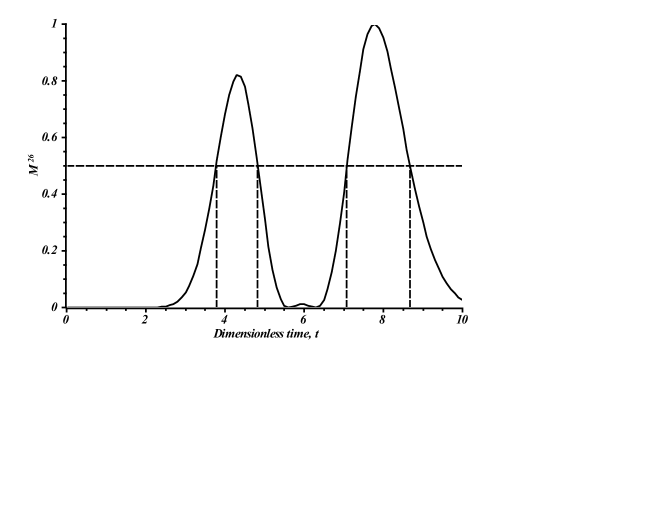
Figure 1: The function $M^{26}(t)$ given by eq.(168) with $M^{26}_{max}=1.247\times 10^{-11}$ and $\displaystyle\varepsilon=\frac{\pi}{160}$; there are two time intervals corresponding to $\displaystyle M^{26}(t)>\frac{1}{2}$: $3.781<t<4.827$ and $7.082<t<8.678$.

We see that the function ${{M}}^{26}(t)$ is positive during the rather long time intervals. However, the time intervals corresponding to very small values of this function must be disregarded because of the possible obstacles to detect parameters $\varphi_{i}$ ($i=2,6$) during these intervals (for instance , because of fluctuations). For this reason, we suggest to use time intervals corresponding to $\displaystyle M^{26}>\frac{1}{2}$. Fig.1 shows that there are two such subintervals inside of the selected interval $0<t<10$: $3.781<t<4.827$ and $7.082<t<8.678$. Thus, we calculate the non-reducible informational correlation provided by the parameters $\varphi_{2}$ and $\varphi_{6}$ from $\hat{g}$ (167) with zero values of other parameters and eigenvalues (162): $E^{AB;min}(\hat{g},t)=2$ inside of the two above time subintervals (remember that $\displaystyle\lambda^{B}_{i}=\frac{1}{4}$, $i=1,2,3,4$, in this example because ${\mbox{ran}}\,\hat{T}=7$).

Example 2: ${\mbox{ran}}\,\hat{T}=9$, $E^{AB}=6$ in Table 2.

In accordance with Table 2, $E^{AA}=6$. Using formula (81) for $H$, we obtain that the third order minors of the $3\times 6$ matrix $H$ are nonzero, so that eq.(82) yields $E^{AB;min}=3$. The analysis of the third-order minors shows that any triad of the parameters $\varphi_{i}$, $i=1,\dots,6$ may be transfered from the subsystem $A$ to the subsystem $B$ by the eigenvalues of the density matrix $\rho^{B}(\varphi^{A},t)$ except for the triad of the parameters $\varphi_{1},\varphi_{3},\varphi_{5}$. These parameters are introduced by the diagonal matrix exponents $e^{i\gamma_{3}\varphi_{i}}$ ($i=1,3,5$) in the unitary transformation (145) .

Similar to the previous example, we consider the informational correlation established by the one triad of the parameters, namely $\varphi_{2}$, $\varphi_{4}$, $\varphi_{6}$, putting other parameters to zero. Thus the restricted set of parameters is $\hat{\varphi}^{A}=\{\varphi_{2},\varphi_{4},\varphi_{6}\}$. Therewith we take $\hat{\varphi}^{A}\in\hat{G}^{A}$ where $\displaystyle\hat{G}^{A}:0<\varphi_{2},\varphi_{4},\varphi_{6}<\frac{\pi}{2}$. We also fix eigenvalues as follows:

$$\displaystyle\lambda^{A}_{1}=\lambda^{A}_{2}=\lambda^{A}_{3}=\frac{4}{15},\;\;\displaystyle\lambda^{A}_{4}=\frac{1}{5},$$ (176)

$$\displaystyle\lambda^{B}_{1}=\lambda^{B}_{2}=\frac{4}{15},\;\;\displaystyle\lambda^{B}_{3}=\displaystyle\lambda^{B}_{4}=\frac{7}{30}.$$

In this case, only the second, the fourth and the sixth columns of the matrix $H(t)$ (81) are nonzero so that we may replace $H$ by the following $3\times 3$ matrix $\tilde{H}$:

$$\tilde{H}(\varphi_{2},\varphi_{4},\varphi_{6},t)=\left(\begin{array}[]{ccc}\displaystyle\frac{\partial a_{0}(\varphi_{2},\varphi_{4},\varphi_{6},t)}{\partial\varphi_{2}}&\displaystyle\frac{\partial a_{0}(\varphi_{2},\varphi_{4},\varphi_{6},t)}{\partial\varphi_{4}}&\displaystyle\frac{\partial a_{0}(\varphi_{2},\varphi_{4},\varphi_{6},t)}{\partial\varphi_{6}}\cr\displaystyle\frac{\partial a_{1}(\varphi_{2},\varphi_{4},\varphi_{6},t)}{\partial\varphi_{2}}&\displaystyle\frac{\partial a_{1}(\varphi_{2},\varphi_{4},\varphi_{6},t)}{\partial\varphi_{4}}&\displaystyle\frac{\partial a_{1}(\varphi_{2},\varphi_{4},\varphi_{6},t)}{\partial\varphi_{6}}\cr\displaystyle\frac{\partial a_{2}(\varphi_{2},\varphi_{4},\varphi_{6},t)}{\partial\varphi_{2}}&\displaystyle\frac{\partial a_{2}(\varphi_{2},\varphi_{4},\varphi_{6},t)}{\partial\varphi_{4}}&\displaystyle\frac{\partial a_{2}(\varphi_{2},\varphi_{4},\varphi_{6},t)}{\partial\varphi_{6}}\end{array}\right).$$ (180)

Similar to the previous example, we define the region $\hat{g}\subset\hat{G}^{A}$ as

$$\hat{g}:\varepsilon<\varphi_{2},\varphi_{4},\varphi_{6}<\frac{\pi}{2}-\varepsilon.$$ (181)

Let us consider the informational correlation during the time interval $0\leq t\leq 10$ using the parameters inside of the region (181). To find out the time intervals where all three parameters $\varphi_{i}$, $i=2,4,6$, may be detected, we construct the function ${{M}}^{246}(t)$ defined by the following formula (similar to eq.(168)):

$${{M}}^{246}(t)=\frac{M^{246}_{3}(t)}{M^{246}_{max}},\;\;M^{246}_{3}(t)=\min_{\varphi_{2},\varphi_{4},\varphi_{6}\in\hat{g}}|M^{246}_{31}(\varphi_{2},\varphi_{4},\varphi_{6},t)|,\;\;M^{246}_{max}=\max\limits_{0\leq t\leq T}M^{246}_{3}(t),$$ (182)

where the minimization is over the parameters $\varphi_{2}$, $\varphi_{4}$ and $\varphi_{6}$ inside of the region $\hat{g}$, and the only nonzero 3rd order minor of $\tilde{H}$ is $\det\,\tilde{H}$, i.e., $M^{246}_{31}=\det\,\tilde{H}$. The function ${{M}}^{246}(t)$ with $\displaystyle\varepsilon=\frac{\pi}{50}$ is depicted in Fig.2. Similar to the previous example, we select the time intervals with $\displaystyle M^{246}>\frac{1}{2}$ as the suitable intervals for the parameter detection. We see that there are two such subintervals inside of the interval $0<t<10$: $3.257<t<4.520$ and $7.233<t<7.983$. Thus we calculate the non-reducible informational correlation provided by the parameters $\varphi_{2}$, $\varphi_{4}$ and $\varphi_{6}$ from $\hat{g}$ (181) with zero values of other parameters and eigenvalues (176): $E^{AB;min}(\hat{g},t)=3$ inside of the two above time subintervals (remember that $\lambda^{B}_{i}$ satisfy either conditions (154,156) or conditions (155,157)).

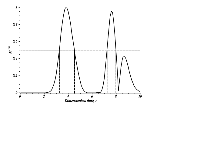
Figure 2: The function $M^{246}(t)$ given by eq.(182)) with $M^{246}_{max}=2.292\times 10^{-25}$, $\displaystyle\varepsilon=\frac{\pi}{50}$; there are two time intervals corresponding to $\displaystyle M^{246}(t)>\frac{1}{2}$: $3.257<t<4.520$ and $7.233<t<7.983$

4 Informational correlations in long spin-1/2 chains: particular examples

Results of Sec.3 allow us to conclude that there are two basic obstacles in calculation of the informational correlation. First, we have to calculate the Jacobian (48) using the formula (52). The matrix dimensionality of this Jacobian increases with the increase in $N^{B}$ as $((N^{A})^{2}-1)\tilde{D}=((N^{A})^{2}-1)N^{A}(N^{A}-1)$. Second, the calculation of the operator $T(t)$ in eq.(52) is a very complicated dynamical problem for the long chains. In fact, the dynamics of the $N$-node chain is described in the $2^{N}$-dimensional Hilbert space and may be simulated only for small $N$ in general. However, the evolution of single excited spin along the spin-1/2 chain governed by the Hamiltonian commuting with the $z$-projection $I_{z}$ of the total spin momentum is an exception. In this case, the $N$-node chain evolves in the ($N+1$)-dimensional Hilbert space.

This chain was considered in [36], where, in addition, the approximation of nearest neighbor interaction was used. Namely this model serves us as a model of the long spin-1/2 chain establishing the maximal possible informational correlation between the first and the last nodes which we call subsystems $A$ and $B$, respectively (the remaining $N-2$ nodes compose the subsystem $C$ in this case). Since $A$ is a one-node subsystems, the group $SU(2)$ represents a group of unitary operators locally acting on this subsystem.

Emphasize that the case of pure initial states considered in this section allows us to simplify formulas of Sec.2 replacing the density matrix elements with the transition amplitudes. It is also important that, in the case of pure initial state with a single excitation in the subsystem $A$, the reduced density matrix of the subsystem $A$ has only one non-zero eigenvalue and it equals to unit (i.e., the state of the subsystem $A$ is pure): $\Lambda={\mbox{diag}}(1,0,\dots,0)$. Consequently, such initial state of the subsystem $A$ may be represented as $\rho^{A}=U(\varphi^{A})\Lambda U^{+}(\varphi^{A})$. Thus, all independent arbitrary parameters appearing below in the pure states (184) and (191) are associated with parameters of the unitary transformation.

Let us use the following conventional basis [36]:

$$|\mathbf{j}\rangle,\;\;\mathbf{j}=\mathbf{0},\mathbf{1},\dots,\mathbf{N},$$ (183)

where ${j}$ means the location of the excited node (i.e., the $j$th node is directed opposite to the external magnetic field) while all other nodes are in the basic state (i.e., they are directed along the external field). Therewith $\mathbf{0}$ means that all nodes are in the basic state. If we deal with a single node (subsystems $A$ or $B$) we use notation $|0\rangle$ for the spin in the basic state and $|1\rangle$ for the excited spin.

Two transferable parameters of the $SU(2)$ are incorporated into the arbitrary initial state of the first spin [36] as follows:

$$|\psi_{1}(0)\rangle=\cos\frac{\varphi_{1}}{2}|0\rangle+e^{i\varphi_{2}}\sin\frac{\varphi_{1}}{2}|1\rangle.$$ (184)

The initial density matrix $\rho^{A}(\varphi^{A})$ reads

$$\rho^{A}(\varphi^{A})=|\psi_{1}(0)\rangle\langle\psi_{1}(0)|.$$ (185)

Thus, $E^{AA}=2$, $E^{AA}_{norm}=1$, i.e., the information encoded into the subsystem $A$ reaches its maximal possible value as is shown in Sec.2, eq.(43) (see also Sec.3.1.1). Although the initial state of the whole system is pure, the state of the $N$th node is a mixed one and is described by the following reduced density matrix [36]:

$$\rho^{B}(t)=P(t)|\psi^{B}(t)\rangle\langle\psi^{B}(t)|+(1-P(t))|0\rangle\langle 0|,$$ (186)

where

$$|\psi^{B}(t)\rangle=\frac{1}{\sqrt{P(t)}}\left(a_{1}(\varphi_{1})|0\rangle+a_{2}(\varphi_{1},\varphi_{2},t)|1\rangle\right),$$ (187)

$$a_{1}(\varphi_{1})=\cos\frac{\varphi_{1}}{2},\;\;a_{2}(\varphi_{1},\varphi_{2},t)=e^{i\phi_{2}}\sin\frac{\varphi_{1}}{2}f^{N}_{AB}(t),$$

$$P(t)=\cos^{2}\frac{\varphi_{1}}{2}+\sin^{2}\frac{\varphi_{1}}{2}|f^{N}_{AB}(t)|^{2},$$

$$f^{N}_{AB}(t)=\langle\mathbf{N}|e^{-iHt}|\mathbf{1}\rangle.$$

Here $f^{N}_{AB}(t)$ is the transition amplitude of an excitation from the 1st to the $N$th spin, $|\mathbf{1}\rangle$ and $|\mathbf{N}\rangle$ mean the states with the first and last excited spin respectively (in accordance with eq.(183)), and $H$ is the Hamiltonian governing the dynamics of the spin chain with the only restriction $[H,I_{z}]=0$. Having the parameters $a_{i}$, $i=1,2$, we may find two real parameters $\varphi_{i}$, $i=1,2$ solving the following system of one real and one complex equations (i.e., the system is overdetermined but compatible):

$$a_{1}=\cos\frac{\varphi_{1}}{2},\;\;a_{2}=e^{i\phi_{2}}\sin\frac{\varphi_{1}}{2}f^{N}_{AB}(t).$$ (188)

This system is solvable at any instant satisfying the condition

$$f^{N}_{AB}(t)\neq 0.$$ (189)

Therewith $P(t)>0$ by definition. Thus, the maximal possible informational correlation $E^{AB}=2$ ($E^{AB}_{norm}=1$) is established between one-node subsystems $A$ and $B$ (the first and the last nodes of the $N$-node spin chain). At such time moments that $f^{N}_{AB}(t)=0$, only the first of eqs.(188) remains, so that $E^{AB}=1$ ($E^{AB}_{norm}=1/2$).

Now we show how the system with a single excited node may be used to establish the informational correlation between the large subsystems $A$ and $B$. It is convenient to use the following notations for the basis vectors of the $M$-node subsystem.

$$|\mathbf{j}_{M}\rangle,\;\;\mathbf{j}=\mathbf{0},\mathbf{1},\dots,\mathbf{M},$$ (190)

where we explicitly use the length $M$ of the selected subsystem. Let the subsystems $A$ and $B$ of the $N$-node spin chain consist of $\tilde{N}^{A}$ first nodes and $\tilde{N}^{B}$ last nodes respectively. We generalize the initial state (184) as follows:

$$|\psi^{A}(0)\rangle=\alpha_{0}|\mathbf{0}_{\tilde{N}^{A}}\rangle+\sum_{j=1}^{\tilde{N}^{A}}\alpha_{j}|\mathbf{j}_{\tilde{N}^{A}}\rangle,$$ (191)

where $\alpha_{0}$ may be taken as a real parameter and parameters $\alpha_{j}$, $j>0$, are the complex ones with the normalization

$$\alpha_{0}^{2}+\sum_{i=1}^{\tilde{N}^{A}}|\alpha_{i}|^{2}=1.$$ (192)

We require that all other spins are in the basic state, i.e., the initial state of the whole system reads:

$$|\psi(0)\rangle=|\psi^{A}(0)\rangle\otimes|\mathbf{0}_{N-\tilde{N}^{A}}\rangle,$$ (193)

where $|\mathbf{0}_{N-\tilde{N}^{A}}\rangle$ means the basic state of the chain of ${N-\tilde{N}^{A}}$ nodes.

Thus, all in all, we have $2\tilde{N}^{A}$ arbitrary real parameters: $2\tilde{N}^{A}+1$ parameters $a_{0}$, ${\mbox{Re}}\alpha_{i}$, ${\mbox{Im}}\alpha_{i}$, $i=1,\dots,\tilde{N}^{A}$ related by the normalization condition (192). As shown in the beginning of this section, these arbitrary parameters are associated with $2\tilde{N}^{A}$ arbitrary parameters $\varphi_{i}$ of the unitary transformation. For simplicity, we do not explicitly write this dependence in the arguments of $\alpha_{i}$. Thus, $E^{AA}=2\tilde{N}^{A}$, $\displaystyle E^{AA}_{norm}=\frac{2\tilde{N}^{A}}{2^{\tilde{N}^{A}}(2^{\tilde{N}^{A}}-1)}$. Of course, the found $E^{AA}$ is less then the maximal possible number of parameters that may be encoded into the mixed initial state of the subsystem $A$ consisting of $\tilde{N}^{A}$ nodes considered in Sec.2. Thus, the subsystems $A$ and $B$ may not possess the maximal possible informational correlation (which is $E^{AA}=2^{\tilde{N}^{A}}(2^{\tilde{N}^{A}}-1)$) using the pure initial state (191) and the Hamiltonian commuting with $I_{z}$.

With time, the initial state of the whole system (193) evolves as follows:

$$|\psi(t)\rangle=e^{-iHt}|\psi^{A}(0)\rangle\otimes|\mathbf{0}_{N-\tilde{N}^{A}}\rangle.$$ (194)

The state of the subsystem $B$ is described by the following reduced density matrix

$$\rho^{B}_{\tilde{N}^{B}}(t)=P_{\tilde{N}^{B}}(t)|\psi^{B}_{\tilde{N}^{B}}(t)\rangle\langle\psi^{B}_{\tilde{N}^{B}}(t)|+(1-P_{\tilde{N}^{B}}(t))|0\rangle\langle 0|$$ (195)

where

$$|\psi^{B}_{\tilde{N}^{B}}(t)\rangle=\frac{1}{\sqrt{P_{\tilde{N}^{B}}(t)}}\left(\beta_{0}|\mathbf{0}_{\tilde{N}^{B}}\rangle+\sum_{j=1}^{N^{B}}\beta_{j}|\mathbf{j}_{\tilde{N}^{B}}\rangle\right),$$ (196)

$\beta_{i}$ are the transition amplitudes:

$$\beta_{0} = \left(\langle\mathbf{0}_{N-\tilde{N}^{B}}|\otimes\langle\mathbf{0}_{\tilde{N}^{B}}|\right)|\psi(t)\rangle=\alpha_{0}$$ (197)

$$\beta_{j} = \left(\langle\mathbf{0}_{N-\tilde{N}^{B}}|\otimes\langle\mathbf{j}_{\tilde{N}^{B}}|\right)|\psi(t)\rangle=\sum_{k=1}^{\tilde{N}^{A}}\alpha_{k}r_{jk},$$ (199)

$$r_{jk}=\langle\mathbf{j}_{\tilde{N}^{B}}|\otimes\langle\mathbf{0}_{N-\tilde{N}^{B}}|e^{-iHt}|\mathbf{k}_{\tilde{N}^{A}}\rangle\otimes|\mathbf{0}_{N-\tilde{N}^{A}}\rangle,$$

and $P_{\tilde{N}^{B}}(t)$ is the normalization:

$$P_{\tilde{N}^{B}}(t)=\beta_{0}^{2}+\sum_{j=1}^{N^{B}}|\beta_{j}|^{2}.$$ (200)

Thus, we may register at most $2\tilde{N}^{B}$ real parameters in the subsystem $B$, i.e., $E^{AB}(t)\leq 2\tilde{N}^{B}$,$\displaystyle E^{AB}_{norm}(t)\leq\frac{2\tilde{N}^{B}}{2^{\tilde{N}^{B}}(2^{\tilde{N}^{B}}-1)}$. Let us use the transition amplitudes $\beta_{j}$, $j=0,1,\dots,\tilde{N}^{B}$, rather then the density matrix elements to calculate the number of transfered parameters $\varphi_{i}$ and write system (197,199) in the matrix form:

$$\boldsymbol{\beta}=\boldsymbol{T\,\alpha},$$ (201)

where

$$\boldsymbol{\beta}=(\beta_{0},\beta_{1},\dots,\beta_{\tilde{N}^{B}})^{T},\;\;\boldsymbol{\alpha}=(\alpha_{0},\dots,\alpha_{\tilde{N}^{A}})^{T},\;\;$$ (202)

$$\mathbf{T}=\left(\begin{array}[]{cccc}1&0&\cdots&0\cr 0&r_{11}&\cdots&r_{1\tilde{N}^{A}}\cr\cdots&\cdots&\cdots&\cdots\cr 0&r_{\tilde{N}^{B}1}&\cdots&r_{\tilde{N}^{B}\tilde{N}^{A}}\end{array}\right).$$ (207)

Equation (201) is the analogue of equation (15) in Sec.2. Let $\tilde{N}^{A}=\tilde{N}^{B}$ hereafter in this section. Then, $\mathbf{T}$ is a square matrix and the condition

$$\det\boldsymbol{T}\neq 0$$ (208)

provides the complete information transfer. Consequently, the maximal informational correlation between the subsystems $A$ and $B$ is reached: $E^{AB}_{max}=2\tilde{N}^{A}$, $\displaystyle E^{AB}_{norm}(t)=\frac{2\tilde{N}^{A}}{2^{\tilde{N}^{A}}(2^{\tilde{N}^{A}}-1)}$.

For the further study, let us split the real and imaginary parts of eq. (201) and rewrite this equation as

$$\left(\begin{array}[]{c}{\mbox{Re}}\;\boldsymbol{\beta}\cr{\mbox{Im}}\;\boldsymbol{\beta}\end{array}\right)=\hat{\boldsymbol{T}}\left(\begin{array}[]{c}{\mbox{Re}}\;\boldsymbol{\alpha}\cr{\mbox{Im}}\;\boldsymbol{\alpha}\end{array}\right),\;\;\;\hat{\boldsymbol{T}}=\left(\begin{array}[]{cc}{\mbox{Re}}\;\boldsymbol{T}&-{\mbox{Im}}\;\boldsymbol{T}\cr{\mbox{Im}}\;\boldsymbol{T}&{\mbox{Re}}\;\boldsymbol{T}\end{array}\right).$$ (215)

Eq.(215) is an analogue of eq.(40) in Sec.2. We see, that the number of real equations in system (215) is $2\tilde{N}^{A}+1$. This is one grater then the number of independent parameters $\varphi_{i}$ that may be found from system (215). Thus, similar to the mixed initial state case considered in Sec.2, condition (208) is enough, but it is not a necessary condition for the maximal possible informational correlation. If $\det\boldsymbol{T}=0$, then the parameter $E^{AB}$ is defined by the rank of $\boldsymbol{T}$. In turn, this rank is defined by the particular choice of the spin chain length and Hamiltonian. Formally, the maximal possible informational correlation $E^{AB}$ may be achieved for ${\mbox{ran}}\,\hat{\boldsymbol{T}}\geq 2\tilde{N}^{A}$. Otherwise, we deal with the partial information correlation. Further examples of informational correlations in quantum systems will be given in different paper.

Non-reducible informational correlation. Regarding the non-reducible informational correlation, it is unit in the considered examples. In fact, both reduced density matrices (186) and (195) are written in the diagonal form and have two nonzero eigenvalues: $P,(1-P)$ and $P_{\tilde{N}^{B}},(1-P_{\tilde{N}^{B}})$ respectively. Thus only one parameter may be transfered by the eigenvalues of the reduced density matrix associated with the subsystem $B$, i.e., $E^{AB;min}=1$, $\displaystyle E^{AB;min}_{norm}=\frac{1}{2^{\tilde{N}^{A}}(2^{\tilde{N}^{A}}-1)}$.

5 Conclusions

We introduce the informational correlation between two subsystems $A$ and $B$ as the possibility to effect on the state of the subsystem $B$ through the parameters of the unitary transformation $U^{A}$ locally performed on the subsystem $A$ and vice-versa. The measure of the informational correlation $E^{AB}$ equals to the number of parameters of the local unitary transformation $U^{A}$ which may be detected in the subsystem $B$. We also introduce the normalized measure of the informational correlation $E^{AB}_{norm}$ showing whether the informational correlation is far from the saturation. The so-called non-reducible informational correlation $E^{AB;min}(t)$ is of a special interest, because this part of informational correlation is invariant with respect to the local unitary transformations of the subsystem $B$ at the time instant $t$.

Below we represent the list of the basic properties of the informational correlation (for the tensor product initial density matrix (13)) and compare them with the analogous properties of the discord and entanglement (if this is possible).

1. Unlike the entanglement and discord, the informational correlation represents a dynamical characteristics which is identical to zero at the initial time instant.

2. By its definition (49) in terms of the rank of some Jacobian matrix, the informational correlation takes the discrete set of values, unlike the entanglement and discord. Moreover, this definition provides the stability of the informational correlation with respect to deviations of the system’s parameters (such as the dipole-dipole interaction constants and the magnetic field distribution).

3. The informational correlation is invariant with respect to the initial local unitary transformations of the subsystem $A$, similar to the usual entanglement and discord. However, the informational correlation is not invariant with respect to the local unitary transformations of the subsystem $B$ (either initial or $t$-dependent), unlike the entanglement and discord. Consequently, using the local unitary transformations of the receiver $B$ we may handle (up to a certain extent) the number of the parameters transfered from the subsystem $A$ to the subsystem $B$ and, thus, manipulate the informational correlation $E^{AB}$. The local transformations performed on the subsystem $C$ may also effect $E^{AB}$.

4. $E^{AB}(t)\equiv 0$ only if the initial density matrix $\rho^{A}(0)$ in formula (13) is proportional to the identity matrix. For the tensor product initial state (13,46), $E^{AB}=E^{BA}=0$ only if both $\rho^{A}(0)$ and $\rho^{B}(0)$ are proportional to the identity matrix. The unitary invariant discord possesses the same property [29].

5. The complete information transfer is not required in order to obtain the maximal possible value of $E^{AB}$, because the maximal possible number of arbitrary parameters $\varphi_{i}$ transfered from $A$ to $B$ is less then $(N^{A})^{2}-1$ (the maximal number of different real parameters in the $N^{A}\times N^{A}$ density matrix).

6. The informational correlation is sensitive to the multiplicity of the eigenvalues of the matrices $\rho^{A}(0)$ and $\rho^{B}(0)$ for the case of the tensor product initial state (13,46).

7. It is interesting that the conditions $E^{AA}<\tilde{D}^{A}$ and $E^{AB}<E^{AA}$ require the strong relations among the eigenvalues $\lambda^{A}_{i}$, $\lambda^{B}_{i}$ and $\lambda^{C}_{i}$. For the particular examples, these relations have been found in Sec.3, see eqs.(110,151,154,155) and Tables 1,2. The minor deviation from these exact relations leads (i) to the encoding of the maximal possible parameters $\tilde{D}^{A}$ into the subsystem $A$ and (ii) to the spread of the complete information throughout the whole system and consequently to the maximal possible informational correlation $E^{AB}=E^{AA}=\tilde{D}^{A}$. This phenomenon was not observed in the case of entanglement and discord. Presumably, such behavior of a system must be closely related with the fluctuations of the informational correlation and requires the more detailed study.

8. There are two subsets of parameters $\varphi_{i}$ transfered from $A$ to $B$: $\varphi^{U}$ and $\varphi^{\Lambda}$. The first one may be detected in the matrix of the eigenvectors of the reduced density matrix $\rho^{B}(\varphi^{A},t)$, while the second subset is transfered by the eigenvalues of the same matrix. The subset $\varphi^{\Lambda}$ is most reliable for the purpose of the information transfer, because the number of parameters in this subset may not be decreased by any local unitary transformation performed on the subsystem $B$. Namely this subset is responsible for the non-reducible informational correlation $E^{AB;min}$. Note that some of the parameters $\varphi_{i}$ might be encoded in both subsets $\varphi^{U}$ and $\varphi^{\Lambda}$. The informational correlation $E^{AB}$ and the non-reducible informational correlation $E^{AB;min}$ might be viewed as the analogues of the total and the classical correlations in the definition of the discord. The removable informational correlation $\Delta E^{AB}=E^{AB}-E^{AB;min}$ is the analogue of the discord itself.

9. Presumably, the case of non-separable initial state will reveal some additional interesting features. For instance, the informational correlations established by the subgroup of LNUs [30, 31, 32] should be studied.

10. Parameters of the group $SU(N^{A})$ transfered form $A$ to $B$ may be treated as bits of information. Local transformations of the subsystems $B$ (and perhaps $C$) provide a control of information transfer. These two facts suggest us to consider a bi-partite (or three-partite) quantum system with local transformations as a controllable gate or chain of gates (if the subsystems are large enough). In the case of 1-spin subsystems $A$ and $B$ we have 2 parameters (which might be treated, for instance, as 2 bits). The 2-spin subsystems provide us with 12 bits. In general, $n$-node subsystems $A$ and $B$ of spin-1/2 particles yield $(2^{2n}-2^{n})$ bits. The introduced measure $E^{AB}$ allows us to handle the remote control of gates. Both the gate construction and the remote control of gates are those problems that deserve the further study.

11. We represent the detailed study of the informational correlations (including the non-reducible ones) between the one- and two-node subsystems $A$ and $B$ in the four node spin-1/2 chain with mixed initial states governed by the XY Hamiltonian, Sec.3. The informational correlation may be relatively simply calculated in the spin-1/2 chains having a pure initial state with single initially excited node of the subsystem $A$ provided that the spin dynamics is governed by the Hamiltonian commuting with $I_{z}$ ( $z$-projection of the total spin momentum), as is shown in Sec.4. The case of one-particle subsystems $A$ and $B$ is studied in details; general formulas for the calculation of informational correlation between arbitrary subsystems $A$ and $B$ of long chain are derived. The non-reducible informational correlation equals one for this type of initial states.

Finally we would like to notice that, although there is no apparent relation between the informational correlation and LE, the idea of increasing the amount of correlations between two selected particles by doing local measurements on the rest of quantum system [19, 20] may be used in the further development of application of informational correlation.

Author thanks Profs. E.B.Fel’dman, M.A.Yurishchev and Dr. A.N.Pyrkov for useful discussion. Author also thanks reviewer for useful comment. This work is partially supported by the Program of the Presidium of RAS No.8 ”Development of methods of obtaining chemical compounds and creation of new materials” and by the RFBR grant No.13-03-00017

6 Appendix

6.1 A. Explicit form of the matrices $\gamma_{i}$.

We give the list of matrices $\gamma_{i}$ representing the basis of the Lie algebra of $SU(4)$ [35]:

$$\gamma_{1}=\left[\begin{array}[]{cccc}0&1&0&0\cr 1&0&0&0\cr 0&0&0&0\cr 0&0&0&0\end{array}\right],\;\;\gamma_{2}=\left[\begin{array}[]{cccc}0&-i&0&0\cr i&0&0&0\cr 0&0&0&0\cr 0&0&0&0\end{array}\right],\;\;\gamma_{3}=\left[\begin{array}[]{cccc}1&0&0&0\cr 0&-1&0&0\cr 0&0&0&0\cr 0&0&0&0\end{array}\right],$$ (228)

$$\gamma_{4}=\left[\begin{array}[]{cccc}0&0&1&0\cr 0&0&0&0\cr 1&0&0&0\cr 0&0&0&0\end{array}\right],\;\;\gamma_{5}=\left[\begin{array}[]{cccc}0&0&-i&0\cr 0&0&0&0\cr i&0&0&0\cr 0&0&0&0\end{array}\right],\;\;\gamma_{6}=\left[\begin{array}[]{cccc}0&0&0&0\cr 0&0&1&0\cr 0&1&0&0\cr 0&\;\;0&0&0\end{array}\right],$$ (241)

$$\gamma_{7}=\left[\begin{array}[]{cccc}0&0&0&0\cr 0&0&-i&0\cr 0&i&0&0\cr 0&0&0&0\end{array}\right],\;\;\gamma_{8}=\frac{1}{\sqrt{3}}\left[\begin{array}[]{cccc}1&0&0&0\cr 0&1&0&0\cr 0&0&-2&0\cr 0&0&0&0\end{array}\right],\;\;\gamma_{9}=\left[\begin{array}[]{cccc}0&0&0&1\cr 0&0&0&0\cr 0&0&0&0\cr 1&0&0&0\end{array}\right],$$ (254)

$$\gamma_{10}=\left[\begin{array}[]{cccc}0&0&0&-i\cr 0&0&0&0\cr 0&0&0&0\cr i&0&0&0\end{array}\right],\;\;\gamma_{11}=\left[\begin{array}[]{cccc}0&0&0&0\cr 0&0&0&1\cr 0&0&0&0\cr 0&1&0&0\end{array}\right],\;\;\gamma_{12}=\left[\begin{array}[]{cccc}0&0&0&0\cr 0&0&0&-i\cr 0&0&0&0\cr 0&i&0&0\end{array}\right],$$ (267)

$$\gamma_{13}=\left[\begin{array}[]{cccc}0&0&0&0\cr 0&0&0&0\cr 0&0&0&1\cr 0&0&1&0\end{array}\right],\;\;\gamma_{14}=\left[\begin{array}[]{cccc}0&0&0&0\cr 0&0&0&0\cr 0&0&0&-i\cr 0&0&i&0\end{array}\right],\;\;\gamma_{15}=\frac{1}{\sqrt{6}}\left[\begin{array}[]{cccc}1&0&0&0\cr 0&1&0&0\cr 0&0&1&0\cr 0&0&0&-3\end{array}\right].$$ (280)

6.2 B. Proof of eq.(82) for multiple and zero eigenvalues $\lambda_{i}$ of the matrix $\rho^{B}(\varphi^{A},t)$

Suppose that there are $(P+1)<(N^{B}-1)$ nonzero different eigenvalues of the matrix $\rho^{B}(\varphi,t)$. Then, in order to define the non-reducible informational correlation $E^{AB;min}$, we may replace the characteristic equation (65) with the following polynomial one:

$$\prod_{i=1}^{P}(\lambda-\lambda_{i}(\varphi^{A},t))=\lambda^{P}+\sum_{j=0}^{P-1}\tilde{a}_{i}(\varphi^{A},t)\lambda^{i}=0,$$ (281)

where $\tilde{a}_{i}$ are expressed in terms of $\lambda_{i}$. In this equation, we take into account only $P$ different nonzero eigenvalues because of the identity $\displaystyle{\mbox{Tr}}\rho^{B}=\sum\limits_{i=1}^{P+1}q_{i}\lambda_{i}=1$, where $q_{i}$ is the multiplicity of the root $\lambda_{i}$. Then the non-reducible informational correlation is defined by the rank of the matrix

$$J^{B}_{\Lambda}(\varphi^{A},t)=\frac{\partial(\lambda_{1}(\varphi^{A},t),\dots,\lambda_{P}(\varphi^{A},t))}{\partial(\varphi_{1},\dots,\varphi_{\tilde{D}^{A}})},$$ (282)

so that

$$E^{AB;min}(\varphi^{A},t)={\mbox{ran}}\,J^{B}_{\Lambda}(\varphi^{A},t).$$ (283)

Differentiating eq.(281) with respect to the parameters $\varphi_{k}$, $k=1,\dots,\tilde{D}^{A}$, and solving the resulting equations for $\displaystyle\frac{\partial\lambda}{\partial\varphi_{k}}$ we obtain:

$$\frac{\partial\lambda}{\partial\varphi_{k}}=-\frac{\displaystyle\sum_{i=0}^{P-1}\frac{\partial\tilde{a}_{i}(\varphi^{A},t)}{\partial\varphi_{k}}\lambda^{i}}{\displaystyle P\lambda^{P-1}+\sum_{i=1}^{P-1}i\tilde{a}_{i}(\varphi^{A},t)\lambda^{i-1}}.$$ (284)

Therefore, for the matrix $J^{B}_{\Lambda}(\varphi^{A},t)$ one has

$$J^{B}_{\Lambda}(\varphi^{A},t) = \frac{1}{\tilde{J}_{0}(\varphi^{A},t)}\left(\begin{array}[]{ccc}\displaystyle\sum_{i=0}^{P-1}\frac{\partial\tilde{a}_{i}(\varphi^{A},t)}{\partial\varphi_{1}}\lambda^{i}_{1}(\varphi^{A},t)&\cdots&\displaystyle\sum_{i=0}^{P-1}\frac{\partial\tilde{a}_{i}(\varphi^{A},t)}{\partial\varphi_{\tilde{D}^{A}}}\lambda^{i}_{1}(\varphi^{A},t)\cr\cdots&\cdots&\cdots\cr\displaystyle\sum_{i=0}^{P-1}\frac{\partial\tilde{a}_{i}(\varphi^{A},t)}{\partial\varphi_{1}}\lambda^{i}_{P}(\varphi^{A},t)&\cdots&\displaystyle\sum_{i=0}^{P-1}\frac{\partial\tilde{a}_{i}(\varphi^{A},t)}{\partial\varphi_{\tilde{D}^{A}}}\lambda^{i}_{P}(\varphi^{A},t)\end{array}\right)=$$ (289)

$$\tilde{\Lambda}^{B}(\varphi^{A},t)\tilde{H}(\varphi^{A},t),$$

where

$$\tilde{J}_{0}(\varphi^{A},t)=(-1)^{P}\prod_{j=1}^{P}\Big{(}P\lambda^{P-1}_{j}(\varphi^{A},t)+\sum_{i=1}^{P-1}i\tilde{a}_{i}(\varphi^{A},t)\lambda^{i-1}_{j}(\varphi^{A},t)\Big{)}\neq 0,$$ (290)

while $\tilde{\Lambda}^{B}$ and $\tilde{H}$ are the $P\times P$ and $P\times\tilde{D}^{A}$ matrices respectively:

$$\tilde{\Lambda}^{B}=\left(\begin{array}[]{cccc}\displaystyle 1&\lambda_{1}(\varphi^{A},t)&\cdots&\lambda_{1}^{P-1}(\varphi^{A},t)\cr\cdots&\cdots&\cdots&\cdots\cr 1&\lambda_{P}(\varphi^{A},t)&\cdots&\lambda_{P}^{P-1}(\varphi^{A},t)\end{array}\right),$$ (294)

$$\tilde{H}(\varphi^{A},t)=\left(\begin{array}[]{ccc}\displaystyle\frac{\partial\tilde{a}_{0}(\varphi^{A},t)}{\partial\varphi_{1}}&\cdots&\displaystyle\frac{\partial\tilde{a}_{0}(\varphi^{A},t)}{\partial\varphi_{\tilde{D}^{A}}}\cr\cdots&\cdots&\cdots\cr\displaystyle\displaystyle\frac{\partial\tilde{a}_{P-1}(\varphi^{A},t)}{\partial\varphi_{1}}&\cdots&\displaystyle\frac{\partial\tilde{a}_{P-1}(\varphi^{A},t)}{\partial\varphi_{\tilde{D}^{A}}}\end{array}\right).$$ (298)

Then eq.(283) yields

$$E^{AB;min}(\varphi^{A},t)={\mbox{ran}}\,J^{B}_{\Lambda}(\varphi^{A},t)={\mbox{ran}}\,\tilde{H}(\varphi^{A},t).$$ (299)

Now notice that $P$ coefficients $\tilde{a}_{i}$ in eq.(281) are defined by $P$ different nonzero eigenvalues $\lambda_{i}$, $i=1,\dots,P$. From another hand, the coefficients $a_{i}$ in eq.(65) are defined by the same $P$ independent eigenvalues $\lambda_{i}$, $i=1,\dots,P$, and consequently by $P$ coefficients $\tilde{a}_{i}$, $i=1,\dots,P$. The last statement is provided by the relation between sets $\tilde{a}_{i}$ and $\lambda_{i}$. This relation follows from eq.(281), where all $\lambda_{i}$, $i=1,\dots,\lambda_{P}$, are different by our requirement. Consequently,

$$\left|\frac{\partial(\tilde{a}_{0},\dots,\tilde{a}_{P-1})}{\partial(\lambda_{1},\dots,\lambda_{P})}\right|\neq 0.$$ (300)

Thus, for the matrix $H$ represented by eq.(81), we may write

$$H(\varphi^{A},t)=F(\varphi^{A},t)\tilde{H}(\varphi^{A},t),$$ (301)

where $F$ is $(N^{B}-1)\times P$ matrix,

$$F(\varphi^{A},t)=\left(\begin{array}[]{ccc}\displaystyle\frac{\partial a_{0}(\varphi^{A},t)}{\partial\tilde{a}_{0}}&\cdots&\displaystyle\frac{\partial a_{0}(\varphi^{A},t)}{\partial\tilde{a}_{P-1}}\cr\cdots&\cdots&\cdots\cr\displaystyle\frac{\partial a_{N^{B}-2}(\varphi^{A},t)}{\partial\tilde{a}_{0}}&\cdots&\displaystyle\frac{\partial a_{N^{B}-2}(\varphi^{A},t)}{\partial\tilde{a}_{P-1}}\end{array}\right).$$ (305)

It may be readily shown that the rank of the matrix $F$ takes its maximal possible value, ${\mbox{ran}}\,F=P$, $P\leq(N^{B}-1)$. In fact, since $a_{i}$, $i=0,1,\dots,N^{B}-2$, are expressed in terms of $\lambda_{i}$ (see eqs.(64,65)) and there are only $P$ independent eigenvalues $\lambda_{i}$, $i=1,\dots,P$, then ${\mbox{ran}}\displaystyle\frac{\partial(a_{0},a_{1},\dots,a_{N^{B}-2})}{\partial(\lambda_{1},\dots,\lambda_{P})}=P$. But $\displaystyle\frac{\partial(a_{0},a_{1},\dots,a_{N^{B}-2})}{\partial(\lambda_{1},\dots,\lambda_{P})}=F\frac{\partial(\tilde{a}_{0},\dots,\tilde{a}_{P-1})}{\partial(\lambda_{1},\dots,\lambda_{P})}$. Consequently, in virtue of condition (300), we conclude that $\displaystyle{\mbox{ran}}\,F={\mbox{ran}}\displaystyle\frac{\partial(a_{0},a_{1},\dots,a_{N^{B}-2})}{\partial(\lambda_{1},\dots,\lambda_{P})}=P$. Thus the rank of the product $F\tilde{H}$ equals to the rank of $\tilde{H}$ in eq.(301), which yields

$${\mbox{ran}}\,H(\varphi^{A},t)={\mbox{ran}}\,\tilde{H}(\varphi^{A},t).$$ (306)

In turn, eq.(306) means that eq.(82) holds for the multiple and/or zero eigenvalues as well.

6.3 C. Informational correlation in systems with arbitrary initial state

The results obtained in Secs.2 and 3 are based on the tensor product initial state (13). If the initial state is more general, then eq.(15) is not valid as well as eq.(40). In other words, the $\varphi^{A}$-dependence may not be collected in the density matrix $\rho^{A}(\varphi^{A},0)$. In this case we also may introduce informational correlation $E^{AB}$ by eqs.(48,49). In turn, the number $E^{AA}$ of parameters encoded into the subsystem $A$ may be introduced by eqs.(50,51). Therewith the vector $\hat{X}$ is defined by eq.(31) together with eqs.(22). Again, the number of parameters encoded into $\rho^{A}(\varphi^{A},0)$ is defined by the multiplicity of the eigenvalues of $\rho^{A}(0)$. However, the representation (2) for $X(\rho^{B}(\varphi^{A},t))$, $Y(\rho^{B}(\varphi^{A},t))$ and $Z(\rho^{B}(\varphi^{A},t))$ is not valid any more. Inequality (53) between $E^{AB}$ and $E^{AA}$ has no place as well. At first glance, this inequality must be replaced by the more formal one:

$$E^{AB}(t)\leq E^{AA}.$$ (307)

However, inequality (307) is not evident and might be wrong in general. In fact, applying the local transformation to the subsystem $A$ we influence on the whole density matrix $\rho(0)$ yielding the density matrix $\rho(\varphi^{A},0)$ . However, only certain combinations of the elements of $\rho(\varphi^{A},0)$ appear in $\rho^{A}(\varphi^{A},0)$. Thus, some of the parameters $\varphi_{i}$ might be missed from the local density matrix $\rho^{A}(\varphi^{A},0)$, but might be detected in the whole density matrix $\rho(\varphi^{A},0)$. This forces us to denote the number of all parameters encoded into the initial density matrix $\rho(\varphi^{A},0)$ by $E^{A}$, $E^{A}\geq E^{AA}$. This quantity is defined by the equation (similar to eqs.(49) and (51))

$$E^{A}(\varphi^{A},0)={\mbox{ran}}J(\rho(\varphi^{A},0)),$$ (308)

where

$$J(\rho(\varphi^{A},0))=\frac{\partial(\hat{X}_{1}(\rho(\varphi^{A},0)),\dots,\hat{X}_{N^{2}-1}(\rho(\varphi^{A},0))}{\partial(\varphi_{1},\dots,\varphi_{\tilde{D}^{A}})}.$$ (309)

Thus, there might be such parameters $\varphi_{i}$ that are not encoded into the initial reduced density matrix $\rho^{A}(\varphi^{A},0)$, but might appear in the reduced density matrix $\rho^{B}(\varphi^{A},t)$ in the course of evolution. The number of these parameters may not exceed the value $\delta E^{A}$,

$$\delta E^{A}(\varphi^{A},t)=E^{A}(\varphi^{A},t)-E^{AA}.$$ (310)

Consequently, instead of (307), the following inequality holds:

$$E^{AB}(\varphi^{A},t)\leq E^{A}(\varphi^{A},t).$$ (311)

Emphasize that $E^{AB}$ depends on $\varphi^{A}$ in the case of arbitrary initial state $\rho(0)$. It is obvious that the normalized informational correlation $E^{AB}_{norm}$ defined by formula (55) might be bigger then one in this case.

Now, let us calculate $E^{AB}$ using eqs.(48,49). In general, the rank of the matrix $J(\rho^{B})$ must be calculated numerically. For this purpose, we fix the time interval $T_{1}<t<T_{2}$ taken for the parameter detection in the subsystem $B$ and introduce the set of auxiliary functions

$${\mathcal{M}}_{n}(t)=\frac{\hat{M}_{n}(t)}{\hat{M}_{n;max}},\;\;\hat{M}_{n}(t)=\int\limits_{G^{A}}\sum_{i}|M_{ni}(\varphi^{A},t)|d\Omega(\varphi^{A}),\;\;\hat{M}_{n;max}=\max\limits_{T_{1}<t<T_{2}}\hat{M}_{n}(t),$$ (312)

$$n=1,\dots,\tilde{D}^{A},$$

where $M_{ni}$ are the $n$th order minors of $J(\rho^{B})$, sum is over all minors, integration is over the whole $G^{A}$ and $\Omega(\varphi^{A})$ is some measure. The function ${\mathcal{M}}_{n}(t)$ is positive if only at least some of the $n$th order minors $M_{ni}$ are nonzero on the non-zero volume subregion $g(t)$ of the region $G^{A}$ (note that $g$ may depend on $t$). Then we define $E^{AB}(g(t),t)$ as the maximal order $n_{0}$ of the positive functions ${\mathcal{M}}_{n}(t)$, $n=1,\dots,n_{0}$, i.e.,

$$E^{AB}(g(t),t)=\max\limits_{{{\mathcal{M}}_{n}(t)>0}\atop{\varphi^{A}\in g(t)}}\,n(t)=n_{0}(t),$$ (313)

so that $n_{0}$ depends on $t$ in general. For the practical purpose, we might need to replace the positivity condition of ${\mathcal{M}}_{n}(t)$ by the following one:

$${\mathcal{M}}_{n}(t)\geq\varepsilon,$$ (314)

where $\varepsilon>0$ is some parameter predicted by the errors of calculations and/or experiment.

Let us consider the case of stationary region $\hat{g}$, $\hat{g}\subset G^{A}$. The time intervals suitable for the detection of the transfered parameters in the subsystem $B$ might be defined numerically by the algorithm similar to that used in examples of Sec.3.2.3. First of all we introduce the auxiliary function ${{M}}(t)$ defined as follows:

$$M(t)=\frac{M^{g}_{n_{0}}(t)}{M^{g}_{max}},\;\;M^{g}_{n_{0}}(t)=\min_{\varphi^{A}\in g}\sum_{i}|M_{n_{0}i}(\varphi^{A},t)|,\;\;M^{g}_{max}=\max\limits_{T_{1}\leq t\leq T_{2}}M^{g}_{n_{0}}(t).$$ (315)

Formally, any time instant corresponding to the positive $M$ is suitable for the parameter detection. However, if $M$ is too small, then there might be some obstacles for the correct detection of these parameters (for instance, fluctuations). Thus we take only such time subintervals inside of the taken interval $T_{1}<t<T_{2}$ that satisfy the following condition:

$$M(t)>\tilde{\varepsilon}.$$ (316)

Here $\tilde{\varepsilon}$ is some positive parameter, predicted by the required accuracy. For instance, $\displaystyle\tilde{\varepsilon}=\frac{1}{2}$ in examples of Sec.3.2.3.

In a similar way, we may study the non-reducible correlations. The formulas (312-316) hold with replacement $E^{AB}\to E^{AB;min}$, therewith $M_{ni}$ must be the $n$th order minors of the matrix $H$ defined by eq.(81).

References

- [1] R.F.Werner, Phys.Rev.A 40, 4277 (1989)
- [2] S.Hill and W.K.Wootters, Phys. Rev. Lett. 78, 5022 (1997)
- [3] A.Peres, Phys. Rev. Lett. 77, 1413 (1996)
- [4] L.Amico, R.Fazio, A.Osterloh and V.Ventral, Rev. Mod. Phys. 80, 517 (2008)
- [5] R.Horodecki, P.Horodecki, M.Horodecki and K.Horodecki, Rev. Mod. Phys. 81, 865 (2009)
- [6] L. Henderson, V. Vedral, J. Phys. A: Math. Gen. 34, 6899 (2001)
- [7] H.Ollivier and W.H.Zurek, Phys.Rev.Lett. 88, 017901(2001)
- [8] W.H. Zurek, Rev. Mod. Phys. 75, 715 (2003)
- [9] S.Luo, Phys.Rev.A 77, 042303 (2008)
- [10] M.Ali, A.R.P.Rau and G.Alber, Phys.Rev.A 81, 042105 (2010); 82, 069902(E) (2010)
- [11] C.H.Bennett, D.P.DiVincenzo, C.A.Fuchs, T.Mor, E.Rains, P.W.Shor, J.A.Smolin, and W.K.Wootters, Phys. Rev. A 59, 1070 (1999).
- [12] M.Horodecki, P.Horodecki, R.Horodecki, J.Oppenheim, A.Sen, U.Sen, and B.Synak-Radtke, Phys.Rev.A 71, 062307 (2005).
- [13] J.Niset and N. J.Cerf, Phys.Rev.A 74, 052103 (2006)
- [14] D.A.Meyer, Phys. Rev. Lett. 85, 2014 (2000).
- [15] A.Datta, S.T.Flammia, and C.M.Caves, Phys. Rev. A 72, 042316 (2005);
- [16] A.Datta and G.Vidal, Phys. Rev. A 75, 042310 (2007);
- [17] A.Datta, A.Shaji, and C.M.Caves, Phys. Rev. Lett. 100, 050502 (2008).
- [18] B.P.Lanyon, M.Barbieri, M.P.Almeida, and A.G.White, Phys. Rev. Lett. 101, 200501 (2008).
- [19] F.Verstraete, M.Popp, and J.I.Cirac, Phys. Rev. Lett. 92, 027901 (2004)
- [20] B.-Q.Jin and V.E.Korepin, Phys. Rev. A 69, 062314 (2004)
- [21] A. Ferraro, L. Aolita, D. Cavalcanti, F. M. Cucchietti, and A. Acín, Phys. Rev. A 81, 052318 (2010)
- [22] A.I. Zenchuk, J. Phys. A: Math. Theor. V. 45 (2012) 115306(11pp).
- [23] H.-P. Breuer and F. Petruccione, The Theory of Open Quantum Systems (Oxford University Press, Oxford, 2002)
- [24] C. A. Rodríguez-Rosario, K. Modi, A. Kuah, A. Shaji, and E. C. G. Sudarshan, J. Phys. A: Math. Gen. 41, 205301 (2008)
- [25] A. Shabani and D. A. Lidar, Phys. Rev. Lett. 102, 100402 (2009)
- [26] A. Brodutch, A. Datta, K. Modi, Á. Rivas, C. A. Rodríguez-Rosario, Phys. Rev. A 87, 042301 (2013)
- [27] S.Meznaric, S.R.Clark, A.Datta Phys. Rev. Lett. 110, 070502 (2013)
- [28] M.A.Nielsen and I.L.Chuang, Quantum Computation and Quantum Information, Cambridge University Press, New York (2000)
- [29] A.I. Zenchuk, Quant.Inf.Proc., V. 11, Issue 6 (2012) 1551-1570
- [30] L. Fu, Europhys. Lett. 75, 1 (2006)
- [31] S. Gharibian, H. Kampermann, and D. Bruss, arXiv:0809.4469
- [32] A. Datta and S. Gharibian, Phys. Rev. A 79 042325 (2009)
- [33] R.Gilmore, Lie Groups, Lie Algebras, and Some of Their Applications (John Wiley & Sons, New York, USA, 1974)
- [34] T.Tilma, M.Byrd and E.C.G.Sudarshan, J.Phys.A:Math.Gen. 35, 10445 (2002)
- [35] W.Greiner and B.Müller: Quantum Mechanics: Symmetries, (Springer, Berlin 1989)
- [36] S. Bose, Phys. Rev. Lett. 91, 207901 (2003).