Quantum astrometric observables. II. Time delay in linearized quantum gravity

Abstract

A clock synchronization thought experiment is modeled by a diffeomorphism invariant “time delay” observable. In a sense, this observable probes the causal structure of the ambient Lorentzian spacetime. Thus, upon quantization, it is sensitive to the long expected smearing of the light cone by vacuum fluctuations in quantum gravity. After perturbative linearization, its mean and variance are computed in the Minkowski Fock vacuum of linearized gravity. The naïve divergence of the variance is meaningfully regularized by a length scale $\mu$, the physical detector resolution. This is the first time vacuum fluctuations have been fully taken into account in a similar calculation. Despite some drawbacks this calculation provides a useful template for the study of a large class of similar observables in quantum gravity. Due to their large volume, intermediate calculations were performed using computer algebra software. The resulting variance scales like $(s\ell_{p}/\mu)^{2}$, where $\ell_{p}$ is the Planck length and $s$ is the distance scale separating the (“lab” and “probe”) clocks. Additionally, the variance depends on the relative velocity of the lab and the probe, diverging for low velocities. This puzzling behavior may be due to an oversimplified detector resolution model or a neglected second-order term in the time delay.

I Introduction

In a previous paper Khavkine (2012), one of us proposed a gauge invariant and operationally meaningful observable, the time delay, as a test case for practical calculations in perturbative quantum gravity and as a probe of the causal structure of both classical and quantum gravity. As is well known, the issue of gauge invariant (diffeomorphism invariant) observables is central in the physical interpretation of relativistic gravity as well as in its quantization Bergmann (1961); Rovelli (1991); Lusanna and Pauri (2006); Dittrich (2006); Dittrich and Tambornino (2007); Pons et al. (2010). The definition of the time delay is inspired by classical relativistic astrometry Soffel (1989). Thus, in the quantum context, it can be thought of as a member of a larger class of so-called quantum astrometric observables.

A detailed discussion of our approach to the question of observables in both classical and quantum gravity can be found in Khavkine (2012). There, the time delay was defined using an implicit operational description and explicitly computed at linear perturbative order. Two exact inequalities were also proven, demonstrating that the causal structure of a Lorentzian metric imposes strict bounds on its values. Finally, a sketch of a calculation of the variance of the time delay in the Minkowski linearized quantum gravitational vacuum was given. The sketch pointed out that the additional physical input of a finite measurement resolution was necessary to obtain a finite result. However, the details of the calculation, besides a simple dimensional analysis estimate, were deferred. This calculation is presented in detail in this work, which is based on the MSc thesis of one of the authors Bonga (2012).

The calculation is in some ways significantly different from standard quantum field theory calculations, which accounts for its complexity, because it uses explicitly nonlocal observables rather than those locally defined from the field operators or their Fourier transforms. We recall that some similar calculations by other authors can be found in Woodard (1984); Tsamis and Woodard (1992); Ford (1995); Yu and Ford (1999); Borgman and Ford (2004); Thompson and Ford (2006); Ohlmeyer (1997); Roura and Arteaga . The calculation in Woodard (1984); Tsamis and Woodard (1992) is in some ways more complex and sophisticated, but the methods and focus of the result are substantially different: they used an expansion to quadratic order, dimensional regularization, and focused on the resulting regulated divergences. The calculations in Ford (1995); Yu and Ford (1999); Borgman and Ford (2004); Thompson and Ford (2006) have a greater breadth in the choice of observables and vacua, but neglected important issues: their results are somewhat difficult to disentangle from the choice of gauge and the quantum fluctuations due to the Poincaré invariant Fock vacuum proper were left uncomputed (as opposed to additional thermal, squeezed or extra dimensional effects). The work in Ohlmeyer (1997) was technically similar, but focused on lengths of spacelike segments and did not supply a plausible phenomenological interpretation. The unpublished work of Roura and Arteaga is most similar, but makes significantly different technical choices and is restricted to a limited choice of experimental geometries.

Our work is the first to compute the finite quantum variance (regularized by a finite measurement resolution scale) of a quantum astrometric observable in the Poincaré invariant Fock vacuum of linearized quantum gravity; the observable is the time delay, which is interesting because it is sensitive to the quantum fluctuations of the light cones . Moreover, several technical choices make it of wider interest. Since the calculation is carried out entirely in position space, the qualitative behavior of various singular integrals is expected to generalize to calculations on a curved (background) spacetime. Also, (linearized) gauge invariance of the calculation is manifest. Finally, the tools constructed in its course, allow a straightforward generalization to more complicated experimental geometries.

Unfortunately, some of the technical choices are not without drawbacks. The choice of the family of detector resolution profiles explicitly breaks Lorentz invariance (by treating the lab’s reference frame as preferred). Additionally, to be truly accurate to order $\ell_{p}^{2}$ (Planck length squared), the linear order expression for the time delay that we used is not sufficient and the quadratic order should also be included. Both of these choices were made for the pragmatic reason of making the complexity of the calculation manageable. Despite these limitations, we believe this calculation can serve as a useful template for practical calculations with quantum astrometric observables and can give qualitative (though detailed) information about the expected results.

At this point, it should be emphasized that, in any realistic experimental setup, there will be many sources of fluctuations, including quantum fluctuations in the internal experimental apparatus degrees of freedom. These fluctuations have been examined by many authors Salecker and Wigner (1958); Gambini et al. (2009). Our calculations, on the other hand, concentrate on the contribution to these fluctuations due purely to quantum gravitational effects. Other fluctuation sources are often found to have amplitudes exceeding Planck scales, while our results show that amplitude of quantum gravitational fluctuations are, as expected, set by the Planck scale. So, the quantum gravitational fluctuations are rarely expected to constitute the primary signal. However, they are worth examining for two reasons. First, it is not a priori excluded that quantum gravitational fluctuations could constitute a subleading but detectable contribution to the signal, especially if some enhancement is possible that would remain unguessed unless the actual calculation were performed. Second, it is worth understanding these quantum gravitational fluctuations purely theoretically, as they constitute a physical effect that is in principle different from those in nongravitational systems, since they are produced in part by quantum fluctuations in what we consider to be causal structure in spacetime.

In Sec. II we briefly recall from Khavkine (2012) the definition of the time delay observable and its main properties. Section III explicitly lists the technical choices determining the result, together with the rationale behind them, and outlines the strategy of the main calculation. The bulk of the computation is performed with the aid of a computer, with the technical details of the algorithm given in Sec. IV. For the actual computer code with usage instructions see . We present the results in Sec. V and conclude with a discussion in Sec. VI. Appendices A and B give details of the perturbative solution of the geodesic equation. Appendix C justifies our form of the graviton two-point function. And Appendix D shows some manual calculations used for checking our computer code.

II The time delay observable

II.1 Operational definition

Here we briefly introduce the time delay observable and summarize its most relevant properties. A more extensive discussion of the problem of observables in General Relativity and how the time delay fits into it can be found in Khavkine (2012).

We shall construct an observable by specifying a (thought) experiment protocol (Fig. 1) and carefully constructing a mathematical model of it. Since it is very difficult to imagine an experiment executed by purely gravitational degrees of freedom, we must introduce a minimal amount of matter content, just enough for an idealized model of the experimental apparatus.

Consider a laboratory in inertial motion (free fall). The laboratory carries a clock that measures the proper time along its trajectory. The laboratory also carries an orthogonal frame, which is parallel-transported along the lab’s worldline. (The frame could be Fermi-Walker transported if the motion were not inertial.) At a moment of the experimenter’s choosing, the lab ejects a probe in a predetermined direction, fixed with respect to the lab’s orthogonal frame and with a predetermined relative velocity. The probe then continues to move inertially and carries its own proper time clock. The two clocks are synchronized to $0$ at the ejection event $O$. After ejection, the probe continuously broadcasts its own proper time (time-stamped signals), in all directions using an electromagnetic signal. At a predetermined proper time interval $s$ after ejection, event $Q$, the lab records the probe signal and its emission time stamp $\tau(s)$, sent from event $P$. Call $s$ the reception time, $\tau(s)$ the emission time and the difference,

$$\delta\tau(s)=s-\tau(s)$$ (1)

the time delay.

To model this protocol mathematically, we introduce the notion of a lab-equipped spacetime $(M,g,O,\hat{e}^{a}_{i})$, which consists of an oriented manifold $M$, with time oriented Lorentzian metric $g$, a point $O\in M$ and an oriented orthonormal frame $\hat{e}^{a}_{i}\in T_{O}M$, with $\hat{e}^{a}_{0}$ timelike and future oriented. The point $O$ is identified with the probe ejection event, while $\hat{e}_{0}^{a}$ is tangent to the lab worldline. The probe worldline is tangent to a vector $v^{a}=v^{i}\hat{e}_{i}^{a}$, whose components are specified with respect to the tetrad at $O$ (the lab frame). For a fixed relative probe velocity $v^{i}$ and a fixed reception time $s$, once a lab-equipped spacetime is given, it is a matter of solving the appropriate geodesic equations to calculate the emission time $\tau_{v}(s)$ or the time delay $\delta\tau_{v}(s)$. In the remaining, the explicit dependence of the time delay on $v$ and $s$ is omitted when the context is clear. Manifestly, both are invariant under diffeomorphisms that simultaneously act on all components of the lab-equipped spacetime data. It is worth noting that the time delay satisfies interesting inequalities related to the causal structure of Lorentzian metrics. We will not expand on this remark in this work, but refer the reader to Secs. IV and VII B of Khavkine (2012) for more details.

Figure 1: Geometry of the experimental protocol with the synchronization/ejection point $O$, the signal emission point $P$ at time $\tau(s)$ after emission and the signal reception point $Q$ at time $s$ after emission.

II.2 Overview of the calculational procedure

Unfortunately, the above definition, though exact and conceptually clear, is not very useful in practical calculations. For that purpose, we suppose that the spacetime $(M,g)$ is a small perturbation on top of Minkowski space. We find an explicit linearized expression for the time delay, as a linear function of the graviton field (the deviation of $g$ from the Minkowski metric). This linearized expression will then be used to quantize the observable, by replacing the classical graviton field with a smeared version of the quantum graviton field (see Secs. II.4 and III.3).

The Poincaré invariant Fock vacuum is chosen as the quantum gravitational vacuum and the quantum time delay observable is evaluated with respect to this vacuum. Since the Fock vacuum is Gaussian with respect to any observable that is linear in the graviton field, the focus is on calculating the mean and the variance of our quantum observable as this captures all the information about its quantum measurements. The mean is the same as the classical Minkowski space expression to linear order in the graviton field, however, the variance $\langle 0|\hat{\tau}(s)^{2}|0\rangle$ is more complicated and will be calculated from the expectation value of the square of the quantized linear correction to the time delay, which we denote by $r[\hat{h}]$.

We derive an analytic expression for this quantum variance (see Sec.IV.1), which consists of 45 terms of which each contains so-called smeared segment integrals that are composed of one-dimensional integrals along the worldlines of the lab and the probe and four-dimensional integrals over a smearing function. This smearing function smears the graviton field and guarantees that the quantum variance is finite and can physically be interpreted as modeling the detector sensitivity (see Sec. III.3). We then take a pragmatic view and chose to work not with a generic smearing, but with one that extends only in the plane orthogonal to the lab worldline, with spherical symmetry within it. At this point we resort to the use of hybrid numerical-analytical calculations automated using computer algebra software (Mathematica 8.0). The integration along the geodesic segments and the angular smearing integrals are computed first and then tabulated. After this, the remaining smearing is carried out to obtain the quantum variance of the time delay for an arbitrary shape of the triangle as described in the experimental protocol. The details of the computer calculation are described in the rest of Sec. IV and the results are reported in Sec. V.

II.3 Linearized expression

To give the explicit linearized formula, we need some notation that is introduced in Appendix B. Note that we use $h$ to denote the graviton field and perform all index contractions using the Minkowski metric. We parametrize the linear correction to the emission time as

$$\tau(s) =\tau_{\mathrm{cl}}(s)(1+r[h])+\mathcal{O}(h^{2}),$$ (2)

$$r[h] =\sum_{KnX}r^{Kij}_{nX}\int^{(n)}_{X}\nabla_{K}h_{(ij)},$$ (3)

where $\int^{(n)}_{X}$ denotes an affinely $[0,1]$-parametrized, $n$-iterated integral over a segment $X$. The summation is carried out over the segments $X$, the integral iteration number $n$ and the multi-indices $K$, with $r^{Kij}_{nX}$ some tensor coefficients to be specified. An ordinary integral is zero-iterated $\int^{(0)}\mathrm{d}{t}\,f(t)=\int_{0}^{1}\mathrm{d}{t}\,f(t)$, while a one-iterated integral is $\int^{(1)}\mathrm{d}{t}f(t)=\int_{0}^{1}\mathrm{d}{t}\int_{0}^{t}\mathrm{d}{t^{\prime}}\,f(t^{\prime})$. The multi-index $K=(i_{1}i_{2}\cdots i_{|K|})$ defines the differential operator $\nabla_{K}=\partial_{i_{0}}\partial_{i_{1}}\cdots\partial_{i_{|K|}}$. The segments range over $X=U,V,W$, which label the sides of the geodesic triangle defined in Minkowski space by the time delay measurement protocol, illustrated in Figs. 1 and 8. The vectors corresponding to each segment are $U^{a}=-su^{a}$, $V^{a}=tv^{a}$ and $W^{a}=w^{a}$. The vector $w^{a}$ is null, while $u^{a}$ and $v^{a}$ are future pointing, timelike unit vectors, representing, respectively, the velocities of the lab and probe worldlines. The probe ejection velocity is parametrized by the rapidity $\theta$, which is defined by $u\cdot v=-\cosh\theta$. The nonvanishing coefficient tensors $r^{Kij}_{nX}$ (namely, the restriction to the ranges $n=0,1$ and $|K|=0,1$) can be read off directly from the following explicit formula, which is obtained by explicitly expanding the sums of the more structured expression (134)–(137),

$$r[h] =\frac{1}{\tau_{\mathrm{cl}}(s)v\cdot w}\left(2W^{[i}U^{j]}V^{k}\int_{V}\mathrm{d}{t}\,\partial_{i}h_{(kj)}+2W^{[i}U^{j]}W^{k}\int_{W}\mathrm{d}{t}\,\partial_{i}h_{(kj)}+2W^{[i}U^{j]}U^{k}\int_{U}\mathrm{d}{t}\,\partial_{i}h_{(kj)}\right.$$

$$\quad{}+W^{i}V^{j}\int_{V}\mathrm{d}{t}\,h_{(ij)}-2W^{[i}V^{j]}V^{k}\int_{V}^{(1)}\mathrm{d}{t}\,\partial_{i}h_{(kj)}+W^{i}W^{j}\int_{W}\mathrm{d}{t}\,h_{(ij)}+W^{i}U^{j}\int_{U}\mathrm{d}{t}\,h_{(ij)}$$

$$\quad\left.{}-2W^{[i}U^{j]}U^{k}\int_{U}^{(1)}\mathrm{d}{t}\,\partial_{i}h_{(kj)}-2W^{[i}U^{j]}W^{k}\int_{W}\mathrm{d}{t}\,\partial_{i}h_{(kj)}-2W^{[i}U^{j]}V^{k}\int_{V}\mathrm{d}{t}\,\partial_{i}h_{(kj)}\right),$$ (4)

where $\tau_{\mathrm{cl}}(s)=se^{-\theta}$ is the time delay computed in Minkowski space, as in Eq. (126).

II.4 Quantization

The linearized gravitational field can be quantized fairly straightforwardly, for instance, by using a complete gauge fixing and constructing a Poincaré invariant Fock vacuum (see Appendix C for details). The quantization is completely specified by the (Wightman) two-point function $\langle\hat{h}(x)\hat{h}(y)\rangle$, where $\hat{h}(x)$ is the quantized field corresponding to $h(x)$. In a standard way, using Wick’s theorem, the expectation value of any quantum observable can be expressed as a function of $\langle\hat{h}(x)\hat{h}(y)\rangle$. We are ultimately interested in computing the vacuum fluctuation in the quantized emission time observable $\hat{\tau}(s)$, which in our approximation reduces to computing the expectation value of the square of the quantized linear correction $\widehat{r[h]}$. The latter quantity is expressible in terms of the (Hadamard) two-point function

$$\langle\{\hat{h}(x),\hat{h}(y)\}\rangle=\langle\hat{h}(x)\hat{h}(y)+\hat{h}(x)\hat{h}(y)\rangle\sim\frac{\ell_{p}^{2}}{(x-y)^{2}},$$ (5)

whose precise form depends on the choice of gauge, but the displayed singular term appears generically.

Since $r[h]$ is linear in the graviton field, the simplest quantization prescription is to replace every occurrence of $h(x)$ with $\hat{h}(x)$: $\widehat{r[h]}=r[\hat{h}]$. As for any linear observable, its vacuum expectation value vanishes, $\langle r[\hat{h}]\rangle=0$. The emission time observable is then quantized perturbatively as

$$\hat{\tau}(s)=\tau_{\mathrm{cl}}(s)(1+r[\hat{h}])+\mathcal{O}(\hat{h}^{2})$$ (6)

and the variance of the emission time is

$$(\Delta\tau)^{2} =\langle\hat{\tau}(s)^{2}\rangle-\langle\hat{\tau}(s)\rangle^{2}$$ (7)

$$=\tau_{\mathrm{cl}}(s)^{2}(1+\langle r[\hat{h}]^{2}\rangle)+\mathcal{O}(\ell_{p}^{2}).$$ (8)

Unfortunately, as discussed in Sec. VII C of Khavkine (2012), the above naïve expression for $(\Delta\tau)^{2}$ is divergent due to the $x\to y$ coincidence singularity on the right-hand side of Eq. (5). A physically motivated way of regularizing this divergence is to recall that field measurements are, in any case, never localized with infinite spacetime precision Bohr and Rosenfeld (1950); Bergmann and Smith (1982). Thus, we are justified in replacing the point field $\hat{h}(x)$ with the smeared field

$$\tilde{h}(x)=\int\mathrm{d}z\,\hat{h}(x-z)\,\tilde{g}(z),$$ (9)

where $\tilde{g}(z)$ is the smearing function and can be interpreted as the detector sensitivity profile. It phenomenologically models all possible sources of smearing, including the fluctuations in the center-of-mass positions of the lab and probe equipment, as well as the finite spatial and temporal resolution of the signal emission and reception. The expectation value $\langle r[\tilde{h}]^{2}\rangle$ is then finite, though dependent on some moments of the detector sensitivity profile. This observation simply shows that the quantum aspects of the time delay observable depend on a few more details of the lab and probe material models than just its purely classical aspects.

III Provisional choices

While the summary of Sec. II make it clear how to go about computing the quantum vacuum fluctuation in the time delay observable, there remain several concrete choices to be made to fully define the steps of such a calculation. These choices are discussed explicitly below. Not all of these choices are ideal and should be re-examined and improved in future work.

III.1 Truncation order

We are interested in computing the quantum vacuum fluctuation $(\Delta\tau)^{2}$ given by Eq. 8. We have an expression for $\tau(s)$ valid to order $\mathcal{O}(h)$. So, upon quantization, we expect to get an expression for $(\Delta\tau)^{2}$ valid to the same order. However, at that order, the correction must be proportional to the expectation value $\langle r[\hat{h}]\rangle$, which vanishes by virtue of being linear in $\hat{h}$. Therefore, the leading nontrivial contribution $(\Delta\tau)^{2}$ is of order $\mathcal{O}(\ell_{p}^{2})$, where we have noted that, after taking the vacuum expectation value, an operator correction of order $O(\hat{h}^{n})$ translates to a correction of order $\mathcal{O}(\ell_{p}^{n})$ if $n$ is even and vanishes otherwise. To get a correct expression at that order, we must know $\tau(s)$ to order $O(h^{2})$ to begin with,

$$\tau(s)=\tau_{\mathrm{cl}}(s)(1+r[h]+r_{2}[h])+O(h^{3}).$$ (10)

Then

$$(\Delta\tau)^{2} =\tau_{\mathrm{cl}}(s)(1+\langle r[\hat{h}]^{2}\rangle+\langle\widehat{r_{2}[h]}\rangle)+\mathcal{O}(\ell_{p}^{4}).$$ (11)

The quadratic correction $r_{2}[h]$ is partially computed in Appendix A. However, we do not include it in the quantum vacuum fluctuation in this paper. The main reason is that of feasibility. As will be seen in Sec. IV, the evaluation of the $\langle r[\hat{h}]^{2}\rangle$ (or rather its smeared version) is already quite involved and the term $\langle\widehat{r_{2}[h]}\rangle$ would be even more complicated, as evidenced by the expressions given in Appendixes A and B. Also, $r_{2}[h]$ does not appear if we treat linearized gravity as an independent theory and $r[h]$ a gauge invariant observable of independent interest. We adopt this interpretation below. Thus, this result is a toy model for a result that could be expected from the one involving $r_{2}[h]$, which itself would be a toy model for the result of a higher perturbative order or even nonperturbative calculation. Future work should incorporate the quadratic $r_{2}[h]$ term directly into the calculation.

III.2 Graviton two-point function

The Wightman two-point function $\langle\hat{h}(x)\hat{h}(y)\rangle$ strongly depends on the choice of gauge. However, the expectation value of any gauge invariant observable is independent of this choice. So we are free to select, from the possible choices, a form of the two-point function that is convenient for our purposes. In fact, we select it such that the symmetrized (Hadamard) two-point function takes the simple and covariant expression

$$\langle\{\hat{h}_{ij}(x),\hat{h}_{kl}(y)\}\rangle=\frac{\ell_{p}^{2}}{\pi}P\frac{\eta_{ij,kl}}{(x-y)^{2}},$$ (12)

$$\eta_{ij,kl}=\eta_{ik}\eta_{jl}+\eta_{il}\eta_{jk}-\eta_{ij}\eta_{kl},$$ (13)

where $P$ denotes a Cauchy principal value distribution. This formula is justified in Appendix C. We are ultimately interested in computing the vacuum fluctuation in the quantized emission time observable $\hat{\tau}(s)$, which in our approximation reduces to computing the expectation value of the square of the quantized linear correction $r[\hat{h}]$. The latter quantity is expressible in terms of the Hadamard two-point function (12).

III.3 Smearing profile

Unfortunately, without a detailed model of the lab and probe equipment, there is no natural choice for the smearing profile $\tilde{g}(x)$ in the definition of the smeared graviton field $\tilde{h}(x)$ in Eq. (6). We make the following pragmatic choice that balances generality and simplicity in the resulting calculations

$$\int\mathrm{d}{z}\,\tilde{g}(z)=1,$$ (14)

$$\tilde{g}(z)=\bar{g}(z_{\perp}^{2})\delta(u\cdot z),$$ (15)

where $u$ is the unit vector parallel to the lab worldline, $z_{\perp}=z+(z\cdot u)\,u$, $z_{\perp}^{2}=R^{2}$, and $\bar{g}(R^{2})$ is smooth and strongly peaked around $R=0$. As will be seen below, the profile that will directly appear in the results is rather the self-convolution

$$\tilde{g}*\tilde{g}(z)=\int\mathrm{d}{x}\,\tilde{g}(z-x)\tilde{g}(x)=\frac{1}{4\pi}g(z_{\perp}^{2})\delta(u\cdot z),$$ (16)

where $g(R^{2})$ has the same characterization as $\bar{g}(R^{2})$. This choice of $\tilde{g}(z)$ is simple, is invariant under rotations fixing $u$, ensures that the self-convolution $\tilde{g}*\tilde{g}(z)$ is equally simple and symmetric, and is still general enough to allow its moments to be essentially arbitrary. We only require that there exists a length scale $\mu$ (the smearing scale) such that arbitrary moments behave like

$$\int\mathrm{d}{z}\,z^{k}\,\tilde{g}(z)\sim\mu^{k},$$ (17)

with coefficients of proportionality of order $\mathcal{O}(1)$.

Figure 2: Rough sketch of the support of the smearing function $\tilde{g}(z)$ overlaid on the $OPQ$ geodesic triangle.

Unfortunately, this pragmatic choice explicitly breaks Lorentz invariance. The effect of the smearing along the geodesic triangle is illustrated in Fig. 2. The smearing profile $\tilde{g}(z)$ must break Lorentz symmetry in some way, otherwise it could not be peaked only near $z=0$. However, it would be more physically reasonable to suppose that the local geometry of each geodesic determines the orientation of the smearing profile at its own points. Unfortunately, that would reduce the symmetry of the cross-convolutions of the different smearing profiles and hence significantly complicate the estimation of their moments. Future work should deal with such complications and use a more physically reasonable smearing scheme. We hope, though, that the results would not be qualitatively significantly different from the present work.

IV Calculation

In this section, we describe the calculation of the quantum variance of the time delay, the core of this paper, in more detail. The details are presented in four parts. The first part, Sec. IV.1, derives a master formula for the quantum variance. This master formula is based on the structure of linearized time delay observable [Eqs. (3) and (4)] and encapsulates all quantum expectation values in smeared segment integrals. The smeared segment integrals contain two kinds of integrations performed on the graviton Hadamard two-point function: one-dimensional integrals over background geodesic segments and four-dimensional integrals over a smearing function. The segment integrations and the angular smearing integrals are to be precalculated and tabulated as described in Sec. IV.2, which constitutes the second part. Section IV.3, completes the description of the smeared segment integrals. Finally, Sec. IV.4 describes how these tables can then be used to efficiently compute, using an updated master formula, the quantum variance of the time delay for an arbitrary shape of the corresponding geodesic triangle, and potentially for other thought experiment geometries.

The algorithm described below was implemented using computer algebra software (Mathematica 8.0). The results of the calculations carried out with its help are described in Sec. V.

IV.1 Master formula for $\langle\tilde{r}^{2}\rangle$

We denote the smeared first-order correction to the time delay as follows

$$\tilde{r}=r[\tilde{h}]=\sum_{KmX}r^{Kij}_{mX}\int^{(m)}\!\mathrm{d}{z}\nabla_{K}\tilde{h}_{ij}(z)$$ (18)

and we write $\langle\tilde{r}^{2}\rangle$ for the corresponding smeared correction to the variance of the time delay. Below we derive a master formula for this quantum variance that separates the geometric aspects of the time delay observable, as encapsulated in the coefficients $r^{Kij}_{mX}$, and the quantum effects, as encapsulated in the smeared segment integrals $\tilde{I}^{mn}_{K}(X,Y)$ to be introduced below. The capital letter $K$ (and later $L$) denote multi-indices (cf. Sec. II.3).

The quantum variance can be written as

$$\langle\tilde{r}^{2}\rangle =\frac{1}{2}\langle\{\tilde{r},\tilde{r}\}\rangle$$

$$=\frac{1}{2}\sum_{KmX}\sum_{LnY}r^{Kij}_{mX}r^{Lkl}_{nY}\int\!\mathrm{d}{x}\int\!\mathrm{d}{y}\,\nabla_{K}\tilde{g}_{u}(x)\nabla_{L}\tilde{g}_{u}(y)\int_{X}^{(m)}\!\mathrm{d}{x^{\prime}}\int_{Y}^{(n)}\!\mathrm{d}{y^{\prime}}\,\langle\{\hat{h}_{(ij)}(x^{\prime}-x),\hat{h}_{(kl)}(y^{\prime}-y)\}\rangle$$

$$=\frac{\ell_{p}^{2}}{2\pi}\sum_{KmX}\sum_{LnY}r^{Kij}_{mX}\,\eta_{ij,kl}\,r^{Lkl}_{nY}\int\!\mathrm{d}{x}\int\!\mathrm{d}{y}\,\nabla_{K}\tilde{g}_{u}(x)\nabla_{L}\tilde{g}_{u}(y)\int_{X-x}^{(m)}\!\mathrm{d}{x^{\prime}}\int_{Y-y}^{(n)}\!\mathrm{d}{y^{\prime}}\,P\frac{1}{[y^{\prime}-x^{\prime}]^{2}}$$

$$=\frac{\ell_{p}^{2}}{2\pi}\sum_{KmX}\sum_{LnY}r^{Kij}_{mX}\,\eta_{ij,kl}\,r^{Lkl}_{nY}\int\mathrm{d}{x}\int\mathrm{d}{y}\,\nabla_{K}\tilde{g}_{u}(x)\nabla_{L}\tilde{g}_{u}(y)I^{mn}(X-x,Y-y)$$

$$=\frac{\ell_{p}^{2}}{2\pi}\sum_{KmX}\sum_{LnY}(-)^{|L|}r^{Kij}_{mX}\,\eta_{ij,kl}\,r^{Lkl}_{nY}\int\mathrm{d}{z}\,I^{mn}(X,Y+z)\int\mathrm{d}{y}\,\nabla_{K\cup L}\tilde{g}_{u}(z+y)\tilde{g}_{u}(y)$$

$$=\frac{\ell_{p}^{2}}{2\pi}\sum_{KmX}\sum_{LnY}(-)^{|L|}r^{Kij}_{mX}\,\eta_{ij,kl}\,r^{Lkl}_{nY}\int\mathrm{d}{z}\,I^{mn}(X,Y+z)\nabla_{K\cup L}g_{u}(z)$$

$$=\frac{\ell_{p}^{2}}{2\pi}\sum_{KmX}\sum_{LnY}(-)^{|L|}r^{Kij}_{mX}\,\eta_{ij,kl}\,r^{Lkl}_{nY}\tilde{I}^{mn}_{K\cup L}(X,Y),$$ (19)

where in the first line we used the Hadamard two-point function (12) and we introduced the following definitions

$$I^{mn}(X,Y) =\int^{(m)}_{X}\mathrm{d}{s}\int^{(n)}_{Y}\mathrm{d}{t}\,P\frac{1}{[x(s)-y(t)]^{2}},$$ (20)

$$\tilde{I}^{mn}_{K}(X,Y) =\int\mathrm{d}{z}\,I^{mn}(X,Y+z)\nabla_{K}g_{u}(z),$$ (21)

$$g_{u}(z) =\int\mathrm{d}{z^{\prime}}\,\tilde{g}_{u}(z+z^{\prime})\tilde{g}_{u}(z^{\prime})$$ (22)

$$=(\tilde{g}_{u}*\tilde{g}_{u})(z).$$ (23)

where ${*}$ denotes convolution [recall the relation $\tilde{g}_{u}(-z^{\prime})=\tilde{g}_{u}(z^{\prime})$]. The convolved smearing function has the same properties as the original smearing function as discussed in Sec. III.3. Note the translation invariance $I^{mn}(X+z,Y+z)=I^{mn}(X,Y)$. Even though the final expression for $\langle\tilde{r}^{2}\rangle$ does not appear to be symmetric under the interchange of the $K$ and $L$ multi-indices, in fact, the extra $(-)^{|L|}$ factor symmetrizes the interchange property $\tilde{I}^{mn}_{K\cup L}(X,Y)=(-)^{|K|+|L|}\tilde{I}^{nm}_{L\cup K}(Y,X)$, where $K\cup L=L\cup K$ is the concatenation of two multi-indices.

The bulk of the work lies in evaluating the $\tilde{I}^{mn}_{K\cup L}(X,Y)$ integral. Since for each term in $\tilde{r}^{2}$ we have such an integral, and $\tilde{r}$ consists of ten terms, we have to evaluate $\frac{1}{2}\cdot 10\cdot 11=55$ such integrals. Additionally, each integral contains $6$–$8$ one-dimensional integrals, which makes a total of ${\sim}400$ one-dimensional integrals. This is not the entire story yet, looking closer at the integrals one notices that the singularity structure changes depending on whether the line segments along which the integral needs to be evaluated are either timelike or null and parallel or nonparallel. Together with some additional technical details to be discussed, this results in ten different singularity structures.

In short, there is no simple, direct master formula that can be given for the evaluation of (the leading $\mu$-order expansion terms of) the smeared segment integrals $\tilde{I}^{mn}_{K}(X,Y)$. Instead, we settle for the master formula (31) of intermediate type. Part of it can be evaluated symbolically and tabulated for different argument types. The remaining part can be evaluated numerically as needed using an algorithm with table look-ups. All these (hybrid numerical-symbolic) operations are automated using the computer algebra software Mathematica 8.0. The details of each of the two parts of the calculation are discussed below.

IV.1.1 Spherical coordinates for smearing

The $\tilde{I}^{mn}_{K}(X,Y)$ integral is completely determined by the number of derivatives $|K|$ on the smearing function $(|K|=0,1,2)$, the number of iterated integrals along the $X$ and $Y$ segments denoted by $m$ and $n$ (where $m=0,1$ and similarly for $n$) and the line segments along which the integrals need to be evaluated. We decompose $z=-(u\cdot z)z+({\hat{u}}\cdot z){\hat{u}}+w$, where ${\hat{u}}$ is a spacelike unit vector, taken to be ${\hat{u}}^{i}=(0,1,0,0)$ (hence $u\cdot{\hat{u}}=0$) and $w$ is orthogonal to the $(u,{\hat{u}})-$plane. We parametrize $z$ as

$$z =\left(-u\cdot z,{\hat{u}}\cdot z,w^{1},w^{2}\right)$$ (24)

$$=\left(T,R\cos\theta,R\sin\theta\cos\phi,R\sin\theta\sin\phi\right)$$ (25)

and write the four-dimensional integral over the spacetime separation $z$ in $\tilde{I}^{mn}(X,Y+z)$ as

$$\int\mathrm{d}^{4}{z} =\int\!\mathrm{d}{(u\cdot z)}\int\!\mathrm{d}{(\hat{u}\cdot z)}\int\!\mathrm{d}^{2}{w}$$ (26)

$$=\int_{-\infty}^{\infty}\!\mathrm{d}{T}\int_{-R}^{R}\!\mathrm{d}{c}\int_{0}^{2\pi}\!\mathrm{d}{\phi}\int_{0}^{\infty}\!\mathrm{d}{R}\,R,$$ (27)

where we defined $c=R\cos\theta$, with $w^{2}=R^{2}-c^{2}$.

As discussed in Sec. III.3, the smearing function is set to $g_{u}(z)=g(z_{\perp}^{2})\delta(u\cdot z)$. The smearing function with any number of derivatives can be written compactly as

$$\nabla_{K}\,g_{u}(z)=\sum_{\mathsf{T},d,\gamma,p,l}\mathsf{T}_{K}\delta^{(d)}(-T)\,g^{(\gamma)}(R^{2})\,R^{p}\,c^{l}\,P_{\mathsf{T},d,\gamma,p,l},$$ (28)

where $K$ is a multi-index, $P_{\mathsf{T},d,\gamma,p,l}$ are numerical coefficients, $d,\gamma,p,l$ range over a non-negative finite integral set, and $\mathsf{T}_{K}$ ranges over a certain basis of rank-$|K|$ tensors consisting of symmetrized products of $u$, $\hat{u}$ and $\delta_{\perp}=\eta+uu$. The coefficients are nonzero only when the indices satisfy the homogeneity constraint $d+2\gamma-p=|K|$. For the integrals we are considering, the maximal number of derivatives on the smearing function is two. Then, $\mathsf{T}_{K}$ ranges over either $\{1\}$ for $|K|=0$, $\{u,\hat{u}\}$ for $|K|=1$, or $\{uu,\hat{u}\hat{u},u\hat{u}+\hat{u}u,\delta_{\perp}\}$ for $|K|=2$. The maximal power of $c$ in $P_{\mathsf{T},d,\gamma,p,l}$ is also two. The exact expression for all the required derivatives of the smearing function can be found in Table 1.

Since the smearing function is independent of the direction of $w$ and $I^{mn}(X,Y)$ depends only on $w^{2}$, $g_{u}(z)$ and its derivatives can be independently integrated (or averaged) over the directions of $w$. The averaging procedure for $w$ is fairly straightforward. For symmetry reasons, all terms that are odd in $w$ when averaged give zero. Looking at the second column of Table 1, we also need the following integral identities (where we take $\hat{w}^{2}=1$ and $w=\sqrt{R^{2}-c^{2}}\hat{w}$):

$$\frac{1}{2\pi}\int\mathrm{d}^{2}{\hat{w}}\, =1,$$ (29)

$$\frac{1}{2\pi}\int\mathrm{d}^{2}{\hat{w}}\,w_{i}w_{j} =\frac{1}{2}(R^{2}-c^{2})(\delta^{\perp}_{ij}-{\hat{u}}_{i}{\hat{u}}_{j}),$$ (30)

where $\delta^{\perp}_{ij}=\eta_{ij}+u_{i}u_{j}$ and the integration is over a unit sphere, the possible values of $\hat{w}$. The tensor structure of the last identity follows directly from the rotational and reflection invariance of the integral, with the overall constant fixed by computing its trace.

	chain rule	$w$-averaging
$g_{u}(z)$	$g(z_{\perp}^{2})\delta(u\cdot z)$	$g(R^{2})\delta(-T)$
$\nabla g_{u}(z)$	$ug(z_{\perp}^{2})\delta^{\prime}(u\cdot z)+2[({\hat{u}}\cdot z){\hat{u}}+w]g^{\prime}(z_{\perp}^{2})\delta(u\cdot z)$	$ug(R^{2})\delta^{\prime}(-T)+2{\hat{u}}cg^{\prime}(R^{2})\delta(-T)$
$\nabla\nabla g_{u}(z)$	$uug(z_{\perp}^{2})\delta^{\prime\prime}(u\cdot z)+4[u{\hat{u}}({\hat{u}}\cdot z)+uw]g^{\prime}(z_{\perp}^{2})\delta^{\prime}(u\cdot z)$	$uug(R^{2})\delta^{\prime\prime}(-T)+4u{\hat{u}}cg^{\prime}(R^{2})\delta^{\prime}(-T)$
	$\quad{}+[2\delta_{\perp}g^{\prime}(z_{\perp}^{2})$	$\quad{}+[2\delta_{\perp}g^{\prime}(R^{2})$
	$\qquad{}+4({\hat{u}}{\hat{u}}({\hat{u}}\cdot z)^{2}+2{\hat{u}}w({\hat{u}}\cdot z)+ww)g^{\prime\prime}(z_{\perp}^{2})]\delta(u\cdot z)$	$\qquad{}+(4{\hat{u}}{\hat{u}}c^{2}+2(\delta_{\perp}-{\hat{u}}{\hat{u}})(R^{2}-c^{2}))g^{\prime\prime}(R^{2})]\delta(-T)$

Table 1: Smearing function $g_{u}(z)=g(z_{\perp}^{2})\delta(u\cdot z)$ [cf. Eq. (16)], with zero, one or two derivatives. The second column shows the derivative chain rule applied to the profile ansatz. The third column shows the result after $w$-averaging, as discussed in Sec. IV.1.1 and expressed in $(R,T,c=R\cos\theta)$ coordinates. Products of vectors denote the symmetrized tensor product, e.g., $(uw)_{ij}=u_{(i}w_{j)}$. Primes denote derivatives with respect to the argument of the corresponding function.

IV.1.2 Master formula for $\tilde{I}^{mn}_{K}(X,Y)$

Substitution of the differentiated smearing function (28) into the definition (21) of $\tilde{I}^{mn}_{K}(X,Y)$ and recalling that $\mathrm{d}^{4}z=\mathrm{d}{c}\,R\mathrm{d}{R}\,\mathrm{d}{T}\,\mathrm{d}\phi$ gives

$$\tilde{I}^{mn}_{K}(X,Y)=\sum_{\mathsf{T},d,\gamma,p,l}\mathsf{T}_{K}P_{\mathsf{T},d,\gamma,p,l}\\ \times\int_{0}^{2\pi}\!\mathrm{d}{\phi}\underbrace{\int_{-\infty}^{\infty}\!\mathrm{d}{T}\delta^{(d)}(-T)\int_{0}^{\infty}\!\mathrm{d}{R}\,R^{p+1}g^{(\gamma)}(R^{2})}_{\text{part II}}\\ \times\underbrace{\int^{(m)}_{X}\!\mathrm{d}{s}\int^{(n)}_{Y}\!\mathrm{d}{t}\int_{-R}^{R}\!\mathrm{d}{c}\,P\frac{c^{l}}{(y(t)-x(s)+z)^{2}}}_{\text{part I}}\\ =\frac{2\pi}{\mu^{2}}\sum_{i=0}^{\infty}\sum_{\mathsf{T}}\mathsf{T}_{K}\,\mu^{i}\,I^{mn}_{\mathsf{T},i}(\ln\mu;X,Y).$$ (31)

Since the smearing function $g_{u}(z)$ depends only on $R$ and $T$, the evaluation of this integral can be broken down into two parts: symbolic evaluation and tabulation (indicated by “part I”) after which the remaining smearing can be performed (indicated by “part II”). Note that the $\phi$ integral simply results in the overall factor of $2\pi$ displayed on the last line of (31). Note that, because we do not assume a precise form of the smearing function, we are also not interested in an exact answer for $\tilde{I}^{mn}_{K}(X,Y)$. Instead, as indicated above, we are only interested in a few of its leading-order terms in the limit of small smearing scale $\mu$ [cf. Eq. (17)], namely the coefficients $I^{mn}_{\mathsf{T},i}(\ln\mu;X,Y)$ for small values of $i$. The dependence on $\ln\mu$ in $I^{mn}_{\mathsf{T},i}(\ln\mu;X,Y)$ is expected to be a low-order polynomial. Therefore, we take the opportunity to simplify the calculations in “part I” by judiciously expanding some of the intermediate results in powers of $R$ and $T$ (also with logarithmic terms, where appropriate).

IV.2 Tabulating angular and segment integrals

In this section, we focus on evaluating the segment integration and the remaining angular integration of the smeared segment integrals $\tilde{I}^{mn}_{K}$, that is, “part I” of (31). These integrals can be evaluated analytically and for any given parameters (to be specified below). Thus, they can be tabulated in advance for the values of the parameters needed to compute $\langle\tilde{r}^{2}\rangle$, even before the triangular geometry is specified. This flexibility is what allows our methods to be straightforwardly extended to observables with more general underlying geometries.

We evaluate integrals of the following form, parametrized by integers $m$, $n$ and $l$:

$$I^{mn}_{l}(R,T;X,Y)=\int^{(m)}_{X}\mathrm{d}{s}\int^{(n)}_{Y}\mathrm{d}{t}\int_{-R}^{R}\mathrm{d}{c}\,P\frac{c^{l}}{z(s,t,c)^{2}},$$ (32)

where we will need $l=0,1,2$ and $m,n=0,1$.

The integration is carried out in several steps. Note that we start with a rational expression in all variables ($c$, $s$, $t$, $X$ and $Y$ endpoint coordinates). The integration with respect to $c$ is carried out in Sec. IV.2.1 and turns it into a mix of rational and logarithmic terms, with a precisely controlled structure. Next, the $s$ and $t$ integrals are considered. If the segments $X$ and $Y$ are nonparallel, it is advantageous to change coordinates (Sec. IV.2.2) to simplify the denominators and the logarithmic arguments and then apply Stokes’ theorem to convert the two-dimensional integral into a one-dimensional one. A similar goal is achieved for parallel segments using an alternative method (Sec. IV.2.3). In either case, iterated integrals are converted to noniterated ones. The results for both the parallel and nonparallel cases fit into the same precisely controlled structure, involving rational functions and logarithms, which is fed into the following step. The remaining one-dimensional integrals are evaluated (Sec. IV.2.4) and the result is a mix of rational, logarithmic and dilogarithmic terms, again with a precisely controlled structure.

At this stage, we will have an algorithm to compute explicit, exact expressions for the integrals $I^{mn}_{l}(R,T;X,Y)$ defined in Eq. (32), even when the coordinates of the endpoints of $X$ and $Y$ are given symbolically. The only caveat is that cases when $X$ and $Y$ are or are not parallel must be distinguished by hand. However, it is not these expressions that we need, but their smeared derivatives $\tilde{I}^{mn}_{K}(X,Y)$ or, even more precisely, the expansion coefficients $\tilde{I}^{mn}_{\mathsf{T},i}(\ln\mu;X,Y)$ defined in Eq. (31). Note that the smeared segment integrals $\tilde{I}^{mn}_{K}(X,Y)$ have singular leading terms in the $\mu$ expansion only if the $X$, $Y$ segments have common or lightlike separated endpoints. (All of these possibilities occur in the time delay geometry.) These $\mu$-singularities stem from the singular behavior of $I^{mn}_{l}(R,T;X,Y)$ for small $R$ and $T$ under the same circumstances. Unfortunately, the structure of the $R,T$ singularities depends strongly on more details of the relative geometry of the $X$ and $Y$ segments. The $R,T$ expansion is performed and tabulated for each of the possible cases (see Sec. IV.2.5 and Fig. 5).

These tables serve as input to “part II”, the remaining $R,T$ smearing (Sec. IV.3), which ultimately computes the $\tilde{I}^{mn}_{\mathsf{T},i}(\ln\mu;X,Y)$ coefficients.

IV.2.1 Integration with respect to $c$

When we confine the line segments and the displacement due to smearing to the $(u,{\hat{u}})-$plane, the denominator in (32) can be rewritten with the following notation:

$$z(s,t,c) =y(t)-x(s)+Tu+c{\hat{u}}+w,$$ (33)

$$z(s,t,c)^{2} =-z_{0}^{2}+z_{1}^{2}+2cz_{1}+R^{2},$$ (34)

$$z_{0} =-u\cdot[y(t)-x(s)+Tu],$$ (35)

$$z_{1} ={\hat{u}}\cdot[y(t)-x(s)+Tu],$$ (36)

where we have obviously separated the $Tu$ and $c{\hat{u}}$ smearing shifts. In this form, we see that the denominator depends only linearly on $c$, which makes integration with respect to $c$ rather straightforward. Basically, the integral consists of logarithms with the denominator evaluated at $c=\pm R$ as arguments. This result simplifies even more since the arguments of the logarithms factor as follows:

$$z(s,t,c=\pm R)^{2} =-z_{0}^{2}+(z_{1}+c)^{2}$$ (37)

$$=(c+z_{1}-z_{0})(c+z_{1}+z_{0})$$ (38)

$$=z_{c+}z_{c-},$$ (39)

$$z_{c\pm} =c+z_{1}\mp z_{0}=c+z_{\pm},$$ (40)

where we have introduced the new notation $v_{\pm}=v\cdot({\hat{u}}\pm u)$ for any vector $v$. After the $c$ integral has been performed, the symbol $c$ will always refer to the possible endpoint values $\pm R$.

Performing the integration over $c$ in terms of these new variables $z_{c\pm}$ and $z_{1}$ yields

$$\int_{-R}^{R}\mathrm{d}{c}\frac{c^{l}}{-z_{0}^{2}+z_{1}^{2}+2cz_{1}+R^{2}} =\sum_{c=\pm R}\pm\left(2\bar{P}_{1}(c,z_{0};z_{1})+P_{2}(z_{c\pm};z_{1})[\ln|z_{c+}|+\ln|z_{c-}|]\right)$$ (41)

$$=\sum_{c=\pm R}\pm\sum_{\pm}\left(P_{1}(c,z_{c\pm};z_{1})+P_{2}(z_{c\pm};z_{1})\ln|z_{c\pm}|\right),$$ (42)

where the $\pm$-symbol following the summation over $c$ matches the sign in this summation. The terms $\bar{P}_{1},P_{1}$ and $P_{2}$ are polynomials in the arguments before the semi-colon and Laurent polynomial in the arguments after the semi-colon. The first two are related by

$$P_{1}(c,z_{c\pm};z_{1})=\bar{P}_{1}(c,\mp(z_{c\pm}-z_{1}-c);z_{1}),$$ (43)

since expression $z_{0}$ in terms of $z_{1}$ and $z_{c\pm}$ in this way allows to introduce an overall $\pm$-sum. Since $z_{1}$ appears Laurent polynomially, the individual summands in the result of the $c$ integral may have poles for $z_{1}=0$. However, the integral we started with was regular for $z_{1}=0$ and thus these singularities need to vanish in the final result. This served as a consistency check on our calculations (Secs. IV.2.4 and V.1).

Next, integration over $s$ and $t$ must be performed. This is done in different ways for the case when $X$ and $Y$ are parallel or nonparallel segments.

IV.2.2 Variable change for nonparallel line segments

We can trade the complexity of iterated $s$ and $t$ integrals for increased complexity of the integrands. The iterated integrals can be treated similarly as the single integrals using Cauchy’s formula

$$\int_{X}^{(m)}\mathrm{d}{s}=\int_{X}\mathrm{d}{s}\,\frac{(1-s)^{m}}{m!}.$$ (44)

At this point, we note that the integrands depend on $s$ and $t$ explicitly and through the expressions $z_{c\pm}$ and $z_{1}$. If the $X$ and $Y$ segments are nonparallel, the latter two are linearly independent and thus can serve as alternative integration variables to $s$ and $t$. It turns out to be advantageous to use $z_{c\pm}$ and $z_{1}$ as the basic integration coordinates, with the integration domain being the parallelogram in the $(u,{\hat{u}})$-plane spanned by the vector $y(t)-x(s)+Tu$. This change of variables and the new integration domain are illustrated in Fig. 3, where we use the notation

$$z_{\mu\nu} =y_{\nu}-x_{\mu},~{}~{}\hbox to0.0pt{$x=x_{2}-x_{1},~{}y=y_{2}-y_{1},$\hss}$$ (45)

$$y(t) =y_{1}+(y_{2}-y_{1})t, y(0) =y_{1},\,y(1)=y_{2},$$ (46)

$$x(s) =x_{1}+(x_{2}-x_{1})s, x(0) =x_{1},\,x(1)=x_{2}.$$ (47)

The explicit change of variables is

$$s=\frac{y\wedge(z-z_{11})}{x\wedge y},\quad t=\frac{x\wedge(z-z_{11})}{x\wedge y},$$ (48)

$$\mathrm{d}{s}\wedge\mathrm{d}{t}=-\frac{\mathrm{d}{z_{0}}\wedge\mathrm{d}{z_{1}}}{x\wedge y}=\pm\frac{\mathrm{d}{z_{c\pm}}\wedge\mathrm{d}{z_{1}}}{x\wedge y},$$ (49)

where we have used the following $\wedge$ notation and identity between vectors (though, note that $\mathrm{d}{s}\wedge\mathrm{d}{t}$ stands for the usual wedge product of differential forms):

$$v\wedge w =-(v\cdot u)(w\cdot{\hat{u}})+(w\cdot u)(v\cdot{\hat{u}}),$$ (50)

$$v\wedge w =\pm[(v\cdot{\hat{u}})w_{\pm}-(w\cdot{\hat{u}})v_{\pm}].$$ (51)

Clearly, this transformation becomes singular when $X$ and $Y$ are parallel ($x\wedge y=0$). That case is handled differently in the next subsection.

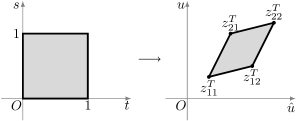
Figure 3: Illustration of the change of variables from the $(s,t)$- to the $(u,{\hat{u}})$-plane. We denote $z^{T}_{\mu\nu}=z_{\mu\nu}+Tu$, cf. (45).

So the integral we are interested in is

$$\int_{X}^{(m)}\!\mathrm{d}{s}\int_{Y}^{(n)}\!\mathrm{d}{t}\left(P_{1}(z_{c\pm};z_{1})+P_{2}(z_{c\pm};z_{1})\ln|z_{c\pm}|\right)$$ (52)

$$=\int_{0}^{1}\!\mathrm{d}{s}\int_{0}^{1}\!\mathrm{d}{t}\frac{(1-s)^{m}}{m!}\frac{(1-t)^{n}}{n!}\left(P_{1}(z_{c\pm};z_{1})+P_{2}(z_{c\pm};z_{1})\ln|z_{c\pm}|\right)$$ (53)

$$=\pm\int_{X\wedge Y}\frac{\left(1-\frac{y\wedge(z-z_{11})}{x\wedge y}\right)^{m}}{m!}\frac{\left(1-\frac{x\wedge(z-z_{11})}{x\wedge y}\right)^{n}}{n!}\left(P_{1}(z_{c\pm};z_{1})+P_{2}(z_{c\pm};z_{1})\ln|z_{c\pm}|\right)\frac{\mathrm{d}{z_{c\pm}}\wedge\mathrm{d}{z_{1}}}{x\wedge y}.$$ (54)

Since any 2-form is closed (being top dimensional) by the Poincaré lemma, it is also exact; i.e., we can write the differentials in (54) as $\mathrm{d}{Q}$ where $Q$ is some 1-form. Then by Stokes’s theorem, we can reduce the integral in (54) from an integral over the interior to an integral over the boundary of the parallelogram. The boundary of the $st$ integration domain is $(0,0)\stackrel{{\scriptstyle s}}{{\longrightarrow}}(1,0)\stackrel{{\scriptstyle t}}{{\longrightarrow}}(1,1)\stackrel{{\scriptstyle-s}}{{\longrightarrow}}(0,1)\stackrel{{\scriptstyle-t}}{{\longrightarrow}}(0,0)$. In terms of the $z$ integration domain, this becomes $z_{11}\stackrel{{\scriptstyle-x}}{{\longrightarrow}}z_{21}\stackrel{{\scriptstyle y}}{{\longrightarrow}}z_{22}\stackrel{{\scriptstyle x}}{{\longrightarrow}}z_{12}\stackrel{{\scriptstyle-y}}{{\longrightarrow}}z_{11}$. We can formalize this procedure as follows. We are to integrate an expression of the form $P=\mathrm{d}Q$ where $Q$ is some 1-form. If we pull $Q$ back to any line, say $x$, then $Q_{x}$ is also top dimensional and therefore closed. Thus, we can write $Q_{x}=\mathrm{d}L_{x}$ with $L_{x}$ a 0-form, so that

$$\int_{X\wedge Y}P =\int_{\partial(X\wedge Y)}Q$$ (55)

$$=\sum_{\mu,\nu=1,2}(-)^{\mu+\nu}[L_{y}(z_{\mu\nu})-L_{x}(z_{\mu\nu})],$$ (56)

where $L_{x}$ corresponds to integration over an edge parallel to $x$ and similarly for $L_{y}$. In short, by applying Stokes’s theorem, we reduced the two-dimensional integral over the interior of the parallelogram to one-dimensional integrals over the edges. Moreover, these one-dimensional integrals are reduced to a sum over their end points, which are the vertices of the original parallelogram.

To actually get $Q$ from $P$, which is just the integrand in Eq. (54), we simply perform the $z_{c\pm}$ integration. Under this operation, the structure of the expression does not change:

$$\int\mathrm{d}z_{c\pm}\,(P_{1}(z_{c\pm};z_{1})+P_{2}(z_{c\pm};z_{1})\ln|z_{c\pm}|)\\ =P_{3}(z_{c\pm};z_{1})+P_{4}(z_{c\pm};z_{1})\ln|z_{c\pm}|.$$ (57)

The reason is that the $P_{i}(z_{c\pm};z_{1})$ coefficients depend polynomially on $z_{c\pm}$. The integration can then be done by elementary methods. The structure of $L$, obtained from $Q$, will be more complicated. It is discussed in Sec. IV.2.4.

IV.2.3 Variable change for parallel line segments

As mentioned before, when the line segments are parallel, it is no longer possible to construct an invertible transformation between $(s,t)$ and $(z_{0},z_{1})$. This is easily seen from the fact that parallelogram on the right of Fig. 3 collapses to a segment. Unfortunately, also, starting with formulas for the nonparallel case and taking a limit produces many technical difficulties. We found that it is most convenient to treat the $s$ and $t$ integrals in the parallel case separately, as is discussed below.

The failure to invertibly transform from $(s,t)$ to $(z_{0},z_{1})$ coordinates indicates that we can write $z_{0}$, $z_{1}$, $z(s,t,c)^{2}$ or any function $F(z_{0},z_{1})$ as a function $F(\zeta(s,t))$ of some single affine-linear combination $\zeta(s,t)$ of $s,t$ with nonzero constants $\zeta_{s}=\mathrm{d}\zeta/\mathrm{d}{s}$ and $\zeta_{t}=\mathrm{d}\zeta/\mathrm{d}{t}$ . Each $s$ or $t$ integral can then be converted into a $\zeta$ integral. The iterated integrals are now handled recursively. Denote $\zeta=\zeta(s,t)$, $\zeta^{S}=\zeta(0,t)$, $\zeta^{T}=\zeta(s,0)$ and $\zeta^{ST}=\zeta(0,0)$ and define

$$F_{m,n} =\frac{F^{[m+n+2]}(\zeta)}{\zeta_{s}^{m+1}\zeta_{t}^{n+1}}+\sum_{k=0}^{m+n+2}p^{S}_{m,n;k}(s)\frac{F^{[k]}(\zeta^{S})}{\zeta_{t}^{n+1}}$$

$$\quad{}+\sum_{k=0}^{m+n+2}p^{T}_{m,n;k}(t)\frac{F^{[k]}(\zeta^{T})}{\zeta_{s}^{m+1}}$$

$$\quad{}+\sum_{k=0}^{m+n+2}p^{ST}_{m,n;k}(s,t)F^{[k]}(\zeta^{ST}),$$ (58)

where the $p$’s (to be defined below) are polynomials in their arguments, while $F_{m,n}=F_{m,n}(\zeta,s,t)$ and

$$\frac{\mathrm{d}}{\mathrm{d}\zeta}F^{[k+1]} =F^{[k]},$$ (59)

$$F^{[0]} =F(\zeta),$$

$$F_{-1,-1} =F(\zeta).$$

The structure of this expression is preserved under integrations with respect to $s$ and $t$, with only the $p$’s changing, if we define

$$\int_{0}\mathrm{d}{s}\,F_{m,n}=F_{m+1,n}\quad\text{and}\quad\int_{0}\mathrm{d}{t}\,F_{m,n}=F_{m,n+1}.$$ (60)

Setting $s=t=1$ in $F_{m,n}$ precisely yields $I^{mn}_{l}$ defined in Eq. (32) for a proper choice of $F(\zeta)$. This choice is just the result of the $c$ integration given in Eq. (42), with the replacements $z_{1}=z_{1}(\zeta)$ and $z_{c\pm}=z_{c\pm}(\zeta)$.

Note that the integration constants are chosen such that $F_{m,n}=0$ whenever either $s=0$ or $t=0$ for any $m\geq 0$ or $n\geq 0$. With the above initial conditions, the polynomial coefficients will satisfy the following recurrence relations:

$$p^{S}_{m+1,n;k}(s) =\int_{0}\mathrm{d}{s}\,p^{S}_{m,n;k}(s)-\frac{\delta_{k,m+1+n+2}}{\zeta_{s}^{m+2}},$$ (61)

$$p^{S}_{m,n+1;k}(s) =p^{S}_{m,n;k-1}(s),$$ (62)

$$p^{T}_{m,n+1;k}(t) =\int_{0}\mathrm{d}{t}\,p^{T}_{m,n;k}(t)-\frac{\delta_{k,m+n+1+2}}{\zeta_{t}^{n+2}},$$ (63)

$$p^{T}_{m+1,n;k}(t) =p^{T}_{m,n;k-1}(t),$$ (64)

$$p^{ST}_{m+1,n;k}(s,t) =\int_{0}\mathrm{d}{s}\,p^{ST}_{m,n;k}(s,t)-\frac{p^{T}_{m,n;k-1}(t)}{\zeta_{s}^{m+2}},$$ (65)

$$p^{ST}_{m,n+1;k}(s,t) =\int_{0}\mathrm{d}{t}\,p^{ST}_{m,n;k}(s,t)-\frac{p^{S}_{m,n;k-1}(s)}{\zeta_{t}^{n+2}}.$$ (66)

The coefficients that are relevant for the integrals we consider can be found in Table 2.

		$p$	$p^{S}$	$p^{T}$	$p^{ST}$
$m=0,n=0$	$k=2$	$\frac{1}{\zeta_{s}\zeta_{t}}$	$-\frac{1}{\zeta_{s}\zeta_{t}}$	$-\frac{1}{\zeta_{s}\zeta_{t}}$	$\frac{1}{\zeta_{s}\zeta_{t}}$
$m=1,n=0$	$k=2$		$-\frac{s}{\zeta_{s}\zeta_{t}}$		$\frac{s}{\zeta_{s}\zeta_{t}}$
	$k=3$	$\frac{1}{\zeta_{s}^{2}\zeta_{t}}$	$-\frac{1}{\zeta_{s}^{2}\zeta_{t}}$	$-\frac{1}{\zeta_{s}^{2}\zeta_{t}}$	$\frac{1}{\zeta_{s}^{2}\zeta_{t}}$
$m=0,n=1$	$k=2$			$-\frac{t}{\zeta_{s}\zeta_{t}}$	$\frac{t}{\zeta_{s}\zeta_{t}}$
	$k=3$	$\frac{1}{\zeta_{s}\zeta_{t}^{2}}$	$-\frac{1}{\zeta_{s}\zeta_{t}^{2}}$	$-\frac{1}{\zeta_{s}\zeta_{t}^{2}}$	$\frac{1}{\zeta_{s}\zeta_{t}^{2}}$
$m=1,n=1$	$k=2$				$\frac{st}{\zeta_{s}\zeta_{t}}$
	$k=3$		$-\frac{s}{\zeta_{s}\zeta_{t}^{2}}$	$-\frac{t}{\zeta_{s}^{2}\zeta_{t}}$	$\frac{s\zeta_{s}+t\zeta_{t}}{\zeta_{s}^{2}\zeta_{t}^{2}}$
	$k=4$	$\frac{1}{\zeta_{s}^{2}\zeta_{t}^{2}}$	$-\frac{1}{\zeta_{s}^{2}\zeta_{t}^{2}}$	$-\frac{1}{\zeta_{s}^{2}\zeta_{t}^{2}}$	$\frac{1}{\zeta_{s}^{2}\zeta_{t}^{2}}$

Table 2: The polynomial coefficients from Eq. (58) for the parallel case for different values of $m,n$ and $k$.

Thus, also for the parallel situation, we are left to evaluate one-dimensional integrals, in particular, integrals parametrized by $\zeta(s,t)$. Our calculations require two-, three- and maximally four-iterated integrals. One can think of these integrals in a similar way as for the integrals in the nonparallel situation: the $\zeta(s,t)$ parametrizes the sides of the parallelogram and the four terms in (58) correspond to the four edges of the parallelogram.

In sum, for both situations, nonparallel and parallel line segments, we are left to evaluate one-dimensional integrals along the sides of a parallelogram. Evaluation of these one-dimensional integrals is discussed next.

IV.2.4 Edge segment integrals

In the two preceding sections, we have converted the two-dimensional integrals over $s$ and $t$ into one-dimensional integrals over the boundary edges of the parallelogram on the right of Fig. 3. In the nonparallel case, these are the integrals on the right-hand side of Eq. (55). In the parallel case, these are the integrals that solve Eq. (59). In either case, we need to find a convenient way to parametrize the edge segments (we will use a parameter $\sigma$) and keep track of the structure of the integrand. We address this below.

We again need to consider two different situations: one in which the edge is completely in the direction of $u$ and one in which the edge also has a ${\hat{u}}$ component. A different parametrization is needed for each case. However, in both cases, each side of the parallelogram is described by its starting point $b$ and its tangent vector $a$, which runs from one vertex to the next. First the procedure for the latter situation, which corresponds to $a\cdot{\hat{u}}\neq 0$ is outlined and successively the situation in which the edge is entirely in the $u$ direction, that is, $a\cdot{\hat{u}}=0$.

Case $a\cdot{\hat{u}}\neq 0$.

When $a\cdot{\hat{u}}\neq 0$, we parametrize each edge by $z(\sigma)=z_{0}(\sigma)u+z_{1}(\sigma){\hat{u}}$ with

$$z_{0}(\sigma) =B_{0}-C_{0}\sigma,$$ (67)

$$z_{1}(\sigma) =\sigma.$$ (68)

To relate the constants $B_{0}$ and $C_{0}$ to the geometry of the parallelogram, we look at the “velocity” of the edge

$$\frac{\mathrm{d}}{\mathrm{d}{\sigma}}z(\sigma)=Ka,$$

where $K$ is an unknown constant. If we dot this equation with $-u$ and ${\hat{u}}$, we can compare this to the derivatives of $z_{0}$ and $z_{1}$ to determine $C_{0}$ in terms of the $a$ and $b$ vectors

$$\frac{-K(a\cdot u)}{K(a\cdot{\hat{u}})}=\frac{\frac{\mathrm{d}{z_{0}}(\sigma)}{\mathrm{d}{\sigma}}}{\frac{\mathrm{d}{z_{1}}(\sigma)}{\mathrm{d}{\sigma}}}=\frac{-C_{0}}{1}\Longrightarrow C_{0}=\frac{a\cdot u}{a\cdot{\hat{u}}}.$$

To determine $B_{0}$ in terms of the $a$ and $b$ vectors, we look at the starting point of the edge which corresponds to $\sigma=0$. At this point $z(\sigma=0)=b$, but also $z(\sigma=0)=z_{0}(0)u+z_{1}(0){\hat{u}}$, which upon applying $a\wedge u=(a\cdot{\hat{u}})\,({\hat{u}}\wedge u)=-a\cdot{\hat{u}}$ shows that $B_{0}=-\frac{a\wedge b}{a\cdot{\hat{u}}}$. After integration along the vertices, the start and end point of each segment needs to be inserted, which is at each vertex $\sigma=b\cdot\hat{u}$.

The ($z_{c\pm}$,$z_{1}$) variables are related to these new variables as follows. We already know that $z_{1}=\sigma$ and $z_{c\pm}$ is obtained by

$$z_{c\pm} =c+z_{1}\mp z_{0}$$ (69)

$$=c+\sigma\mp B_{0}\pm C_{0}\sigma$$ (70)

$$=B_{c\pm}\left(1-C_{c\pm}\sigma\right),$$ (71)

where we defined $B_{c\pm}=c\mp B_{0}$ and $C_{c\pm}=-\frac{1\pm C_{0}}{c\mp B_{0}}$. Hitherto, the shift in the $u$ direction from the temporal smearing [see Eqs. (35) and (36)] has not been explicitly taken into account. Fortunately, it can be simply re-obtained by absorbing the shift in the $b$ vector: $b\cdot u\to b\cdot u-T$. This gives

$$B_{0}=-\frac{a\wedge b}{a\cdot{\hat{u}}}\longrightarrow-\frac{a\wedge b}{a\cdot{\hat{u}}}+T.$$ (72)

$C_{0}$ does not change as it does not contain $b$. Thus, taking the shift by the smearing into account, we have

$$B_{c\pm} =\frac{(a\cdot{\hat{u}})(c\mp T)\pm a\wedge b}{a\cdot{\hat{u}}},$$ (73)

$$C_{c\pm} =-\frac{a_{\pm}}{a\cdot{\hat{u}}(c\mp T)\pm a\wedge b}.$$ (74)

For the parallel case, we identify $\zeta=\sigma$. The constants $\zeta_{s}$ and $\zeta_{t}$ can also be related to this setup: $\zeta_{s}=-x\cdot{\hat{u}}$ and $\zeta_{t}=y\cdot{\hat{u}}$.

Case $a\cdot{\hat{u}}=0$.

When $a\cdot{\hat{u}}=0$, a different parametrization of the edges is needed. This is simply done by reversing the role of $z_{0}$ and $z_{1}$

$$z_{0} =\sigma,$$ (75)

$$z_{1} =B_{0}-C_{0}\sigma.$$ (76)

With the same procedure as before, we obtain that in this parametrization $z_{c\pm}=B_{c\pm}\left(1-C_{c\pm}\sigma\right)$ remains the same, but the constants $B_{c\pm}$ and $C_{c\pm}$ change. Thus,

$$B_{0} =b\cdot\hat{u},\qquad B_{c\pm} =c+b\cdot\hat{u},$$ (77)

$$C_{0} =0,\qquad C_{c\pm} =\frac{\pm 1}{c+b\cdot\hat{u}},$$ (78)

and at the starting point of each edge $\sigma=-b\cdot u$. When the shift due to smearing is taken into account, $B_{c\pm}$ and $C_{c\pm}$ are not altered. In contrast, at each edge, $\sigma$ is shifted to $\sigma\to-b\cdot u+T$. For the parallel case, we again identify $\zeta=\sigma$ and the constants $\zeta_{s}$ and $\zeta_{t}$ in this setup are $\zeta_{s}=x\cdot u$ and $\zeta_{t}=-y\cdot u$.

The structure of the edge integrands after each edge is parametrized with the appropriate $\sigma$-parameter changes as follows (we use $\to$ instead of $=$ below because some terms proportional to $\ln|\sigma|$ are omitted from the result, as explained further on):

$$P_{3}+P_{4}\ln|z_{c\pm}| \to P_{5}+P_{6}\ln|B_{c\pm}|+P_{7}\ln|1-C_{c\pm}\sigma|$$

$$\quad{}+P_{8}\operatorname{L}(C_{c\pm}\sigma).$$ (79)

The $P_{i}(z_{c\pm};z_{1})$ coefficients are polynomial in $z_{c\pm}$ and Laurent polynomial in $z_{1}$. Their structure is taken from Eq. (57) in the nonparallel case and directly from Eq. (42) for the parallel case. The function $\operatorname{L}(x)$ is defined in terms of the dilogarithm dil (2013); Maximon (2003)

$$\operatorname{L}(x)=\operatorname{Re}\{\operatorname{Li}_{2}(x)\}=-\int_{0}^{x}\mathrm{d}{t}\,\frac{\ln|1-t|}{t}.$$ (80)

After the $\sigma$ substitution, the new coefficients are obviously Laurent polynomials in $\sigma$. In the $a\cdot{\hat{u}}=0$ case, they are just polynomial, since in that case $z_{1}$ is constant and hence independent of $\sigma$. As written, the coefficient $P_{8}=0$. However, its inclusion makes the structure of the expression on the right-hand side of (79) stable under $\sigma$ integration, which generically changes the value of $P_{8}$. In the nonparallel case, $\sigma$ integration need only be carried out once. But in the parallel case, it may need to be carried out repeatedly to generate the $F^{[k]}(\zeta)$ functions. It then becomes important to recognize the stability of the given expression structure.

The $\sigma$ integrals can be done using elementary means, with a partial exception for the $P_{7}$ and $P_{8}$ term. Recall that all the $P_{i}$ coefficients are rational, with poles only at $\sigma=0$. Thus, also the $P_{5}$ and $P_{6}$ terms are rational and hence have rational integrals, with the possible exception of terms proportional to $\ln|\sigma|$. They are omitted from the result for the following reason. The singularity of the integrand at $\sigma=0$ appears because of the presence of inverse powers of $z_{1}$ in the summand of Eq. (42). However, the corresponding original $c$ integral is regular at $z_{1}$ and thus all $z_{1}=0$ (and hence all subsequent $\sigma=0$) singularities must cancel in the final sum over the $\pm$ and $c=\pm R$ ranges. The same reasoning explains the exclusion of $b\cdot{\hat{u}}=0$ singularities as discussed in Sec. IV.2.5. The integral of the $P_{7}$ term has the same structure up to terms absorbed by $P_{5}$, with the exception of simple poles like

$$\int\mathrm{d}\sigma\,\frac{1}{\sigma}\ln|1-C_{c\pm}\sigma|=-\operatorname{L}(C_{c\pm}\sigma),$$ (81)

which obviously produce terms absorbed by $P_{8}$. Using integration by parts and the above identity, the $P_{8}$ term also produces an integral of the same form, up to terms absorbed into $P_{5}$ and $P_{7}$.

The final result for the integral $I^{mn}_{l}(R,T;X,Y)$ defined in Eq. (32) can be organized as follows. There are two possible expressions, one for the case when $X$ and $Y$ are not parallel and one for the case when they are. In either case, the expression has the structure of the sum over the values $c=\pm R$, over the $\pm$ indices carried by ($z_{c\pm}$, $B_{c\pm}$ and $C_{c\pm}$), as indicated in Eq. (42), and over the parallelogram vertices $z_{\mu\nu}$, as indicated in Eq. (56) (nonparallel case) or Eq. (58) (parallel case). The summand has the structure of the right-hand side of Eq. (79), with the $P_{i}$ coefficients computed according the procedure discussed above.

IV.2.5 Singularity structure

Recall that ultimately we are interested in obtaining an asymptotic expansion for small $\mu$, with leading behavior of the form $\mu^{i}\ln^{j}\mu$ for some $i$ and $j\geq 0$. For that, we do not need the full dependence of $I^{mn}_{l}(R,T;X,Y)$ on $R$ and $T$. We only need the leading-order expansion for $R,T\to 0$. A priori, it is not completely obvious what form this expansion will take. However, our explicit calculations show, based on Eq. (79), that it is possible to expand in products of powers of $S$, $\ln|S|$ and $\text{sgn}S=S/|S|$, where $S$ is $R$, or $R\pm T$. Note that the form of such an expansion is stable under differentiation with respect to $R$ or $T$, provided we supplement it with terms proportional to $\delta(S)$. Recall that such differentiations will be necessary in the evaluation of “part II” in Eq. (31), described in step 1 of Sec. IV.3. In this section, we describe how these expansions are carried out and tabulated for later lookup during the final smearing phase described in Sec. IV.3.

The $R,T$ expansion can be carried out mechanically with computer algebra using the following simple trick. We replace $R\to\epsilon R$, $T\to\epsilon T$, where $\epsilon$ is a symbolic parameter and expand in powers of $\epsilon$ and $\ln\epsilon$. After truncating at the desired order and setting $\epsilon\to 1$, for each term of the resulting expression, we use pattern matching to extract its structure (the $R,T$-independent coefficient, the value of $S$ and the powers in $S^{i}\ln^{j}|S|(\text{sgn}S)^{k}$). So, the result of each expansion is stored in structured form. Rational and logarithmic expressions can be efficiently expanded by Mathematica as they are. But the dilogarithm $\operatorname{L}(x)$ poses a few problems because of the need to select a specific branch at $x=\pm\infty$ and $x=1$. To circumvent this issue, if we expect to expand about these arguments, we first use one of the following identities Maximon (2003) and exploit the fact that $\operatorname{L}(x)$ is analytic at $x=0$:

$$\operatorname{L}(1/x) =-\operatorname{L}(x)-\frac{1}{2}\ln^{2}|x|+\frac{\pi^{2}}{12}+\frac{x}{|x|}\frac{\pi^{2}}{4},$$ (82)

$$\operatorname{L}(1-x) =-\operatorname{L}(x)-\ln|1-x|\ln|x|+\frac{\pi^{2}}{6}.$$ (83)

Consider the expression $\ln|A+BS|$. It can clearly have different leading $S\to 0$ behaviors (or singularity structure) depending on the values of the constants $A$ and $B$. For example, if $A\neq 0$, then it behaves like $\ln|A|+(B/A)S+\cdots$, while if $A=0$, it behaves like $\ln|S|+\ln|B|$. The same situation occurs for the expressions $I^{mn}_{l}(R,T;X,Y)$ depending on the relative geometry of the segments $X$ and $Y$. The geometry of these segments is captured by the geometry of the parallelogram illustrated in Fig. 3. As discussed at the end of the preceding section (Sec. IV.2.4), the expression to be expanded consists of a sum of many terms, each of which depends only on a given pair of vectors $a$ and $b$ in the $(u,{\hat{u}})$-plane, where $b$ is a parallelogram vertex (one of the $z_{\mu\nu}$) and $a$ is one of the incident parallelogram edges ($\pm x$ or $\pm y$), cf. Fig. 4. The actual dependence appears a functional dependence on the possible geometric scalars generated from the vectors $a$, $b$, $u$ and ${\hat{u}}$: $a\cdot b$, $a\wedge b$, $a^{2}$, $b^{2}$, $a_{\pm}$, $b_{\pm}$, $a\cdot u$, $a\cdot{\hat{u}}$, $b\cdot u$, $b\cdot\hat{u}$. Not all of these scalars are independent, so for the purposes of some symbolic manipulations they are expressed in terms of a convenient independent subset.

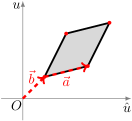
Figure 4: Illustration of the role of the vectors $a$ and $b$ defined in the text. The vertices of the parallelogram are $z_{\mu\nu}$ and each side is a multiple of either $x$ or $y$, defined in Eq. (45).

Each end point of the $X$ and $Y$ gives rise to a light cone. Given the nature of the original integrand (the Hadamard two-point function) in the definition of $I^{mn}_{l}(R,T;X,Y)$, it is not surprising that its singularity structure depends on the position of one segment with respect to the light cones generated by the other segment or itself. A detailed study of the expressions in Eq. (79) essentially confirms this expectation. Although, there also appear other considerations that stem from our particular choices in parametrizing the edge segment integrals, as described in Sec. IV.2.4. The detailed decision trees for determining the singularity structure for nonparallel and parallel cases are illustrated in Fig. 5. For each possible singularity type, a subset of the scalars listed in the preceding paragraph is consistently set to zero, and the $R,T$ expansion is carried out mechanically (as described before) and the result is stored in structured form in the indicated table.

After the remaining $R,T$ smearing of “part II”, the final answer for $\langle\tilde{r}^{2}\rangle$ is expected to be of order $1/\mu^{2}$. We would like to compute a few subleading terms as well, namely up to and including terms of order $\mathcal{O}(\mu^{0})$. Since the $R,T$ smearing involves applying up to two derivatives before integrating with respect to the smearing profile, we must expand in $R$ and $T$ and keep terms up to and including order $\mathcal{O}(R,T)^{2}$. However, if we are expanding $I^{mn}_{l}$ with $l>0$, which contained $c^{l}$ in the original integrand, we must keep terms up to and including order $\mathcal{O}(R,T)^{2+l}$, because the definition of $c$ given in Sec. IV.1.1 contains an implicit power of $R$.

As discussed above, the coefficients of the $R,T$ expansion are functions of various geometric scalars formed from the vectors $a$, $b$, $u$ and ${\hat{u}}$, and in particular $b\cdot\hat{u}$. Some of them contain terms like $(b\cdot\hat{u})\ln b\cdot\hat{u}$, which have well-defined, finite values at $b\cdot\hat{u}=0$. Unfortunately, direct evaluation of such expressions at $b\cdot\hat{u}=0$ by Mathematica produces errors. We have circumvented this problem by taking the $b\cdot\hat{u}\to 0$ limit symbolically beforehand. In the parallel case, the limit is taken on fully symbolic expressions and is tabulated separately. However, the same strategy proved to be prohibitively expensive, with our computational resources, in the nonparallel case, due to the complexity of the fully symbolic expressions inside the limit. Instead, we take the limit at a later point of the calculation, when the numerical values of all the geometric scalars are available. All of their numerical values are substituted into the tabulated expression, with the exception of $b\cdot\hat{u}$, and the symbolic limit is taken.

We finish this subsection by briefly summarizing the decision logic illustrated in Fig. 5. We start with an exact formula for the summand giving $I^{mn}_{l}(R,T;X,Y)$ for nonparallel or parallel segments, as in Secs. IV.2.2 and IV.2.3. Then, we check $a\cdot{\hat{u}}=0$, which decides the edge segment parametrization to be used, as in Sec. IV.2.4. In the nonparallel case, the $a\cdot{\hat{u}}=0$ is trivial, since the integrand is proportional to $\mathrm{d}{z_{1}}$, which vanishes in this case. In the parallel case, we further implicitly assume that $a\cdot u\neq 0$, since otherwise $a=0$, a case that we do not consider. Next, we check whether $a_{\pm}\neq 0$ (in our code labeled ‘generic’) or $a_{\pm}=0$ (in our code labeled ‘special’). Recall that one of $a_{+}$ or $a_{-}$ vanishes precisely when $a$ lies on one or the other branch of the light cone in the $(u,{\hat{u}})$-plane. Finally, we check the condition $b\cdot\hat{u}=0$. The decision trees in Fig. 5 show which table stores the values of the expansion of $I^{mn}_{l}(R,T;X,Y)$ with the needed singularity structure. Each table is indexed by the integers $m,n$ (numbers of iterated segment integrals) and $l$ (power of $c^{l}$).

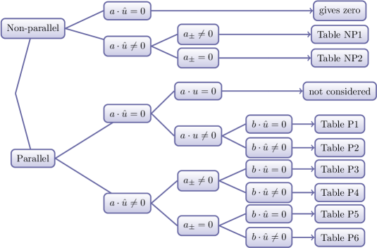
Figure 5: Decision tree summarizing the procedure for the nonparallel and parallel cases.

IV.3 Remaining smearing

Recall the master formula (31) for $\tilde{I}^{mn}_{K}(X,Y)$. As described in the preceding sections, ‘part I’ of the calculation has been computed exactly as $I^{mn}_{l}(R,T;X,Y)$, expanded for small $R$ and $T$ and an appropriate truncation of the expansion has been stored in a look-up table. The truncated expansion is of the form

$$I^{mn}_{l}(R,T;X,Y)\sim\sum_{f}I^{mn}_{l,f}(X,Y)f(R,T),$$ (84)

where each $f(R,T)$ is a product of (possibly singular) powers of $R$, $R\pm T$, $\ln|R\pm T|$ or $\text{sgn}(R\pm T)$. For simplicity of notation, we do not show the structure of the truncated expansions in more detail. The evaluation of ‘part II’ is carried out algorithmically with the following steps, which correspond roughly to the summation over the indices $d$, $\gamma$, $p$ and finally $l$:

1. The summation over $l$ may be carried at any time, so we do it first.

2. The $T$ integrals are evaluated by moving all $T$ derivatives from $\delta^{(d)}(-T)$ onto the $f(R,T)$ using integration by parts and effecting the replacement $T\to 0$. The $\text{sgn}(R\pm T)$ terms generate $\delta(R)$’s or derivatives thereof.

   At this point, the summation over $d$ may be carried out.

3. Terms proportional to $\delta(R)$ and its derivatives are also evaluated using integration by parts and by effecting the replacement $R\to 0$. This part of the calculation is then stored separately. It may contain terms proportional to $g^{(\gamma)}(0)$.

4. In the remaining terms, each $f(R,T)$ has by now been transformed into a linear combination of terms of the form $g^{(\gamma)}(R^{2})R^{i}\ln^{j}R$ with powers $i$ such that all integrals are convergent near $R=0$. Formal integration by parts (which neglects the boundary terms at $R=0$) can bring this expression to the form where each term is now $g(R^{2})R^{i}\ln^{j}R$. However, the powers $i$ may now take values for which the integrals diverge near $R=0$. They are to be interpreted as distributional integrals, defined by the Hadamard finite part regularization.

   At this point, the summation over $\gamma$ may be carried out.

5. The distributional $R$ integrals are replaced by moments of the smearing function according to the rule

   $$\int_{0}^{\infty}\mathrm{d}{R}\,g(R^{2})\,R^{i}\ln^{j}R=\mu^{i-2}_{(i,j)}\ln^{j}|\bar{\mu}_{(i,j)}|,$$ (85)

   where the numbers $\mu_{(i,j)}$ and $\bar{\mu}_{(i,j)}$ parametrize the moments. For simplicity we simply set $\bar{\mu}_{(i,j)}=\mu_{(i,j)}=\mu$.

   At this point, the summation over $p$ may be transformed into the summation over $i$ in (31).

Once the coefficients $P_{\mathsf{T},d,\gamma,p,l}$ and the truncated expansions of $I^{mn}_{l}(R,T;X,Y)$ are known, all of the above operations involve only elementary algebra on moderate sized expressions and thus can be efficiently carried out on demand. The result is an expression for $\tilde{I}^{mn}_{K}(X,Y)$ in the form given on the last line of Eq. (31). In practice, we truncate the expansions so that the coefficients $I^{mn}_{\mathsf{T},i}(\ln\mu;X,Y)$ are known for $i=0,1$ and $2$. A few comments about some of the above steps are in order.

Note that the values $g^{(\gamma)}(0)$, possibly obtained in step 2, can also be seen as moments of the smearing function, though different from those defined in Eq. (85). In terms of rough scaling, we expect $g^{(\gamma)}(0)\sim\mu^{-3-2\gamma}$. Thus, the appearance of a $g(0)$ in the result of the calculation would signify a more singular leading-order term ($\sim\mu^{-3}$) than is expected by dimensional analysis and by the form of the last line of (31). Such terms do actually occur in the calculation. Fortunately, and as is to be expected, they ultimately cancel in the summation over the $X,Y$ segments in Eq. (96). This cancellation is taken to be part of the consistency check on our calculation (Sec. V.1).

The use of formal integration by parts and the Hadamard finite part regularization in step 3 are linked. Hadamard finite part (also partie finie) regularization (Gelʹfand and Shilov, 1964, Ch.I§3) is defined for singular integrands $f(R)$ that vanish in the neighborhood of $R=\infty$ and for which there exists a bivariate polynomial $A(x,y)$ such that the following limit is finite:

$$P.f.\int_{0}^{\infty}f(R)\,\mathrm{d}{R}=\lim_{\epsilon\to 0^{+}}\int_{\epsilon}^{\infty}f(R)\,\mathrm{d}{R}-A(\epsilon^{-1},\ln\epsilon).$$ (86)

The polynomial $A$ is unique up to the addition of a constant, which may be absorbed by the replacement $\ln\epsilon\to\ln\epsilon/C$. This constant may be fixed by requiring that $P.f.\int_{0}^{\infty}f^{\prime}(R)\,\mathrm{d}{R}=-f(0)$ is always true, provided $f(r)$ vanishes at $R=\infty$. If the $R$ integrals in “part II” are treated from the start as distributional integrals Gelʹfand and Shilov (1964), with the differentiated smearing functions $g^{(\gamma)}(R^{2})$ playing the role of test functions, then the formal application of integration by parts produces precisely distributions regularized according to the Hadamard finite part prescription . The only addition to formal integration by parts necessary for the above statement to hold is the rule $1\cdot\frac{\mathrm{d}}{\mathrm{d}{R}}f(R)\to-\delta(R)f(R)$, rather than $0$. This extra boundary term is then handled the same as in step 2.

IV.4 Updated master formula for $\langle\tilde{r}^{2}\rangle$

It remains now to evaluate the sums and tensor contractions in the master formula (19) for $\langle\tilde{r}^{2}\rangle$. The tensor contractions consist of evaluating expressions of the form

$$r^{Kij}_{nX}\eta_{ij,kl}r^{Lkl}_{mY}\mathsf{T}_{K\cup L},$$ (87)

where $|K|,|L|=0$ or $1$. Reading off the tensorial coefficients from the explicit expression for $r[h]$, Eq. (4), we can write them in factored form

$$r^{Kij}_{nX}=x^{i}A^{Kj}_{nX},$$ (88)

where $x$ is the vector corresponding to the segment $X$, with the orientation indicated by Fig. 8. For any tensor basis element $\mathsf{T}$, we can define the contraction

$$E_{\mathsf{T},mn}^{jl}(X,Y)=\sum_{K,L}(-)^{|L|}A^{Kj}_{nX}\mathsf{T}_{K\cup L}A^{Ll}_{mX},$$ (89)

with the convention that $\mathsf{T}_{J}=0$ for any multi-index $J$ whose size $|J|$ does not equal the tensor rank of $\mathsf{T}$. We show the structure of the above multi-index sums explicitly for the needed tensor ranks. Let $\mathsf{T}^{p}$ stand for a tensor basis element of rank $p$ (recall also that $\mathsf{T}^{0}$ takes only one value, the scalar $1$):

$$E_{\mathsf{T}^{0},mn}^{jl}(X,Y) =A^{j}_{mX}A^{l}_{nY},$$ (90)

$$E_{\mathsf{T}^{1},mn}^{jl}(X,Y) =-A^{j}_{mX}\mathsf{T}^{1}_{l_{1}}A^{l_{1}\,l}_{nY}+A^{k_{1}\,j}_{mX}\mathsf{T}^{1}_{k_{1}}A^{l}_{nY},$$ (91)

$$E_{\mathsf{T}^{2},mn}^{jl}(X,Y) =-A^{k_{1}\,j}_{mX}\mathsf{T}^{2}_{k_{1}l_{1}}A^{l_{1}\,l}_{nY}.$$ (92)

The remaining tensor contraction is evaluated using the formula for $\eta_{ij,kl}$ from Eq. (13):

$$\eta_{ij,kl}\,x^{i}y^{k}E^{jl}=(x\cdot y)\operatorname{tr}E+E(y,x)-E(x,y),$$ (93)

where $\operatorname{tr}E=\eta_{jl}E^{jl}$ and $E(a,b)=E^{jl}a_{j}b_{l}$. The updated master formula for the quantum variance $\langle\tilde{r}^{2}\rangle$, combining Eqs. (19) and (31), can now be written as follows:

$$\langle\tilde{r}^{2}\rangle =\frac{\ell_{p}^{2}}{2\pi}\sum_{KmX}\sum_{LnY}(-)^{|L|}r^{Kij}_{mX}\,\eta_{ij,kl}\,r^{Lkl}_{nY}\,\frac{2\pi}{\mu^{2}}\sum_{q=0}^{\infty}\sum_{\mathsf{T}}\mathsf{T}_{K\cup L}\,\mu^{q}\,I^{mn}_{\mathsf{T},q}(\ln\mu;X,Y),$$ (94)

$$=\frac{\ell_{p}^{2}}{\mu^{2}}\sum_{mX}\sum_{nY}\sum_{q=0}^{\infty}\sum_{\mathsf{T}}\mu^{q}\,\eta_{ij,kl}\,x^{i}y^{k}\,E_{\mathsf{T},mn}^{jl}(X,Y)\,I^{mn}_{\mathsf{T},q}(\ln\mu;X,Y)$$ (95)

$$=\frac{\ell_{p}^{2}}{\mu^{2}}\sum_{q=0}^{\infty}\mu^{q}\sum_{X}\sum_{Y}\eta_{ij,kl}\,x^{i}y^{k}\sum_{m,n}\sum_{\mathsf{T}}E_{\mathsf{T},mn}^{jl}(X,Y)\,I^{mn}_{\mathsf{T},q}(\ln\mu;X,Y).$$ (96)

Notice, from the above formula, that the final result for $\langle\tilde{r}^{2}\rangle$ may depend on powers of $\mu$ as well of $\ln\mu$. However, it will be seen in the next section that $\ln\mu$ does not actually appear in the final result. This fortuitous cancellation can be seen as an explicit verification of the simple dimensional analysis yielding the $1/\mu^{2}$ leading singular behavior, as well as a check on the correctness of our calculations (Sec. V.1).

This last formula (96), directly forms the basis of our computer algorithm for explicitly evaluating $\langle\tilde{r}^{2}\rangle$ for a fixed geodesic triangle geometry. We briefly summarize the logic:

1. Load lookup tables for the tensor coefficients $A^{Ki}_{mX}$ [Eqs. (4) and (88)], tensor basis elements $\mathsf{T}$ and polynomial coefficients $P_{\mathsf{T},d,\gamma,p,l}$ [Eq. (28) and Table 1], and truncated expansions for $I^{mn}_{l}(R,T;X,Y)$ [Sec. IV.2, Eq. (32), Fig. 5].

2. Construct the segments $X$ of the geodesic triangle geometry as in Fig. (8).

3. For fixed $m,X,n,Y$ and $\mathsf{T}$, compute the coefficients $I^{mn}_{\mathsf{T},q}(\ln\mu;X,Y)$ [Eq. (31) and Sec. IV.3] and the matrix $E_{\mathsf{T},mn}^{jl}(X,Y)$ [Eqs. (89)–(92)].

4. Sum over $m$, $n$ and $\mathsf{T}$ in Eq. (96) and perform the remaining tensor contractions using Eq. (93).

5. Obtain $\langle\tilde{r}^{2}\rangle$ by summing over geodesic triangle geometry segments $X$ and $Y$ in Eq. (96) and keeping as many orders in $\mu^{q}$ as available or desired.

The results of explicit computations using the above algorithm are discussed in the next section.

V Results

Here we present the results of our calculation for the leading-order quantum gravitational corrections to the quantum variance of the emission time $\tau(s)$ regularized by a finite measurement resolution scale $\mu$ .

The experimental geometry is completely determined by two parameters: the reception time $s$ and the relative velocity $v_{rel}$ between the worldlines of the lab and the probe, which can also be parametrized by the (positive) hyperbolic rapidity $\theta$, with $v_{rel}/c=\tanh(\theta)$. Given these two inputs, in our approximation, Eqs. (6)–(8), the quantum mean and the variance of quantum fluctuations in the emission time are given by the following expressions

$$\langle\tilde{\tau}(s)\rangle =\tau_{\mathrm{cl}}(s)+\mathcal{O}(\ell_{p}^{2}),$$ (97)

$$(\Delta\tau)^{2} =\tau_{\mathrm{cl}}^{2}(s)\,\langle\tilde{r}^{2}\rangle+\mathcal{O}(\ell_{p}^{2}),$$ (98)

where, following Eq. (126),

$$\tau_{\mathrm{cl}}(s)=se^{-\theta}=s\,\sqrt{\frac{1-\frac{v_{rel}}{c}}{1+\frac{v_{rel}}{c}}}$$ (99)

and $\langle\tilde{r}^{2}\rangle$ is computed by the computer routine as described in Sec. IV.

Using dimensional analysis, as in Sec. III.1, we can parametrize the leading contributions to this expectation value as

$$\langle\tilde{r}^{2}\rangle=\frac{\ell_{p}^{2}}{\mu^{2}}\left(\rho_{0}+\rho_{1}\frac{\mu}{s}+\rho_{2}\frac{\mu^{2}}{s^{2}}+\mathcal{O}\left(\frac{\mu^{3}}{s^{3}}\right)\right)+\mathcal{O}\left(\frac{\ell_{p}^{2}}{\mu^{2}}\right),$$ (100)

where the $\rho_{i}$ coefficients are in general functions of $v_{rel}/c$. Note that the result is given to order $\mathcal{O}(\ell_{p}^{2}/\mu^{2})$ as we did not include the $\mathcal{O}(h^{2})$ term $\tilde{r}_{2}(h)$ in our calculation of the variance (see Sec. II.3). The explicit result of our computer calculation gives

$$\rho_{0} =\frac{1}{v^{2}}\left(\frac{51}{8}+8v+\frac{141}{8}v^{2}\right)$$ (101)

$$\quad{}-\frac{1}{v^{2}}\left(3+4v\right)\frac{(1-v^{2})}{v}\ln\left(\frac{1+v}{1-v}\right),$$

$$\rho_{1} =-2\pi^{2},$$ (102)

$$\rho_{2} =0.$$ (103)

The limiting value at $v=v_{rel}/c<1$ is $\rho_{0}=32$. These expressions are the main result of our calculation and were, in fact, the main motivation for it. They deserve a few comments.

It should be mentioned that, in addition to powers of $\mu$ as in Eq. (100), terms depending on $\ln\mu$ appeared in intermediate contributions to $\langle\tilde{r}^{2}\rangle$. Remarkably, they all canceled, so that the final expressions for $\rho_{i}$ given above depends only on powers of $\mu$. The components of the vectors representing the worldline segments $U$, $V$ and $W$ (Fig. 8) are rational functions of $v_{rel}/c$ and $s$. Rational expressions in these components appear as arguments of the graviton Hadamard two-point function and integrals thereof, as seen Sec. IV, which generate further rational and logarithmic expressions. It is therefore not surprising to see the $\rho_{i}$ coefficients of that form, with the $s$ dependence parametrized away in Eq. (100). However, their simplicity is striking. Note also that the dependence on $\pi$ is due only to dilogarithm identities Eqs. (82)–(83), since the overall factor $\frac{1}{2\pi}$ in (19) is absorbed into the normalization factor in the azimuthal angular averaging, Eqs. (29) and (30).

All the physically relevant information can be glimpsed from the low velocity approximation for the root-mean-square size of the quantum fluctuations

$$\Delta\tau\sim\sqrt{\frac{3}{8}}\left(\frac{c}{v_{rel}}\frac{s}{\mu}\right)\ell_{p}.$$ (104)

The dimensional scale of the effect is set by the Planck length, ($\ell_{p}\sim 10^{-35}\,\text{m}\sim 10^{-44}\,\text{s}$). There are two enhancement factors: the ratio $s/\mu$ of the experimental geometry and detector resolution scales, and the ratio $c/v_{rel}$ of the speed of light to the lab-probe relative velocity. We roughly estimated this enhancement factor in laboratory and cosmological experimental settings in Table 3. The large enhancement factors in the cosmological setting should be taken with a grain of salt. Foremost, curvature corrections must be added to our Minkowski calculation. Moreover, in either setting, the divergence of the enhancement factor for low velocities is rather puzzling, which we discuss next.

Table 3: The enhancement factor $(\frac{c}{v_{rel}}\frac{s}{\mu})$ for $\Delta\tau$, Eq. 104, over the Planck scale $\ell_{p}\sim 10^{-44}\,\text{s}$. Detector resolution scale: $\mu=10^{-9}\,\text{m}$ (X-ray wavelength). Laboratory scales: $s=1\,\text{m}$, $v_{rel}=1\,\text{m/s}$. Cosmological scales: $s=1\,\text{Mpc}\sim 10^{22}\,\text{m}$, $v_{rel}=10^{5}\,\text{m/s}$ (Hubble recession velocity at $1\,\text{Mpc}$), $v_{rel}=c/3\sim 10^{8}\,\text{m/s}$ (relativistic velocity).

	$v_{rel}$
$s$	$1\,\text{m/s}$	$10^{5}\,\text{m/s}$	$10^{8}\,\text{m/s}$
$1\,\text{m}$	$10^{17}$	$10^{12}$	$10^{9}$
$1\,\text{Mpc}$	$10^{39}$	$10^{34}$	$10^{31}$

A plot of the coefficient $\rho_{0}$ versus $v=v_{rel}/c$ is shown in Fig. 6. As is clear from the graph, $\rho_{0}$ diverges as $1/v^{2}$ in the limit $v\to 0$. It reaches a minimum around $v\sim 1/2$ and climbs to the limiting value of $\rho_{0}=32$ as $v\to 1$. The $\rho_{0}\sim 1/v^{2}$ divergence as $v\to 0$ is somewhat puzzling. The exponent of the divergence can be traced to the value of the normalization factor $\tau_{\mathrm{cl}}(s)(v\cdot w)$ [Eq. (135)] that appears in the denominator of the explicit expression for $r[h]$, Eq. (134). Classically, the integrals in the numerator of Eq. (134) all cancel so that $r[h]$ remains finite and in fact goes to $0$ as $v\to 0$. Afterall, there is no time delay if the lab and probe trajectories coincide. On the other hand, it seems that the quantum variance of the numerator in Eq. (134) goes to a nonzero constant as $v\to 0$, thus resulting in the divergence. While this result is interesting, the extrapolation of our calculation to $v\to 0$ must be taken with a grain of salt, since this limit violates our assumption that all sides of the geodesic triangle must be of size $s$ and that $\mu/s\ll 1$. We cannot exclude the possibility that the low velocity divergence is naturally regulated to a finite limit over the range $[0,\mu/s]$ of $v$ in a more accurate calculation. (The numerical values presented in Table 3 fall outside these transitional regions as there the critical velocity is $\mu/s\leq 0.1\,\text{m/s}$.) It is worth remarking that the dependence of $\rho_{0}$ on $v_{rel}$ could still be significantly altered by two factors: a different (hopefully Lorentz invariant) smearing procedure, and the inclusion of the quadratic correction $r_{2}[h]$ to the emission time, both of which would contribute corrections to the quantum variance at the order $\mathcal{O}(\ell_{p}^{2}/\mu^{2})$.

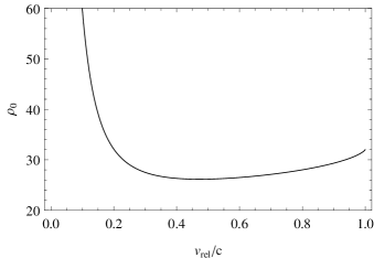
Figure 6: Plot of $\rho_{0}$ versus $v_{rel}/c$ for $\mu=1$. Note the divergence at $v_{rel}/c=0$, as discussed in the text.

Furthermore, a short note on the analytical formula (101). The computer calculation was carried out symbolically, but with fixed (rational) numerical values of $v=v_{rel}/c$ supplied as input. The analytical expression in terms of $v$ was obtained by a perfect fit to over 100 data points.

Finally, a comment on the calculation time. The calculation time can be divided into two parts (essentially “part I” and “part II” in Sec. IV): generating the tables (which only needs to be done once) and the explicit calculation of $\langle\tilde{r}^{2}\rangle$ for a given value of $v$. On a standard computer (AMD 64 Dual Core 2 GHz Processor) the first part takes approximately 45 minutes (once) and the second part takes about 20 minutes (per value of $v$). The most time consuming part in this latter calculation is the expansion in $b\cdot\hat{u}$ for nonparallel line segments. If this expansion could also have been tabulated, the calculation time for $\langle\tilde{r}^{2}\rangle$ would be drastically reduced.

V.1 Checks on results

We implemented several checks to make sure that we can be confident that the result presented is correct. First of all, the variance of any physical observable needs to be positive. It is obvious from the graph in Fig. 6 that $\langle\tilde{r}^{2}\rangle$ is always positive and this serves as a first check on our result. In addition, as was remarked in Appendix B, parts of the expression of $r$, viz. $H$ and $J$ of Eq. (134), are independently invariant under linearized diffeomorphism. These parts turn out to satisfy all other constraints on observables as well and are thus strictly speaking also observables, although their physical interpretation is not directly clear. Thus, $H^{2}$ and $J^{2}$ and any positive functional thereof should also be equal to or larger than zero. This was checked by the same routine that was used to calculate $\langle\tilde{r}^{2}\rangle$ and indeed it was shown that $\langle H^{2}\rangle\geq 0$ and $\langle J^{2}\rangle\geq 0$.

Second, the results nicely match the predictions made by a simple dimensional analysis: no terms more divergent than $1/\mu^{2}$ appear. In Khavkine (2012), it was noted that detailed calculations reveal terms with a more divergent scaling behavior (these terms are of the form $(\ell_{p}^{2}/\mu^{2})\ln\mu/s$ and $s\ell_{p}^{2}/\mu^{3}$); however, these terms cancel in the final result. A generic set of coefficients combining the $I^{mn}_{\mathsf{T},i}(\ln\mu;X,Y)$ in a sum over the $X$ and $Y$ segments would not result in a cancellation of the logarithmic terms. Thus it is unlikely that the cancellation would happen by accident (i.e., in the case of a programming error). This observation increases our confidence in the result, even if the cancellation of the logarithmic terms was not obvious in advance.

Third, there are two independent parts in our calculation where we expected intermediate results in the integrals to cancel each other in the final summations. One of these expected cancellations was (already mentioned in Sec. IV.2.1 and its reasoning further expanded upon in Sec. IV.2.4): the cancellation of terms singular in $z_{1}=0$ after all summations are taken into account. These terms singular in $z_{1}$ correspond to poles for $b\cdot\hat{u}=0$ after parametrization. In an independent routine we expanded the results from the integration in $b\cdot\hat{u}$ and checked whether we had rightfully thrown away all the lower-order terms: the outcome was positive, all lower-order terms vanish in the final summations over the overall $\pm$-sign, $c=\pm R$ and the four vertices . The other part where we expected cancellations to happen was related to the integration over $c$. This integration may produce terms that have the ‘wrong’ powers of $R$, which would eventually lead to terms scaling as $1/\mu^{4}$. Fortunately, these terms vanish when the boundaries of the $c$-summation are taken into account (so the summation over the $\pm$-sign and $c=\pm R$ is performed).

Fourth, as a check on the internal consistency of the routine that handles all integration by parts, the boundary terms produced by removing all derivatives from the smearing function nicely cancel with divergent terms in the bulk. This check is discussed in detail at the end of Sec. IV.3.

Lastly, the integral $\tilde{I}^{mn}_{K}(X,Y)$ has been calculated by hand for a simple case: $m=n=0$ (hence no iterated integrals) and along two parallel null segments. This has been done for zero, one as well as two derivatives on the smearing function, that is, $|K|=0,1,2$. The results of the calculation by hand match exactly the result produced by the computer routine and can be found in Appendix D.

All in all, these partial checks of various aspects of the calculation make us confident that the result presented is correct.

VI Discussion

In this paper, we have presented the first detailed calculation of the finite, measurement resolution regulated, quantum fluctuations in a gauge invariant, nonlocal, operationally defined observable in the Minkowski linearized quantum gravitational vacuum. As discussed in the Introduction, this is at least a partial improvement on previous works in a similar direction Ford (1995); Yu and Ford (1999); Borgman and Ford (2004); Thompson and Ford (2006); Woodard (1984); Tsamis and Woodard (1992); Ohlmeyer (1997); Roura and Arteaga . Unfortunately, this calculation is not yet the final word on the matter, due to some imperfect pragmatic technical choices made along the way. These will be recalled in more detail below. Still, our calculation can be seen as a very detailed template for a future, improved calculation or for generalizations, some examples of which are also discussed below.

The observable we considered is the time delay, induced by metric fluctuations, between proper time clocks moving at a predetermined relative velocity and compared using light signals. Generically speaking, this simple thought experiment setup can be seen as an idealization of possible laboratory scale, space based, or even cosmological scenarios. In each of these cases, our results, presented in Sec. V, give an estimate for the size of the quantum fluctuations and its dependence on the relative velocity of the clocks. Since this estimate is based only on the rather conservative model of linearized quantum gravity Burgess (2004), it can be used for several purposes. For instance, the expected size of the fluctuations can be compared to other sources of noise, like measurement uncertainties and even intrinsic quantum fluctuations in the measurement equipment, to see if it is reasonable to expect noticeable quantum gravitational effects in a given experimental setup. Unfortunately, in the scenarios we have considered, the quantum gravitational effects seem well below experimental sensitivity. However, it is not out of the question that alternative laboratory scenarios Wang et al. (2012) could bring the size of such effects closer to the current or future state of the art. Also, our estimate can be used to contrast predictions of the conservative linearized gravity model with more exotic “quantum gravity” models, which sometimes (so far unsuccessfully) lay claim to explain anomalies in cosmological observations, such as the dispersion in the arrival time of distant $\gamma$-ray burst photons Abdo et al. (2009); Amelino-Camelia et al. (1998); Hossenfelder and Smolin (2010).

Our result for the quantum fluctuation in the time delay shows two odd features, at least superficially: it is not Lorentz invariant and it diverges for low relative velocities. It fails to be Lorentz invariant because it selects a preferred relative velocity (where the fluctuations are at a minimum) between the two moving clocks (the lab and the probe). This phenomenon is mostly likely due to an explicitly non-Lorentz invariant choice of spacetime smearing applied to the graviton field. This smearing is physically significant, as it is interpreted as the cumulative effect of the intrinsic (quantum and statistical) fluctuations in the center of mass coordinates and the limited spacetime resolution of the measurement equipment. However, to make the calculation tractable, a pragmatic choice has been made to smear always in the lab’s spatial plane. While this is perfectly acceptable on the lab worldline, a future follow-up calculation should select a more realistic smearing profile for the probe and signal worldlines, preferably in a way that depends only on the local geometry of each worldline. The divergence in the size of the quantum fluctuations for small relative velocities, $v_{rel}\to 0$, on the other hand, is more puzzling. It is not clear what the physical interpretation of this result would be compatible with the fact that we do not observe such unbounded fluctuations in the everyday world of slowly relatively moving macroscopic objects. There are two chief possibilities that could explain it as an artifact of our particular calculation. One possibility is our approximation scheme. It treats the smearing length scale $\mu$ to be much smaller than the length scale $s$ related to the geometric scale of the experiment. But, as the relative velocity shrinks to zero, the size $\sim v_{rel}s$ of the signal worldline shrinks as well, eventually violating the $\mu\ll v_{rel}s$ requirement. Thus, it is possible that the divergence is resolved into a smooth transition to a finite limit, which unfortunately cannot be resolved within our approximation. The other possibility is that the inclusion of a quadratic correction to the perturbative formula for the time delay could cancel the low velocity divergence, since that term would contribute at the same order in $\ell_{p}/\mu$ as the result computed here. Its exclusion was again a pragmatic choice made to render the calculation tractable. A start was made in Appendix A, where the geodesic and parallel transport equation were calculated to second order in the gravitational field. These terms are to be included to get an expression for the time delay that is truly of quadratic order. However, presently, the computer routine is not able to handle some of these terms either because of the appearance of three derivatives acting on the graviton field (the code handles maximally two) or integration over the individual geodesic segments is not of a type that we considered (the $st$ integral is not over the whole unit square, but over the $0<s<t<1$ triangle). These terms should be fully taken into account in a follow-up calculation.

Despite the above drawbacks, we believe that the calculation and the result presented in this work constitute a valuable exercise in the treatment of phenomenologically meaningful, gauge invariant observables in quantum gravity. In particular, this calculation and the tools developed for it can be straightforwardly generalized to handle a large class of observables that in Khavkine (2012) were named quantum astrometric observables. This class includes the time delay, angular blurring Borgman and Ford (2004); Thompson and Ford (2006) and other kinds Roura and Arteaga of clock and image distortions induced by the gravitational field in the mutual observation of a lab and one or more probes. In particular, the details presented in Sec. IV allow an almost immediate generalization of our triangular setup to more complicated arrangement of lab and probe worldlines.

Furthermore, note that all intermediate steps of our calculation have been carried out in position space, rather than momentum space, despite the translational invariance of the background. The purpose of that choice was to make a detailed record of the various divergences encountered in the intermediate steps and their cancellation or regularization. It is hoped that it can be used to build the intuition necessary to correctly generalize this kind of calculation to curved backgrounds. Potential applications of quantum astrometric observables on curved backgrounds exist in black hole and cosmological scenarios. In a black hole scenario, one can construct an observable to represent the size of a black hole and then use it to study the dynamical evaporation of a black hole with the back reaction on the quantized dynamical gravitons taken into account. In the cosmological scenario, it would be a fruitful exercise to explicitly model (some idealization of) the observations related to the cosmic microwave background (CMB) in a gauge invariant way. It is possible that a detailed understanding of the structure of the corresponding observables may resolve some of the infrared divergences occurring in graviton-loop corrections to the CMB power spectrum Urakawa and Tanaka (2010).

Finally, as mentioned in the Introduction and discussed in more detail in Khavkine (2012), information about the quantum fluctuations of the time delay observable in the nonperturbative regime is likely to tell us a lot about the causal structure of quantum gravity. Unfortunately, our current perturbative methods obviously do not provide any information in that regime. It is possible, though, that some exactly solvable or numerical models with similar phenomenology, like 2+1 dimensional gravity Carlip (2001); Meusburger (2009) or causal dynamical triangulations Ambjorn et al. (2012), could make nonperturbative calculations accessible.

Appendix A PERTURBATIVE SOLUTION OF GEODESIC AND PARALLEL TRANSPORT EQUATIONS

In this appendix, we summarize some notation needed to define the time delay observable. We closely follow Sec. V B 1 and the Appendix of Khavkine (2012), where more details can be found. Though, below, we extend the solution of the geodesic and parallel transport equations to quadratic order.

Let $(M,\eta)$ denote the standard four-dimensional Minkowski space and $x^{i}$ an inertial coordinate system on it. The associated standard tetrad and its dual are $\hat{x}_{i}^{a}=(\partial/\partial x^{i})^{a}$ and $\hat{x}^{i}_{a}=(\mathrm{d}x^{i})_{a}$, where $a$ is an (abstract) tensor index and $i$ an internal Lorentz index; $\eta_{ab}\hat{x}_{i}^{a}\hat{x}_{j}^{b}=\eta_{ij}=\mathrm{diag}(-1,1,1,1)_{ij}$. Any other dual pair of orthonormal tetrads, $e_{i}^{a}$ and $e^{i}_{a}$, can be specified by applying a local general linear transformation to the standard ones:

$$e_{i}^{a}=\bar{T}^{i^{\prime}}_{i}\hat{x}^{a}_{i^{\prime}},~{}e^{i}_{a}=T^{i}_{i^{\prime}}\hat{x}^{i^{\prime}}_{a},$$ (105)

where $T$ and $\bar{T}$ are spacetime-dependent invertible matrices, such that $\bar{T}=T^{-1}$. We choose to parametrize them as $T=\exp(h)$, where $h^{i}_{j}$ is an arbitrary matrix. We also write $h_{ij}=\eta_{ij^{\prime}}h^{j^{\prime}}_{j}$ and call it the graviton field. The tetrad specifies a Lorentzian metric $g_{ab}=\eta_{ij}e^{i}_{a}e^{j}_{b}$.

Let $O\in M$ be the origin of coordinates and $\hat{e}_{i}^{a}$ be a special tetrad at $O$ (the lab frame). Its discrepancy from the tetrad fields evaluated at $O$ is denoted by

$$\hat{e}^{a}_{i}=(T_{O})^{i^{\prime}}_{i}\hat{x}^{a}_{i^{\prime}},\quad\hat{e}^{a}_{i}=L^{i^{\prime}}_{i}e^{a}_{i^{\prime}},$$ (106)

where $T_{O}$ could be an arbitrary invertible transformation, but $L$ is a Lorentz transformation, $L^{i^{\prime}}_{i}L^{j^{\prime}}_{j}\eta_{i^{\prime}j^{\prime}}=\eta_{ij}$, which we parametrize as $L=\exp(h_{O})$.

A worldline $\gamma(t)$ is described by its coordinates $\gamma^{i}(t)=x^{i}(\gamma(t))$. Its tangent vector is denoted $\dot{\gamma}(t)^{a}$. Knowledge of the tangent vector allows one to recover the curve as follows

$$\int_{t_{1}}^{t_{2}}\mathrm{d}{t}\,\dot{\gamma}^{a}(t)\hat{x}^{i}_{a}=\int_{\gamma(t_{1})}^{\gamma(t_{2})}\mathrm{d}{x}^{i}=\gamma^{i}(t_{2})-\gamma^{i}(t_{1}).$$ (107)

For convenience, all curves are affinely parametrized from $0$ to $1$. Thus, the length of a timelike geodesic is equal to the length of its initial tangent vector.

Figure 7: A geodesic $\gamma$ is defined by its initial point $\gamma(0)$ and initial tangent vector $\dot{\gamma}(0)$. The initial point itself is specified as the final point $\gamma(0)=\beta(1)$ of another curve $\beta$ which starts at the origin. The initial tangent vector can then be specified by its inverse image $\dot{\gamma}_{0}\in T_{O}M$ under parallel transport along $\beta$.

A geodesic $\gamma(t)$ is completely specified by its point of origin $\gamma(0)$ and its initial tangent vector $\dot{\gamma}^{a}(0)$, while a $\gamma$-parallel-transported vector $v^{a}(t)$ is specified by its initial value $v^{a}(0)$ at $\gamma(0)$. Again, for convenience in further calculations, all such initial data are specified with reference to some given curve $\beta$, with $\beta(0)=O$. Namely, the point of origin is $\gamma(0)=\beta(1)$, the initial tangent vector $\dot{\gamma}^{a}(0)$ is the $\beta$-parallel-transported image of a vector $\dot{\gamma}^{a}_{O}=\dot{\gamma}^{i}_{O}\hat{e}^{a}_{i}$, and the initial value $v^{a}(0)$ is the $\beta$-parallel-transported image of a vector $v^{a}_{O}=v^{i}_{O}\hat{e}^{a}_{i}$ (cf. Fig. 7).

Let $\gamma(t)$ be a parametrized spacetime curve and $v_{\alpha}^{a}(t)$, $\alpha=0,1,2,3$, an orthonormal tetrad along it. Its components $v^{i}_{\alpha}(t)$ in the basis of the spacetime tetrad are given by $v^{a}_{\alpha}(t)=v^{i}_{\alpha}(t)e^{a}_{i}(\gamma(t))$. The pair $(\gamma,v^{a}_{\alpha})$ is a geodesic with a parallel-transported orthonormal frame on it if it satisfies the following conditions

$$\dot{\gamma}(t)^{a} =v^{a}_{0}(t),$$ (108)

$$\dot{\gamma}(t)^{a}\nabla_{a}v^{c}_{\alpha}(t) =0.$$ (109)

The coordinate components of the velocity are $\dot{\gamma}(t)^{a}\hat{x}^{i}_{a}=\dot{\gamma}(t)^{a}e_{a}^{j}\bar{T}^{i}_{j}$. Hence, in coordinate and tetrad components, the geodesic and parallel transport equations become

$$\dot{\gamma}^{i} =v^{j}_{0}\bar{T}^{i}_{j},$$ (110)

$$\dot{v}^{k}_{\alpha} =-v^{i}_{0}\omega\indices{{}_{i}^{k}{}_{j}}v^{j}_{\alpha}$$

where $\eta_{kk^{\prime}}\omega\indices{{}_{i}^{k^{\prime}}{}_{j}}=\omega_{ikj}=\omega_{i[kj]}$ are the Ricci rotation coefficients (Sec 3.4b of Wald (1984)). The Ricci rotation coefficients can be computed in terms of the transformation matrix $T^{i}_{j}$:

$$\omega_{ikj} =-\alpha_{i[kj]}+\alpha_{j(ik)}-\alpha_{k(ij)},$$ (111)

$$\alpha_{ikj} =\bar{T}^{i^{\prime}}_{i}(\partial_{i^{\prime}}T^{l}_{j^{\prime}}\eta_{lk})\bar{T}^{j^{\prime}}_{j}.$$ (112)

The geodesic (110) and parallel transport (A) equations can be jointly transformed into a system of integral equations

$$\gamma(t)^{i} =\gamma(0)^{i}+\int_{0}^{t}\mathrm{d}{t^{\prime}}\,\bar{T}(\gamma(t^{\prime}))^{i}_{j}v_{0}^{j}(t^{\prime}),$$ (113)

$$v^{k}_{\alpha}(t) =T\exp\left[-\int_{0}^{t}\mathrm{d}{t^{\prime}}v_{0}(t^{\prime})^{i}\omega(\gamma(t^{\prime}))\indices{{}_{i}^{k}{}_{j}}\right]v_{\alpha}^{j}(0),$$ (114)

$$=\exp(p_{\gamma}(t))^{k}_{j}v_{\alpha}^{j}(0),$$ (115)

where $T\exp({\cdots})$ denotes the time-ordered exponential and the parallel propagator $\exp(p_{\gamma}(t))^{k}_{j}$ is defined implicitly by the last equation. For brevity, we also use the notation $p_{\gamma}=p_{\gamma}(1)$. In this form, the solution can be directly expanded to any desired order in $\mathcal{O}(h)$.

The solution is specified by the following triple of input data: a curve $\beta(s)$ with $\beta(0)=O$ and $\gamma(0)=\beta(1)$, a frame $u_{\alpha}^{i}(s)$ on $\beta(s)$ with $\dot{\beta}^{i}=u_{0}^{j}\bar{T}^{i}_{j}$, and a Lorentz transformation $L^{i}_{j}$ with $v^{j}_{\alpha}(0)=L^{j}_{i}u^{i}_{\alpha}(1)$. Each of the input data, $\beta$, $u$, $L$, as well as the resulting $\gamma$ and $v$ can be expanded in powers of $\mathcal{O}(h)$, with the notation

$$A=\overset{(0)}{A}+\overset{(1)}{A}+\overset{(2)}{A}+\mathcal{O}(h^{3}).$$ (116)

First, note the expansions

$$T^{i}_{j} =\exp(h)^{i}_{j}=\delta^{i}_{j}+h^{i}_{j}+\frac{1}{2}h^{i}_{k}h^{k}_{j}+\mathcal{O}(h^{3}),$$ (117)

$$\bar{T}^{i}_{j} =\exp(-h)^{i}_{j}=\delta^{i}_{j}-h^{i}_{j}+\frac{1}{2}h^{i}_{k}h^{k}_{j}+\mathcal{O}(h^{3}),$$ (118)

$$\alpha_{ikj} =\partial_{i}h_{kj}$$ (119)

$$\quad{}+\frac{1}{2}[(\partial_{i}h^{m}_{j})h^{l}_{m}\eta_{lk}+h^{m}_{j}(\partial_{i}h^{l}_{m})\eta_{lk}]$$

$$\quad{}-h^{i^{\prime}}_{i}(\partial_{i^{\prime}}h^{l}_{j})\eta_{lk}-(\partial_{i}h^{l}_{j^{\prime}})\eta_{lk}h^{j^{\prime}}_{j}$$

$$\quad{}+\overset{(1)}{\gamma}{}^{m}\partial_{m}\partial_{i}h^{l}_{j}\eta_{lk}+\mathcal{O}(h^{3}),$$

$$v_{\alpha}^{j}(0) =\overset{(0)}{\bar{L}}{}^{j}_{i}\overset{(0)}{u}_{\alpha}{}^{i}+\overset{(0)}{\bar{L}}{}^{j}_{i}\overset{(1)}{u}_{\alpha}{}^{i}+\overset{(1)}{\bar{L}}{}^{j}_{i}\overset{(0)}{u}_{\alpha}{}^{i}$$ (120)

$$\quad{}+\overset{(0)}{\bar{L}}{}^{j}_{i}\overset{(2)}{u}_{\alpha}{}^{i}+\overset{(1)}{\bar{L}}{}^{j}_{i}\overset{(1)}{u}_{\alpha}{}^{i}+\overset{(2)}{\bar{L}}{}^{j}_{i}\overset{(0)}{u}_{\alpha}{}^{i}+\mathcal{O}(h^{3}),$$

where, in Eq. (119), $\alpha_{ikj}$ stands for $\alpha_{ikj}(\gamma(t))$ and all terms on the right-hand side are evaluated at $t$ or $\overset{(0)}{\gamma}(t)$. For simplicity of notation, we write

$$A(\overset{(0)}{\gamma}(t))=A(t)\quad\text{and}\quad\overset{(n)}{v}{}_{\alpha}^{i}(0)=\overset{(n)}{v}{}_{\alpha}^{i}.$$ (121)

To quadratic order in $\mathcal{O}(h)$, the solutions of the geodesic and parallel transport equation, Eqs. (110) and (A), are given in Eqs. (122b) and (123b) below. To keep the structure of the resulting expressions manageable, the terms are displayed hierarchically. The hierarchy is laid out as follows: (1) increasing total order in $\mathcal{O}(h)$, (2) decreasing $\mathcal{O}(h)$ order in inputs ($\beta$, $u$, $L$), (3) increasing number of integrals, (4) increasing number of derivatives. The subequations (a), (b) and (c) refer, respectively, to $\mathcal{O}(h^{0})$, $\mathcal{O}(h^{1})$ and $\mathcal{O}(h^{2})$ terms of the expansion.

As can be seen from the explicit form of this expansion, there are several problematic terms appearing at quadratic order that cannot be accommodated by the evaluation algorithm described in this paper, if they were to be included as corrections to the quantum variance operator $r[\tilde{h}]^{2}$. They are marked by square brackets. These terms are of the form $\int^{t}\mathrm{d}{t_{1}}\int^{t_{1}}\mathrm{d}{t_{2}}A[h](t_{1})B[h](t_{2})$. Our algorithm would only be able to handle this expression if the upper limit of the inner integral were also $t$ instead of $t_{1}$.

$$v_{\alpha}^{k}(t) =\overset{(0)}{v}{}_{\alpha}^{k}$$ (122a)

$$\quad{}+\overset{(1)}{v}{}_{\alpha}^{k}-\int^{t}\mathrm{d}{t_{1}}\overset{(0)}{v}{}_{0}^{i}\overset{(1)}{\omega}(t_{1})\indices{{}_{i}^{k}{}_{j}}\overset{(0)}{v}{}_{0}^{j}$$ (122b)

$$\quad{}+\overset{(2)}{v}{}_{\alpha}^{k}-\int^{t}\mathrm{d}{t_{1}}\overset{(0)}{v}{}_{0}^{i}\overset{(1)}{\omega}(t_{1})\indices{{}_{i}^{k}{}_{j}}\overset{(1)}{v}{}_{\alpha}^{j}+\left[\int^{t}\mathrm{d}{t_{1}}\int^{t_{1}}\mathrm{d}{t_{2}}\overset{(0)}{v}{}_{0}^{i_{1}}\overset{(1)}{\omega}(t_{1})\indices{{}_{i_{1}}^{k}{}_{j_{1}}}\overset{(0)}{v}{}_{0}^{i_{2}}\overset{(1)}{\omega}(t_{2})\indices{{}_{i_{2}}^{j_{1}}{}_{j_{2}}}\overset{(0)}{v}{}_{\alpha}^{j_{2}}\right]$$ (122c)

$$\quad{}-\int^{t}\mathrm{d}{t_{1}}\overset{(1)}{v}{}_{0}^{i}\overset{(1)}{\omega}(t_{1})\indices{{}_{i}^{k}{}_{j}}\overset{(0)}{v}{}_{\alpha}^{j}-\int^{t}\mathrm{d}{t_{1}}\overset{(0)}{v}{}_{0}^{i}\overset{(1)}{\beta}(1)^{l}(\partial_{l}\overset{(1)}{\omega})(t_{1})\indices{{}_{i}^{k}{}_{j}}\overset{(0)}{v}{}_{\alpha}^{j}$$

$$\quad\quad{}-\int^{t}\mathrm{d}{t_{1}}\int^{t_{1}}\mathrm{d}{t_{2}}\overset{(0)}{v}{}_{0}^{i}\delta^{l}_{j_{2}}\overset{(1)}{v}{}_{0}^{j_{2}}(\partial_{l}\overset{(1)}{\omega})(t_{1})\indices{{}_{i}^{k}{}_{j}}\overset{(0)}{v}{}_{\alpha}^{j}-\left[\int^{t}\mathrm{d}{t_{1}}\int^{t_{1}}\mathrm{d}{t_{2}}\overset{(0)}{v}{}_{0}^{i}\overset{(1)}{\bar{T}}(t_{2})^{l}_{j_{2}}\overset{(0)}{v}{}_{0}^{j_{2}}(\partial_{l}\overset{(1)}{\omega})(t_{1})\indices{{}_{i}^{k}{}_{j}}\overset{(0)}{v}{}_{\alpha}^{j}\right]$$

$$\quad\quad\quad{}+\left[\int^{t}\mathrm{d}{t_{1}}\int^{t_{1}}\mathrm{d}{t_{2}}\int^{t_{2}}\mathrm{d}{t_{3}}\overset{(0)}{v}{}_{0}^{i}\delta^{l}_{k_{3}}\overset{(0)}{v}{}_{0}^{i_{3}}\overset{(1)}{\omega}(t_{3})\indices{{}_{i_{3}}^{k_{3}}{}_{j_{3}}}\overset{(0)}{v}{}_{0}^{j_{3}}(\partial_{l}\overset{(1)}{\omega})(t_{1})\indices{{}_{i}^{k}{}_{j}}\overset{(0)}{v}{}_{\alpha}^{j}\right]$$

$$\quad{}+\left[\int^{t}\mathrm{d}{t_{1}}\int^{t_{1}}\mathrm{d}{t_{2}}\overset{(0)}{v}{}_{0}^{i_{2}}\overset{(1)}{\omega}(t_{2})\indices{{}_{i_{2}}^{i_{1}}{}_{j_{2}}}\overset{(0)}{v}{}_{0}^{j_{2}}\overset{(1)}{\omega}(t_{1})\indices{{}_{i_{1}}^{k}{}_{j_{1}}}\overset{(0)}{v}{}_{\alpha}^{j_{1}}\right]-\int^{t}\mathrm{d}{t_{1}}\overset{(0)}{v}{}_{0}^{i}\overset{(2)}{\omega}(t_{1})\indices{{}_{i}^{k}{}_{j}}\overset{(0)}{v}{}_{\alpha}^{j}$$

$$\quad{}+\mathcal{O}(h^{3}),$$

$$\gamma(t)^{i} =\overset{(0)}{\beta}(1)^{i}+\int^{t}\mathrm{d}{t_{1}}\delta^{i}_{j}\overset{(0)}{v}{}_{0}^{j}$$ (123a)

$$\quad{}+\overset{(1)}{\beta}(1)^{i}+\int^{t}\mathrm{d}{t_{1}}\delta^{i}_{j}\overset{(1)}{v}{}_{0}^{j}+\int^{t}\mathrm{d}{t_{1}}\overset{(1)}{\bar{T}}(t_{1})^{i}_{j}\overset{(0)}{v}{}_{0}^{j}$$ (123b)

$$\quad\quad{}-\int^{t}\mathrm{d}{t_{1}}\int^{t_{1}}\mathrm{d}{t_{2}}\delta^{i}_{k_{2}}\overset{(0)}{v}{}_{0}^{i_{2}}\overset{(1)}{\omega}(t_{2})\indices{{}_{i_{2}}^{k_{2}}{}_{j_{2}}}\overset{(0)}{v}{}_{0}^{j_{2}}$$

$$\quad{}+\overset{(2)}{\beta}(1)^{i}+\int^{t}\mathrm{d}{t_{1}}\delta^{i}_{j}\overset{(2)}{v}{}_{0}^{j}-\left[\int^{t}\mathrm{d}{t_{1}}\int^{t_{1}}\mathrm{d}{t_{2}}\overset{(1)}{\bar{T}}(t_{1})^{i}_{k_{2}}\overset{(0)}{v}{}_{0}^{i_{2}}\overset{(1)}{\omega}(t_{2})\indices{{}_{i_{2}}^{k_{2}}{}_{j_{2}}}\overset{(0)}{v}{}_{0}^{j_{2}}\right]$$ (123c)

$$\quad\quad\quad{}+\int^{t}\mathrm{d}{t_{1}}\overset{(1)}{\beta}(1)^{l}(\partial_{l}\overset{(1)}{\bar{T}})(t_{1})^{i}_{j}\overset{(1)}{v}{}_{0}^{j}+\int^{t}\mathrm{d}{t_{1}}\overset{(2)}{\bar{T}}(t_{1})^{i}_{j}\overset{(0)}{v}{}_{0}^{j}$$

$$\quad\quad\quad\quad{}+\int^{t}\mathrm{d}{t_{1}}\int^{t_{1}}\mathrm{d}{t_{2}}\delta^{l}_{j_{2}}\overset{(1)}{v}{}_{0}^{j_{2}}(\partial_{l}\overset{(1)}{\bar{T}})(t_{1})^{i}_{j}\overset{(1)}{v}{}_{0}^{j}+\left[\int^{t}\mathrm{d}{t_{1}}\int^{t_{1}}\mathrm{d}{t_{2}}\overset{(1)}{\bar{T}}(t_{2})^{l}_{j_{2}}\overset{(0)}{v}{}_{0}^{j_{2}}(\partial_{l}\overset{(1)}{\bar{T}})(t_{1})^{i}_{j}\overset{(1)}{v}{}_{0}^{j}\right]$$

$$\quad\quad\quad\quad{}-\int^{t}\mathrm{d}{t_{1}}\int^{t_{1}}\mathrm{d}{t_{2}}\int^{t_{2}}\mathrm{d}{t_{3}}\delta^{l}_{k_{3}}\overset{(0)}{v}{}_{0}^{i_{3}}\overset{(1)}{\omega}(t_{3})\indices{{}_{i_{3}}^{k_{3}}{}_{j_{3}}}\overset{(0)}{v}{}_{0}^{j_{3}}(\partial_{l}\overset{(1)}{\bar{T}})(t_{1})^{i}_{j}\overset{(1)}{v}{}_{0}^{j}$$

$$\quad\quad{}-\int^{t}\mathrm{d}{t_{1}}\int^{t_{1}}\mathrm{d}{t_{2}}\delta^{i}_{k_{2}}\overset{(0)}{v}{}_{0}^{i_{2}}\overset{(1)}{\omega}(t_{2})\indices{{}_{i_{2}}^{k_{2}}{}_{j_{2}}}\overset{(1)}{v}{}_{0}^{j_{2}}$$

$$\quad\quad\quad{}+\left[\int^{t}\mathrm{d}{t_{1}}\int^{t_{1}}\mathrm{d}{t_{2}}\int^{t_{2}}\mathrm{d}{t_{3}}\delta^{i}_{k_{2}}\overset{(0)}{v}{}_{0}^{i_{2}}\overset{(1)}{\omega}(t_{2})\indices{{}_{i_{2}}^{k_{2}}{}_{j_{2}}}\overset{(0)}{v}{}_{0}^{i_{3}}\overset{(1)}{\omega}(t_{3})\indices{{}_{i_{3}}^{j_{2}}{}_{j_{3}}}\overset{(0)}{v}{}_{0}^{3_{2}}\right]$$

$$\quad\quad{}-\int^{t}\mathrm{d}{t_{1}}\int^{t_{1}}\mathrm{d}{t_{2}}\delta^{i}_{k_{2}}\overset{(1)}{v}{}_{0}^{i_{2}}\overset{(1)}{\omega}(t_{2})\indices{{}_{i_{2}}^{k_{2}}{}_{j_{2}}}\overset{(0)}{v}{}_{0}^{j_{2}}-\int^{t}\mathrm{d}{t_{1}}\int^{t_{1}}\mathrm{d}{t_{2}}\delta^{i}_{k_{2}}\overset{(0)}{v}{}_{0}^{i_{2}}\overset{(1)}{\beta}(1)^{l}(\partial_{l}\overset{(1)}{\omega})(t_{2})\indices{{}_{i_{2}}^{k_{2}}{}_{j_{2}}}\overset{(0)}{v}{}_{0}^{j_{2}}$$

$$\quad\quad\quad{}-\int^{t}\mathrm{d}{t_{1}}\int^{t_{1}}\mathrm{d}{t_{2}}\int^{t_{2}}\mathrm{d}{t_{3}}\delta^{i}_{k_{2}}\overset{(0)}{v}{}_{0}^{i_{2}}\delta^{l}_{j_{3}}\overset{(1)}{v}{}_{0}^{j_{3}}(\partial_{l}\overset{(1)}{\omega})(t_{2})\indices{{}_{i_{2}}^{k_{2}}{}_{j_{2}}}\overset{(0)}{v}{}_{0}^{j_{2}}$$

$$\quad\quad\quad{}-\left[\int^{t}\mathrm{d}{t_{1}}\int^{t_{1}}\mathrm{d}{t_{2}}\int^{t_{2}}\mathrm{d}{t_{3}}\delta^{i}_{k_{2}}\overset{(0)}{v}{}_{0}^{i_{2}}\overset{(1)}{\bar{T}}(t_{3})^{l}_{j_{3}}\overset{(0)}{v}{}_{0}^{j_{3}}(\partial_{l}\overset{(1)}{\omega})(t_{2})\indices{{}_{i_{2}}^{k_{2}}{}_{j_{2}}}\overset{(0)}{v}{}_{0}^{j_{2}}\right]$$

$$\quad\quad\quad{}+\left[\int^{t}\mathrm{d}{t_{1}}\int^{t_{1}}\mathrm{d}{t_{2}}\int^{t_{1}}\mathrm{d}{t_{3}}\int^{t_{3}}\mathrm{d}{t_{4}}\delta^{i}_{k_{2}}\overset{(0)}{v}{}_{0}^{i_{2}}\delta^{l}_{k_{4}}\overset{(0)}{v}{}_{0}^{i_{4}}\overset{(1)}{\omega}(t_{4})\indices{{}_{i_{4}}^{k_{4}}{}_{j_{4}}}\overset{(0)}{v}{}_{0}^{j_{4}}(\partial_{l}\overset{(1)}{\omega})(t_{2})\indices{{}_{i_{2}}^{k_{2}}{}_{j_{2}}}\overset{(0)}{v}{}_{0}^{j_{2}}\right]$$

$$\quad\quad{}+\left[\int^{t}\mathrm{d}{t_{1}}\int^{t_{1}}\mathrm{d}{t_{2}}\int^{t_{2}}\mathrm{d}{t_{3}}\delta^{i}_{k_{2}}\overset{(0)}{v}{}_{0}^{i_{3}}\overset{(1)}{\omega}(t_{3})\indices{{}_{i_{3}}^{i_{2}}{}_{j_{3}}}\overset{(0)}{v}{}_{0}^{j_{3}}\overset{(1)}{\omega}(t_{2})\indices{{}_{i_{2}}^{k_{2}}{}_{j_{2}}}\overset{(0)}{v}{}_{0}^{j_{2}}\right]$$

$$\quad\quad\quad{}-\int^{t}\mathrm{d}{t_{1}}\int^{t_{1}}\mathrm{d}{t_{2}}\delta^{i}_{k_{2}}\overset{(0)}{v}{}_{0}^{i_{2}}\overset{(2)}{\omega}(t_{2})\indices{{}_{i_{2}}^{k_{2}}{}_{j_{2}}}\overset{(0)}{v}{}_{0}^{j_{2}}$$

$$\quad{}+\mathcal{O}(h^{3}).$$

Appendix B Linearized expression for the time delay observable

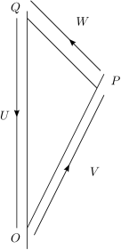
Figure 8: Illustration of the geometry and orientation of the $U$, $V$ and $W$ segments.

In this appendix, we use the perturbative solution of the geodesic and parallel transport equations, obtained in Appendix A, to find an explicit linearized expression for the time delay observable, which was defined implicitly in Sec. II. We summarize below the relevant results, whose detailed derivation can be found in Sec. V of Khavkine (2012).

First, we need to briefly recall some notation introduced in Appendix A and introduce some more. Recall that a lab-equipped spacetime $(M,g,O,\hat{e})$ defines a geodesic triangle $OPQ$ in $(M,g)$, as illustrated in Fig. 1. Minkowski space defines a special lab-equipped spacetime $(M,\eta,0,\hat{x})$, for which the geodesic triangle and its geometry, including the corresponding emission and delay times, can be computed explicitly. We parametrize the deviation of $(M,g,O,\hat{e})$ from $(H,\eta,0,\hat{x})$ with the space-time dependent general linear transformation $T=\exp(h)$ and the Lorentz transformation $L=\exp(h_{O})$ at $O$, according to Eqs. (105) and (106).

Denote the sides of the geodesic $OPQ$ triangle by the triple $(\tilde{V},\tilde{W},\tilde{U})$, oriented as shown in Fig. 8. The corresponding initial tangent vectors, which can be used to define these geodesic segments according to the scheme of Appendix A, illustrated in Fig. 7, are $(\tilde{t}\tilde{v}^{a},\tilde{w}^{a},-s\tilde{u}^{a})$, where $\tilde{w}^{a}$ is null, $\tilde{u}^{a}$ is a unit vector, $\tilde{v}^{a}=v^{i}\hat{e}^{a}_{i}$ and $\tilde{t}=\tau_{v}(s)$ is the emission time, with $s$ and $v^{i}$ fixed by the experimental protocol. In Minkowski space, these specialize to $(V,W,U)$ and $(\tau_{\mathrm{cl}}v^{a},w^{a},-su^{a})$, where

$$u^{a} =u^{i}\hat{x}^{a}_{i}=\hat{x}^{a}_{0},$$ (124)

$$w^{a} =s(u^{i}-e^{-\theta}v^{i})\hat{x}^{a}_{i},$$ (125)

$$\tau_{\mathrm{cl}}(s) =se^{-\theta}=s\sqrt{\frac{1-\frac{v_{rel}}{c}}{1+\frac{v_{rel}}{c}}},$$ (126)

with the probe rapidity $\theta$, or equivalently its relative velocity $v_{rel}$, defined by

$$u\cdot v=-\cosh\theta=-\frac{1}{\sqrt{1-(\frac{v_{rel}}{c})^{2}}}.$$ (127)

We parametrize the analogous non-Minkowski objects as

$$\tilde{t} =e^{\tilde{r}}\tau_{\mathrm{cl}}(s),$$ (128)

$$\tilde{v}^{a} =v^{i}\hat{e}^{a}_{i}=e^{a}_{i}\exp(h_{O})^{i}_{j}v^{j},$$ (129)

$$\tilde{u}^{a} =e^{a}_{i}[\exp(p_{U})\exp(p_{W})\exp(p_{V})]^{i}_{j}\exp(h_{O})^{j}_{k}u^{k},$$ (130)

$$\tilde{w}^{a} =e^{a}_{i}\exp(\tilde{q})^{i}_{j}w^{j},$$ (131)

where we have used $\exp(p_{\gamma})$ to denote the parallel transport operator along $\gamma$ as defined in Eq. (115), and we parametrized the changes in $\tilde{t}$ and $\tilde{w}$ due to the curvature by $\exp(\tilde{r})$, where $\tilde{r}$ is a scalar, and $\exp{\tilde{q}}$ is a Lorentz transformation. These are determined by the triangle closure condition (the requirement that the $\tilde{U}$ segment ends in $O$ with tangent vector $-su^{a}$). Since we are working at linear order, we only need the leading terms in the expansion of these unknowns

$$\tilde{q}^{i}_{j}=q^{i}_{j}[h]+\mathcal{O}(h^{2}),\quad\tilde{r}=r[h]+\mathcal{O}(h^{2}).$$ (132)

We have the following linearized expression for the emission time

$$\tau(s) =\tau_{\mathrm{cl}}(s)[1+r[h]+\mathcal{O}(h^{2})],$$ (133)

$$r[h] =-\frac{w^{i}J_{i}-w^{i}H_{ij}su^{j}}{\tau_{\mathrm{cl}}(s)v\cdot w},$$ (134)

where $r[h]$ was obtained from the explicitly expressed triangle closure condition, using the Eqs. (122b) and (123b) (truncated at linear order). The normalization factor explicitly evaluates to

$$\tau_{\mathrm{cl}}(s)v\cdot w=\frac{s^{2}}{2}(1-e^{-2\theta})=s^{2}\frac{\frac{v_{rel}}{c}}{(1+\frac{v_{rel}}{c})}.$$ (135)

The $H$ and $J$ terms are given explicitly by the formulas

$$w^{i}H_{ij}su^{j} =\sum_{X=V,W,U}\left(sw^{i}u^{j}\left[h_{[ij]}\right]_{x_{1}}^{x_{2}}+2sw^{[i}u^{j]}x^{k}\int_{X}\!\mathrm{d}{t}\,\partial_{i}h_{(kj)}\right),$$ (136)

$$w^{i}J_{i} =\sum_{X=V,W,U}\left(-w^{i}x^{j}\int_{X}\mathrm{d}{t}\,h_{(ij)}+2w^{[i}x^{j]}x^{k}\int_{X}^{(1)}\mathrm{d}{t}\,\partial_{i}h_{(kj)}+\sum_{X>Y=V,W,U}2w^{[i}x^{j]}y^{k}\int_{Y}\mathrm{d}{t}\,\partial_{i}h_{(kj)}\right),$$ (137)

where $\int^{(n)}_{X}$ denotes the affinely $[0,1]$-parametrized, $n$-iterated integral over the segment $X$ with tangent vector $x^{a}$ (similarly for $Y$ and $y^{a}$). An ordinary integral is $0$-iterated $\int^{(0)}\mathrm{d}{t}\,f(t)=\int_{0}^{1}\mathrm{d}{t}\,f(t)$ and $\int^{(1)}\mathrm{d}{t}f(t)=\int_{0}^{1}\mathrm{d}{t}\int_{0}^{t}\mathrm{d}{t^{\prime}}\,f(t^{\prime})$. The segments are implicitly ordered $V<W<U$. The first summand term in $H$ depends only on the antisymmetrization $h_{[ij]}$. Since we shall only use a gauge where $h_{ij}$ is symmetric, it will can always be neglected in the sequel.

The above linearized expression for $\tau(s)$ is invariant under linearized gauge transformations (in fact each of the $H$ and $J$ terms is invariant separately), which has been checked explicitly in the Appendix of Khavkine (2012).

Appendix C Calculation of the graviton two-point function

In this appendix, we calculate the Hadamard two-point function, $\langle\{\hat{h}_{ij}(x),\hat{h}_{kl}(y)\}\rangle$, for the linearly quantized graviton field $\hat{h}_{ij}(x)$, which was defined in Appendix A. Obviously, this two-point function depends on the choice of vacuum state used in the expectation value. In a linear quantum field theory, the choice of vacuum can be effectively made by identifying a suitable notion of positive frequency Hollands and Wald (2010); Birrell and Davies (1984). The standard, Poincaré invariant Fock vacuum corresponds to positive frequency with respect to any inertial time coordinate consistent with the time-orientation of our Minkowski space $(M,\eta)$. With this choice fixed, it is well known that the Hadamard two-point function is obtained from the field commutator $[\hat{h}_{ij}(x),\hat{h}_{kl}(y)]$ by flipping the sign of its negative frequency Fourier modes. Finally, the field commutator is determined by proportionality to the classical Poisson bracket, which is fully fixed by the classical Lagrangian and a choice of gauge fixing. Evidently, the result depends on the choice of gauge fixing. However, if the Hadamard two-point function is only used to evaluate expectation values of the form $\langle\{O_{1}[\hat{h}],O_{2}[\hat{h}]\}\rangle$, where $O_{1}$ and $O_{2}$ are linear gauge invariant observables, these expectation values will not depend on the choice of gauge, nor even on the addition to the Hadamard two-point function of anything that is annihilated in the process. This last observation allows us to choose, in the end, a particularly simple and symmetric expression for the Hadamard two-point function. All these steps are performed below.

C.1 Field commutator

The field commutator is fixed, according to the usual rules of canonical quantization, by the formula

$$[\hat{h}_{ij}(x),\hat{h}_{kl}(y)]=i\hbar\,\Pi(h_{ij}(x),h_{kl}(y)),$$ (138)

where we use $\Pi(-,-)$ to denote the classical Poisson bracket to distinguish it from the quantum anti-commutator $\{-,-\}$. In a gauge theory, Poisson brackets are usually defined only on gauge invariant observables, but are essentially fixed by the Lagrangian density. To extend Poisson brackets to noninvariant observables, like the field evaluations $h_{ij}(x)$, we must also specify a gauge fixing. Below, we use the transverse-traceless-radiation condition (Wald, 1984, Sec.4.4b), which fully fixes the available gauge freedom.

To determine the Poisson brackets, instead of going through a complicated 3+1 decomposition and the associated constraint analysis, we follow the covariant phase space formalism Lee and Wald (1990). The Lagrangian, together with a choice of Cauchy surface, naturally determines a 2-form on the space of (off-shell) field configurations. This 2-form, when restricted to the subspace of solutions (on-shell), becomes presymplectic and independent of the choice of the Cauchy surface. Further, restricting to the subspace gauge fixed solution, which we identify with the physical phase space, it becomes symplectic. We explicitly invert this symplectic form to obtain the Poisson bivector and hence the Poisson brackets.

C.1.1 Lagrangian

Since we are interested in linearized gravity, we start with Minkowski space $(M,\eta)$ and a global inertial coordinate system $x^{\mu}$ thereon. For our action, we take the Einstein-Palatini action Deser (1970), which in coordinates looks like

$$S_{EP} =\int\mathrm{d}^{4}{x}\,\mathcal{L}_{EP}=\kappa\int\mathrm{d}^{4}{x}\,\tilde{g}^{\mu\nu}R_{\mu\nu},$$ (139)

$$R_{\mu\nu} =\left(\partial_{\lambda}\Gamma^{\lambda}_{\mu\nu}-\partial_{\nu}\Gamma^{\lambda}_{\mu\lambda}+\Gamma^{\lambda}_{\nu\mu}\Gamma^{\beta}_{\lambda\beta}-\Gamma^{\lambda}_{\beta\mu}\Gamma^{\beta}_{\lambda\nu}\right),$$ (140)

where $R_{\mu\nu}$ the Ricci tensor, built entirely out of the Christoffel symbols $\Gamma^{\lambda}_{\mu\nu}$, and $\tilde{g}^{\mu\nu}$ is the inverse densitized metric, i.e., $g_{\mu\nu}\tilde{g}^{\nu\lambda}=\sqrt{-g}\delta_{\mu}^{\lambda}$, with $g$ the determinant of $g_{\mu\nu}$.

The independent fields in the Einstein-Palatini action are $\tilde{g}^{\mu\nu}$ and $\Gamma^{\lambda}_{\mu\nu}$. The Christoffel symbols are auxiliary (they can be eliminated algebraically through their own equations of motion) and their elimination immediately establishes equivalence with the vacuum Einstein equations. It remains only to fix the overall constant $\kappa$.

To find this constant, we consider the joint gravity-matter action $S_{EP}+S_{M}$, where $S_{M}$ is the action of a point particle, and impose on it two conditions: in the nonrelativistic limit (i) $S_{M}$ has the standard kinetic term $\int\mathrm{d}{t}\,\frac{mv^{2}}{2}$ and (ii) the equations of motion reproduce the standard Poisson equation for the Newtonian gravitational potential of a particle of mass $m$. It is well known (Landau and Lifshitz, 1980, Eq. 8.1) that (i) is satisfied by

$$S_{M}=-mc\int\!\mathrm{d}{\tau}\,\sqrt{-\dot{\gamma}^{\mu}(\tau)\dot{\gamma}^{\nu}(\tau)g_{\mu\nu}},$$ (141)

where $\gamma^{\mu}(\tau)$ are the coordinates of the particle’s worldline. Variation of the total action yields the Einstein equations in a form equivalent to

$$R_{\mu\nu}-\frac{1}{2}g_{\mu\nu}R=\frac{c^{3}}{2\kappa}T_{\mu\nu},$$ (142)

where $R=g^{\mu\nu}R_{\mu\nu}$ is the Ricci scalar and the stress-energy tensor of the point particle has the expected form

$$T_{\mu\nu}(x)=\int\mathrm{d}\sigma\,mc^{2}u_{\mu}u_{\nu}\,\delta(x,\gamma(\sigma)),$$ (143)

with $\mathrm{d}\sigma=\sqrt{-\dot{\gamma}^{\nu}\dot{\gamma}^{\lambda}g_{\nu\lambda}}\mathrm{d}\tau$, $u^{\mu}=\dot{\gamma}^{\mu}/\sqrt{-\dot{\gamma}^{\nu}\dot{\gamma}^{\lambda}g_{\nu\lambda}}$ and $\delta(x,y)\sqrt{-g}=\delta^{4}(x-y)$, respectively, the proper time line element, the unit $4$-velocity and the scalar Dirac distribution. The correct Newtonian limit is recovered, equivalently, (ii) is satisfied, if $c^{3}/2\kappa=8\pi G$ (Landau and Lifshitz, 1980, §99) or

$$\kappa=\frac{1}{16\pi}\frac{c^{3}}{G}=\frac{1}{16\pi}\frac{\hbar}{\ell_{p}^{2}},$$ (144)

where $G$ is Newton’s gravitational constant and $\ell_{p}$ is the Planck length.

C.1.2 Gauge fixed symplectic form

Following Lee and Wald (1990), we define a 2-form $\Omega$ on the space of (off-shell) field configurations

$$\Omega=\int_{\Sigma}\omega,$$ (145)

where $\Sigma$ is a (codimension-1) Cauchy surface and $\omega$ is itself a 2-form on the space of field configurations, valued in spacetime 3-forms. We call $\omega$ the presymplectic current density. When restricted to the subspace of solutions (on-shell), it is space-time closed, $\mathrm{d}\omega=0$, as well as variationally closed, $\delta\omega=0$, where we have used $\delta$ as the exterior field variational derivative. Hence $\Omega$ is independent of $\Sigma$ and is presymplectic on the space of solutions. When dealing with a gauge theory, as we are now, its restriction $\bar{\Omega}$ to the subspace of gauge fixed solutions becomes symplectic. We calculate $\omega$ from the Lagrangian density $\mathcal{L}$ using the following steps

$$\delta\mathcal{L} =EL-\mathrm{d}\theta,$$ (146)

$$\omega =\delta\theta,$$ (147)

where we have again used $\delta$ as the exterior field variational derivative, $EL$ denotes the term proportional to the Euler-Lagrange equations and $\mathrm{d}\theta$ is the spacetime exact “boundary term” that is usually discarded while varying the action. We call $\theta$ the presymplectic potential current density.

Starting with the Einstein-Palatini action (139), we find

$$\theta =\kappa\,(\tilde{g}^{\mu\nu}\delta\Gamma^{\alpha}_{\mu\nu}-\tilde{g}^{\mu\alpha}\Gamma^{\nu}_{\mu\nu})\,\mathrm{d}^{3}{x_{\alpha}}$$ (148)

$$\omega =\kappa\,(\delta\tilde{g}^{\mu\nu}\wedge\delta\Gamma^{\alpha}_{\mu\nu}-\delta\tilde{g}^{\mu\alpha}\wedge\delta\Gamma^{\nu}_{\mu\nu})\,\mathrm{d}^{3}{x_{\alpha}},$$ (149)

where $\wedge$ denotes the anti-symmetric product of field variational forms and in our global inertial coordinates $\mathrm{d}{x^{\beta}}\wedge\mathrm{d}^{3}{x_{\alpha}}=\delta_{\alpha}^{\beta}\mathrm{d}^{4}{x}$. Letting $\Sigma$ be the hypersurface $t=x^{0}=0$, we have

$$\Omega=\kappa\int_{t=0}(\delta\tilde{g}^{\mu\nu}\wedge\delta\Gamma^{0}_{\mu\nu}-\delta\tilde{g}^{\mu 0}\wedge\delta\Gamma^{\nu}_{\mu\nu})\,\mathrm{d}^{3}{x_{0}}.$$ (150)

At this point, in one step, we restrict to gauge fixed solutions and expand everything to first perturbative order in the graviton field $h_{(ij)}$, which was defined in Appendix A, with the notation $h_{\mu\nu}=h_{(ij)}(\mathrm{d}{x^{i}})_{\mu}(\mathrm{d}{x^{j}})_{\nu}$:

$$g_{\mu\nu} =\eta_{\mu\nu}+2h_{\mu\nu}+\mathcal{O}(h^{2}),$$ (151)

$$\tilde{g}^{\mu\nu} =\eta^{\mu\nu}-2h^{\mu\nu}+\eta^{\mu\nu}h^{\alpha}_{\alpha}+\mathcal{O}(h^{2}),$$ (152)

$$\Gamma^{\alpha}_{\mu\nu} =\eta^{\alpha\beta}(\partial_{\mu}h_{\beta\nu}+\partial_{\nu}h_{\beta\mu}-\partial_{\beta}h_{\mu\nu})+\mathcal{O}(h^{2}),$$ (153)

where indices have been raised using $\eta^{\mu\nu}$. On top of the equations of motion, to fix the full available gauge freedom, we impose the transverse-traceless-radiation condition (Wald, 1984, Sec.4.4b):

$$\Box\,h_{\mu\nu} =\partial^{\lambda}\partial_{\lambda}h_{\mu\nu}=0,$$ (154)

$$\partial^{\mu}h_{\mu\nu} =0,$$ (155)

$$h^{\mu}_{\mu} =0,$$ (156)

$$t_{\mu}h^{\mu\nu} =h^{0\nu}=0,$$ (157)

where $t_{\mu}=(\mathrm{d}{t})_{\mu}$.

Making use of the above expansions and gauge fixing conditions, the form (150) restricts to the symplectic form

$$\bar{\Omega}=2\int_{t=0}\,(\delta h^{\mu\nu}\wedge\delta\dot{h}_{\mu\nu})\,\mathrm{d}^{3}{x_{0}},$$ (158)

where the dot denotes the $\partial_{0}$ derivative.

The general gauge fixed solution can be explicitly written in Fourier space, with $x=(t,\mathbf{x})$, $k=(\omega,\mathbf{k})$ and $\omega_{k}=|\mathbf{k}|$, as

$$h_{\mu\nu}(x)=\int\frac{\mathrm{d}^{3}{\mathbf{k}}}{(2\pi)^{3}}\,e^{i\mathbf{k}\cdot\mathbf{x}}\\ {}\times(P^{1}_{\mu\nu}(k)[\alpha^{+}_{1}(k)e^{-i\omega_{k}t}+\alpha^{-}_{1}(k)e^{i\omega_{k}t}]\\ {}+P^{2}_{\mu\nu}(k)[\alpha^{+}_{2}(k)e^{-i\omega_{k}t}+\alpha^{-}_{2}(k)e^{i\omega_{k}t}]),$$ (162)

where $\alpha_{i}^{\pm}(k)$ are arbitrary $k$-dependent coefficients and $P^{i}_{\mu\nu}$ are polarization factors that need to satisfy

$$\eta^{\mu\nu}P^{i}_{\mu\nu} =0,$$ (163)

$$t^{\mu}P^{i}_{\mu\nu} =P^{i}_{0\nu}=0,$$

$$k^{\mu}P^{i}_{\mu\nu} =0,$$

$$P^{i}_{\mu\nu}P^{j\,\mu\nu} =\delta^{ij},$$

$$P^{1}_{\mu\nu}(-k)=P^{1}_{\mu\nu}(k), \quad P^{2}_{\mu\nu}(-k)=-P^{2}_{\mu\nu}(k),$$

for $i=1,2$. The first three conditions are directly related to the gauge fixing, the orthogonality condition ensures that the coefficients $\alpha^{\pm}_{i}$ describe independent polarizations for different $i$, and the last conditions prescribe their behavior under parity transformations . In the final expression for the Poisson bracket, only the projected identity tensor $P^{1}_{\mu\nu}P^{1}_{\lambda\kappa}+P^{2}_{\mu\nu}P^{2}_{\lambda\kappa}$ appears explicitly. So, instead of finding explicit expressions for the polarization factors and computing the projected identity from its definition, we simplify the calculation by expressing it in the most general basis and then restricting the coefficients using all of the above conditions. As a basis, we use all rank-4 tensors that could be constructed from $\eta_{\mu\nu}$, $t_{\mu}$, and $k_{\mu}$ that are symmetric under the index exchanges $(\mu\nu)\leftrightarrow(\kappa\lambda)$, $\mu\leftrightarrow\nu$ and $\kappa\leftrightarrow\lambda$:

$$P^{1}_{\mu\nu}P^{1}_{\kappa\lambda}+P^{2}_{\mu\nu}P^{2}_{\kappa\lambda} =\frac{1}{2}\left(\eta_{\mu\kappa}\eta_{\nu\lambda}+\eta_{\mu\lambda}\eta_{\nu\kappa}\right)+A\,\eta_{\mu\nu}\eta_{\kappa\lambda}+B\left(\eta_{\mu\nu}k_{\kappa}k_{\lambda}+\eta_{\kappa\lambda}k_{\mu}k_{\nu}\right)$$ (164)

$$\quad{}+C\left(\eta_{\mu\kappa}k_{\nu}k_{\lambda}+\eta_{\nu\kappa}k_{\mu}k_{\lambda}+\eta_{\mu\lambda}k_{\nu}k_{\kappa}+\eta_{\nu\lambda}k_{\mu}k_{\kappa}\right)+D\left(\eta_{\mu\nu}t_{\kappa}t_{\lambda}+\eta_{\kappa\lambda}t_{\mu}t_{\nu}\right)$$

$$\quad{}+E\left(\eta_{\mu\kappa}t_{\nu}t_{\lambda}+\eta_{\nu\kappa}t_{\mu}t_{\lambda}+\eta_{\mu\lambda}t_{\nu}t_{\kappa}+\eta_{\nu\lambda}t_{\mu}t_{\kappa}\right)+F\left(\eta_{\mu\nu}k_{\kappa}t_{\lambda}+\eta_{\mu\nu}k_{\lambda}t_{\kappa}+\eta_{\kappa\lambda}k_{\mu}t_{\nu}+\eta_{\kappa\lambda}k_{\nu}t_{\mu}\right)$$

$$\quad{}+G\left(\eta_{\mu\kappa}k_{\nu}t_{\lambda}+\eta_{\nu\kappa}k_{\mu}t_{\lambda}+\eta_{\mu\lambda}k_{\nu}t_{\kappa}+\eta_{\nu\lambda}k_{\mu}t_{\kappa}\right)+H\left(\eta_{\mu\kappa}k_{\lambda}t_{\nu}+\eta_{\nu\kappa}k_{\lambda}t_{\mu}+\eta_{\mu\lambda}t_{\nu}k_{\kappa}+\eta_{\nu\lambda}t_{\mu}k_{\kappa}\right)$$

$$\quad{}+I\,k_{\mu}k_{\nu}k_{\kappa}k_{\lambda}+J\left(k_{\mu}k_{\nu}k_{\kappa}t_{\lambda}+k_{\mu}k_{\nu}k_{\lambda}t_{\kappa}+k_{\mu}k_{\kappa}k_{\lambda}t_{\nu}+k_{\nu}k_{\kappa}k_{\lambda}t_{\mu}\right)$$

$$\quad{}+K\left(k_{\mu}k_{\nu}t_{\kappa}t_{\lambda}+k_{\kappa}k_{\lambda}t_{\mu}t_{\nu}\right)+L\left(k_{\mu}k_{\kappa}t_{\nu}t_{\lambda}+k_{\mu}k_{\lambda}t_{\nu}t_{\kappa}+k_{\nu}k_{\kappa}t_{\mu}t_{\lambda}+k_{\nu}k_{\lambda}t_{\mu}t_{\kappa}\right)$$

$$\quad{}+M\left(k_{\mu}t_{\nu}t_{\kappa}t_{\lambda}+k_{\nu}t_{\mu}t\kappa t_{\lambda}+k_{\kappa}t_{\mu}t_{\nu}t_{\lambda}+k_{\lambda}t_{\mu}t_{\nu}t_{\kappa}\right)+N\,t_{\mu}t_{\nu}t_{\kappa}t_{\lambda}$$

where the capital letters are constants that will be fixed by the restrictions in (163). We have 14 constants: the trace condition gives four independent constraints and projection onto $t^{\mu}$ and $k^{\mu}$ each give ten constraints amounting to a total of 24 constraints. Fortunately, some constraints are redundant and the system is exactly solvable. Having set $t^{2}=-1$, we obtain the following expressions for the constants:

$$A =-\frac{1}{2}, H =\frac{-k\cdot t}{2\left(k^{2}+(k\cdot t)^{2}\right)},$$

$$B =\frac{1}{2\left(k^{2}+(k\cdot t)^{2}\right)}, I =\frac{1}{2\left(k^{2}+(k\cdot t)^{2}\right)^{2}},$$

$$C =-\frac{1}{2\left(k^{2}+(k\cdot t)^{2}\right)}, J =\frac{k\cdot t}{2\left(k^{2}+(k\cdot t)^{2}\right)^{2}},$$

$$D =-\frac{k^{2}}{2\left(k^{2}+(k\cdot t)^{2}\right)}, K =\frac{k^{2}+2(k\cdot t)^{2}}{2\left(k^{2}+(k\cdot t)^{2}\right)^{2}},$$

$$E =\frac{k^{2}}{2\left(k^{2}+(k\cdot t)^{2}\right)}, L =-\frac{k^{2}}{2\left(k^{2}+(k\cdot t)^{2}\right)^{2}},$$

$$F =\frac{k\cdot t}{2\left(k^{2}+(k\cdot t)^{2}\right)}, M =-\frac{k^{2}(k\cdot t)}{2\left(k^{2}+(k\cdot t)^{2}\right)^{2}},$$

$$G =-\frac{k\cdot t}{2\left(k^{2}+(k\cdot t)^{2}\right)}, N =\frac{k^{4}}{2\left(k^{2}+(k\cdot t)^{2}\right)^{2}}.$$

The resulting projected identity is rather long and complicated. Conveniently, there are some simplifications that can be made. Since $h_{\mu\nu}$ has gauge degrees of freedom of the form $k_{(\mu}\zeta_{\nu)}$, all terms that have a similar form can consequently be gauged away when calculating observables. Additionally, the projected identity will appear in the graviton two-point function within an integral over $k$ together with $\delta^{(4)}(k^{2})$; hence all terms that are proportional to $k^{2}$ will vanish. Ergo, the only nonvanishing constant is $A=-\frac{1}{2}$ and, for the purpose of calculating with gauge invariant observables, the projected identity can be taken to be simply

$$P^{1}_{\mu\nu}P^{1}_{\kappa\lambda}+P^{2}_{\mu\nu}P^{2}_{\kappa\lambda} =\frac{1}{2}\left(\eta_{\mu\kappa}\eta_{\nu\lambda}+\eta_{\mu\lambda}\eta_{\nu\kappa}-\eta_{\mu\nu}\eta_{\kappa\lambda}\right)$$

$$\equiv\frac{1}{2}\eta_{\mu\nu,\kappa\lambda}.$$ (165)

Inserting the general gauge fixed solution (162) into the symplectic form, expression (158), gives

$$\bar{\Omega} =2\kappa\int_{t=0}\mathrm{d}^{3}{\mathbf{x}}\int\frac{\mathrm{d}^{3}{\mathbf{k}}}{(2\pi)^{3}}\int\frac{\mathrm{d}^{3}{\mathbf{k}^{\prime}}}{(2\pi)^{3}}\,i\omega_{k^{\prime}}e^{i(\mathbf{k}+\mathbf{k}^{\prime})\cdot\mathbf{x}}$$

$${}\times\left(P^{1\,\mu\nu}(k)[\delta\alpha^{+}_{1}(k)e^{-i\omega_{k}t}+\delta\alpha^{-}_{1}(k)e^{i\omega_{k}t}]\right.$$

$$\quad\left.{}+P^{2\,\mu\nu}(k)[\delta\alpha^{+}_{2}(k)e^{-i\omega_{k}t}+\delta\alpha^{-}_{2}(k)e^{i\omega_{k}t}]\right)$$ (166)

$$\wedge\left(P^{1}_{\mu\nu}(k^{\prime})[-\delta\alpha^{+}_{1}(k^{\prime})e^{-i\omega_{k^{\prime}}t}+\delta\alpha^{-}_{1}(k^{\prime})e^{i\omega_{k^{\prime}}t}]\right.$$

$$\quad\left.{}+P^{2}_{\mu\nu}(k^{\prime})[-\delta\alpha^{+}_{2}(k^{\prime})e^{-i\omega_{k^{\prime}}t}+\delta\alpha^{-}_{2}(k^{\prime})e^{i\omega_{k^{\prime}}t}]\right)$$

$$=4\kappa\int_{\mathbb{R}^{3}_{+}}\frac{\mathrm{d}^{3}{\mathbf{k}}}{(2\pi)^{3}}\,i\omega_{k}$$

$$\qquad{}\times\left(-\delta\alpha_{1}^{+}\wedge\delta\alpha_{1}^{+*}+\delta\alpha_{1}^{-}\wedge\delta\alpha_{1}^{-*}\right.$$ (167)

$$\qquad\quad\left.{}-\delta\alpha_{2}^{+}\wedge\delta\alpha_{2}^{+*}+\delta\alpha_{2}^{-}\wedge\delta\alpha_{2}^{-*}\right).$$

This result requires some explanation. The $\mathbf{x}$-integration results in a factor of $\delta^{3}(\mathbf{k}+\mathbf{k}^{\prime})$, which eliminates the $\mathbf{k}^{\prime}$-integral. Further, the reality of the graviton field, $h^{*}_{\mu\nu}(x)=h_{\mu\nu}(x)$, and the parity properties of $P^{i}_{\mu\nu}(k)$ given in (163) translate to the following parity properties of the $\alpha^{\pm}_{i}$ coefficients:

$$\alpha_{1}^{+}(k) =\alpha_{1}^{-*}(-k),$$ (168)

$$\alpha_{1}^{-}(k) =\alpha_{1}^{+*}(-k),$$

$$\alpha_{2}^{+}(k) =-\alpha_{2}^{-*}(-k),$$

$$\alpha_{2}^{-}(k) =-\alpha_{2}^{+*}(-k).$$

Taking these parity properties into account, the integration domain can then be shrunk from all of $\mathbb{R}^{3}$ to $\mathbb{R}^{3}_{+}$, the half-space satisfying $k_{z}\geq 0$. Effecting the remaining algebraic simplifications gives the expression (167), where the argument of each $\alpha$-coefficient is $+k$ and hence has been omitted for conciseness. Each of the $\alpha$-coefficients appearing in (167) is now independent of the others, at fixed $\mathbf{k}$ and at other values of $\mathbf{k}\in\mathbb{R}^{3}_{+}$.

C.1.3 Gauge fixed Poisson brackets

If we consider the $\alpha^{\pm}_{i}(k)$-coefficients as a complete set of independent coordinates on the physical phase space of linearized gravity, then the expression (167) for the symplectic form shows that they are also canonical. Therefore, it is straightforward to write down the Poisson bivector $\Pi=\bar{\Omega}^{-1}$:

$$\Pi =\frac{1}{4\kappa}\int_{\mathbb{R}^{3}_{+}}\mathrm{d}^{3}{k}\,\frac{(2\pi)^{3}}{ik}$$

$$\qquad{}\times\left(-\partial_{\alpha_{1}^{+}}\wedge\partial_{\alpha_{1}^{+*}}+\partial_{\alpha_{1}^{-}}\wedge\partial_{\alpha_{1}^{-*}}\right.$$ (169)

$$\qquad\quad\left.{}-\partial_{\alpha_{2}^{+}}\wedge\partial_{\alpha_{2}^{+*}}+\partial_{\alpha_{2}^{-}}\wedge\partial_{\alpha_{2}^{-*}}\right),$$

where the field variational vector fields $\partial_{\alpha^{\pm}_{i}}$ for are dual to the field variational $1$-forms $\delta\alpha^{\pm}_{i}$. These vector fields, through the standard action of vectors and bivectors on functions, also satisfy the following identities, which follow from the parity properties (168):

$$\partial_{\alpha_{1}^{+}(k)}\alpha^{+}_{1}(q) =\delta(\mathbf{k}-\mathbf{q}),$$

$$\partial_{\alpha_{1}^{+}(k)}\wedge\partial_{\alpha_{1}^{+}(k)^{*}}\left(\alpha^{+}_{1}(p),\alpha^{-}_{1}(q)\right) =\delta(\mathbf{k}-\mathbf{p})\delta(\mathbf{k}+\mathbf{q}),$$

$$\partial_{\alpha_{1}^{+}(k)}\wedge\partial_{\alpha_{1}^{+}(k)^{*}}\left(\alpha^{+}_{1}(p),\alpha^{+}_{1}(q)\right) =0,$$

$$\partial_{\alpha_{1}^{-}(k)}\wedge\partial_{\alpha_{1}^{-}(k)^{*}}\left(\alpha^{+}_{1}(p),\alpha^{-}_{1}(q)\right) =-\delta(\mathbf{k}-\mathbf{p})\delta(\mathbf{k}+\mathbf{q}),$$

$$\partial_{\alpha_{2}^{+}(k)}\wedge\partial_{\alpha_{2}^{+}(k)^{*}}\left(\alpha^{+}_{2}(p),\alpha^{-}_{2}(q)\right) =-\delta(\mathbf{k}-\mathbf{p})\delta(\mathbf{k}+\mathbf{q}),$$

$$\partial_{\alpha_{2}^{-}(k)}\wedge\partial_{\alpha_{2}^{-}(k)^{*}}\left(\alpha^{+}_{2}(p),\alpha^{-}_{2}(q)\right) =\delta(\mathbf{k}-\mathbf{p})\delta(\mathbf{k}+\mathbf{q}).$$

Finally, using the above identities, together with the explicit parametrization (162) of gauge fixed solutions, the explicit formula (169) for the Poisson bivector and the simplified expression (165) for the projected identity tensor, we obtain the Poisson brackets of two graviton field evaluations

$$\Pi(h_{\mu\nu}(x),h_{\kappa\lambda}(y))$$

$$=\frac{2\pi}{4\kappa i}\int\!\!\frac{\mathrm{d}^{4}{k}}{(2\pi)^{4}}\,\delta(k^{2})\left(P^{1}_{\mu\nu}P^{1}_{\kappa\lambda}+P^{2}_{\mu\nu}P^{2}_{\kappa\lambda}\right)e^{ik\cdot(x-y)}\text{sgn}(\omega)$$

$$=\frac{1}{2}\,\frac{2\pi}{4\kappa i}\,\eta_{\mu\nu,\kappa\lambda}\int\frac{\mathrm{d}^{4}{k}}{(2\pi)^{4}}\,\delta(k^{2})e^{ik\cdot(x-y)}\text{sgn}(\omega),$$ (170)

where $\text{sgn}(x)$ is the sign-function and as before $k=(\omega,\mathbf{k})$, with the extra integration over $\omega$ compensated by the $\delta(k^{2})$ factor and the various $e^{\pm i\omega_{k}t}$ factors absorbed into the single remaining exponential.

C.2 Sign flip

Having computed the Poisson brackets of field evaluations in the gauge fixed, linear, classical graviton field theory, canonical quantization uniquely fixes the commutator of the corresponding quantum field operators:

$$[\hat{h}_{\mu\nu}(x),\hat{h}_{\kappa\lambda}(y)]=i\hbar\Pi(h_{\mu\nu}(x),h_{\kappa\lambda}(y)).$$ (171)

As mentioned earlier, it is well known Hollands and Wald (2010); Birrell and Davies (1984) that the above field commutator is related to the Hadamard two-point function by a flip of the sign of its negative frequency components:

$$\langle\{\hat{h}_{\mu\nu}(x),\hat{h}_{\kappa\lambda}(y)\}\rangle$$

$$=i\hbar\,\text{sgn}(i\partial_{t})\,\Pi(h_{\mu\nu}(x),h_{\kappa\lambda}(y))$$ (172)

$$=\frac{\hbar}{2}\,\frac{2\pi}{4\kappa}\,\eta_{\mu\nu,\kappa\lambda}\int\frac{\mathrm{d}^{4}{k}}{(2\pi)^{4}}\,\delta(k^{2})e^{ik\cdot(x-y)}$$ (173)

$$=\eta_{\mu\nu,\kappa\lambda}\,\frac{\ell_{p}^{2}}{\pi}P\left[\frac{1}{(x-y)^{2}}\right],$$ (174)

where the symbol $P$ denotes the Cauchy principal value prescription and we have used the identity Gelʹfand and Shilov (1964)

$$\int\frac{\mathrm{d}^{4}k}{(2\pi)^{4}}\,\delta(k^{2})e^{ik\cdot x}=\frac{2}{(2\pi)^{3}}P\frac{1}{x^{2}}$$ (175)

and the value $\kappa=\frac{1}{16\pi}\frac{\hbar}{\ell_{p}^{2}}$ from Eq. (144). We should note that Eq. (175) is an identity involving two distributions, a Dirac-delta and a Cauchy principal value, which are strictly defined only when their arguments have simple zeros and poles, respectively. Unfortunately, this condition fails precisely at $k=0$ and $x=0$, respectively, so the distributions are only defined in the complements of these points. However, in four dimensions, each distribution can be uniquely extended to the excluded point provided that it remains homogeneous Gelʹfand and Shilov (1964).

Appendix D Calculation of partial check

As a partial check on our computer routine, we calculated—for a very specific case—the smeared integral $\tilde{I}^{00}$ ($|K|=0$) by hand. In particular, we considered the integral along two coinciding (hence parallel) 0-iterated null line segments. This case was chosen because of its fairly simple calculation and limited number of intermediate steps. Indeed all results in this appendix are reproduced by our computer routine.

We calculated the following integral along two parallel null line segments

$$\tilde{I}^{00}=\int\!\mathrm{d}^{4}{z}\int_{0}^{1}\!\mathrm{d}{s}\int_{0}^{1}\!\mathrm{d}{t}\,P\frac{g(z_{\perp}^{2})\delta(u\cdot z)}{\left(x(s)-y(t)-z\right)^{2}}.$$ (176)

We consider the null segments $x=y=\lambda(u-{\hat{u}})$, for some scalar $\lambda$, so that $x(s)=sx$ with $\lambda$ and $y(t)=ty=tx$. Since $x^{2}=y^{2}=0$ and $z\cdot x=-\lambda(c-T)$, we can rewrite the denominator as

$$((s-t)x-z)^{2} =z^{2}+2(t-s)x\cdot z$$ (177)

$$=R^{2}-T^{2}-2\lambda(t-s)(c-T).$$ (178)

Parametrizing the integral in a similar manner as in Sec. IV and rearranging the denominator gives

$$\tilde{I}^{00}=-\int_{0}^{2\pi}\!\mathrm{d}{\phi}\underbrace{\int_{-\infty}^{\infty}\!\mathrm{d}{T}\delta^{(d)}(-T)\int_{0}^{\infty}\!\mathrm{d}{R}\,R\,g(R^{2})\,}_{\text{part II}}\\ {}\times\underbrace{\int^{1}_{0}\!\mathrm{d}{s}\int^{1}_{0}\!\mathrm{d}{t}\int_{-R}^{R}\!\mathrm{d}{c}P\,\frac{1}{R^{2}-T^{2}-2\lambda(t-s)(c-T)}}_{\text{part I}}.$$ (181)

To compute this integral, we follow the same logic that the computer algebra uses: “part I” first, which amounts to performing the integration over $c$, $s$ and $t$, and subsequently, “part II”, which entails integration over $R$ and $T$. The $\phi$ integral merely contributes an overall factor of $2\pi$. Integration over $c$ yields

$$\int_{-R}^{R}\!\mathrm{d}{c}\,\frac{1}{R^{2}-T^{2}-2\lambda(t-s)(c-T)}\\ =\left[-\frac{\left(\ln|c-T|+\ln|c+T-2\lambda(t-s)|\right)}{2\lambda(t-s)}\right]_{-R}^{R}.$$ (184)

For simplicity, below, we work with the expression inside the square brackets and plug in the boundary values $c=\pm R$ at the end. Next, integration along $s$ and $t$ is performed. The first term in (184) gives

$$\int\!\mathrm{d}{s}\int\!\mathrm{d}{t}\left(-\frac{\ln|c-T|}{2\lambda(t-s)}\right)\\ =-\frac{1}{2\lambda}\ln|c-T|\left[\left[-(t-s)\left(\ln|t-s|-1\right)\right]\right],$$

where the square brackets indicate that the boundaries of $s$ and $t$ still need to be inserted. These boundaries correspond to the four vertices in Fig. 3. The second term in (184) yields

$$\int\!\mathrm{d}{s}\!\int\!\mathrm{d}{t}\left(-\frac{\ln|c+T-2\lambda(t-s)|}{2\lambda(t-s)}\right)\\ =-\frac{\ln|c+T|}{2\lambda}\left[\left[-(t-s)\left(\ln|t-s|-1\right)\right]\right]+\frac{1}{2\lambda}[[(t-s)]]\\ -\frac{1}{2\lambda}\left[\left[\left(t-s-\frac{c+T}{2\lambda}\right)\ln\Big{|}1-\frac{2\lambda(t-s)}{c+T}\Big{|}\right.\right.\\ \left.\left.+(t-s)L\left(\frac{2\lambda(t-s)}{c+T}\right)\right]\right].$$

After combining the two equations again and extracting the logarithmic divergences from the dilogarithm by applying Eq. (82), we obtain an expression of the form $-\frac{1}{2\lambda}[[\cdots]]$, where the double square brackets enclose

$$-\ln\left|c^{2}-T^{2}\right|(t-s)\left(\ln|t-s|-1\right)-(t-s)\\ +\left((t-s)-\frac{c+T}{2\lambda}\right)\ln\left|1-\frac{2\lambda(t-s)}{c+T}\right|\\ -(t-s)\operatorname{L}\left(\frac{c+T}{2\lambda(t-s)}\right)-\frac{(t-s)}{2}\left(\ln\left|\frac{c+T}{2\lambda(t-s)}\right|\right)^{2}\\ +\frac{\pi^{2}}{12}(t-s)+\frac{\pi^{2}}{4}(t-s)\text{sgn}\left(\frac{c+T}{2\lambda(t-s)}\right).$$

Evaluating this result at the boundaries $(s,t)=(0,0)$ and $(s,t)=(1,1)$ which correspond to the $z_{11}$ and $z_{22}$ vertices gives zero. The $(s,t)=(1,0)$ and $(s,t)=(0,1)$ boundaries which map to the $z_{12}$ and $z_{21}$ vertices give a nonzero result given by

$$-\frac{1}{2\lambda}\Biggl{(}\frac{\ln|1+\frac{2\lambda}{c+T}|}{\ln|1-\frac{2\lambda}{c+T}|}+\frac{(c+T)}{2\lambda}\ln\biggl{|}1-\left(\frac{2\lambda}{c+T}\right)^{2}\biggr{|}\\ +\operatorname{L}\left(\frac{c+T}{2\lambda}\right)-\operatorname{L}\left(-\frac{c+T}{2\lambda}\right)-\frac{\pi^{2}}{2}\text{sgn}\left(\frac{c+T}{2\lambda}\right)\Biggr{)}.$$

Expanding this for small $c+T$ yields

$$-\frac{1}{2\lambda}\left(2\frac{c+T}{\lambda}-\frac{c+T}{\lambda}\ln\left|\frac{c+T}{2\lambda}\right|-\frac{\pi^{2}}{2}\text{sgn}\left(\frac{c+T}{2\lambda}\right)\right)\\ +\mathcal{O}(c+T)^{2},$$

where we recall that the summation over $c=\pm R$ still needs to be performed. Integration over $\phi$ and $T$ is trivial and using the definition in Eq. (85), the result is

$$\tilde{I}^{00}=\frac{\pi}{\lambda^{2}}\left(4+2\ln|2\lambda/\mu|-\frac{\pi^{2}\,\lambda}{\mu}\right)+\mathcal{O}(\mu^{0}).$$

The same calculation was also checked by hand using the momentum space representation of the Hadamard two-point function Eq. (173), with the smearing and $s,t$ integrals also converted to momentum space. The result agreed with the above, giving us confidence that it is correct. This result is also reproduced by the computer calculation, giving us confidence that the latter is correct as well.

The same procedure can also be used to calculate terms with one or two derivatives on the smearing function. However, these calculations are slightly more involved since now also terms proportional to $c$ and $c^{2}$ appear and integration by parts is needed. The results of the calculation for these integrals have been checked by hand and are quoted here without any intermediate steps. These results also agree with the computer output. For one derivative on the smearing function ($|K|=1$) we have $\tilde{I}^{00}_{u}=\tilde{I}^{00}_{{\hat{u}}}=0$. For two derivatives on the smearing function ($|K|=2$), the complete set of smeared segment integrals is

$$\tilde{I}^{00}_{uu}= \frac{\pi}{\lambda^{2}}\left(-\frac{2}{\mu^{2}}+\pi^{2}\,\lambda\,g(0)\right)+\mathcal{O}(\mu^{0}),$$

$$\tilde{I}^{00}_{u{\hat{u}}}= \frac{\pi}{\lambda^{2}}\left(-\frac{8}{\mu^{2}}-\frac{16\ln|2\lambda/\mu|}{\mu^{2}}+4\pi^{2}\,\lambda\,g(0)\right)+\mathcal{O}(\mu^{0}),$$

$$\tilde{I}^{00}_{{\hat{u}}{\hat{u}}}= \frac{\pi}{\lambda^{2}}\left(\frac{10}{\mu^{2}}-\frac{12\ln|2\lambda/\mu|}{\mu^{2}}+\pi^{2}\,\lambda\,g(0)\right)+\mathcal{O}(\mu^{0}),$$

$$\tilde{I}^{00}_{\delta_{\perp}}= \frac{\pi}{\lambda^{2}}\left(-\frac{4}{\mu^{2}}-\frac{4\ln|2\lambda/\mu|}{\mu^{2}}\right)+\mathcal{O}(\mu^{0}).$$

References

- Khavkine (2012) I. Khavkine, Physical Review D 85, 124014 (2012), arXiv:1111.7127v2 .
- Bergmann (1961) P. G. Bergmann, Reviews of Modern Physics 33, 510 (1961).
- Rovelli (1991) C. Rovelli, Classical and Quantum Gravity 8, 297 (1991).
- Lusanna and Pauri (2006) L. Lusanna and M. Pauri, General Relativity and Gravitation 38, 229 (2006), arXiv:gr-qc/0407007 .
- Dittrich (2006) B. Dittrich, Classical and Quantum Gravity 23, 6155 (2006), arXiv:gr-qc/0507106 .
- Dittrich and Tambornino (2007) B. Dittrich and J. Tambornino, Classical and Quantum Gravity 24, 757 (2007).
- Pons et al. (2010) J. M. Pons, D. C. Salisbury, and K. A. Sundermeyer, Journal of Physics: Conference Series 222, 012018 (2010), arXiv:1001.2726 .
- Soffel (1989) M. H. Soffel, Relativity in Astrometry, Celestial Mechanics and Geodesy, Astronomy and Astrophysics Library (Springer-Verlag, Berlin, 1989).
- Bonga (2012) B. Bonga, Quantum Gravitational Fluctuations of Time Delay Observable in Minkowski Vacuum, Master’s thesis, ITF, Utrecht (2012).
- Woodard (1984) R. P. Woodard, Invariant formulation of and radiative corrections in quantum gravity, Ph.D. thesis, Harvard University, Cambridge, MA. (1984).
- Tsamis and Woodard (1992) N. C. Tsamis and R. P. Woodard, Annals of Physics (N.Y.) 215, 96 (1992).
- Ford (1995) L. H. Ford, Physical Review D 51, 1692 (1995).
- Yu and Ford (1999) H. Yu and L. H. Ford, Physical Review D 60, 084023 (1999), arXiv:gr-qc/9904082 .
- Borgman and Ford (2004) J. Borgman and L. H. Ford, Physical Review D 70, 064032 (2004), arXiv:gr-qc/0307043 .
- Thompson and Ford (2006) R. T. Thompson and L. H. Ford, Physical Review D 74, 024012 (2006), arXiv:gr-qc/0601137 .
- Ohlmeyer (1997) S. Ohlmeyer, The measurement of length in linear quantum gravity, Master’s thesis, DESY, Hamburg (1997).
- (17) A. Roura and D. Arteaga, (private communication).
- Note (1) The recent work Leonard and Woodard (2012) also computes a fully renormalized observable sensitive to light cone fluctuations: the electromagnetic vacuum polarization. However, its phenomenological interpretation is less clear.
- Salecker and Wigner (1958) H. Salecker and E. P. Wigner, Physical Review 109, 571 (1958).
- Gambini et al. (2009) R. Gambini, R. A. Porto, J. Pullin, and S. Torterolo, Physical Review D 79, 041501 (2009).
- Note (2) See Ancillary Files at http://arxiv.org/src/1307.0256/anc for the Mathematica computer code reproducing the results of our Sec. V.
- Bohr and Rosenfeld (1950) N. Bohr and L. Rosenfeld, Physical Review 78, 794 (1950).
- Bergmann and Smith (1982) P. Bergmann and G. Smith, General Relativity and Gravitation 14, 1131 (1982).
- Note (3) What is computed in Appendix A is the solution of the geodesic equation to order from which the correction can be extracted.
- Note (4) The constant or would vanish only if one of the segments, or , were of zero length. We are excluding this possibility.
- dil (2013) “§25.12(i) Dilogarithms, NIST Digital Library of Mathematical Functions,” http://dlmf.nist.gov/, Release 1.0.6 of 2013-05-06 (2013), online companion to Olver et al. (2010).
- Maximon (2003) L. C. Maximon, Proceedings of the Royal Society A: Mathematical, Physical and Engineering Sciences 459, 2807 (2003).
- Gelʹfand and Shilov (1964) I. M. Gelʹfand and G. E. Shilov, Generalized functions, Vol. 1 (Academic Press, New York, 1964).
-
Note (5)
An example illustrates this:
. - Note (6) From which one can easily obtain the quantum corrections to the time delay, cf. Eq. (1\@@italiccorr).
- Note (7) It should be noted that our computer did not have enough memory to explicitly check one particular case (specifically, and ). However, there is no reason to expect that the terms in this case would not cancel, given the success of other tests.
- Burgess (2004) C. P. Burgess, Living Reviews in Relativity 7 (2004).
- Wang et al. (2012) C. H. T. Wang, R. Bingham, and J. T. Mendoça, in INTERNATIONAL TOPICAL CONFERENCE ON PLASMA SCIENCE: Strongly Coupled Ultra-Cold and Quantum Plasmas, AIP Conference Proceedings, Vol. 1421, edited by P. K. Shukla, J. T. Mendonça, B. Eliasson, and D. Resedes (AIP, 2012) pp. 203–211, arXiv:1002.2962 .
- Abdo et al. (2009) A. A. Abdo et al., Nature (London) 462, 331 (2009).
- Amelino-Camelia et al. (1998) G. Amelino-Camelia, J. Ellis, N. E. Mavromatos, D. V. Nanopoulos, and S. Sarkar, Nature (London) 393, 763 (1998).
- Hossenfelder and Smolin (2010) S. Hossenfelder and L. Smolin, Physics in Canada 66, 99 (2010), arXiv:0911.2761 .
- Urakawa and Tanaka (2010) Y. Urakawa and T. Tanaka, Phys. Rev. D 82, 121301 (2010).
- Carlip (2001) S. Carlip, Reports on Progress in Physics 64, 885 (2001), gr-qc/0108040 .
- Meusburger (2009) C. Meusburger, Classical and Quantum Gravity 26, 055006 (2009).
- Ambjorn et al. (2012) J. Ambjorn, A. Gorlich, J. Jurkiewicz, and R. Loll, Physics Reports 519, 127 (2012), arXiv:1203.3591 .
- Wald (1984) R. M. Wald, General Relativity (University Of Chicago Press, 1984).
- Note (8) The previously published expression for , in Eq. (44) of Khavkine (2012), had a minus sign missing in front of the term proportional to .
- Hollands and Wald (2010) S. Hollands and R. M. Wald, Communications in Mathematical Physics 293, 85 (2010), arXiv:0803.2003 .
- Birrell and Davies (1984) N. D. Birrell and P. C. W. Davies, Quantum Fields in Curved Space (Cambridge Monographs on Mathematical Physics) (Cambridge University Press, 1984).
- Lee and Wald (1990) J. Lee and R. M. Wald, Journal Mathematical Physics 31, 725 (1990).
- Deser (1970) S. Deser, General Relativity and Gravitation 1, 9 (1970).
- Landau and Lifshitz (1980) L. D. Landau and E. M. Lifshitz, The Classical Theory of Fields, 4th ed., Course of Theoretical Physics Series, Vol. 2 (Butterworth-Heinemann, Oxford, 1980).
- Note (9) The variation is simplified when using the chain rule .
- Note (10) These prescriptions are satisfied, for instance, if and in polar coordinates.
- Leonard and Woodard (2012) K. E. Leonard and R. P. Woodard, Physical Review D 85, 104048 (2012), arXiv:1202.5800 .
- Olver et al. (2010) F. W. J. Olver, D. W. Lozier, R. F. Boisvert, and C. W. Clark, eds., NIST Handbook of Mathematical Functions (Cambridge University Press, New York, NY, 2010).