Elementary excitations probed by $L$-edge resonant inelastic x-ray scattering in systems with weak and intermediate electron correlations

Abstract

We develop a formalism to calculate the $L$-edge resonant x-ray scattering (RIXS) spectra from transition-metal compounds. Using a multi-orbital tight-binding model, we derive useful formulas to calculate the spectra by collecting up the ladder diagrams on the basis of the Keldysh scheme, without relying on the fast collision approximation. They are feasible in the weak and intermediate coupling regimes of itinerant electron systems, where the charge and the magnetic excitations are mixed together. We examine the difference between the present formulas and those of the fast collision approximation. Finally, to demonstrate how our theory works, we employ the formulas to study the RIXS spectra on a simple model, the single-orbital Hubbard model on the square lattice at half-filling. The intensities originated from the magnon and from the continuous states are obtained on the equal footing in the antiferromagnetic ground state.

I Introduction

Elementary excitations in solids are fundamental to describe physical properties such as the response to external perturbations and temperature dependence. Among several probes, one of the most known ones is inelastic neutron scattering, by which we could obtain the energy-momentum relations of magnetic excitations. Another probe is the optical method, by which we could observe charge excitations with their momenta nearly zero. Recently, taking advantage of strong synchrotron sources, resonant inelastic x-ray scattering (RIXS) has become a powerful tool to probe both charge and magnetic excitations in solids. Ament et al. (2011a) Both the $K$- and $L$-edge resonances are utilized in transition-metal compounds, where the $K(L)$-edge RIXS is described as a second-order dipole allowed process that the $1s$ ($2p$) core electron is prompted to an empty $4p$ ($3d$) state by absorbing photon, then the $4p$ ($3d$) electron is combined with the core hole by emitting photon. In the end, charge and/or magnetic excitations are left with energy and momentum transferred from photon.

The $K$-edge resonances-C. Kao et al. (1996); Hill et al. (1998); Hasan et al. (2000); Kim et al. (2002); Inami et al. (2003); Kim et al. (2004); Suga et al. (2005); Ishii et al. (2007) are more useful than the $L$-edge onesGhiringhelli et al. (2004); Ulrich et al. (2008) in order to observe momentum dependence of the RIXS intensities, because the corresponding x-rays have wavelengths of the same order of lattice spacing. In undoped cuprates, several spectral peaks have been observed around $\omega\sim 2-8$ eV.Hasan et al. (2000); Kim et al. (2002); Suga et al. (2005) They exhibit characteristic momentum dependence and seem to be brought about by the charge excitations. Among several attempts to explain the spectra, Tsutsui et al. (1999); Okada and Kotani (2006); Markiewicz and Bansil (2006); van den Brink and van Veenendaal (2006); Ament et al. (2007); Vernay et al. (2008) Nomura and Igarashi (NI)Nomura and Igarashi (2004, 2005); Igarashi et al. (2006) have developed a formalism on the basis of the Keldysh scheme,Keldysh (1965) in which the spectra are described in terms of the density-density correlation function. NI have calculated the spectra on the d-p model by collecting up the ladder diagrams, and succeeded in semi-quantitatively explaining the RIXS spectra for La₂CuO₄.Nomura and Igarashi (2004, 2005); Igarashi et al. (2006) This approach has been extended to multi-orbital tight-binding models, providing quantitative explanations to the spectra for La₂CuO₄,Takahashi et al. (2008) NiO,Takahashi et al. (2007) LaMnO₃, Semba et al. (2008) and La₂NiO₄.Nomura and Kaneshita (2012) In addition to these spectra due to the charge excitations, the RIXS intensities originated from the magnetic excitations have been observed at the Cu $K$-edge in La₂CuO₄ around 400 meV.Hill et al. (2008); Braicovich et al. (2009); Ellis et al. (2010) The NI formula has been adapted to treat the process of exciting two magnonsNagao and Igarashi (2007) on the basis of the mechanism that the exchange interaction is modified by the core-hole potential.van den Brink (2007); Forte et al. (2008) The result has provided a quantitative explanation by properly taking account of the magnon-magnon interaction.

The $L$-edge resonances probe directly the $d$ states, although the accessible wave vector is more limited than the $K$-edge ones. Recent instrumental improvement of the energy resolution has made it possible to distinguish the magnetic excitations from the entire spectral peaks at the Cu $L$-edge in undoped cuprates. Their energy profile shows asymmetric shape,Braicovich et al. (2009, 2010); Guarise et al. (2010) which indicates that they are originated from not only one magnon but also two magnons. Although the spectra have been analyzed within the fast-collision approximation,Ament et al. (2007, 2009); Haverkort (2010) it could explain only the one-magnon contribution. The present authors have developed a ‘projection’ method to go beyond the fast collision approximation,Igarashi and Nagao (2012a, b); Nagao and Igarashi (2012) and have explained quantitatively the spectral shape. These analyses are based on the localized spin model and utilize the $1/S$ expansionIgarashi (1992a, b) to include the magnon-magnon interaction.

Recently, magnetic excitations have been observed even in the superconducting phase in doped cuprates;Tacon et al. (2011) a low-energy peak is found, which is assigned to be brought about by paramagnons. This experiment urges us to develop a formalism describing the magnetic excitations in itinerant electron systems, since the above analyses in undoped cuprates are based on the localized spin models. Another motivation to develop the formalism for itinerant electron systems comes from the RIXS experiment at the Ir $L$-edge in Sr₂IrO₄,Kim et al. (2012) where a low-energy peak as well as continuous spectra are observed. Although the spectrum has been analyzed by using a model with localized spin and orbitals,Ament et al. (2011b) it may make sense to analyze the spectra from the point of view of itinerant electron systems.

In this paper, bearing future analyses of such spectra in mind, we develop a theory to calculate the RIXS spectra for itinerant electron systems on the basis of the Keldysh scheme without relying on the fast collision approximation. Then, complication arises from the fact that the creation and annihilation of $d$ electron take place at different times, which seems different from $K$-edge RIXS.Nomura and Igarashi (2004, 2005); Igarashi et al. (2006) We describe the electronic structure within the Hartree-Fock approximation (HFA) by introducing a multi-orbital tight-binding model. We obtain the formulas to calculate the RIXS spectra by collecting up the ladder diagrams, which enables us to treat both the bound state and the continuous states on the equal footing in the magnetic and/or orbital ordering ground state. Although analysis based on the fast collision approximation has been carried out for itinerant electron systems such as iron arsenide superconductors,Kaneshita et al. (2011) it seems, however, unclear to us whether the assumption made is valid in the situations where several orbitals with different energies should be treated simultaneously. We examine the difference between the present formulas and those of the fast collision approximation. Finally, to demonstrate how the present theory works, we evaluate the RIXS spectra on a simple model, the single-orbital Hubbard model on the square lattice at half-filling, where the magnon exists as a bound state in the antiferromagnetic ground state. Note that the RIXS spectra for the same model in the one dimension have been studied by the exact diagonalization method.Kourtis et al. (2012)

The present paper is organized as follows. In Sec. II, we introduce a multi-orbital tight-binding model, and study the electronic structure within the HFA. In Sec. III, we develop a formalism for the L-edge RIXS spectra within the ladder approximation by employing the Keldysh formalism. In Sec. IV, we calculate the spectra on the single-band Hubbard model at half-filling on the square lattice. Section V is devoted to the concluding remarks. In Appendix A, we derive Eq. (29) in the time representation, and in Appendix B, we discuss the fluctuation-dissipation theorem in the present context.

II Multi-orbital tight-binding model and the Hartree-Fock approximation

We describe the electronic structures of transition-metal compounds by using a multi-orbital tight-binding model defined as

$$H_{mat}=H_{0}+H_{I},$$ (1)

with

$$H_{0} = \sum_{\left\langle i,i^{\prime}\right\rangle}\sum_{n,n^{\prime}\sigma}\left(t_{in,i^{\prime}n^{\prime}}a_{in\sigma}^{\dagger}a_{i^{\prime}n^{\prime}\sigma}+H.c.\right),$$ (2)

$$H_{I} = \frac{1}{2}\sum_{i}\sum_{\nu_{1}\nu_{2}\nu_{3}\nu_{4}}g(\nu_{1}\nu_{2};\nu_{3}\nu_{4})a_{i\nu_{1}}^{\dagger}a_{i\nu_{2}}^{\dagger}a_{i\nu_{4}}a_{i\nu_{3}}.$$ (3)

The $H_{0}$ represents the kinetic energy with transfer integral $t_{in,i^{\prime}n^{\prime}}$, where $a_{in\sigma}$ ($a_{in\sigma}^{\dagger}$) denotes the annihilation (creation) operator of an electron with orbital $n$ and spin $\sigma$ at the transition-metal site $i$. The $H_{I}$ represents the on-site Coulomb interaction between electrons, which may be described with the use of Slater integrals. The label $(n,\sigma)$ specifying the $d$ state is abbreviated as $\nu$.

We consider the bipartite lattice in order to take account of the possible antiferromagnetic and/or antiferro-orbital order, and introduce the Fourier transform of the annihilation operators in the reduced first Brillouin zone (BZ):

$$a_{\lambda\nu}({\bf k})=\sqrt{\frac{2}{N}}\sum_{i}a_{i\nu}\exp(-i{\bf k}\cdot{\bf r}_{i}),$$ (4)

with $i$ running over the A and B sublattices for $\lambda=1$ and $\lambda=2$, respectively. Using the abbreviation $\xi=(\lambda,\nu)$, $H_{0}$ may be expressed as

$$H_{0}=\sum_{{\bf k}\xi\xi^{\prime}}a_{\xi}^{\dagger}({\bf k})\left[\hat{H}_{0}({\bf k})\right]_{\xi,\xi^{\prime}}a_{\xi^{\prime}}({\bf k}),$$ (5)

where $\hat{H}_{0}({\bf k})$ includes the Fourier transform of $t_{in,i^{\prime}n^{\prime}}$, whose explicit form is omitted here.

Now let us introduce a single-particle Green’s function in a matrix form

$$\left[\hat{G}({\bf k},\omega)\right]_{\xi,\xi^{\prime}}=-i\int\langle T(a_{\xi}({\bf k},t)a_{\xi^{\prime}}^{\dagger}({\bf k},0))\rangle{\rm e}^{i\omega t}{\rm d}t,$$ (6)

where $T$ is the time ordering operator, and $\langle X\rangle$ denotes the ground-state average of operator $X$. In the HFA, we disregard the fluctuation terms in $H_{I}$, which leads to

$$H_{I}^{HF}=\sum_{i}\sum_{\xi_{1}\xi_{2}\xi_{3}\xi_{4}}\Gamma^{(0)}(\xi_{1}\xi_{2};\xi_{3}\xi_{4})\langle a_{i\xi_{2}}^{\dagger}a_{i\xi_{4}}\rangle a_{i\xi_{1}}^{\dagger}a_{i\xi_{3}},$$ (7)

where $\Gamma^{(0)}$ is the antisymmetric vertex function defined by

$$\Gamma^{(0)}(\xi_{1}\xi_{2};\xi_{3}\xi_{4})=g(\xi_{1}\xi_{2};\xi_{3}\xi_{4})-g(\xi_{1}\xi_{2};\xi_{4}\xi_{3}).$$ (8)

Here, $\xi_{n}=(\lambda_{n},\nu_{n})$ for $n=1\sim 4$. Equation (8) gives non-zero value only when $\lambda_{1}=\lambda_{2}=\lambda_{3}=\lambda_{4}$.

Considering the equation of motion with $H_{0}+H_{I}^{HF}-\mu\hat{N}$, we obtain

$$(\omega\hat{I}-\hat{J}({\bf k}))\hat{G}({\bf k},\omega)=\hat{I},$$ (9)

where $\mu$ is the chemical potential, and $\hat{I}$ is the unit matrix. The $\hat{J}({\bf k})$ is defined through the relation

$$\left[a_{\xi}({\bf k}),H_{0}+H_{I}^{HF}-\mu\hat{N}\right]=\sum_{\xi^{\prime}}\left[\hat{J}({\bf k})\right]_{\xi\xi^{\prime}}a_{\xi^{\prime}}({\bf k}).$$ (10)

We diagonalize $\hat{J}({\bf k})$ by a unitary matrix $\hat{U}({\bf k})$: $[\hat{U}({\bf k})^{-1}\hat{J}({\bf k})\hat{U}({\bf k})]_{j,j^{\prime}}=E_{j}({\bf k})\delta_{j,j^{\prime}}$ where $E_{j}(\textbf{k})$ represents eigenvalue of $\hat{J}(\textbf{k})$. Then, the Green’s function may be written as

$$\hat{G}({\bf k},\omega)=\hat{U}({\bf k})\hat{D}({\bf k},\omega)\hat{U}({\bf k})^{-1},$$ (11)

with

$$[\hat{D}({\bf k},\omega)]_{j,j^{\prime}}=\frac{1}{\omega-E_{j}({\bf k})+i\delta{\rm sgn}[E_{j}({\bf k})]}\delta_{j,j^{\prime}},$$ (12)

where ${\rm sgn}[A]$ stands for a sign of quantity $A$ and $\delta$ denotes a positive convergent factor. The expectation values of the electron density operator on the ground state, which are contained in $\hat{J}({\bf k})$, are self-consistently determined from

$$\langle a_{\xi}^{\dagger}a_{\xi^{\prime}}\rangle=\frac{2}{N}\sum_{{\bf k}}(-i)\int[\hat{G}({\bf k},\omega)]_{\xi,\xi^{\prime}}{\rm e}^{i\omega 0^{+}}\frac{{\rm d}\omega}{2\pi}.$$ (13)

We assume that there exists a stable self-consistent solution such as the antiferromagnetic and/or the antiferro-orbital order.

III Formulation of RIXS spectra

III.1 Dipole transition

For the interaction between photon and matter, we consider the dipole transition at the $L$ edge, where the $2p$-core electron is excited to the $d$ states by absorbing photon (and the reverse process). The $2p$-core states are split into the multiplet of angular momentum $j=3/2$ and $1/2$ due to the spin-orbit coupling. Introducing the annihilation operator $p_{i;jm}$ of the core $2p$ electron with the magnetic quantum number $m$, we write the Hamiltonian for the core electron as

$$H_{2p}=\sum_{jm}\epsilon_{2p}(j)\sum_{\lambda,{\bf k}}p_{\lambda,jm}^{\dagger}({\bf k})p_{\lambda,jm}({\bf k}),$$ (14)

where $p_{\lambda,jm}({\bf k})$ is the Fourier transform of $p_{i;jm}$ defined similarly by Eq. (4). The dipole transition may be described by the interaction

$$H_{x} = \sum_{\lambda,n\sigma,jm,\alpha}w(n\sigma;jm;\alpha)$$ (15)

$$\times \sum_{\bf{k},\bf{q}}a_{\lambda n\sigma}^{\dagger}({\bf k+q})p_{\lambda,jm}({\bf k})c_{\alpha}({\bf q})+{\rm H.c.},$$

where $c_{\alpha}({\bf q})$ is the annihilation operator of photon with momentum ${\bf q}$ and polarization $\alpha$. The $w(n\sigma;jm;\alpha)$ represents the matrix element of the $2p\to d$ dipole transition. It is defined at each lattice site, since the $2p$ states are well localized. The Hamiltonian of photon may be expressed as

$$H_{ph}=\sum_{{\bf q}\alpha}\omega_{\bf q}c_{\alpha}^{\dagger}({\bf q})c_{\alpha}({\bf q}).$$ (16)

III.2 Keldysh formalism

We use a Keldysh-Green’s function formula to derive a general expression for the $L$-edge RIXS spectra by extending the formalism for the $K$-edge RIXS spectra given by NI.Nomura and Igarashi (2005); Igarashi et al. (2006) We set an initial state such that one photon exists with momentum ${\bf q}_{i}$, frequency $\omega_{i}$, and polarization $\alpha_{i}$ in addition to a material in the ground state, which may be expressed as

$$|\Phi_{i}\rangle=c_{\alpha_{i}}^{\dagger}({\bf q}_{i})|g\rangle,$$ (17)

where $|g\rangle$ is the ground state of the matter with no photon. Let $H\equiv H_{ph}+H_{mat}+H_{2p}$ be the unperturbed Hamiltonian of the system and $H_{x}$ be the perturbation. The $S$ matrix is generally given by

$$U(t,-\infty)=T\exp\left\{-i\int_{-\infty}^{t}H_{x}(t^{\prime}){\rm d}t^{\prime}\right\},$$ (18)

with $H_{x}(t)=\exp(iHt)H_{x}\exp(-iHt)$. The probability of finding a photon with momentum ${\bf q}_{f}$, frequency $\omega_{f}$, and polarization $\alpha_{f}$ at time $t_{0}$ is given by

$$P_{{\bf q}_{f}\alpha_{f};{\bf q}_{i}\alpha_{i}}(t_{0})=\langle\Phi_{i}|U(-\infty,t_{0})c_{{\bf q}_{f}\alpha_{f}}^{\dagger}c_{{\bf q}_{f}\alpha_{f}}U(t_{0},-\infty)|\Phi_{i}\rangle.$$ (19)

Time $t_{0}$ is set $t_{0}\rightarrow\infty$ at the end, since the scattered photon is to be observed far after the scattering event takes place. We expand the S-matrix to second order in $H_{x}$,

$$U(t,-\infty) = 1+(-i)\int_{-\infty}^{t}H_{x}(t^{\prime}){\rm d}t^{\prime}$$

$$+ \frac{(-i)^{2}}{2}\int_{-\infty}^{t}\int_{-\infty}^{t}T(H_{x}(t^{\prime})H_{x}(t^{\prime\prime})){\rm d}t^{\prime}{\rm d}t^{\prime\prime}.$$

Inserting this into Eq. (19), and factoring out the dependence on the photon frequencies, we obtain

$$P_{q_{f}\alpha_{f};q_{i}\alpha_{i}}(t_{0}) = \int_{-\infty}^{t_{0}}{\rm d}u\int_{-\infty}^{u}{\rm d}t\int_{-\infty}^{t_{0}}{\rm d}u^{\prime}\int_{-\infty}^{u^{\prime}}{\rm d}t^{\prime}$$ (21)

$$\times S(t,u;t^{\prime},u^{\prime}){\rm e}^{i\omega_{i}(t^{\prime}-t)}{\rm e}^{-i\omega_{f}(u^{\prime}-u)},$$

where $S(t,u;t^{\prime},u^{\prime})$ is the contribution of all the electron lines and electron-hole vertices as illustrated in Fig. 1. The wavy lines indicate photons, which carry energy and momentum. The solid lines with “2p” and “d” represent the Green’s function of the $2p$-core and $d$ electrons, respectively. The upper and lower halves of the graph correspond to the so called “outward” and “backward” time legs, respectively. The transition probability per unit time could be obtained from this expression by letting $t_{0}\to\infty$ and fixing one time, for instance, $u=0$:Nozières and Abrahams (1974)

$$W(q_{f}\alpha_{f};q_{i}\alpha_{i}) = \int_{-\infty}^{0}{\rm d}t\int_{-\infty}^{\infty}{\rm d}u^{\prime}\int_{-\infty}^{u^{\prime}}{\rm d}t^{\prime}$$ (22)

$$\times S(t,0;t^{\prime},u^{\prime}){\rm e}^{i\omega_{i}(t^{\prime}-t)}{\rm e}^{-i\omega_{f}u^{\prime}}.$$

Figure 1: Schematic representation of the RIXS process. The wavy lines indicate the incident and the scattered photons. The solid lines with “2p” and “d” represent the Green’s functions of the $2p$-core electron and the $d$ electron, respectively. The shaded square represents a general four-point vertex.

III.3 Amplitudes creating an electron-hole pair excitation

Now we evaluate Eq. (22) for the $L_{3}$ edge on the basis of the Keldysh formalism, where four kinds of the Green’s functions $G^{--}$, $G^{-+}$, $G^{+-}$, and $G^{++}$ are utilized; the superscripts $+$ and $-$ of the Green’s functions indicate the backward and outward time legs, respectively.Lan For example, $[\hat{G}^{--}({\bf k},\omega)]_{\xi,\xi^{\prime}}$ is the same as defined in Eq. (6), and the Green’s function $G_{2p}^{--}({\bf k},\omega)$ of the 2p-core electron may be given by

$$G_{2p}^{--}({\bf k},\omega)=\frac{1}{\omega-\epsilon_{2p}(3/2)-i\Gamma_{c}},$$ (23)

where $\Gamma_{c}$ represents the life-time broadening width of the core hole. The expansion technique with respect to the Coulomb interaction is well explained in Ref. Lan, . We use the same notation as given in Ref. Lan, . The unperturbed Green’s function of the $d$ electron is given by the HFA.

We first consider the lowest-order diagram shown in Fig. 2(a). Carrying out the integration with respect to the frequency of the 2p-Green’s function, we obtain the RIXS intensity at the $L_{3}$ edge:

$$W_{a}(\omega_{i},q;\alpha_{i},\alpha_{f})$$ (24)

$$= 2\pi\sum_{\xi\xi^{\prime}\xi_{1}\xi^{\prime}_{1}}\frac{2}{N}\sum_{{\bf k}}\sum_{j\ell}\left|R(\omega_{i},E_{j}({\bf k+q}))\right|^{2}M^{*}(\xi_{1}\xi^{\prime}_{1};\alpha_{i},\alpha_{f})$$

$$\times U_{\xi_{1}j}({\bf k+q})U^{*}_{\xi j}({\bf k+q})U_{\xi^{\prime}\ell}({\bf k})U^{*}_{\xi^{\prime}_{1}\ell}({\bf k})\left[1-n_{j}({\bf k+q})\right]$$

$$\times n_{\ell}({\bf k})\delta(\omega-E_{j}({\bf k+q})+E_{\ell}({\bf k}))M(\xi\xi^{\prime};\alpha_{i},\alpha_{f}),$$

with

$$R(\omega_{i},E) \equiv \frac{1}{\omega_{i}-E+\epsilon_{2p}(3/2)+i\Gamma_{c}},$$ (25)

$$M(\xi\xi^{\prime};\alpha_{i},\alpha_{f}) = \sum_{m}w(\xi;3/2,m;\alpha_{i})w^{*}(\xi^{\prime};3/2,m;\alpha_{f}),$$

where $q_{i}\equiv(\omega_{i},{\bf q}_{i})$, $q_{f}\equiv(\omega_{f},{\bf q}_{f})$, and $q\equiv(\omega,{\bf q})=q_{i}-q_{f}$. Here ${\bf k+q}_{f}$ is replaced by ${\bf k}$, which runs over the reduced first BZ. The $n_{\ell}({\bf k})$ denotes the occupation number of the eigenstate with energy $E_{\ell}({\bf k})$, The $\delta$-function indicates the conservation of energy for the continuum states of an electron-hole pair excitation.

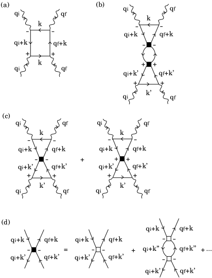
Figure 2: Diagrams within the ladder approximation. Panels (a) amd (b) are the diagrams of the lowest-order and the higher-order, respectively, in the Coulomb interaction. Panel(c) is the diagram where the renormalized vertex works only at the outward time leg and at the backward time leg, respectively. Panel (d) represents the renormalized vertex which is the sum of the ladder diagrams. The horizontal and vertical solid lines represent the Green’s functions of the 2p-core and $d$ electrons, respectively. The filled squares represent the renormalized vertex. The symbols $-$ and $+$ indicate the outward and backward time legs, respectively.

Second, we consider the diagram shown in Fig. 2(b). The solid square represents the renormalized vertex function, which we evaluate by collecting up the ladder diagrams. Then, carrying out the integration with respect to the frequency of the 2p Green’s function, we obtain the contribution to the RIXS intensity as

$$W_{b}(\omega_{i},q;\alpha_{i},\alpha_{f})$$ (27)

$$= \hat{M}^{\dagger}(\alpha_{i},\alpha_{f})\hat{L}^{\dagger}(\omega_{i},q)\hat{\Gamma}\left[\hat{I}+\hat{F}^{\dagger}(q)\hat{\Gamma}\right]^{-1}\hat{\Pi}^{(0)}(q)$$

$$\times \left[\hat{I}+\hat{\Gamma}\hat{F}(q)\right]^{-1}\hat{\Gamma}\hat{L}(\omega_{i},q)\hat{M}(\alpha_{i},\alpha_{f}),$$

where each factors are given in the matrix form represented with the base states $\xi\xi^{\prime}$. The $\hat{M}$ is the matrix form of Eq. (LABEL:eq.M):

$$\left[\hat{M}(\alpha_{i},\alpha_{f})\right]_{\xi\xi^{\prime}}=M(\xi\xi^{\prime};\alpha_{i},\alpha_{f}).$$ (28)

The $\hat{L}$ corresponds to the diagram above the renormalized vertex on Fig. 2(b):

$$\left[\hat{L}(\omega_{i},q)\right]_{\xi_{1}\xi^{\prime}_{1};\xi\xi^{\prime}}=\frac{2}{N}\sum_{{\bf k}}\sum_{j,\ell}U_{\xi_{1}j}({\bf k+q})U^{*}_{\xi j}({\bf k+q})U_{\xi^{\prime}\ell}({\bf k})U^{*}_{\xi^{\prime}_{1}\ell}({\bf k})R(\omega_{i},E_{j}({\bf k+q}))$$ (29)

$$\times \Biggl{\{}\frac{1-n_{\ell}({\bf k})}{\omega_{f}-E_{\ell}({\bf k})+\epsilon_{2p}(3/2)+i\Gamma_{c}}-\Biggl{[}\frac{[1-n_{j}({\bf k+q})]n_{\ell}({\bf k})}{\omega-E_{j}({\bf k+q})+E_{\ell}({\bf k})+i\delta}-\frac{n_{j}({\bf k+q})[1-n_{\ell}({\bf k})]}{\omega-E_{j}({\bf k+q})+E_{\ell}({\bf k})-i\delta}\Biggr{]}\Biggr{\}}.$$

We get a complicated form for $\hat{L}(\omega_{i};q)$, since the creation and annihilation of $d$ electron take place at different times. For understanding the origin of each term, it may be helpful to carry out the integration in the time representation (See Appendix A). Vertex $\hat{\Gamma}$ is defined by

$$[\hat{\Gamma}]_{\xi_{2}\xi^{\prime}_{2};\xi_{1}\xi^{\prime}_{1}}=\Gamma^{(0)}(\xi_{2}\xi^{\prime}_{1};\xi_{1}\xi^{\prime}_{2}).$$ (30)

The $\hat{F}(q)$ is given by

$$[\hat{F}(q)]_{\xi_{2}\xi^{\prime}_{2};\xi_{1}\xi^{\prime}_{1}} = -i\frac{2}{N}\sum_{{\bf k}}\int\frac{{\rm d}k_{0}}{2\pi}[\hat{G}({\bf k+q},k_{0}+\omega)]_{\xi_{2}\xi_{1}}[\hat{G}({\bf k},k_{0})]_{\xi^{\prime}_{1}\xi^{\prime}_{2}}$$ (31)

$$= \frac{2}{N}\sum_{{\bf k}}\sum_{j,\ell}U_{\xi_{2}j}({\bf k+q})U_{\xi_{1}j}^{*}({\bf k+q})U_{\xi^{\prime}_{1}\ell}({\bf k})U_{\xi^{\prime}_{2}\ell}^{*}({\bf k})$$

$$\times \left[\frac{[1-n_{j}({\bf k+q})]n_{\ell}({\bf k})}{\omega-E_{j}({\bf k+q})+E_{\ell}({\bf k})+i\delta}-\frac{n_{j}({\bf k+q})[1-n_{\ell}({\bf k})]}{\omega-E_{j}({\bf k+q})+E_{\ell}({\bf k})-i\delta}\right],$$

which is a conventional particle-hole propagator. Note that the factors $[\hat{I}+\hat{\Gamma}\hat{F}(q)]^{-1}\hat{\Gamma}$ and $\hat{\Gamma}[\hat{I}+\hat{F}^{\dagger}(q)\hat{\Gamma}]^{-1}$ are the renormalized vertices within the ladder approximation, which could contain a pole at some $q$, as the indication of the bound state. As shown in the next subsection, the bound state could surely contribute to the RIXS intensity. The $\hat{\Pi}^{(0)}$ corresponds to the diagram between two renormalized vertices on Fig. 2(b):

$$\left[\hat{\Pi}^{(0)}(q)\right]_{\xi_{2}\xi^{\prime}_{2};\xi_{1}\xi^{\prime}_{1}} = 2\pi\frac{2}{N}\sum_{{\bf k}}\sum_{j,\ell}U_{\xi_{2}j}({\bf k+q})U_{\xi_{1}j}^{*}({\bf k+q})U_{\xi^{\prime}_{1}\ell}({\bf k})U_{\xi^{\prime}_{2}\ell}^{*}({\bf k})$$ (32)

$$\times [1-n_{j}({\bf k+q})]n_{\ell}({\bf k})\delta(\omega-E_{j}({\bf k+q})+E_{\ell}({\bf k})).$$

To complete the ladder approximation, we need to include another type of diagrams shown in Fig. 2(c). Carrying out the integration with respect to the frequency of the 2p Green’s function, we obtain the contribution from the diagrams in Fig. 2(c):

$$W_{c}(\omega_{i},q;\alpha_{i},\alpha_{f}) = \hat{M}^{\dagger}(\alpha_{i},\alpha_{f})\Bigl{\{}\hat{N}^{\dagger}(\omega_{i},q)[\hat{I}+\hat{\Gamma}\hat{F}(q)]^{-1}\hat{\Gamma}\hat{L}(\omega_{i},q)$$ (33)

$$+ \hat{L}^{\dagger}(\omega_{i},q)\hat{\Gamma}[\hat{I}+\hat{F}^{\dagger}(q)\hat{\Gamma}]^{-1}\hat{N}(\omega_{i},q)\Bigr{\}}\hat{M}(\alpha_{i},\alpha_{f}).$$

The $\hat{N}$ corresponds to the diagram above the renormalized vertex on the right-hand side of Fig. 2(c):

$$\left[\hat{N}(\omega_{i},q)\right]_{\xi_{1}\xi^{\prime}_{1};\xi\xi^{\prime}} = 2\pi\frac{2}{N}\sum_{{\bf k}}\sum_{j,\ell}U_{\xi_{1}j}({\bf k+q})U^{*}_{\xi j}({\bf k+q})U_{\xi^{\prime}\ell}({\bf k})U^{*}_{\xi^{\prime}_{1}\ell}({\bf k})R(\omega_{i},E_{j}({\bf k+q}))$$ (34)

$$\times [1-n_{j}({\bf k+q})]n_{\ell}({\bf k})\delta(\omega-E_{j}({\bf k+q})+E_{\ell}({\bf k})).$$

Note that the pole in $[\hat{I}+\hat{F}^{\dagger}(q)\hat{\Gamma}]^{-1}$ and $[\hat{I}+\hat{\Gamma}\hat{F}(q)]^{-1}$ in Eq. (33) could not contribute to the RIXS intensity because of $\delta(\omega-E_{j}({\bf k+q})+E_{\ell}({\bf k}))$ in Eq. (34).

The total RIXS intensity is given by $W_{a}(\omega_{i},q;\alpha_{i},\alpha_{f})+W_{b}(\omega_{i},q;\alpha_{i},\alpha_{f})+W_{c}(\omega_{i},q;\alpha_{i},\alpha_{f})$.

III.4 Correlation function and bound state

The contribution from the diagram of type (b) in Fig. 2 may be rewritten as

$$W_{b}(\omega_{i},q;\alpha_{i},\alpha_{f}) = \hat{M}^{\dagger}(\alpha_{i},\alpha_{f})\hat{L}^{\dagger}(\omega_{i},q)\hat{\Gamma}\hat{Y}^{+-}(q)$$ (35)

$$\times \hat{\Gamma}\hat{L}(\omega_{i},q)\hat{M}(\alpha_{i},\alpha_{f}),$$

where

$$\left[\hat{Y}^{+-}({\bf q},\omega)\right]_{\xi_{1}\xi^{\prime}_{1};\xi\xi^{\prime}}=\int_{-\infty}^{\infty}\langle(\rho_{{\bf q}\xi_{1}\xi^{\prime}_{1}}(t))^{\dagger}\rho_{{\bf q}\xi\xi^{\prime}}(0)\rangle{\rm e}^{i\omega t}{\rm d}t,$$ (36)

with

$$\rho_{{\bf q}\xi\xi^{\prime}}=\sqrt{\frac{2}{N}}\sum_{\bf k}a_{\xi}^{\dagger}({\bf k+q})a_{\xi^{\prime}}({\bf k}).$$ (37)

Function $\hat{Y}^{+-}({\bf q},\omega)$, connecting the outward and backward time legs, is nothing but a density-density correlation function in the equilibrium state. Note that the factor $\hat{\Gamma}\hat{L}(\omega_{i},q)\hat{M}(\alpha_{i},\alpha_{f})$ may be regarded as an effective transition amplitude creating an electron-hole pair.

In order to prove Eq. (35), we introduce the time-ordered Green’s function in the Feynman-Dyson scheme,

$$\left[\hat{Y}^{{\rm T}}(q)\right]_{\xi_{1}\xi^{\prime}_{1};\xi\xi^{\prime}}=-i\int\langle T[(\rho_{{\bf q}\xi_{1}\xi^{\prime}_{1}}(t))^{\dagger}\rho_{{\bf q}\xi\xi^{\prime}}(0)]\rangle{\rm e}^{i\omega t}{\rm d}t,$$ (38)

where the time-ordering is defined in the outward time leg. This function is related to the correlation function by using a modified form of the fluctuation-dissipation theorem for $\omega>0$ (see Appendix B):

$$\left[\hat{Y}^{+-}(q)\right]_{\xi_{1}\xi^{\prime}_{1};\xi\xi^{\prime}}=-i\left\{\left[\hat{Y}^{{\rm T}}(q)\right]^{*}_{\xi\xi^{\prime};\xi_{1}\xi^{\prime}_{1}}-\left[\hat{Y}^{{\rm T}}(q)\right]_{\xi_{1}\xi^{\prime}_{1};\xi\xi^{\prime}}\right\}.$$ (39)

Within the ladder approximation in the Feynman-Dyson scheme, $\hat{Y}^{T}(q)$ is expressed as

$$\hat{Y}^{{\rm T}}(q)=\hat{F}(q)[\hat{I}+\hat{\Gamma}\hat{F}(q)]^{-1}.$$ (40)

Using a relation $1/(\omega-E\pm i\delta)=P\{1/(\omega-E)\}\mp i\pi\delta(\omega-E)$ in the last line of Eq. (31), we express $\hat{F}(q)$ as

$$\hat{F}(q)=\hat{F}_{1}(q)+i\hat{F}_{2}(q),$$ (41)

where $\hat{F}_{1}(q)$ and $\hat{F}_{2}(q)$ are Hermitian matrices. Using this Hermitian property and the fact that $\hat{\Gamma}$ is a real and symmetric matrix, we find a relation

$$\left[\hat{Y}^{{\rm T}}(q)\right]^{*}_{\xi\xi^{\prime};\xi_{1}\xi^{\prime}_{1}}$$

$$= \left\{[\hat{I}+(\hat{F}_{1}(q)-i\hat{F}_{2}(q))\hat{\Gamma}]^{-1}(\hat{F}_{1}(q)-i\hat{F}_{2}(q))\right\}_{\xi_{1}\xi^{\prime}_{1};\xi\xi^{\prime}},$$

and hence

$$\left[\hat{Y}^{+-}(q)\right]_{\xi_{1}\xi^{\prime}_{1};\xi\xi^{\prime}}$$

$$= -i\left\{\left[\hat{Y}^{{\rm T}}(q)\right]^{*}_{\xi\xi^{\prime};\xi_{1}\xi^{\prime}_{1}}-\left[\hat{Y}^{{\rm T}}(q)\right]_{\xi_{1}\xi^{\prime}_{1};\xi\xi^{\prime}}\right\}$$

$$= \Bigl{\{}[\hat{I}+(\hat{F}(q))^{\dagger}\hat{\Gamma}]^{-1}(-2)\hat{F}_{2}(q)[\hat{I}+\hat{\Gamma}\hat{F}(q)]^{-1}\Bigr{\}}_{\xi_{1}\xi^{\prime}_{1};\xi\xi^{\prime}}.$$

Since $-2\hat{F}_{2}(q)$ is equivalent to $\hat{\Pi}^{(0)}(q)$, we see Eq. (35) is equivalent to Eq. (27).

Now we discuss the bound state. The Green’s function given by Eq. (40) may have poles for some frequencies below the energy continuum of an electron-hole pair excitation. In the antiferromagetic ground state, for example, such bound states are known as “magnon”, which give rise to extra RIXS intensities. Noting that $\hat{F}_{2}(q)=0$ for $\omega$ below the energy continuum, Eq. (40) is rewritten as

$$\hat{Y}^{{\rm T}}(q)=\left[\hat{F}_{1}(q)^{-1}+\hat{\Gamma}\right]^{-1}.$$ (44)

Diagonalizing $\hat{F}_{1}(q)^{-1}+\hat{\Gamma}$ by a unitary matrix, we assume that one eigenvalue becomes zero at $\omega=\omega_{B}({\bf q})$ with the eigenvector $B_{\xi_{2}\xi^{\prime}_{2}}({\bf q})$. We could expand $[\hat{Y}^{{\rm T}}(q)]_{\xi_{1}\xi^{\prime}_{1};\xi\xi^{\prime}}$ around $\omega\sim\omega_{B}({\bf q})$ as

$$\left[\hat{Y}^{{\rm T}}(q)\right]_{\xi_{1}\xi^{\prime}_{1};\xi\xi^{\prime}}=\frac{[\hat{C}({\bf q})]_{\xi_{1}\xi^{\prime}_{1};\xi\xi^{\prime}}}{\omega-\omega_{B}({\bf q})+i\delta},$$ (45)

with

$$[\hat{C}({\bf q})]_{\xi_{1}\xi^{\prime}_{1};\xi\xi^{\prime}}=\frac{B_{\xi_{1}\xi^{\prime}_{1}}({\bf q})B_{\xi\xi^{\prime}}^{*}({\bf q})}{\sum_{\xi_{2}\xi^{\prime}_{2}\xi_{3}\xi^{\prime}_{3}}B_{\xi_{3}\xi^{\prime}_{3}}^{*}({\bf q})\frac{\partial}{\partial\omega}[\hat{F}_{1}({\bf q},\omega_{B}({\bf q}))^{-1}]_{\xi_{3}\xi^{\prime}_{3};\xi_{2}\xi^{\prime}_{2}}B_{\xi_{2}\xi^{\prime}_{2}}({\bf q})}.$$ (46)

Substituting Eq. (45) into the right hand side of Eq. (39), we obtain

$$\hat{Y}^{+-}(q)=2\pi\hat{C}({\bf q})\delta(\omega-\omega_{B}({\bf q})).$$ (47)

Inserting this result into Eq. (35), we have the contribution from the bound state.

III.5 Fast collision approximation

The RIXS spectra could be described as the second-order dipole allowed process. For that process the fast collision approximation replaces the intermediate state by a single state. In the context of the present theory, this means that $E_{j}({\bf k+q})$ is replaced by a certain energy $E_{0}$ in the denominator of Eq. (24), and that factor is decoupled from the others. Hence, we have

$$W_{a}(\omega_{i},q;\alpha_{i},\alpha_{f})=\left|R(\omega_{i},E_{0})\right|^{2}\hat{M}^{\dagger}(\alpha_{i},\alpha_{f})\hat{\Pi}^{(0)}(q)\hat{M}(\alpha_{i},\alpha_{f}).$$ (48)

In addition, we disregard the first term in Eq. (29), and make the same decoupling procedure to the second term. Hence we have for $\hat{L}(\omega_{i},q)$,

$$\hat{L}(\omega_{i},q)=-R(\omega_{i},E_{0})\hat{F}(q).$$ (49)

In the same spirit, we can approximate $\hat{N}(\omega_{i},q)$ by

$$\hat{N}(\omega_{i},q)=R(\omega_{i},E_{0})\hat{\Pi}^{(0)}(q).$$ (50)

With these approximate expressions, we have the total RIXS intensity as

$$W_{a}(\omega_{i},q;\alpha_{i},\alpha_{f})+W_{b}(\omega_{i},q;\alpha_{i},\alpha_{f})+W_{c}(\omega_{i},q;\alpha_{i},\alpha_{f})$$ (51)

$$= \left|R(\omega_{i},E_{0})\right|^{2}\hat{M}^{\dagger}(\alpha_{i},\alpha_{f})\left[\hat{I}+\hat{F}^{\dagger}(q)\right.$$

$$\times \left.\hat{\Gamma}\right]^{-1}\hat{\Pi}^{(0)}(q)\left[\hat{I}+\hat{\Gamma}\hat{F}(q)\right]^{-1}\hat{M}(\alpha_{i},\alpha_{f})$$

$$= \left|R(\omega_{i},E_{0})\right|^{2}\hat{M}^{\dagger}(\alpha_{i},\alpha_{f})Y^{+-}(q)\hat{M}(\alpha_{i},\alpha_{f}).$$

In the situation that $E_{j}({\bf k+q})$ varies considerably depending on $j$ and ${\bf k+q}$, the procedure made above seems difficult to be justified.

IV Application to the single-orbital Hubbard model on the square lattice

We have obtained the formulas of the $L$-edge RIXS spectra for multi-orbital models. Since they are rather complicated, we demonstrate in the following how the formulas work through the application to a simple model, a single-orbital Hubbard model with nearest-neighbor hopping on the square lattice at half-filling. The Hamiltonian is defined by

$$H_{\rm mat}=\sum_{\sigma}\sum_{i,j}t_{ij}a_{i\sigma}^{\dagger}a_{j\sigma}+U\sum_{i}a_{i\uparrow}^{\dagger}a_{i\downarrow}^{\dagger}a_{i\downarrow}a_{i\uparrow}.$$ (52)

IV.1 HFA to the single-particle states

The antiferromagetic ordering is known to be realized in the ground state. Specifying the sublattices by A and B, we put the base states $\xi$’s in order ($A,\uparrow$), ($B,\uparrow$), ($A,\downarrow$), and ($B,\downarrow$). Then $\hat{J}({\bf k})$ is represented as

$$\hat{J}({\bf k})=\left(\begin{array}[]{cccc}-Um&\epsilon_{\bf k}&0&0\\ \epsilon_{\bf k}&Um&0&0\\ 0&0&Um&\epsilon_{\bf k}\\ 0&0&\epsilon_{\bf k}&-Um\end{array}\right),$$ (53)

where

$$\epsilon_{\bf k} = -2t(\cos k_{x}+\cos k_{y}),$$ (54)

$$m = \frac{1}{2}\langle a_{i\uparrow}^{\dagger}a_{i\uparrow}-a_{i\downarrow}^{\dagger}a_{i\downarrow}\rangle,\quad{\rm for}\,\,i\in A.$$ (55)

Matrix $\hat{J}({\bf k})$ is diagonalized by a unitary matrix

$$\hat{U}({\bf k})=\left(\begin{array}[]{cccc}\cos\theta_{\bf k}&-\sin\theta_{\bf k}&0&0\\ \sin\theta_{\bf k}&\cos\theta_{\bf k}&0&0\\ 0&0&\cos\theta_{\bf k}&\sin\theta_{\bf k}\\ 0&0&-\sin\theta_{\bf k}&\cos\theta_{\bf k}\end{array}\right),$$ (56)

where the corresponding eigenvalues are $-E({\bf k})$, $E({\bf k})$, $E({\bf k})$, and $-E({\bf k})$ with $E({\bf k})=\sqrt{\epsilon_{\bf k}^{2}+(Um)^{2}}$, and $\theta_{\bf k}$ is determined from

$$\tan 2\theta_{\bf k}=-\frac{\epsilon_{\bf k}}{Um}.$$ (57)

The sublattice magnetization $m$ is self-consistently determined by

$$1=U\frac{2}{N}\sum_{\bf k}\frac{1}{2E({\bf k})}.$$ (58)

For $U/t=4$ and $2$, $m$ is evaluated as $0.345$ and $0.188$, respectively.

IV.2 Absorption coefficient

X-ray could be absorbed by exciting the $2p$ electron to unoccupied levels at the $L$ edge. Neglecting the interaction between the excited electron and the core hole left behind, we obtain the expression of the absorption coefficient at the $L_{3}$ edge as

$$A(\omega_{i})\propto-\frac{2}{N}\sum_{\bf k}\frac{1}{\pi}\textrm{Im}[R(\omega_{i},E(\textbf{k}))],$$ (59)

where $\textrm{Im}X$ stands for the imaginary part of the quantity $X$. Figure 3 shows the absorption coefficient $A(\omega_{i})$ as a function of x-ray energy for $U/t=4$ and $2$. We set $\Gamma_{c}/t=0.3$. The absorption peak is found at $\omega_{i}/t=1.51$ for $U/t=4$ and $\omega_{i}/t=0.55$ for $U/t=2$ where $\omega_{i}$ is measured from $\mu-\epsilon_{2p}(3/2)$.

Figure 3: Absorption coefficient $A(\omega_{i})$ as a function of x-ray energy, for $U/t=4$ (solid line) and 2 (broken line). $\Gamma_{c}/t=0.3$. The origin of energy is $\mu-\epsilon_{2p}(3/2)$, where $\mu$ is the chemical potential lying at the middle of the energy gap in the single particle energy band. The solid and broken arrows indicate the lowest bound of energy of unoccupied levels for $U/t=4$ and 2, respectively.

IV.3 RIXS spectra

The transverse spin fluctuation caused by spin flips with changing polarization of x-ray contains the magnon as a bound state, while the longitudinal spin fluctuation caused without changing polarization could not give rise to the bound state. Since we are interested in the relation between the spectra arising from the bound state and the continuum states, we confine our study to the spin flip channel in the following.

Bearing a relation to cuprates in mind, we assume that the orbital describing the Hubbard model is $3d_{x^{2}-y^{2}}$. In that situation, $M(\xi\xi^{\prime};\alpha_{i},\alpha_{f})$ is the same as that given in the study of magnetic excitations in the L-edge RIXS from cuprates (Table II in Ref. Igarashi and Nagao, 2012a.). With the spin quantization axis lying on the $xy$ plane and pointing to the direction at angle $\gamma$ with the $x$ axis, it is given by

$$M(-\sigma\sigma;y,x)=-M(-\sigma\sigma;x,y)=\frac{i}{15}{\rm e}^{i\sigma\gamma}w^{2},$$ (60)

where $w$ is a constant, and $\sigma=+1$ ($-1$) indicates the up (down) spin. When $\alpha_{i}$ and $\alpha_{f}$ are specified as $x$ or $y$, they are pointing to the $x$ or $y$, axes. Note that $M(\xi\xi^{\prime};\alpha_{i},\alpha_{f})$ has no sublattice dependence.

In the spin flip channel, there exist two channels $c_{1}$ and $c_{2}$, represented by the base states $(\xi\xi^{\prime})=(A\uparrow A\downarrow)$, $=(B\uparrow B\downarrow)$, called channel $c_{1}$, and by the base states $(B\downarrow B\uparrow)$, $(A\downarrow A\uparrow)$, called channel $c_{2}$. In both channels, we have

$$\hat{M}(y,x) = -\hat{M}(x,y)=\frac{i}{15}w^{2}{\rm e}^{i\sigma\gamma}\left(\begin{array}[]{c}1\\ 1\end{array}\right),$$ (63)

$$\hat{\Gamma} = \left(\begin{array}[]{cc}U&0\\ 0&U\end{array}\right).$$ (66)

It is clear that both channels give rise to the same contributions to the RIXS intensities.

We calculate the RIXS spectra by following the procedure in the preceding section. In channel $c_{1}$, for example, the zero-th order of the particle-hole Green’s function is written as

$$\hat{F}({\bf q},\omega) = \frac{2}{N}\sum_{\bf k}\frac{1}{\omega-E({\bf k+q})-E({\bf k})+i\delta}$$

$$\times \left(\begin{array}[]{cc}\sin^{2}\theta_{\bf k+q}\sin^{2}\theta_{\bf k}&-\frac{1}{4}\sin 2\theta_{\bf k+q}\sin 2\theta_{\bf k}\\ -\frac{1}{4}\sin 2\theta_{\bf k+q}\sin 2\theta_{\bf k}&\cos^{2}\theta_{\bf k+q}\cos^{2}\theta_{\bf k}\end{array}\right)$$

$$- \frac{2}{N}\sum_{\bf k}\frac{1}{\omega+E({\bf k+q})+E({\bf k})-i\delta}$$

$$\times \left(\begin{array}[]{cc}\cos^{2}\theta_{\bf k+q}\cos^{2}\theta_{\bf k}&-\frac{1}{4}\sin 2\theta_{\bf k+q}\sin 2\theta_{\bf k}\\ -\frac{1}{4}\sin 2\theta_{\bf k+q}\sin 2\theta_{\bf k}&\sin^{2}\theta_{\bf k+q}\sin^{2}\theta_{\bf k}\end{array}\right).$$ (72)

The particle-hole Green’s function is given by $\hat{Y}^{T}({\bf q},\omega)=\hat{F}({\bf q},\omega)[\hat{I}+\hat{\Gamma}\hat{F}({\bf q},\omega)]^{-1}$.

There exists a bound state below the energy continuum ($\omega<2Um$). The energy of the bound state should tend to $0$ with ${\bf q}\rightarrow 0$, since it is a Goldstone boson. This is proved as follows. Let $\hat{F}({\bf q},\omega)$ be

$$\hat{F}({\bf q}\rightarrow 0,\omega\rightarrow 0)=\left(\begin{array}[]{cc}f_{1}&f_{2}\\ f_{2}&f_{1}\end{array}\right).$$ (74)

Then the particle-hole Green’s function is given by

$$\hat{Y}^{T}({\bf q}\rightarrow 0,\omega\rightarrow 0)=\hat{S}\left(\begin{array}[]{cc}\frac{f_{1}+f_{2}}{1+U(f_{1}+f_{2})}&0\\ 0&\frac{f_{1}-f_{2}}{1+U(f_{1}-f_{2})}\end{array}\right)\hat{S}^{-1},$$ (75)

where

$$\hat{S}=\frac{1}{\sqrt{2}}\left(\begin{array}[]{cc}1&-1\\ 1&1\\ \end{array}\right).$$ (76)

Since

$$f_{1}-f_{2}=-\frac{2}{N}\sum_{\bf k}\frac{(\sin^{2}\theta_{\bf k}+\cos^{2}\theta_{\bf k})^{2}}{2E_{\bf k}}=-\frac{2}{N}\sum_{\bf k}\frac{1}{2E_{\bf k}},$$ (77)

we have $1+U(f_{1}-f_{2})=0$ from Eq. (58), indicating that a pole exist at ${\bf q}=0$ and $\omega=0$. In addition, we find from Eq. (46) that

$$\hat{C}({\bf q}\rightarrow 0)\propto\left(\begin{array}[]{cc}\frac{1}{2}&-\frac{1}{2}\\ -\frac{1}{2}&\frac{1}{2}\end{array}\right).$$ (78)

In the fast collision approximation, the contribution to the RIXS intensity from the bound state vanishes with ${\bf q}\rightarrow 0$, since $\hat{M}^{\dagger}\hat{C}\hat{M}=0$. Beyond the fast collision approximation, however, it does not vanish due to the presence of $\hat{L}(\omega_{i},q)$.

In the numerical calculation, we sum over wave vectors by dividing the first magnetic BZ into $128\times 128$ meshes. Figure 4 shows the RIXS spectra as a function of $\omega$ along a symmetry line of ${\bf q}\parallel(1,0)$. The energy of the incident x-ray $\omega_{i}$ is set to give the maximum absorption coefficient. We have the continuous spectra for $\omega>2Um$, and below them we find $\delta$-function-like spikes arising from the magnon contribution. For $U/t=4$, the magnon peak arising exists for all the $q$-values. Around ${\bf q}=0$, the velocity of magnon $\omega/|{\bf q}|$ is estimated as $\sim 0.8$ in units of $t$, which may be compared by $\sqrt{2}J$ with $J=4t^{2}/U$ for the localized spin limit. The intensity of the magnon peak decreases with increasing value of $|{\bf q}|$; its value relative to the intensity of continuous states at $(\pi,0)$ is estimated as $0.175$ for $(\pi/8,0)$, $0.120$ for $(\pi/2,0)$, and $0.08$ for $(\pi,0)$. For $U/t=2$, the magnon mode approaches to the edge of the continuous spectra with increasing $|{\bf q}|$, and it becomes difficult to judge numerically whether the magnon peak exists for $q_{x}>\pi/2$. The intensity of the magnon peak relative to the intensity of continuous states at $(\pi,0)$ is estimated as 0.27 for $(\pi/8,0)$ and 0.10 for $(\pi/2,0)$.

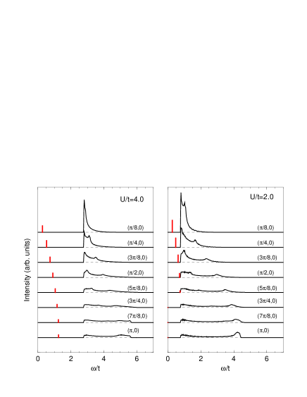
Figure 4: (Color Online) RIXS spectra as a function of energy loss $\omega$ for the single-orbital Hubbard model on the square lattice at half-filling along a symmetry line ${\bf q}\parallel(1,0)$. $\Gamma_{c}/t=0.3$. The incident x-ray energy $\omega_{i}$ is set to give the maximum absorption coefficient; $\omega_{i}/t=1.51$ for $U/t=4$, and $\omega_{i}/t=0.55$ for $U/t=2$ with $\omega_{i}$ measured from $\mu-\epsilon_{2p}(3/2)$. Solid vertical line (red) indicates the magnon contribution.

V Concluding remarks

We have developed a formalism of the $L$-edge RIXS spectra on a multi-orbital tight-binding model. Without relying on the fast collision approximation, we have derived the formulas useful to calculate the spectra, by collecting up the ladder diagrams on the basis of the Keldysh scheme. Since the creation of an electron and that of a hole take place at different times, the formulas become complicated in comparison with the fast collision approximation. We think that, the present formulas, allowing to describe the spectra originated from both the bound state and the continuous states on the equal footing, work in the weak and intermediate coupling regime of itinerant electron systems, where the fast collision approximation loses ground with several orbitals involved with different energies. To demonstrate how the present formulas work, we have calculated the spectra on a simple model, the single-orbital Hubbard model on the square lattice at half-filling. Now we know they work, it may be interesting to apply the present formulas to analyze the spectra of Sr₂IrO₄ on the itinerant electron model, although the analysis has already been carried out on the localized electron model within the fast collision approximation.Ament et al. (2011b)

In the insulating phase of the strong coupling regime, the low-lying excitations may be described by the localized spin and/or orbital model. In undoped cuptares, using the Heisenberg model, the RIXS spectra arising from magnetic excitations have been calculated within the fast collision approximationAment et al. (2009); Haverkort (2010) and with using a “projection” method to take account of the two-magnon excitations.Igarashi and Nagao (2012a, b); Nagao and Igarashi (2012) The present approximation scheme is unable to discuss such behavior in the strong coupling. To deal with the metallic phase with strong correlations, the present formalism for itinerant electron systems has to be extended by improving the HFA and the ladder approximation. In that extension, the single-particle Green’s function is corrected by the self-energy, and hence the present formulas may be changed by noting that the Green’s function within the HFA

$$[\hat{G}({\bf k},\omega)]_{\xi_{2}\xi_{1}}=\sum_{j}\frac{U_{\xi_{2}j}({\bf k})U_{\xi_{1}j}^{*}({\bf k})}{\omega-E_{j}({\bf k})+i\delta{\rm sgn}[E_{j}({\bf k})]}$$ (79)

is formally replaced by

$$[\hat{G}({\bf k},\omega)]_{\xi_{2}\xi_{1}}=\int{\rm d}\epsilon\frac{\rho_{\xi_{2}\xi_{1}}({\bf k},\epsilon)}{\omega-\epsilon+i\delta{\rm sgn}[\epsilon]}.$$ (80)

Such attempt may be related to the recent study on the RIXS spectra in the Falicov-Kimball model on the basis of the Keldysh scheme, Pakhira et al. (2012) where the dynamical mean field approximation is used.

Appendix A Derivation of Eq. (29) in the time representation

Let us consider a diagram in Fig. 5 written in the time representation. The corresponding amplitude may be proportional to

$$\hat{L}(\omega_{i};{\bf q},s) \propto \int_{-\infty}^{0}{\rm d}tiG_{2p}^{--}({\bf k-q}_{f},t-0)iG^{--}({\bf k+q},s-t)$$ (81)

$$\times iG^{--}({\bf k},0-s)\exp(-i\omega_{i}t),$$

where the factors $U_{\xi_{1}j}({\bf k+q})U^{*}_{\xi j}({\bf k+q})$ $U_{\xi^{\prime}\ell}({\bf k})U^{*}_{\xi^{\prime}_{1}\ell}({\bf k})$, and the symbol of summing over ${\bf k}$ are omitted in this subsection. The $\hat{L}(\omega_{i};{\bf q},s)$ is the Fourier transform of $\hat{L}(\omega_{i},q=(\omega,{\bf q}))$. Since $t<0$, we have

$$iG_{2p}^{--}({\bf k-q}_{f},t-0)=-\exp\{-i(\epsilon_{2p}(3/2)+i\Gamma_{c})t\}.$$ (82)

First we consider the time domain $s>0$. The Green’s functions are given by

$$iG^{--}({\bf k},0-s) = -\sum_{\ell}n_{\ell}({\bf k})\textrm{e}^{-iE_{\ell}({\bf k})(-s)},$$ (83)

$$iG^{--}({\bf k+q},s-t) = \sum_{j}(1-n_{j}({\bf k+q}))\textrm{e}^{-iE_{j}({\bf k+q})(s-t)}.$$

Inserting these into Eq. (81), we have

$$\hat{L}(\omega_{i};{\bf q},s) \propto -\frac{1}{i}R(\omega_{i},E_{j}({\bf k+q}))(1-n_{j}({\bf k+q}))n_{\ell}({\bf k})$$ (85)

$$\times \exp\{-i(E_{j}({\bf k+q})-E_{\ell}({\bf k}))s\}.$$

The Fourier transform of this function corresponds to the former part of the second term of Eq. (29).

Next we consider the time domain $s<0$. The Green’s functions are given by

$$iG^{--}({\bf k},0-s) = \sum_{\ell}(1-n_{\ell}({\bf k}))\textrm{e}^{-iE_{\ell}({\bf k})(-s)},$$ (86)

$$iG^{--}({\bf k+q},s-t) = \left\{\begin{array}[]{ll}-\sum_{j}n_{j}({\bf k+q})\textrm{e}^{-iE_{j}({\bf k+q})(s-t)},&s<t,\\ \sum_{j}(1-n_{j}({\bf k+q}))\textrm{e}^{-iE_{j}({\bf k+q})(s-t)},&t<s<0.\end{array}\right.$$ (89)

Inserting these into Eq. (81), we have

$$\hat{L}(\omega_{i};{\bf q},s) \propto -\frac{1}{i}R(\omega_{i},E_{j}({\bf k+q}))\Bigl{\{}n_{j}({\bf k+q}))(1-n_{\ell}({\bf k}))\exp\{-i(E_{j}({\bf k+q})-E_{\ell}({\bf k}))s\}$$ (90)

$$- (1-n_{\ell}({\bf k}))\exp\{-i(\omega_{i}+\epsilon_{2p}(3/2)+i\Gamma_{c}-E_{\ell}({\bf k}))s\}\Bigr{\}}.$$

The Fourier transform of the first term corresponds to the first term of Eq. (29), and that of the second term corresponds to the latter part of the second term of Eq. (29).

Figure 5: Diagram for $\hat{L}(\omega_{i};{\bf q},s)$ in the time representation. The $s$ is the time at which the Coulomb interaction works.

Appendix B Derivation of Eq. (39)

Let $\hat{A}_{1}$ and $\hat{A}_{2}$ be $\rho_{{\bf q}\xi_{1}\xi^{\prime}_{1}}$ and $\rho_{{\bf q}\xi\xi^{\prime}}$, respectively. Then we have

$$\left[\hat{Y}^{T}(\omega)\right]_{1,2} \equiv -i\int_{-\infty}^{\infty}\langle T(A_{1}^{\dagger}(t)A_{2}(0))\rangle{\rm e}^{i\omega t}{\rm d}t$$ (91)

$$= \sum_{n}\frac{\langle 0|A_{1}^{\dagger}|n\rangle\langle n|A_{2}|0\rangle}{\omega-E_{n}+E_{0}+i\delta}$$

$$- \sum_{n}\frac{\langle 0|A_{2}|n\rangle\langle n|A_{1}^{\dagger}|0\rangle}{\omega+E_{n}-E_{0}-i\delta},$$

$$\left[\hat{Y}^{T}(\omega)\right]^{*}_{2,1} = \sum_{n}\frac{\langle 0|A_{1}^{\dagger}|n\rangle\langle n|A_{2}|0\rangle}{\omega-E_{n}+E_{0}-i\delta}$$ (92)

$$- \sum_{n}\frac{\langle 0|A_{2}|n\rangle\langle n|A_{1}^{\dagger}|0\rangle}{\omega+E_{n}-E_{0}+i\delta},$$

where $|0\rangle$ and $|n\rangle$ denote the ground state with energy $E_{0}$ and the excited state with energy $E_{n}$, respectively. Hence we have

$$\left[\hat{Y}^{T}(\omega)\right]^{*}_{2,1}-\left[\hat{Y}^{T}(\omega)\right]_{1,2}$$ (93)

$$= 2\pi i\sum_{n}\langle 0|A_{1}^{\dagger}|n\rangle\langle n|A_{2}|0\rangle\delta(\omega-E_{n}+E_{0})$$

$$+ 2\pi i\sum_{n}\langle 0|A_{2}|n\rangle\langle n|A_{1}^{\dagger}|0\rangle\delta(\omega+E_{n}-E_{0}).$$

Comparing this with the expression

$$\left[\hat{Y}^{+-}(\omega)\right]_{1,2} \equiv \int_{-\infty}^{\infty}\langle A_{1}^{\dagger}(t)A_{2}(0)\rangle{\rm e}^{i\omega t}{\rm d}t$$

$$= 2\pi\sum_{n}\langle 0|A_{1}^{\dagger}|n\rangle\langle n|A_{2}|0\rangle\delta(\omega-E_{n}+E_{0}),$$

we have $[\hat{Y}^{+-}(\omega)]_{1,2}=-i\{[\hat{Y}^{T}(\omega)]^{*}_{2,1}-[\hat{Y}^{T}(\omega)]_{1,2}\}$ for $\omega>0$.

References

• Ament et al. (2011a) L. J. P. Ament, M. van Veenendaal, T. P. Devereaux, J. P. Hill, and J. van den Brink, Rev. Mod. Phys. 83, 705 (2011a).
• -C. Kao et al. (1996) C. -C. Kao, W. A. L. Caliebe, J. B. Hastings, and J. -M. Gillet, Phys. Rev. B 54, 16361 (1996).
• Hill et al. (1998) J. P. Hill, C. -C. Kao, W. A. L. Caliebe, M. Matsubara, A. Kotani, J. L. Peng, and R. L. Greene, Phys. Rev. Lett. 80, 4967 (1998).
• Hasan et al. (2000) M. Z. Hasan, E. D. Isaacs, Z. -X. Shen, L. L. Miller, K. Tsutsui, T. Tohyama, and S. Maekawa, Science 288, 1811 (2000).
• Kim et al. (2002) Y. J. Kim, J. P. Hill, C. A. Burns, S. Wakimoto, R. J. Birgeneau, D. Casa, T. Gog, and C. T. Venkataraman, Phys. Rev. Lett. 89, 177003 (2002).
• Inami et al. (2003) T. Inami, T. Fukuda, J. Mizuki, S. Ishihara, H. Kondo, H. Nakao, T. Matsumura, K. Hirota, Y. Murakami, S. Maekawa, et al., Phys. Rev. B 67, 045108 (2003).
• Kim et al. (2004) Y. J. Kim, J. P. Hill, H. Benthien, F. H. L. Essler, E. Jeckelmann, H. S. Choi, T. W. Noh, N. Motoyama, K. M. Kojima, S. Uchida, et al., Phys. Rev. Lett. 92, 137402 (2004).
• Suga et al. (2005) S. Suga, S. Imada, A. Higashiya, A. Shigemoto, S. Kasai, M. Sing, H. Fujiwara, A. Sekiyama, A. Yamasaki, C. Kim, et al., Phys. Rev. B 72, 081101(R) (2005).
• Ishii et al. (2007) K. Ishii, K. Tsutsui, T. Tohyama, T. Inami, J. Mizuki, Y. Murakami, Y. Endoh, S. Maekawa, K. Kudo, Y. Koike, et al., Phys. Rev. B 76, 045124 (2007).
• Ghiringhelli et al. (2004) G. Ghiringhelli, N. B. Brookes, E. Annese, H. Berger, C. Dallera, M. Grioni, L. Perfetti, A. Tagliaferri, and L. Braicovich, Phys. Rev. Lett. 92, 117406 (2004).
• Ulrich et al. (2008) C. Ulrich, G. Ghiringhelli, A. Piazzalunga, L. Braicovich, N. B. Brookes, H. Roth, T. Lorenz, and B. Keimer, Phys. Rev. B 77, 113102 (2008).
• Tsutsui et al. (1999) K. Tsutsui, T. Tohyama, and S. Maekawa, Phys. Rev. Lett. 83, 3705 (1999).
• Okada and Kotani (2006) K. Okada and A. Kotani, J. Phys. Soc. Jpn. 75, 044702 (2006).
• Markiewicz and Bansil (2006) R. S. Markiewicz and A. Bansil, Phys. Rev. Lett. 96, 107005 (2006).
• van den Brink and van Veenendaal (2006) J. van den Brink and M. van Veenendaal, Europhys. Lett. 73, 121 (2006).
• Ament et al. (2007) L. J. P. Ament, F. Forte, and J. van den Brink, Phys. Rev. B 75, 115118 (2007).
• Vernay et al. (2008) F. Vernay, B. Moritz, I. S. Elfimov, J. Geck, D. Hawthorn, T. P. Devereaux, and G. A. Sawatzky, Phys. Rev. B 77, 104519 (2008).
• Nomura and Igarashi (2004) T. Nomura and J. Igarashi, J. Phys. Soc. Jpn. 73, 1677 (2004).
• Nomura and Igarashi (2005) T. Nomura and J. I. Igarashi, Phys. Rev. B 71, 035110 (2005).
• Igarashi et al. (2006) J. I. Igarashi, T. Nomura, and M. Takahashi, Phys. Rev. B 74, 245122 (2006).
• Keldysh (1965) L. V. Keldysh, Sov. Phys. JETP 20, 1018 (1965).
• Takahashi et al. (2008) M. Takahashi, J. Igarashi, and T. Nomura, J. Phys. Soc. Jpn. 77, 034711 (2008).
• Takahashi et al. (2007) M. Takahashi, J. I. Igarashi, and T. Nomura, Phys. Rev. B 75, 235113 (2007).
• Semba et al. (2008) T. Semba, M. Takahashi, and J. I. Igarashi, Phys. Rev. B 78, 155111 (2008).
• Nomura and Kaneshita (2012) T. Nomura and E. Kaneshita, J. Phys. Soc. Jpn. 81, 024707 (2012).
• Hill et al. (2008) J. P. Hill, G. Blumberg, Y. -J. Kim, D. S. Ellis, S. Wakimoto, R. J. Birgeneau, S. Komiya, Y. Ando, B. Liang, R. L. Greene, et al., Phys. Rev. Lett. 100, 097001 (2008).
• Braicovich et al. (2009) L. Braicovich, L. J. P. Ament, V. Bisogni, F. Forte, C. Aruta, G. Balestrino, N. B. Brookes, G. M. De Luca, P. G. Medaglia, F. M. Granozio, et al., Phys. Rev. Lett. 102, 167401 (2009).
• Ellis et al. (2010) D. S. Ellis, J. Kim, J. P. Hill, S. Wakimoto, R. J. Birgeneau, Y. Shvyd’ko, D. Casa, T. Gog, K. Ishii, K. Ikeuchi, et al., Phys. Rev. B 81, 085124 (2010).
• Nagao and Igarashi (2007) T. Nagao and J. I. Igarashi, Phys. Rev. B 75, 214414 (2007).
• van den Brink (2007) J. van den Brink, Europhys. Lett. 80, 47003 (2007).
• Forte et al. (2008) F. Forte, L. J. P. Ament, and J. van den Brink, Phys. Rev. B 77, 134428 (2008).
• Braicovich et al. (2010) L. Braicovich, J. van den Brink, V. Bisogni, M. M. Sala, L. J. P. Ament, N. B. Brookes, G. M. De Luca, M. Salluzzo, T. Schmitt, V. N. Strocov, et al., Phys. Rev. Lett. 104, 077002 (2010).
• Guarise et al. (2010) M. Guarise, B. D. Piazza, M. M. Sala, G. Ghiringhelli, L. Braicovich, H. Berger, J. N. Hancock, D. van der Marel, T. Schmitt, V. N. Strocov, et al., Phys. Rev. Lett. 105, 157006 (2010).
• Ament et al. (2009) L. J. P. Ament, G. Ghiringhelli, M. M. Sala, L. Braicovich, and J. van den Brink, Phys. Rev. Lett. 103, 117003 (2009).
• Haverkort (2010) M. W. Haverkort, Phys. Rev. Lett. 105, 167404 (2010).
• Igarashi and Nagao (2012a) J. I. Igarashi and T. Nagao, Phys. Rev. B. 85, 064421 (2012a).
• Igarashi and Nagao (2012b) J. I. Igarashi and T. Nagao, Phys. Rev. B. 85, 064422 (2012b).
• Nagao and Igarashi (2012) T. Nagao and J. I. Igarashi, Phys. Rev. B. 85, 224436 (2012).
• Igarashi (1992a) J. I. Igarashi, Phys. Rev. B 46, 10763 (1992a).
• Igarashi (1992b) J. Igarashi, J. Phys.: Condens. Matter 4, 10265 (1992b).
• Tacon et al. (2011) M. L. Tacon, G. Ghiringhelli, J. Chaloupka, M. M. Sala, V. Hinkov, M. W. Haverkort, M. Minola, M. Bakr, K. J. Zhou, S. Blanco-Canosa, et al., Nature Physics 7, 725 (2011).
• Kim et al. (2012) J. Kim, D. Casa, M. H. Upton, T. Gog, Y.-J. Kim, J. F. Mitchell, M. van Veenendaal, M. Daghofer, J. van den Brink, G. Khaliullin, et al., Phys. Rev. Lett. 108, 177003 (2012).
• Ament et al. (2011b) L. J. P. Ament, G. Khaliullin, and J. van den Brink, Phys. Rev. B. 84, 020403(R) (2011b).
• Kaneshita et al. (2011) E. Kaneshita, K. Tsutsui, and T. Tohyama, Phys. Rev. B. 84, 020511(R) (2011).
• Kourtis et al. (2012) S. Kourtis, J. van den Brink, and M. Daghofer, Phys. Rev. B 85, 064423 (2012).
• Nozières and Abrahams (1974) P. Nozières and E. Abrahams, Phys. Rev. B 10, 3099 (1974).
• (47) E. M. Lifshitz and L. P. Pitaevskii, Physical Kinetics (Pergamon Press, Oxford,1981), Chap. 10.
• Pakhira et al. (2012) N. Pakhira, J. K. Freericks, and A. M. Shvaika, Phys. Rev. B. 86, 125103 (2012).