The Efficiency of Second-Order Fermi Acceleration by Weakly Compressible MHD Turbulence

Abstract

We investigate the effects of pitch-angle scattering on the efficiency of particle heating and acceleration by MHD turbulence using phenomenological estimates and simulations of non-relativistic test particles interacting with strong, subsonic MHD turbulence. We include an imposed pitch-angle scattering rate, which is meant to approximate the effects of high frequency plasma waves and/or velocity space instabilities. We focus on plasma parameters similar to those found in the near-Earth solar wind, though most of our results are more broadly applicable. An important control parameter is the size of the particle mean free path $\lambda_{\mathrm{mfp}}$ relative to the scale of the turbulent fluctuations $L$. For small scattering rates, particles interact quasi-resonantly with turbulent fluctuations in magnetic field strength. Scattering increases the long-term efficiency of this resonant heating by factors of a few-10, but the distribution function does not develop a significant non-thermal power-law tail. For higher scattering rates, the interaction between particles and turbulent fluctuations becomes non-resonant, governed by particles heating and cooling adiabatically as they encounter turbulent density fluctuations. Rapid pitch-angle scattering can produce a power-law tail in the proton distribution function but this requires fine-tuning of parameters. Moreover, in the near-Earth solar wind, a significant power-law tail cannot develop by this mechanism because the particle acceleration timescales are longer than the adiabatic cooling timescale set by the expansion of the solar wind. Our results thus imply that MHD-scale turbulent fluctuations are unlikely to be the origin of the $v^{-5}$ tail in the proton distribution function observed in the solar wind.

1. Introduction

Given the ubiquity of MHD turbulence in space and astrophysical plasmas, it is critical to understand the efficiency of particle heating and acceleration by MHD-scale turbulent fluctuations. In this paper we address this problem using numerical simulations of test particles interacting with strong MHD turbulence.

According to quasi-linear theory, high-gyrofrequency particles interacting with low-frequency, long-wavelength turbulence in collisionless plasmas do so primarily through resonant interactions with compressible modes (Achterberg, 1981). For low amplitude turbulent fluctuations, conservation of magnetic moment ensures that changes in perpendicular velocity are reversible, and so most acceleration is in the parallel direction, through the mirror force at $\beta\gtrsim 1$ and parallel electric fields at $\beta\lesssim 1$. Quasilinear theory predicts that only particles with precisely the wave velocity experience significant acceleration over long times (Kennel & Engelmann, 1966; Jokipii, 1966). However, because waves are not long-lived in realistic MHD turbulence, the resonance is significantly broadened, and many particles can experience acceleration (Bieber et al., 1994; Shalchi et al., 2004; Yan & Lazarian, 2008; Lynn et al., 2012).

As a result of this parallel diffusion, an initially isotropic distribution function becomes anisotropic over time, with more energy in the $v_{\parallel}$ direction. However, as high-velocity particles are continually accelerated, the heating and acceleration of a distribution of particles becomes progressively less effective. This is because the heating efficiency is substantially lower for particles with velocities much larger than the resonant wave velocity. Moreover, the mirror force depends on $v_{\perp}$ but not $v_{\parallel}$.

In the solar wind and other astrophysical plasmas, small-scale microinstabilities such as the mirror, firehose, and ion cyclotron instabilities can become important if the distribution function becomes too anisotropic (Kasper et al., 2002; Sharma et al., 2007; Schekochihin et al., 2008; Bale et al., 2009). These instabilities will tend to quickly isotropize distributions functions upon their onset (Hellinger & Trávníček, 2008). A population of high frequency ion-cyclotron or whistler waves excited independent of velocity space instabilities can have the same effect for super-thermal particles.

If pitch-angle scattering is effective, particles which gain parallel velocity are efficiently isotropized, increasing the efficiency of particle heating and acceleration. If scattering rates are even higher, such that the mean free paths are smaller than the size of the turbulent eddies, then resonant wave-particle interactions no longer occur because scattering destroys the wave-particle phase coherence. Instead, particles are locked into the fluid motions and heat and cool adiabatically along with compressions and expansions of the fluid (Skilling, 1971). Particles then gain or lose energy irreversibly by spatially diffusing to neighboring uncorrelated eddies. This non-resonant process can contribute significantly to the overall heating rate. It has also been proposed as an efficient particle acceleration mechanism that can generate a population of non-thermal, high energy particles (Ptuskin, 1988). Recently, Fisk & Gloeckler (2008) argued that interactions of this kind with compressional turbulence could produce the $v^{-5}$ tail in the proton distribution function observed at energies $\sim 0.01-1$ MeV in the solar wind and outer heliosphere.

In this paper, we determine the efficiency of particle heating and acceleration in MHD turbulence by implementing pitch-angle scattering of test particles evolving in numerical simulations of strong MHD turbulence; the scattering mimics the isotropization caused by plasma waves and/or instabilities. There is a substantial literature investigating the interaction of test particles with an ensemble of linear waves, intended to represent turbulence (e.g. Giacalone & Jokipii, 1994; Mace et al., 2000; Qin & Shalchi, 2012; Tautz et al., 2013). Our numerical results relax many of the simplifying assumptions of these simulations and of standard quasi-linear theory and thus provide a more robust estimate of particle energization by MHD-scale turbulent fluctuations in heliospheric and astrophysical plasmas. In our calculations, we restrict our analysis to non-relativistic particles and focus on low-frequency, weakly-compressible MHD turbulence that consists primarily of Alfvén and slow waves, with a small fraction of the energy in fast waves. This is qualitatively consistent with MHD turbulence in the solar wind (e.g., Yao et al. 2011; Howes et al. 2012).

In §2, we summarize phenomenological arguments from the literature on the heating and acceleration of test particles in the presence of turbulence and pitch-angle scattering. These analytic estimates provide valuable context for interpreting our test particle simulations. We describe our numerical methods in §3, and our test particle simulation results in §4. In §5 we discuss whether velocity diffusion in the presence of pitch-angle scattering can produce power-law tails in the distribution function. We then summarize our results and discuss their implications (§6).

2. Velocity diffusion: Analytic Estimates

The interaction of high-gyrofrequency test particles with low-frequency MHD turbulence leads to primarily parallel velocity diffusion. Perpendicular velocity diffusion is largely suppressed due to the approximate conservation of $\mu=v_{\perp}^{2}/B$ (see Chandran et al. 2010 for a detailed discussion of the conditions under which $\mu$ conservation is violated). Efficient pitch-angle scattering converts this parallel velocity diffusion into isotropic velocity diffusion, described by

$$\frac{\partial f}{\partial t}=\frac{1}{v^{2}}\frac{\partial}{\partial v}\left(v^{2}D\frac{\partial f}{\partial v}\right),$$ (1)

where $f(v)$ is the 3D distribution function, normalized by $n_{0}=\int d^{3}\mathbf{v}f(\mathrm{v})$ (Achterberg, 1981).

In this paper we focus on cases in which the pitch-angle scattering rate $\nu$ is sufficiently high that the distribution function remains isotropic. The timescale over which the distribution function at velocity $v$ would become significantly anisotropic in the case of primarily parallel velocity diffusion can be approximated by $\tau_{\mathrm{a}}\sim v^{2}/D(v)$. Thus, the distribution function will be roughly isotropic at velocity $v$ if $\nu\gg D/v^{2}$. In what follows we present results without an explicit velocity dependence of the pitch-angle scattering rate $\nu$. However, it is quite plausible that in reality the pitch-angle scattering rate does depend on velocity, and, in particular, that thermal and super-thermal particles have different scattering rates. Because our numerical results in §4 are based on test particle calculations, the case of a velocity-dependent scattering rate can be obtained by interpolating between our numerically determined velocity diffusion coefficients for different values of $\nu$.

Analytic treatments of the heating and acceleration of particles by MHD turbulence have considered primarily two distinct limits. We briefly review these results as they provide important context for interpreting our numerical simulations.

In the low scattering rate limit, the underlying interactions are essentially still resonant, as in a collisionless plasma. In order for an interaction with fluctuations on a scale $l$ to be resonant, the mean free path of a particle due to scattering must satisfy $\lambda_{\rm mfp}\gg l$, where the mean free path is given by $\lambda_{\rm mfp}\simeq v/\nu$. This nearly resonant case is discussed in §2.1.

The second limit is when the particles are effectively collisional due to the scattering, i.e., $\lambda_{\rm mfp}\ll l$. Particles now heat and cool adiabatically along with density fluctuations in the fluid. This limit is discussed in more detail in §2.2.

2.1. Resonant velocity diffusion

For low scattering rates, the interactions between turbulent fluctuations and particles are similar to those in the collisionless limit, but the scattering maintains a nearly isotropic distribution function. The isotropic diffusion coefficient $D$ is given by an appropriate average of the parallel velocity diffusion coefficient over the pitch-angle cosine $\alpha=v_{\parallel}/v$,

$$D=\frac{1}{2}\int_{-1}^{1}d\alpha\,\alpha^{2}D_{\parallel},$$ (2)

where $D_{\parallel}$ is the parallel diffusion coefficient in the absence of scattering. We assume that $D$ and $f$ will only depend on the isotropic speed, $v=|\mathbf{v}|$.

In the low scattering rate limit, the key interactions that set $D_{\parallel}$ (and hence the isotropic diffusion coefficient) are approximate resonances between magnetic compressions and particles (also sometimes known as transit time damping, TTD). In quasi-linear theory, these magnetic compressions are due to fast or slow magneto-sonic waves and the resonances show up as strict delta functions of the form $D_{\parallel}\propto\delta(v_{\parallel}-v_{p})$ where $v_{p}$ is the phase speed of the wave with the largest magnetic compressions. In the case of strong MHD turbulence, however, quasilinear theory is quantitatively inapplicable for describing the wave-particle interactions, due to the short lifetimes of waves in turbulence and to the nonlinearity of the interaction. This has motivated a number of phenomenological models for resonance-broadened interactions between particles and fluctuations in MHD turbulence. In Lynn et al. (2012) we calibrated analytic expressions for $D_{\parallel}$ including resonance broadening against test particle simulations. Among other things, we showed that the exponential time decorrelation of waves often assumed in the literature, which leads to a Lorentzian broadening of the wave-particle resonance, is not consistent with test particle simulations; instead a much more rapid Gaussian time decorrelation is required.

We parameterize the resulting diffusion coefficient as

$$D_{\parallel}\propto v_{\perp}^{4}\left\{\begin{array}[]{ll}1&\mbox{if }|v_{\parallel}|<v_{p}\\ |\frac{v_{p}}{v_{\parallel}}|^{\beta}&\mbox{if }|v_{\parallel}|>v_{p}\end{array}\right.$$ (3)

where $v_{p}$ is the phase velocity of the magnetic compressions (fast or slow waves in quasilinear theory) and $\beta=3$ for a resonance-broadening model with a Gaussian time decorrelation for the waves comprising the turbulence. The functional form in equation 3 is quite different from the $D_{\parallel}\propto\delta(v_{\parallel}-v_{p})$ of TTD in linear theory; resonance broadening allows many more particles to interact with the turbulent fluctuations. Using this simplified form for the diffusion coefficient, we perform the integral in equation 2 to estimate the isotropic velocity diffusion coefficient in the low scattering rate limit:

$$D\propto\left\{\begin{array}[]{ll}8v^{4}/105&\mbox{if }v<v_{p}\\ v_{p}^{3}\left(v\log{(\frac{v}{v_{p}}})-\frac{5v}{12}+\frac{3v_{p}^{2}}{5v}-\frac{3v_{p}^{4}}{28v^{3}}\right)&\mbox{if }v>v_{p}\end{array}\right.,$$ (4)

For high velocities, equation 4 predicts $D\propto v\log{v}$.

In addition to the quasi-resonant diffusion described by equation 4, there is a contribution from non-resonant interactions with large-scale eddies. These interactions consist of particles being flung along moving, curved magnetic field lines, like beads on a wire, and are most important for low velocity (sub-thermal) particles. We term these Fermi Type-B (FTB) interactions. Diffusion coefficient in this limit are calibrated against test particle simulations in Lynn et al. (2012).

2.2. Non-Resonant Velocity Diffusion

If the scattering rate is sufficiently high that the mean free path of a particle becomes smaller than the size of an eddy (i.e., $\lambda_{\mathrm{mfp}}\ll l$), the particle acceleration mechanism becomes entirely non-resonant and the results of the previous section do not apply. Instead, particles become approximately “locked” into the scattering frame and undergo adiabatic increases (decreases) in energy as the large scale eddies converge (diverge); spatial diffusion out of the compressible fluctuations makes this energy change diffusive rather than adiabatic. Note that in this case it is the turbulent density fluctuations rather than the magnetic field compressions that the particles tap into. In particular, the important density changes are those associated with compressions and rarefactions of the fluid, as in sound waves, not density jumps due to pressure-balanced entropy modes. Quantitatively, this energy change may be expressed as

$$\frac{dy}{dt}=-\frac{\nabla\cdot\mathbf{u}}{3},$$ (5)

where $\mathbf{u}$ is the fluid velocity, and we have introduced the variable $y\equiv\ln{\left(p/p_{0}\right)}$, where $p_{0}$ is the initial momentum of a particle (Skilling, 1975).

Ptuskin (1988) derived the velocity diffusion coefficient for these non-resonant interactions assuming isotropic spatial diffusion and that the scatterers are at rest relative to the ambient fluid (see also, e.g., Chandran 2003 and Jokipii & Lee 2010 for related studies). The latter assumption is plausibly appropriate if non-propagating instabilities such as the firehose and mirror instabilities dominate pitch-angle scattering but not necessarily if (say) Alfvén waves do. We consider moving scatterers in §2.2.1.

Although spatial diffusion in MHD is primarily along magnetic fields lines (and thus anisotropic), Ptuskin’s calculation with isotropic diffusion captures many of the key results found in the more general MHD calculation. The results are simplest in the limit that particles diffuse across the largest scale eddies before the crossing time of compressible waves, $\tau_{\mathrm{diff}}\ll\tau_{w}$, i.e., $v^{2}\gg v_{w}l_{D}\nu$, where $v_{w}\simeq c_{s}$ is the phase velocity of compressible waves, $l_{D}$ is the outer-scale of the turbulent fluctuations, and $\tau_{w}=l_{D}/v_{w}$. A simplified phenomenological version of Ptuskin’s derivation, as applied to the outer-scale eddies, is as follows. The correlation time of the particle-turbulence interaction is the time required to cross one eddy, because neighboring eddies are uncorrelated: $\tau_{\mathrm{corr}}\sim\tau_{\mathrm{diff}}\sim l_{D}^{2}/(2\kappa)$, where $\kappa$ is the spatial diffusion coefficient. The rms change in $y$ as a particle diffuses across an eddy is given from Equation 5 by $\delta y\sim-\tau_{\mathrm{diff}}\left(\nabla\cdot\mathbf{u}\right)_{\mathrm{D}}/3$, where $\langle\nabla\cdot\mathbf{u}\rangle_{\rm D}$ is the rms velocity divergence associated with the outer-scale (driving-scale) eddies. Thus, the resulting velocity diffusion coefficient is

$$D\sim v^{2}\frac{\langle\delta y^{2}\rangle}{2\tau_{\mathrm{diff}}}\sim v^{2}\frac{l_{D}^{2}\left(\nabla\cdot\mathbf{u}\right)_{\mathrm{D}}^{2}}{36\,\kappa}\ \ \ (\tau_{\rm diff}\ll\tau_{w}),$$ (6)

which is very similar to equation 21 of Ptuskin (1988), up to dimensionless coefficients and the identification of $\left(\nabla\cdot\mathbf{u}\right)_{\mathrm{D}}$ as a proportionality constant times $u_{\mathrm{rms}}/l_{D}$. Note that for a fixed pitch-angle scattering rate $\nu$, $\kappa\sim v^{2}/\nu$ so that equation 6 predicts a diffusion coefficient that is independent of velocity.

In addition to the result in equation 6 valid in the limit $\tau_{\mathrm{diff}}\ll\tau_{w}$, Ptuskin also derived the diffusion coefficient for when $\tau_{w}\ll\tau_{\mathrm{diff}}$ i.e., for $v^{2}\ll v_{w}l\nu$ (still assuming $\lambda_{\rm mfp}\ll l$). In this regime, the magnitude of $\delta y$ generated by the waves is $\delta y\sim\left(\nabla\cdot\mathbf{u}\right)\tau_{w}/3\sim u_{l,c}/v_{w}$, where $\tau_{w}\sim l/v_{w}$ is the wave period and $u_{l,c}$ is the amplitude of compressible component of the velocity on a given scale $l$. The fluctuations in momentum with amplitude $\delta y$ are reversible until particles diffuse out of a given wave into an uncorrelated fluctuation, which happens on the timescale $\delta t\sim\tau_{\mathrm{diff}}\sim l^{2}/\kappa$. The resulting diffusion coefficient is thus

$$D\simeq v^{2}\frac{2u_{l,c}^{2}\kappa}{9v_{w}^{2}l^{2}}\ \ \ (\tau_{\rm diff}\gg\tau_{w}).$$ (7)

This is consistent with the third inequality in eq. 28 of Ptuskin (1988) up to numerical factors of order unity. For a scattering rate $\nu$ that is independent of velocity, equation 7 implies that eddies of a given scale $l$ contribute a velocity diffusion coefficient $D\propto v^{4}$. The net velocity diffusion coefficient in fully developed turbulence depends on the relative contribution of eddies on different scales. For density fluctuations associated with slow magnetosonic waves at $\beta\lesssim 1$, which roughly follow an anisotropic critical balanced cascade (Goldreich & Sridhar, 1995), this leads to a velocity diffusion coefficient $D\propto v^{2}$ (Chandran, 2003).

The results summarized here for the velocity diffusion coefficients produced by rapid pitch-angle scattering are consistent with those derived by Jokipii & Lee (2010) in the case of rapid spatial diffusion (our eq. 6; their eq. 20). We do not, however, agree with their results for slow spatial diffusion (our eq. 7; their eq. 19). Instead, our results in the limit of slow spatial diffusion are consistent with those originally derived by Ptuskin (1988).

For the magnetized plasmas of interest in this paper, the spatial diffusion is not isotropic but instead primarily along magnetic field lines. Chandran & Maron (2004) show that the resulting velocity diffusion coefficient differs somewhat from that of Ptuskin (1988); we briefly reproduce their argument here, focusing for simplicity on the case of rapid diffusion with $\tau_{\rm diff}\ll\tau_{\rm corr}$. Because of the strong large-scale magnetic field, particles undergo a one-dimensional random walk along field lines and are likely to return to their original eddy several or more times. As a result, the correlation time for the particle-turbulence interaction is the decorrelation time of the turbulence, $\tau_{\mathrm{corr}}$, rather than the diffusion time across an eddy. In one correlation time, a typical particle will traverse $N\sim\left(\kappa_{\parallel}\tau_{\mathrm{corr}}\right)^{1/2}/l_{D}$ large-scale eddies, where $\kappa_{\parallel}$ is the spatial diffusion coefficient along magnetic field lines. The average velocity divergence felt by the particle during this longer correlation time is reduced by a factor of $N^{1/2}$ because the individual eddies are not correlated with one another. Thus the rms change in $y$ over a correlation time is given by

$$\begin{split}\delta y&\sim\frac{1}{3}\int_{o}^{\tau_{\mathrm{corr}}}dt~{}\nabla\cdot\mathbf{u}\\ &\sim\frac{1}{3}\tau_{\mathrm{corr}}\left(\nabla\cdot\mathbf{u}\right)_{\mathrm{D}}N^{-1/2},\end{split}$$ (8)

and the resulting velocity diffusion coefficient is

$$D_{NR}\sim\frac{v^{2}l_{D}}{18}\left(\nabla\cdot\mathbf{u}\right)_{\mathrm{D}}^{2}\sqrt{\frac{\tau_{\mathrm{corr}}}{\kappa_{\parallel}}},$$ (9)

consistent with eq. 15 of Chandran & Maron (2004). For a scattering rate $\nu$ that is independent of velocity, equation 9 predicts $D\propto v$, in contrast to the $D\propto v^{0}$ prediction of equation 6 for isotropic diffusion.

Equation 9 relies on the fact that for high gyrofrequency particles, spatial diffusion is primarily along field lines, and thus the particles undergo a 1D random walk, rather than a fully 3D random walk. This anisotropy, however, does not significantly affect the diffusion coefficient in the $\tau_{{\rm diff}}\gg\tau_{w}$ limit, given in equation 7, except that the eddy size must be interpreted as a parallel correlation length. For $\beta\gg 1$, even this is of little practical importance given that the compressible (fast mode) component of MHD turbulence cascades fairly isotropically (Kowal & Lazarian, 2010).

2.2.1 Non-Resonant Diffusion: Moving Scatterers

The Ptuskin (1988) and Chandran & Maron (2004) results summarized in the previous section apply if the scattering is isotropic in the local frame of the fluid. If, instead, the scatterers are randomly moving forward or backward in the fluid frame with a velocity $v_{s}$ (e.g., high-frequency Alfvén waves), and the particles scatter elastically in the scattering frame, non-relativistic particles will experience a change in velocity of $\delta v\sim v_{s}$ due to the scattering. Given a scattering rate $\nu$, the scattering will produce an additional contribution to the velocity diffusion of

$$D_{\rm Fermi}\sim v_{s}^{2}\nu\ \ \ \ ({\rm moving\ scatterers}).$$ (10)

This is essentially Fermi scattering (Fermi, 1949) in the non-relativistic limit. Note that because the velocity diffusion coefficient produced by interaction with turbulent density compressions scales as $D\propto v$ at high velocities and high scattering rates (eq. 9), the latter will dominate over the Fermi-like diffusion coefficient estimated in equation 10 at sufficiently high velocities.

An important distinction between scatterers that are stationary versus those moving relative to the fluid frame lies in the source of energy for the resulting velocity diffusion. Scattering that is elastic in the fluid frame does not transfer any energy to the particles and so the ultimate energy source for the velocity diffusion is the turbulence itself. By contrast, scattering that is elastic in a frame moving relative to the fluid frame leads to energy transfer from the scatterers to the test particles independent of the existence of turbulence. In our calculations with moving scatterers we specify a constant scattering rate $\nu$ and there is no back reaction on the scatterers associated with this energy transfer.

3. Numerical methods

Our simulations consist of charged test particles evolving in the macroscopic electric and magnetic fields of isothermal, subsonic MHD turbulence. Apart from our addition of explicit pitch-angle scattering, which we describe below, our computational approach is identical to that of Lynn et al. (2012). Dimensional quantities throughout the paper are expressed in units of the sound speed $c_{s}$ and the driving scale $L$, when not explicitly stated (because we drive at multiple $k$, the actual driving scale is slightly smaller than $L$; see Table 1).

3.1. Turbulence simulations

We simulate ideal MHD turbulence with the Athena code (Stone et al., 2008). The velocity field of the turbulence is driven solenoidally using an Ornstein-Uhlenbeck process, which has a characteristic autocorrelation time $t_{\rm OU}$. Fiducial properties for the MHD simulations used in this work are summarized in Table 1, and any simulation with different parameters is explicitly noted. Our fiducial simulation parameters are broadly similar to those measured in the near-Earth solar wind.

In our calculations, we choose a correlation time similar to the outer scale eddy turnover time, to mimic a natural driving process. The simulation box is extended in the parallel direction along the mean magnetic field, because otherwise the particles (which obey periodic boundary conditions) would unphysically interact with the same eddies multiple times before the eddies decorrelate.

Table 1Summary of fiducial simulation properties

Parameter	Value
Resolution	$1024\times 128^{2}$
Volume ($L^{3}$)	$16\times 2^{2}$
$\dot{\epsilon}$ ($c_{s}^{3}/L$)	0.1
$\beta$	1
$t_{\rm OU}\,(L/c_{s})$	$1.5$
$\tau_{\mathrm{corr}}\,(L/c_{s})$	$0.14$
$\left(\nabla\cdot\mathbf{u}\right)_{\mathrm{D}}\,(c_{s}/L)$	$0.88$
$l_{D}$ ($L$)	$0.39$
$\delta n/n$	$0.23$
$\delta B/B_{0}$	$0.28$
$N_{\mathrm{particles}}$	$2^{11}\times 10^{3}\simeq 2\times 10^{6}$
$\Omega_{0}$ ($c_{s}/L$)	$2\times 10^{5}$

3.1.1 Measurement of turbulence properties

The predicted efficiency of non-resonant velocity diffusion, summarized in equation 9, depends on two properties of the turbulence, $\left(\nabla\cdot\mathbf{u}\right)_{\mathrm{D}}$ and $\tau_{\mathrm{corr}}$. To order of magnitude, these can be approximated as $u_{\mathrm{rms}}/l_{D}$ and $l_{D}/u_{\mathrm{rms}}$, respectively, for our $\beta\sim 1$ turbulence. However, it is more accurate to measure these two parameters directly in the turbulence.

Recall that $\left(\nabla\cdot\mathbf{u}\right)_{\mathrm{D}}$ refers to the velocity divergence of the largest eddies. To measure this, we first Fourier transform the velocity field and then multiply by a lowpass window function of the form $\exp{\left[-C\left(kl_{D}/2\pi\right)^{2}\right]}$, where $C=\ln{2}$ is chosen so that the window function is $1/2$ at $k/2\pi=l_{D}$. $l_{D}$ is defined by $l_{D}\equiv\langle 2\pi/k\rangle$, where the average is taken over the power spectrum of the driving. Our driving power spectrum is a power-law in $k$ with a 1D power spectrum of $k^{-3}$ defined between $k_{\mathrm{min}}=2\pi/(L/2)$ and $k_{\mathrm{max}}=2\pi/(L/4)$, which gives $l_{D}\simeq 0.39L$. We then calculate the rms velocity divergence, which may be done easily in Fourier- or real-space. This yields $\left(\nabla\cdot\mathbf{u}\right)_{\mathrm{D}}\simeq 0.88c_{s}/L$ for our fiducial simulation summarized in Table 1.

To calculate the correlation time, we choose one point per cpu to output a time-series of the velocity magnitude. The point chosen is fixed with respect to the origin of the local grid. Because the local grids periodically tile the entire domain, these points are arranged in a lattice. There are 512 points in our fiducial case, which should be approximately independent, as there is approximately one per physical eddy volume. For each of these lattice points, we calculate the autocorrelation of the time series in using the sfsmisc package in R (Maechler et al., 2012; R Core Team, 2012). These autocorrelation functions are then averaged over all lattice points, and fit with a functional form $\exp{\left(-t/\tau_{\mathrm{corr}}\right)}$, which gives $\tau_{\mathrm{corr}}\simeq 0.14L/c_{s}$ for our fiducial simulation (see Table 1). Quantitatively, this is roughly consistent with an estimate of $(k_{drive}\,\delta v_{\mathrm{rms}})^{-1}\simeq 0.18\,L/c_{s}$.

Finally, we can decompose the turbulence into components corresponding to the linear MHD Alfvén, slow, and fast modes, following the Fourier space method of Cho & Lazarian (2003). This method makes the simplifying assumption that the magnetic field points along an axis of the simulation domain, which will be asymptotically appropriate as $\delta B/B_{0}\rightarrow 0$. For our fiducial simulation summarized in Table 1, we find that 50%, 45%, and 5% of the turbulent energy is in the Alfvén, slow, and fast modes respectively. This is somewhat more slow and fast mode energy than measured in the near-Earth solar wind (Howes et al., 2012), likely because of the strong plasma heating (and thus turbulent dissipation) produced by the compressible component of the turbulence (see §4). An alternative decomposition of the turbulence is into solenoidal and compressive ($\propto\nabla\cdot v$) fluctuations: we find that $\sim 10\%$ of the energy is in compressive fluctuations. This contains both slow and fast mode contributions for our $\beta=1$ turbulence. The corresponding rms density fluctuation is $\delta n/n\simeq 0.23$, somewhat larger than the in situ value of $\delta n/n\sim 0.1$ measured in the solar wind (e.g., Tu & Marsch 1995).

3.1.2 Effect of limited dynamic range

Given our periodic boundary conditions and a box of finite size, a test particle will cross the box multiple times. If a particle returns to nearly the same location following a magnetic field line, before the turbulence has had time to randomize, it will experience artificial correlations in the turbulence and therefore artificial acceleration along its trajectory. To minimize this effect, we extend the box in the parallel direction, so that particles interact with many uncorrelated eddies as they cross the box. However, for fixed computational time, this effectively means that we are reducing the dynamic range of the simulation in terms of the number of simulation elements that comprise each turbulent eddy. Figure 1 shows the one-dimensional kinetic energy power spectrum of the turbulence in our fiducial simulation. A clear consequence of extending the box along the mean magnetic field is that the inertial range of the turbulence is modest, less than a decade in k. We have found, however, that not extending box along the mean field significantly changes the acceleration of high energy particles, so this compromise of limited dynamic range is necessary.

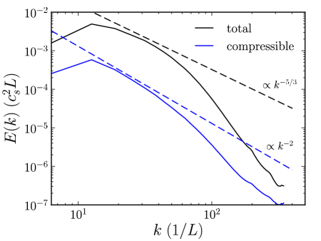
Figure 1.— 1D angle-averaged kinetic energy power spectra in our turbulence simulations. Simulating many “outer-scale” eddies in the parallel direction limits the inertial range of our turbulence to less than a decade.

Our analytical estimates in §2 are given in terms of arbitrary power spectra for the turbulent fluctuations. In many cases, the diffusion and acceleration of particles in the presence of pitch-angle scattering is dominated by interactions with a particular scale in the turbulence, typically either the smallest or largest scale in the inertial range. In this case, simulating a large inertial range may not be critical, though it would obviously be preferable. Later in the paper we highlight the specific results that we suspect may be most influenced by our limited dynamic range.

3.2. Test particle integration

Our particle integration methods are described in detail in Lehe et al. (2009). Particles are initialized in the fully saturated turbulence, and then evolved according to the Lorentz force. The $E$ and $B$-fields are those on the MHD grid, interpolated to the particle’s location using the triangular-shaped cloud (Hockney & Eastwood, 1981) method in space and time. Particles are integrated using the Boris (1970) particle pusher, which is sympletic and symmetric in time, and conserves energy and the magnetic moment adiabatic invariant to machine precision in tests with constant fields. We initialize particles randomly across the simulation domain with the initial values of $v_{\perp}$ and $v_{\parallel}$ defined relative to the local rest-frame of the MHD fluid in the simulation. More details are provided in Lehe et al. (2009).

3.2.1 Pitch-angle scattering

We implement pitch-angle scattering by specifying a scattering rate, $\nu$. We consider two cases to bracket the likely range of physical scattering mechanisms. The first is when the scatterers are at rest in the fluid frame. This seems likely to be appropriate for scattering by mirror or firehose instabilities, but not by, e.g., Alfvén waves, which move relative to the fluid frame at the Alfvén speed. We consider scatterers moving along the local magnetic field direction to model the latter.

At each scattering timestep $dt_{s}$ (defined below), and for each test particle, we subtract off the local fluid velocity, to perform the scattering in the fluid frame. For the simulations with moving scatterers, we move into the frame of the scatterer by subtracting off a further component of the velocity $\pm v_{s}\hat{b}$, where $\hat{b}$ is the local magnetic field direction and the scatterer is randomly chosen to be moving forward or backward in the fluid frame. We choose an isotropic random unit vector $\hat{e}_{1}$. We then calculate $\hat{e}_{2}=\hat{e}_{1}\times\hat{v}$, i.e., a unit vector perpendicular to the particle velocity $\mathbf{v}$. We rotate the test particle’s velocity vector around $\hat{e}_{2}$ through a random angle uniformly distributed between 0 and $\theta_{\mathrm{max}}$. $\hat{e}_{2}$ is chosen to be perpendicular to $\mathbf{v}$ so that the rotation of $\hat{v}$ occurs along a great circle on the unit sphere. We choose the timestep for the scattering procedure according to $dt_{s}=\theta_{\mathrm{max}}^{2}/(6\nu)$. We implement this rotation using Rodrigues’ rotation formula. Finally, the local fluid velocity (in addition to any scatterer velocity as appropriate) is added back to the particle’s velocity to return us to the lab frame.

This procedure ensures that the pitch-angle scattering rate is in fact given by our input parameter $\nu$ as long as $\theta_{\mathrm{max}}\ll 2\pi$, so that scattering is dominated by small changes in pitch-angle. We typically choose $\theta_{\mathrm{max}}=0.6$, which is sufficiently small that diffusion coefficients differ by less than 1% from their saturated values at $\theta_{\mathrm{max}}\rightarrow 0$, while minimizing computational effort associated with frequent scatterings.

In addition to diffusion in velocity space, pitch-angle scattering also leads to spatial diffusion with a mean free path $\lambda_{\parallel}\sim v/\nu$ and a diffusion coefficient $\kappa_{\parallel}=(2/3)v^{2}/\nu$, where the parallel subscript indicates that the spatial diffusion is still primarily along magnetic field lines in our calculations. In particular, perpendicular spatial diffusion $\kappa_{\perp}$ is $\sim r_{G}^{2}\nu$, where $r_{G}$ is the particle gyroradius. We simulate high-gyrofrequency particles with small $r_{G}$ and so perpendicular diffusion is negligible even at the highest $\nu$ we consider.

3.3. Calculating Velocity Diffusion Coefficients

The velocity diffusion coefficients are calculated according to the formal definition

$$D\equiv\frac{\langle\delta v^{2}\rangle}{2\,\delta t},$$ (11)

where the average is over many particles with the same initial velocity. However, one subtlety is that a particle which experiences no acceleration can nevertheless appear to change velocity when measured with respect to the local fluid frame. This is because the fluid’s parallel velocity can change even if a given test particle feels no electromagnetic acceleration. Thus, absent pitch-angle scattering, after a time of order the correlation time of the fluid, an ensemble of particles initially at rest relative to the fluid will develop a finite dispersion in parallel velocity given by $\delta v\sim v_{\parallel,\mathrm{rms}}$ of the turbulence. (This effect becomes less significant at high pitch-angle scattering rates because the particles are ‘pinned’ near the location in the fluid where they are initialized.) Figure 2 plots two representative $\langle\delta v^{2}\rangle(t)$ curves and shows a rapid increase in $\langle\delta v^{2}\rangle(t)$ at early times for the low scattering rate calculation. To not include this in our diffusion coefficient calculations, we measure diffusion coefficients by instead fitting a straight line after the initial jump using least-squares (as indicated in Fig. 2).

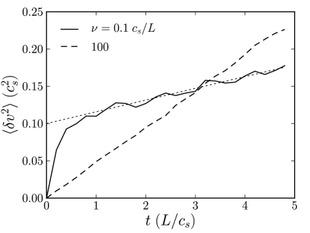
Figure 2.— Dispersion in velocity, measured relative to the fluid frame, as a function of time for test particles that were initially delta-functions with $v_{i}\simeq 0.025\,c_{s}$. The turbulence has properties given by Table 1. For the low-scattering run there is an initial “jump” in velocity dispersion caused by the changing local parallel fluid velocity relative to the particles, after which $\langle\delta v^{2}\rangle(t)$ increases linearly, consistent with diffusion. The high-scattering run has no such jump because the particles remain tied to the local fluid frame by the rapid scattering. The dotted curve shows the fit we use to calculate diffusion coefficients in the case with the initial jump.

4. Test-particle Diffusion and Heating

4.1. Velocity Diffusion: Stationary Scatterers

Figures 3 and 4 show diffusion coefficients for a broad range of pitch-angle scattering rates $\nu$ for our fiducial simulation (Table 1); the scattering is isotropic in the fluid frame. The chosen values of $\nu$ include scattering times significantly longer than, and significantly shorter than, the outer-scale turnover time of the turbulence. At the lowest scattering rates ($\nu\sim 10^{-3}-10^{-1}\,c_{s}/L$, corresponding to scattering times somewhat smaller than the nonlinear timescale of the turbulent fluctuations), the diffusion coefficient is well approximated by the pitch-angle average of the parallel diffusion coefficient appropriate for resonance broadened TTD + Fermi Type-B diffusion described in §2.1 (cyan line in Fig. 3). In this limit, scattering isotropizes the velocity-space diffusion but does not fundamentally alter the physics of how particles interact with the turbulent fluctuations.

For scattering rates $0.1\,c_{s}/L\lesssim\nu\lesssim 10\,c_{s}/L$, the diffusion coefficient increases at low velocity but not significantly for $v\gtrsim{\rm few}\,c_{s}$. The reason is that large-scale eddies produce the Fermi Type-B diffusion at low velocities – these interactions are thus fundamentally altered once the scattering rate is comparable to the frequency of the large-scale eddies. By contrast, eddies of all scales (including, in particular, small scales) contribute significantly to the high velocity TTD diffusion. The small scale eddies have higher nonlinear frequencies and thus a higher scattering rate is needed to modify the velocity-space diffusion of high speed particles.

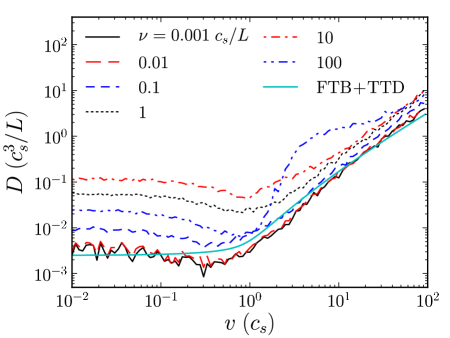
Figure 3.— Test particle velocity diffusion coefficients for low scattering rates for the fiducial simulation (see Table 1). Scatterers are stationary in the fluid frame. The solid cyan curve is a fit to a functional form given by a sum of Fermi Type-B and resonance-broadened transit-time damping in which particles interact with turbulent fluctuations in magnetic field strength. This provides a reasonable description at low scattering rates and/or high velocities. At high scattering rates ($\nu\sim 100c_{s}/L$), however, the functional form of the diffusion coefficient in the test particle calculations changes significantly. This corresponds to the transition to a non-resonant regime in which particles interact primarily with turbulent density fluctuation (see Fig. 4 and §2.2).

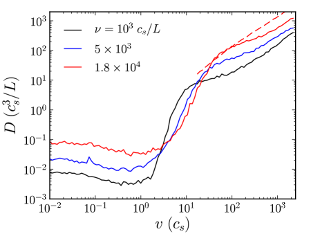
Figure 4.— Test particle velocity diffusion coefficients for the fiducial simulation at high scattering rates (solid curves), corresponding to the non-resonant regime discussed in §2.2. Scatterers are stationary in the fluid frame. For high velocities, the numerical results are reasonably well-approximated by eq. 9 (dashed curve), which describes velocity diffusion by non-resonant interactions with turbulent density fluctuations. The rapid increase in the diffusion coefficient with velocity at intermediate velocities $\sim{\rm few}\,c_{s}$ can produce a non-thermal tail in the distribution function (see Fig. 9).

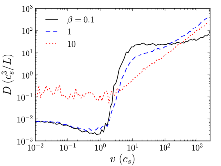
Figure 5.— Test particle velocity diffusion coefficients for $\nu=10^{3}c_{s}/L$ for three different $\beta$, corresponding to the non-resonant regime discussed in §2.2. Scatterers are stationary in the fluid frame. The results are similar for low $\beta\lesssim 1$ where slow modes dominate the compressional fluctuations. For $\beta=10$ the diffusion coefficient resembles the $\beta=1$ results at much lower scattering rates (see Fig. 3). This is because the compressional energy is significantly lower in the $\beta=10$ simulation, which decreases the efficiency of the non-resonant diffusion.

For $\nu\gtrsim 100\,c_{s}/L$, there is a qualitative change in the properties of the velocity diffusion coefficients in Figures 3 and 4, particularly for particles with $v\gtrsim c_{s}$. This corresponds to the onset of non-resonant diffusion governed by interactions between particles and turbulent density fluctuations. The properties of the high scattering rate diffusion depend on the ratio of the diffusion time to the wave period $\tau_{\mathrm{diff}}/\tau_{w}\propto\nu/v^{2}$. Lower velocity particles are in the regime where $\tau_{\rm diff}\gtrsim\tau_{w}$ and equation 7 predicts that the velocity diffusion coefficient is a strong function of velocity, with $D\propto v^{4}$. This is consistent with the numerical results in Figures 3 and 4 for high scattering rates and intermediate velocities $v\sim 2-10\,c_{s}$. Note that we do not numerically recover Chandran (2003)’s prediction that compressible slow mode turbulence at $\beta\lesssim 1$ should produce a $D\propto v^{2}$ scaling due to the contribution of eddies of different scale $l$ in equation 7. This may be because the finite dynamic range in our simulations means that we do not capture the full inertial range of the turbulence (this is exacerbated by our anisotropic box [see Table 1], which is required in order to avoid artifacts due to periodic boundary conditions along the mean field). In the limit that eddies of a single spatial scale dominate the velocity diffusion, equation 7 implies $D\propto v^{4}$, consistent with our numerical results.

For yet higher velocity particles, $\tau_{\rm diff}\lesssim\tau_{w}$ and equation 9 predicts $D\propto v$ in the rapid scattering limit. This is consistent with the numerical results in Figures 3 and 4. Quantitatively, the non-resonant regime of equation 9 requires simultaneously satisfying $l_{D}\gg\lambda_{\mathrm{mfp}}=v/\nu$ and $\tau_{\mathrm{diff}}\ll\tau_{w}$, which restricts us to the following range of velocities:

$$\nu l_{D}^{2}/\tau_{\mathrm{w}}\ll v^{2}\ll\nu^{2}l_{D}^{2}.$$ (12)

For the simulation with $\nu=5\times 10^{3}\,c_{s}/L$, the high-velocity non-resonant diffusion is appropriate in our test particle calculations for $73\ll v/c_{s}\ll 1950$, while for $\nu=1.8\times 10^{4}\,c_{s}/L$, particles with $140\ll v/c_{s}\ll 5700$ should satisfy equation 9. In Figure 4, we include the prediction of equation 9 for the $\nu=1.8\times 10^{4}\,c_{s}/L$ simulation as a dashed curve (measuring $\nabla\cdot u$ and $\tau_{\rm corr}$ as in §3.1.1 to determine the predicted normalization of $D$). The velocity diffusion is reasonably well approximated by equation 9 in the appropriate velocity interval.

Figure 5 shows how the diffusion coefficient in the high scattering rate, non-resonant regime depends on $\beta$ (for fixed $\nu=10^{3}c_{s}/L$). The turbulence has the same driving as in the fiducial simulation in Table 1. The key difference in the resulting turbulence properties is that the fraction of the turbulent energy in compressional fluctuations (those $\propto\nabla\cdot v$; see §3.1.1) is only $\sim 1.5\%$ for $\beta=10$ versus $10\%$ and $17\%$ for $\beta=1$ and $0.1$, respectively. This is because fast modes dominate the compressional fluctuations at high $\beta$ and are not efficiently excited in subsonic turbulence with solenoidal driving.

The results for the diffusion coefficient in Figure 5 are similar for $\beta=1$ and $\beta=0.1$. This is consistent with the fact that at low $\beta$ slow magnetosonic modes dominate the compressional fluctuations and are energetically important in MHD turbulence. By contrast, the diffusion coefficient changes significantly at $\beta\sim 10$, where fast modes dominate the compressional fluctuations. In particular, the $\beta=10$ results with $\nu=10^{3}\,c_{s}/L$ in Figure 5 are similar to the $\beta=1$ results at a much lower $\nu\sim 10\,c_{s}/L$ (see Fig. 3). This is because of the much lower compressional energy in the $\beta=10$ simulation, which decreases the efficiency of the non-resonant diffusion (see §2.2).

4.2. Velocity Diffusion: Moving Scatterers

Figure 6 shows test particle results from simulations with moving scatterers. The velocity diffusion coefficient is nearly independent of particle velocity. These results are consistent with Fermi-like scattering predicted by equation 10, namely $D\sim v_{s}^{2}\nu$. At sufficiently high velocity, the non-resonant diffusion $D\propto v$ shown in Figures 3 and 4 would eventually dominate over the roughly constant diffusion coefficient shown in Figure 6.

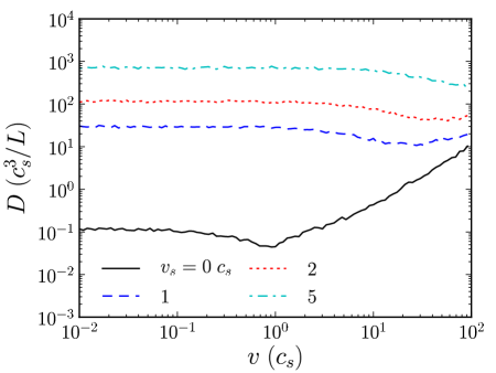
Figure 6.— Test particle velocity diffusion coefficients for the fiducial simulation with $\nu=10\,c_{s}/L$ and scatterers moving at various velocities $v_{s}$. The moving scatterers cause Fermi-like velocity diffusion consistent with $D\sim v_{s}^{2}\nu$ (see eq. 10 and §2.2.1).

4.3. Test-particle heating

Figure 7 shows how the pitch-angle scattering rate $\nu$ affects the heating of test particles that have an initially Maxwellian distribution with thermal speed $v_{\rm th}$. The $\nu=10^{-3}c_{s}/L$ results shown are nearly identical to the heating rates in the absence of pitch-angle scattering. For the calculations in Figure 7, we assume that the scattering is at rest in the local fluid frame. Note that for our fiducial simulation parameters (Table 1), protons correspond to $v_{\rm th}=c_{s}/\sqrt{2}$, electrons to $v_{\rm th}\simeq 30c_{s}$ and minor ions (with temperatures of order the proton temperature) to $v_{\rm th}\lesssim c_{s}$ in Figure 7.

Not surprisingly, the enhanced velocity diffusion shown in Figures 3 and 4 leads to a corresponding increase in the net particle heating rate. At the scattering rates we focus on here, this increase in the heating rate is a consequence of pitch-angle scattering enforcing isotropy, which leads to a substantially enhanced TTD heating rate at $v\gtrsim c_{s}$ and an enhanced FTB heating rate at low velocities. Quantitatively, Figure 7 shows that even a modest scattering rate, with $\nu^{-1}$ comparable to the outer-scale turbulent correlation time ($\sim 0.1L/c_{s}$; see Table 1), can increase the net heating rate significantly so that a large fraction of the compressible turbulent energy can go into heating protons. Moreover, when $\dot{\epsilon}_{\rm test}\gtrsim\dot{\epsilon}$ for protons, our test particle assumption breaks down because the protons will absorb the majority of the compressible turbulent power on large scales in the turbulent cascade. Figure 7 also shows that minor ion heating is particularly effective if the ions and protons have comparable temperatures, so that the minor ions have lower thermal velocities. This is true, e.g., in the slow speed solar wind but not in the fast solar wind, where the ion and proton thermal velocities are comparable (Bochsler, 2007); in this case, our results imply comparable proton and minor ion heating rates per particle.

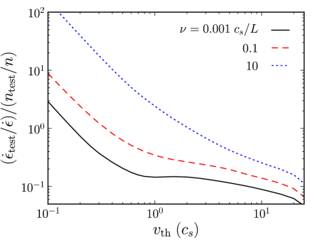
Figure 7.— Particle heating rate $\dot{\epsilon}_{\rm test}$, normalized by the turbulent cascade rate $\dot{\epsilon}$, as a function of thermal velocity $v_{\rm th}$, for an initially Maxwellian distribution function. The heating rate is measured from $t=2.5-20L/c_{s}$ in the fiducial simulation and is $\propto n_{\rm test}/n$, where $n_{\rm test}/n$ is the number density of test particles relative to the fluid density in the simulation. Modest pitch-angle scattering rates $\nu$ enforce isotropy and significantly enhance the turbulent heating of the plasma.

5. Power-law tails?

Figure 8 shows the late-time distribution function that results when we evolve test particles which initially have a Maxwellian with $v_{\rm th}=c_{s}$ in our fiducial turbulence simulation (Table 1), for several different scattering rates. The evolution is for $\sim 20\,L/c_{s}$, which is many eddy turnover times. These results are very similar to the analogous results without pitch-angle scattering in our earlier work (Lynn et al., 2012). In particular, Figure 8 demonstrates that at low to moderate scattering rates the particles are efficiently heated by the turbulence (more-so with increasing $\nu$; see Fig. 7), but no significant non-thermal power-law tail develops. Recall that this scattering rate regime corresponds to the particles gaining energy from turbulent magnetic compressions (as in linear TTD of fast and slow magnetosonic waves).

Figure 9 shows the evolution of the distribution function for $\nu=10^{3}\,c_{s}/L$ for two initial thermal velocities, $v_{\rm th}=0.5$ and $2\,c_{s}$ (these two different thermal velocities are included to highlight the physics of the distribution function evolution at high $\nu$; below we also summarize results for calculations with $v_{\rm th}=c_{s}$, more relevant for protons). In the high scattering rate calculations in Figure 9, the resulting distribution function is qualitatively different: there is a nearly power-law component over almost a decade in velocity, particularly for $v_{\rm th}=2\,c_{s}$. The non-thermal tail also becomes more energetically important at later times, after the distribution function has been evolved for $\sim 20L/c_{s}$. There is no evidence for a universal power-law slope in the velocity distribution function in this regime of rapid pitch-angle scattering. Instead, the exact slope depends sensitively on time, the pitch-angle scattering rate, and the thermal velocity of the test particle distribution: for $v_{\rm th}=2\,c_{s}$, $f\propto v^{-3.5}$ at $t=5L/c_{s}$ and $f\propto v^{-1.5}$ at $t=20L/c_{s}$ while for $v_{\rm th}=0.5\,c_{s}$, $f\propto v^{-7.5}$ at late times and is not convincingly a power-law at earlier times.

The significant non-thermal tail to the distribution function in Figure 9 is caused by the steep scaling of the velocity diffusion coefficient with $v$ for intermediate velocities seen in Figure 4. The ‘strength’ of this power-law tail depends, however, on the assumed pitch-angle scattering rate and the thermal speed of the test particles since this determines how well the $D\propto v^{4}$ diffusion coefficient regime in Figure 4 overlaps with the initial Maxwellian of the test particles. Higher scattering rates lead to $D\propto v^{4}$ setting in at higher velocity. This implies significantly less efficient acceleration of particles out of the thermal population. Thus a strong power-law tail requires fine-tuning between the scattering rate and the thermal velocity of the species of interest. Quantitatively, the power-law tail in Figure 9 is much less significant for $v_{\rm th}=0.5c_{s}$ relative to $v_{\rm th}=2c_{s}$. In addition, in calculations with $v_{\rm th}=1\,c_{s}$ (more appropriate for protons), which are not explicitly shown here, we find that after $\simeq 5\,L/c_{s}$ interacting with our fiducial turbulence (Table 1), the distribution function roughly satisfies $f(v)\propto v^{-3.5}$ for $\nu\simeq 100\,c_{s}/L$, $f(v)\propto v^{-6.5}$ for $\nu\simeq 10^{3}\,c_{s}/L$, and $f(v)\propto v^{-10}$ for $\nu\simeq 10^{4}\,c_{s}/L$ over the velocity range $v\sim 3-10\,c_{s}$. This highlights the strong dependence of the resulting distribution function on all of the parameters of the problem.

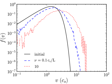
Figure 8.— An initially Maxwellian distribution of test particles with thermal velocity $v_{\rm th}=c_{s}$ is simulated for $t=20L/c_{s}$ (many eddy turnover times) in our fiducial simulation (Table 1), with two different values of the imposed scattering rate $\nu$. The final distribution functions are slightly non-Maxwellian but do not develop a significantly non-thermal tail. $f(v)$ shown here is the one-dimensional distribution function, normalized such that the density is $n_{0}=\int dvf(v)$.

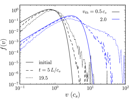
Figure 9.— Initially Maxwellian distributions of test particles with $v_{\rm th}=0.5$ and $2\,c_{s}$ are simulated for $t=20L/c_{s}$ (many eddy turnover times), with a high scattering rate $\nu=10^{3}\,c_{s}/L$. We show the initial (solid) and final (dotted) distributions, as well as at an intermediate time (dashed). Power-law tails develop in the velocity regime with the enhanced $D\propto v^{4}$ velocity diffusion in Fig. 4. There is not, however, a ‘universal’ power-law slope to the resulting distribution function. Instead, the slope depends on time, thermal velocity of the distribution, and pitch-angle scattering rate (the latter dependence is not explicitly shown here). $f(v)$ shown here is the one-dimensional distribution function, normalized such that the density is $n_{0}=\int dvf(v)$.

The absence of a non-thermal tail at low scattering rates in Figure 8 is consistent with the general form of the diffusion coefficient in Figure 3, in particular the fact that the diffusion coefficient scales at most $\propto v\log[v]$. Green’s function solutions of the diffusion equation show that only if the diffusion coefficient scales as $D\propto v^{2}$ or steeper does velocity diffusion alone generically produce a strong non-thermal tail to the distribution function (e.g., Gruzinov & Quataert 1999; Jokipii & Lee 2010). This is consistent with our numerical results in Figure 8.

In his original analysis, Fermi invoked a competition between velocity diffusion and particle escape in order to obtain a power-law distribution function. Our simulations do not explicitly have escape and one might thus worry that the absence of a power-law tail is an artifact of the periodic boundary conditions in our calculations. This is not the case.

In the presence of particle escape, the combination of diffusion and escape produces a power-law tail only if the ratio of the acceleration time $\tau_{a}\equiv v^{2}/D$ to the escape time $\equiv\tau_{e}$ is independent of particle energy (e.g. Longair, 1992). In our problem, a well-posed question is whether escape due to spatial diffusion, which is self-consistently produced by pitch-angle scattering, produces the requisite conditions for a power-law tail. Scattering implies $\kappa\sim v^{2}/\nu$ so that $\tau_{e}\propto\nu/v^{2}$. If $\nu$ is roughly independent of velocity, only a very steep diffusion coefficient of the form $D\propto v^{4}$ can produce a power-law tail in the presence of diffusive escape. This is the regime in which we already find a significant non-thermal tail in Figure 9. The velocity diffusion coefficient that results from most of our calculations is (roughly) $D\propto v$, i.e., $\tau_{a}\propto v$. This applies in both the quasi-resonant limit and in the high scattering rate limit at high velocities. Thus, unless for some reason $\nu\propto v^{3}$, so that $\tau_{e}\propto v$, weakly compressible MHD turbulence will not generically produce a significant non-thermal tail in the $D\propto v$ regime even in the presence of particle escape.

6. Conclusions

We have studied the heating and acceleration of particles by subsonic MHD turbulence by evolving an ensemble of test particles in real time in MHD turbulence simulations. Our focus in this paper has been on the role of pitch-angle scattering in modifying the efficiency of non-relativistic particle heating and acceleration. To study this we have implemented explicit pitch-angle scattering (at a fixed rate $\nu$), with the scatterers either at rest in the fluid frame or moving relative to the fluid frame along the local magnetic field. We suspect that these two cases bracket reality in problems of interest, representing the role of mirror/firehose instabilities (which are non-propagating instabilities and thus roughly at rest in the fluid frame) and high frequency ion cyclotron, Alfvén, or whistler waves, respectively. In our calculations the scattering rate is independent of velocity, but this may not be the case in real systems. In particular, the mechanisms that dominate pitch-angle scattering may differ for thermal and super-thermal particles. Results for a velocity-dependent scattering rate can be obtained from the calculations presented here by appropriately interpolating between the diffusion coefficients for different scattering rates shown in Figures 3-5 (this is formally valid for our test particle calculations).

In all of our calculations, we have focused on the evolution of particles with gyrofrequencies much larger than the resolved frequencies of the turbulent fluctuations. In the absence of pitch-angle scattering, the magnetic moment of our test particles is thus conserved: particles only undergo diffusion in $v_{\parallel}$. The reason for restricting our analysis to these high gyrofrequency particles is that the outer scale turbulent fluctuations in astrophysical and heliospheric systems have frequencies much smaller than the particle gyrofrequencies. Thus the high gyrofrequency limit is the correct limit for studying particle heating and acceleration using MHD simulations. In addition, much of the energy in MHD turbulence cascades anisotropically in wave-vector space, and there is little power at frequencies comparable to the ion cyclotron frequency, even when the turbulent fluctuations have wavelengths comparable to the ion Larmor radii (e.g., Schekochihin et al. 2009). A corollary of this is that it is difficult to predict a priori what the pitch-angle scattering rate should be in a given astrophysical or heliospheric context, since it depends on kinetic processes that excite very high frequency fluctuations (relative to the MHD-scale turbulence that is better understood). We return to this point below when discussing the implications of our results for the solar wind.

We find that the physics of particle energization by MHD turbulence depends on the ratio of the mean free path set by pitch-angle scattering ($\lambda_{\rm mfp}\simeq v/\nu$) to the scale of the turbulent fluctuations $L$. For low scattering rates, i.e., $\lambda_{\rm mfp}\gtrsim L$, the particle energization is analogous to that in the collisionless limit and occurs primarily through quasi-resonant interactions with turbulent fluctuations in the local strength of the magnetic field. In linear theory, these field compressions would be associated with slow ($\beta\gg 1$) or fast ($\beta\ll 1$) magnetosonic modes and the resulting wave-particle interaction is often called transit-time damping (TTD). Pitch angle scattering increases the efficiency of this quasi-resonant heating mechanism by reducing the parallel acceleration of particles out of resonance and converting $v_{\parallel}$ heating into $v_{\perp}$ heating, thus increasing the magnitude of the $\mu\nabla B$ force associated with magnetic field compressions (Achterberg, 1981). The net heating rate for thermal particles can be a factor of $\sim 3-10$ larger in the presence of modest pitch-angle scattering ($\nu\sim c_{s}/L$; Fig. 7).

In the limit of rapid pitch-angle scattering, the physical process leading to particle energization is fundamentally different. Our numerical results in this limit are consistent with the analytic calculations of Ptuskin (1988) and Chandran & Maron (2004). Physically, at high scattering rates, particles are nearly pinned to the frame of the scatterers. To first approximation, particles thus adiabatically heat and cool as they move through density fluctuations in the plasma. Spatial diffusion of particles relative to the density fluctuations ultimately makes this energy change diffusive rather than reversible. Note that the energy source for particle energization in the rapid scattering limit is turbulent density compressions and rarefactions, rather than the turbulent magnetic field compressions that are important at low scattering rates. In linear theory, these density fluctuations are associated with fast modes at $\beta\gg 1$ and both slow and fast modes at $\beta\ll 1$. In addition to coupling to the turbulent density compressions, if the scatterers are moving relative to the fluid frame, pitch-angle scattering produces a Fermi-like velocity kick that corresponds to a velocity diffusion coefficient that is independent of velocity for non-relativistic particles (eq. 10 and Fig. 6).

One of our primary motivations for including the effects of pitch-angle scattering was to assess whether pitch-angle scattering increases the efficiency of particle acceleration by MHD turbulence, i.e., the generation of a non-thermal tail in the distribution function. We find that this is not the case at low scattering rates where quasi-resonant interactions with magnetic field compressions dominate the velocity diffusion (see Fig. 8). Although particle heating is quite effective, with heating rates for thermal protons comparable to the energy cascade rate in the turbulence, the distribution function does not develop a significant non-thermal tail. This conclusion from our test particle simulations is consistent with solutions of the Fokker-Planck equation given the velocity diffusion coefficient we find at low scattering rates, namely $D\propto v$ for $v\gtrsim c_{s}$ (Fig. 3).

For high scattering rates, $\nu\sim 10^{2-4}c_{s}/L$, we find that the distribution function can develop a non-thermal tail, but only under certain relatively restrictive conditions. The power-law tail arises due to the strong scaling $D\propto v^{4}$ that occurs at intermediate velocities $\sim{\rm few}\,c_{s}$ in the rapid scattering limit (eq. 7 and Fig. 4). At high particle velocities, the diffusion coefficient varies much more weakly with velocity ($D\propto v$) and so does not produce efficient acceleration. Physically, the transition between $D\propto v^{4}$ and $D\propto v$ occurs when the spatial diffusion time ($\propto\nu/v^{2}$) across an eddy becomes shorter than the eddy turnover time, as predicted in Ptuskin (1988)’s original analysis. This produces a significant power-law tail only if the transition between the two diffusion regimes occurs at a velocity comparable to the thermal velocity of the particles of interest (Fig. 9). This requires fine tuning between the pitch-angle scattering rate and the thermal velocity of the particles.

What are the implications of our results for particle heating and acceleration in the solar wind, the most well-studied and well-constrained astrophysical plasma to which our results can be applied? This depends to some extent on the effective scattering rate in the low-collisionality solar wind. Given the ubiquitous in situ evidence for significant temperature anisotropies in the thermal plasma in the solar wind (e.g., Kasper et al. 2002) it is likely that the effective scattering rate for the thermal plasma cannot be much larger than the expansion rate of the solar wind $\sim R/v_{\rm wind}$ (where $R$ is the local radius, i.e., $\sim 1$ AU near Earth). On the other hand, the measured temperature anisotropies in the solar wind also appear to be constrained by the thresholds for mirror, firehose, and (to a lesser extent) ion cyclotron instabilities, suggesting that there is some minimum level of pitch-angle scattering even in nearly collisionless epochs. Expansion of the solar wind inevitably drives solar wind plasma towards these instability thresholds (e.g., Hellinger & Trávníček 2008). Together, these arguments suggest that the effective scattering rate for thermal plasma is $\nu\sim v_{\rm wind}/R$, which is in turn $\sim c_{s}/L$ where $L\sim 0.03R$ is the outer-scale of turbulence in the near-Earth solar wind (e.g., Howes et al. 2008) and $v_{\rm wind}\sim 10c_{s}$. Measurements of anisotropies in the distribution function at $v\sim 10c_{s}$ (at distances of a few AU) suggest that the mean free path is of order an AU (Gloeckler et al., 1995), implying a comparable effective scattering rate for super-thermal particles. These estimates are probably only accurate to a factor of $10$, but this is sufficient to draw several important conclusions.

First, pitch-angle scattering likely enhances heating of the thermal particles by the compressible part of the cascade (which is primarily slow modes in the near-Earth solar wind; Yao et al. 2011; Howes et al. 2012) by factors of a few-10 (Fig. 7). Secondly, Figure 8 shows that even in the presence of pitch-angle scattering with $\nu\sim c_{s}/L$, the particle distribution function does not develop a significant non-thermal tail due to MHD-scale turbulent fluctuations. Moreover, even if we optimistically assume that $\nu\gtrsim 100\,c_{s}/L$ (in spite of the evidence for anisotropic distribution functions in the solar wind), our results do not imply that rapid pitch-angle scattering would produce a power-law tail in the proton distribution function in the near-Earth solar wind. The reason is that the particle acceleration time implied by Figure 4 ($t_{\rm a}\simeq v^{2}/D$) is longer than the expansion time of the solar wind $R/v_{\rm wind}\sim L/c_{s}$ over the entire velocity regime in which $D\propto v^{4}$. This is even more true when we take into account that the compressional energy in the solar wind – which is the important energy source in the presence of pitch-angle scattering – is somewhat smaller than in our simulations: e.g., $\delta n/n\simeq 0.1$ in the solar wind vs. $\delta n/n\simeq 0.23$ in our fiducial $\beta=1$ simulation (see §3.1.1). Thus in the context of the near-Earth solar wind, adiabatic cooling (not present in our calculations) dominates particle acceleration by MHD turbulence even for very rapid pitch-angle scattering; this would preclude the power-law tail seen in Figure 9 from developing.

Taken together, these considerations strongly argue against the MHD scale fluctuations as the source of the $v^{-5}$ tail in the proton distribution function observed throughout the heliosphere (Gloeckler, 2003; Fisk & Gloeckler, 2006). It does not, of course, preclude that kinetic-scale physics acting on small scales in the turbulent cascade could produce such a non-thermal tail (e.g., via reconnection or kinetic Alfvén wave turbulence). In addition, our conclusions are based primarily on the well-studied plasma conditions near $\sim 1$ AU. If the pitch-angle scattering rate and/or the compressibility of the turbulence are significantly larger at larger radii in the solar wind, the compressible part of the turbulence may be important for producing a significant non-thermal tail.

Although we have focused the discussion of our results on the solar wind application because of the wealth of in situ measurements, the calculations presented here are much more broadly applicable. For example, particle heating and acceleration by MHD turbulence has been widely used to model solar flares and the “re-acceleration” of cosmic rays in the Milky Way and clusters of galaxies. Some of these applications would require generalizing our techniques to relativistic particles, but this is straightforward.

References

- Achterberg (1981) Achterberg, A. 1981, Astronomy & Astrophysics, 97, 259
- Bale et al. (2009) Bale, S., Kasper, J., Howes, G., Quataert, E., Salem, C., & Sundkvist, D. 2009, Physical Review Letters, 103, 211101
- Bellamy et al. (2005) Bellamy, B. R., Cairns, I. H., & Smith, C. W. 2005, Journal of Geophysical Research (Space Physics), 110, 10104
- Bieber et al. (1994) Bieber, J. W., Matthaeus, W. H., Smith, C. W., Wanner, W., Kallenrode, M.-B., & Wibberenz, G. 1994, The Astrophysical Journal, 420, 294
- Bochsler (2007) Bochsler, P. 2007, A&A Rev., 14, 1
- Boris (1970) Boris, J. 1970, in Proceedings of the Fourth Conference on Numerical Simulations of Plasmas, Naval Research Lab, 3–67
- Breech et al. (2009) Breech, B., Matthaeus, W. H., Cranmer, S. R., Kasper, J. C., & Oughton, S. 2009, Journal of Geophysical Research (Space Physics), 114, 9103
- Chandran (2003) Chandran, B. D. G. 2003, The Astrophysical Journal, 599, 1426
- Chandran et al. (2010) Chandran, B. D. G., Li, B., Rogers, B., Quataert, E., & Germaschewski, K. 2010, The Astrophysical Journal, 720, 503
- Chandran & Maron (2004) Chandran, B. D. G., & Maron, J. L. 2004, The Astrophysical Journal, 603, 23
- Cho & Lazarian (2003) Cho, J., & Lazarian, A. 2003, Monthly Notices of the Royal Astronomical Society, 345, 325
- Fermi (1949) Fermi, E. 1949, Physical Review, 75, 1169
- Fisk & Gloeckler (2006) Fisk, L., & Gloeckler, G. 2006, The Astrophysical Journal Letters, 640, 79
- Fisk & Gloeckler (2008) —. 2008, The Astrophysical Journal, 686, 1466
- Giacalone & Jokipii (1994) Giacalone, J., & Jokipii, J. R. 1994, The Astrophysical Journal, 430, L137
- Gloeckler (2003) Gloeckler, G. 2003, AIP Conference Proceedings, 679, 583
- Gloeckler et al. (1995) Gloeckler, G., Schwadron, N. A., Fisk, L. A., & Geiss, J. 1995, Geophys. Res. Lett., 22, 2665
- Goldreich & Sridhar (1995) Goldreich, P., & Sridhar, S. 1995, The Astrophysical Journal, 438, 763
- Gruzinov & Quataert (1999) Gruzinov, A., & Quataert, E. 1999, The Astrophysical Journal, 520, 849
- Hellinger & Trávníček (2008) Hellinger, P., & Trávníček, P. M. 2008, Journal of Geophysical Research, 113, A10109
- Hockney & Eastwood (1981) Hockney, R., & Eastwood, J. 1981, Computer Simulation Using Particles (CRC Press)
- Howes et al. (2012) Howes, G. G., Bale, S. D., Klein, K. G., Chen, C. H. K., Salem, C. S., & TenBarge, J. M. 2012, The Astrophysical Journal, 753, L19
- Howes et al. (2008) Howes, G. G., Cowley, S. C., Dorland, W., Hammett, G. W., Quataert, E., & Schekochihin, A. A. 2008, Journal of Geophysical Research, 113, 1
- Jokipii (1966) Jokipii, J. R. 1966, The Astrophysical Journal, 146, 480
- Jokipii & Lee (2010) Jokipii, J. R., & Lee, M. A. 2010, The Astrophysical Journal, 713, 475
- Kasper et al. (2002) Kasper, J. C., Lazarus, A. J., & Gary, S. P. 2002, Geophysical Research Letters, 29, 1839
- Kennel & Engelmann (1966) Kennel, C., & Engelmann, F. 1966, Physics of Fluids, 9, 2377
- Kowal & Lazarian (2010) Kowal, G., & Lazarian, a. 2010, The Astrophysical Journal, 720, 742
- Lehe et al. (2009) Lehe, R., Parrish, I. J., & Quataert, E. 2009, The Astrophysical Journal, 707, 404
- Longair (1992) Longair, M. S. 1992, High Energy Astrophysics, 2nd edn. (Cambridge University Press)
- Lynn et al. (2012) Lynn, J. W., Parrish, I. J., Quataert, E., & Chandran, B. D. G. 2012, The Astrophysical Journal, 758, 78
- Mace et al. (2000) Mace, R. L., Matthaeus, W. H., & Bieber, J. W. 2000, The Astrophysical Journal, 538, 192
- Maechler et al. (2012) Maechler, M., et al. 2012, sfsmisc: Utilities from Seminar fuer Statistik ETH Zurich, R Package Version 1.0-20
- Ng et al. (2010) Ng, C. S., Bhattacharjee, A., Munsi, D., Isenberg, P. A., & Smith, C. W. 2010, Journal of Geophysical Research (Space Physics), 115, 2101
- Ptuskin (1988) Ptuskin, V. 1988, Soviet Astronomy Letters, 14, 255
- Qin & Shalchi (2012) Qin, G., & Shalchi, A. 2012, Advances in Space Research, 49, 1643
- R Core Team (2012) R Core Team. 2012, R: A Language and Environment for Statistical Computing, R Foundation for Statistical Computing, Vienna, Austria, ISBN 3-900051-07-0
- Schekochihin et al. (2008) Schekochihin, A., Cowley, S., Kulsrud, R., Rosin, M., & Heinemann, T. 2008, Physical Review Letters, 100, 081301
- Schekochihin et al. (2009) Schekochihin, A. A., Cowley, S. C., Dorland, W., Hammett, G. W., Howes, G. G., Quataert, E., & Tatsuno, T. 2009, The Astrophysical Journal Supplement Series, 182, 310
- Shalchi et al. (2004) Shalchi, A., Bieber, J. W., Matthaeus, W. H., & Qin, G. 2004, The Astrophysical Journal, 616, 617
- Sharma et al. (2007) Sharma, P., Quataert, E., Hammett, G. W., & Stone, J. M. 2007, The Astrophysical Journal, 667, 714
- Skilling (1971) Skilling, J. 1971, The Astrophysical Journal, 170, 265
- Skilling (1975) —. 1975, Monthly Notices of the Royal Astronomical Society
- Stone et al. (2008) Stone, J., Gardiner, T. A., Teuben, P., Hawley, J. F., & Simon, J. B. 2008, The Astrophysical Journal Supplement Series, 178, 137
- Tautz et al. (2013) Tautz, R. C., Lerche, I., & Kruse, F. 2013, Astronomy & Astrophysics, 555, A101
- Tu & Marsch (1995) Tu, C.-Y., & Marsch, E. 1995, Space Sci. Rev., 73, 1
- Yan & Lazarian (2008) Yan, H., & Lazarian, A. 2008, The Astrophysical Journal, 673, 942
- Yao et al. (2011) Yao, S., He, J.-S., Marsch, E., Tu, C.-Y., Pedersen, A., Rème, H., & Trotignon, J. G. 2011, ApJ, 728, 146