Streams in the Aquarius stellar haloes

Abstract

We use the very high resolution, fully cosmological simulations from the Aquarius project, coupled to a semi-analytical model of galaxy formation, to study the phase-space distribution of halo stars in “solar neighbourhood”-like volumes. We find that this distribution is very rich in substructure in the form of stellar streams for all five stellar haloes we have analysed. These streams can be easily identified in velocity space, as well as in spaces of pseudo-conserved quantities such as $E$ vs. $L_{z}$. In our best-resolved local volumes, the number of identified streams ranges from $\approx 300$ to 600, in very good agreement with previous analytical predictions, even in the presence of chaotic mixing. The fraction of particles linked to (massive) stellar streams in these volumes can be as large as $84\%$. The number of identified streams is found to decrease as a power-law with galactocentric radius. We show that the strongest limitation to the quantification of substructure in our poorest-resolved local volumes is particle resolution rather than strong diffusion due to chaotic mixing.

1 Introduction

In the last decade the characterization of the phase-space distribution of stars in the vicinity of the Sun has become a subject of great interest. It is now well-established that by studying the phase-space distribution function of the Milky Way we may be able to unveil its formation history (Freeman & Bland-Hawthorn, 2002; Helmi, 2008).

According to the current paradigm of galaxy formation, the stellar haloes of large galaxies such as our own are mostly formed through the accretion and mergers of smaller objects (Searle & Zinn, 1978), rather than by a rapid collapse of a large and pristine gas cloud (Eggen et al., 1962). During the process of accretion, these systems are tidally disrupted and contribute gas and stars to the final object. Whereas the gas component rapidly forgets its dynamical origin due to its dissipative nature, stars should retain this information for much longer time scales because their density in phase-space is conserved. This memory is especially easily accessible in the outer regions of galaxies, or outer stellar haloes, where the dynamical mixing time scales are very long. A large amount of observed stellar streams in the outer regions of the Milky Way supports this picture for the formation of its stellar halo. The Sagittarius stream (Ibata et al., 1994, 2001) and the Orphan stream (Belokurov et al., 2007) are just two examples among many other overdensities recently discovered (see also Newberg et al., 2002; Ibata et al., 2003; Yanny et al., 2003; Belokurov et al., 2006; Grillmair, 2006; Starkenburg et al., 2009).

This formation model also predicts that for Milky Way-like galaxies, the portion of the accreted stellar halo that dominates in the solar neighbourhood is dynamically old. (e.g. Cooper et al., 2010; Tissera et al., 2012). Therefore, fossil signatures of the most ancient accretion events that a galaxy has experienced should be buried in their inner regions or, in the case of the Milky Way, close to or in the Solar Neighbourhood. However, due to the very short dynamical time scales characteristic of these regions, debris from accretion events is expected to be spatially well-mixed and therefore rather difficult to detect. Furthermore, in cold dark matter models, dark matter haloes are expected to be strongly triaxial (see e.g. Allgood et al., 2006; Vera-Ciro et al., 2011). As a consequence, chaotic orbits may be quite important and result in much shorter mixing time-scales (see, e.g., Vogelsberger et al., 2008), which leads to a phase-space distribution that is effectively smooth. On the other hand, the dissipative condensation of baryons can induce a transformation of the structure of dark haloes to a more oblate and axisymmetric shape in the inner regions while preserving their triaxial shape in the outer parts (Debattista et al., 2008; Abadi et al., 2010; Valluri et al., 2010; Bryan et al., 2012).

The first attempt to quantify the amount of substructure in the form of stellar streams expected in the Solar Neighbourhood was carried out by Helmi & White (1999). They suggested that $\sim 300$ - $500$ kinematically-coherent substructures should be present in a local volume around the Sun. Although they considered a fixed Galactic potential, their results were later confirmed by Helmi et al. (2003), who analysed a full cosmological simulation of the formation of a cluster dark matter halo scaled down to galaxy size. They also showed that debris from accretion events appeared to mix on time-scales comparable to those expected for integrable potentials. However, their results were based on a single N-body simulation and were limited by its numerical resolution (despite the 66 million particles used).

Stellar streams in the inner regions of the Galactic halo cannot be detected simply by looking for overdensities in the distribution of stars on the sky. Thus, several different spaces have been proposed and explored to identify substructure. Examples are the velocity space (Helmi & White, 1999; Helmi et al., 1999; Williams et al., 2011), metallicity, colour and chemical abundance spaces (e.g. Font et al., 2006; Schlaufman et al., 2011; Monachesi et al., 2013; Valluri et al., 2013) or spaces defined by integrals of motion and their associated orbital frequencies (e.g. Helmi & de Zeeuw, 2000; Bullock & Johnston, 2005; Knebe et al., 2005; McMillan & Binney, 2008; Klement et al., 2009; Morrison et al., 2009; Gómez & Helmi, 2010; Gómez et al., 2010). At first sight, these studies as well as that by Helmi et al. (2003) might be in tension with the results reported by Valluri et al. (2013). These authors found no substructure in the integral of motion space of halo stars formed in a fully cosmological hydrodynamical simulation. They attributed the lack of substructure to the strong chaotic mixing present in this simulation. Their results were based on samples of $\approx 10^{4}$ stellar particles distributed across the entire halo. This likely imposes a strong limitation on the ability to identify and quantify substructure. If, as discussed by Helmi et al. (2003), there are 300-500 streams crossing the Solar neighbourhood a resolution of at least a few thousand stars in a local small volume (of a few kpc across) is required. Hence a much larger number across the whole halo. Therefore samples of a total of 10,000 halo stars would really be too small to find or characterize substructure. We confirm this intuition below, where we show that substructure is clearly visible when the numerical resolution (particle number) is large enough.

Thanks to current surveys such as RAVE (Steinmetz et al., 2006) and SEGUE (Yanny et al., 2009), as well as the forthcoming astrometric satellite Gaia (Perryman et al., 2001), model predictions are becoming testable. Although to date only a handful of stellar streams have been detected in the Solar Neighbourhood (e.g. Helmi et al., 1999; Klement et al., 2009; Smith et al., 2009), with the full 6-D phase-space catalogues that are already becoming available (Breddels et al., 2010; Bond et al., 2010; Carollo et al., 2010; Zwitter et al., 2010; Burnett et al., 2011; Beers et al., 2012) it may soon be possible to start deciphering the formation history of the Milky Way.

In this work we revise the predictions made by Helmi et al. (2003). Our goal is to characterize and quantify the amount of substructure inside solar neighbourhood like volumes obtained from the fully cosmological very high resolution simulation of galactic stellar haloes modelled by Cooper et al. (2010). In Section 2 we briefly describe these models. We characterize the phase-space distribution of stellar particles in “solar neighbourhood” spheres in Section 3. In Section 4 we measure the number of stellar streams, and explore the relevance of orbital chaos for halo stars near the Sun, as well as the impact of particle resolution on the quantification of substructure. Finally, in Section 5 we summarise our results.

Throughout this work we use the term substructure only to refer to substructure in the form of stellar streams.

Table 1: Properties of the five Aquarius haloes used in this work at $z=0$. The first column labels the simulation. From left to right, the columns give the virial radius of the dark matter halo, $r_{200}$, the number of particles within $r_{200}$, the maximum circular velocity, $V_{\rm max}$, the particle mass, $m_{\rm p}$, the concentration parameter, $c_{\rm NFW}$, the intermediate to major, $b/a^{\it sn}$, and the minor to major, $c/a^{\it sn}$, axial ratios computed using dark matter particles located within 6 to 12 kpc, the total stellar halo mass, $M_{*}$, the corresponding half-light radius, $r_{1/2}$, the total stellar mass of the central galaxy in GALFORM, and the RMS scatter in the logarithm of the stellar mass assigned to the individual particles.

Name	$r_{200}$	$N_{200}$	$V_{\rm max}$	$m_{\rm p}$	$c_{{\rm NFW}}$	$b/a^{\it sn}$	$c/a^{\it sn}$	$M_{*}$	$r_{1/2}$	$M_{\rm gal}$	$\log_{10}~{}(m_{*})$
		[$10^{6}$]		[$10^{3}$]				[$10^{8}$]		[$10^{10}$]	RMS
A-2	$246$	$135$	$209$	$13.7$	$16.2$	$0.65$	$0.53$	$3.8$	$20$	$1.88$	$1.06$
B-2	$188$	$127$	$158$	$6.4$	$9.7$	$0.46$	$0.39$	$5.6$	$2.3$	$1.49$	$1.30$
C-2	$243$	$127$	$222$	$14.0$	$15.2$	$0.55$	$0.46$	$3.9$	$53$	$7.84$	$1.22$
D-2	$243$	$127$	$203$	$14.0$	$9.4$	$0.67$	$0.58$	$11.1$	$26$	$0.72$	$2.18$
E-2	$212$	$124$	$179$	$9.6$	$8.3$	$0.67$	$0.46$	$18.5$	$1.0$	$0.45$	$1.90$

• Masses are in M_⊙, distances in kpc and velocities in km s^-1.

• Note that our stellar halo masses ($M_{*}$) also includes the mass assigned to the bulge component in Cooper et al. (2010).

2 The Simulations

In this work we analyse the suite of high-resolution $N$-body simulations from the Aquarius Project (Springel et al., 2008b, a), coupled with the GALFORM semi-analytic model (Cole et al., 1994, 2000; Bower et al., 2006) as described by Cooper et al. (2010).

2.1 N-body simulations

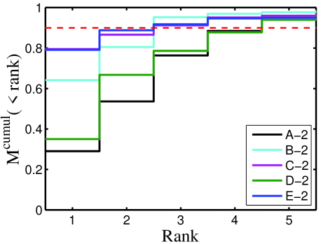
Figure 1: Cumulative stellar mass fractions obtained from our solar neighbourhood-like spheres, centred at 8 kpc from the galactic centre. The step-like cumulative fractions show the contribution from the five most massive contributors to each sphere in rank order. The most massive contributor is ranked as number 1. The red dashed line shows the $90\%$ level.

The Aquarius Project has simulated the formation of six Milky Way-like dark matter haloes in a $\Lambda$CDM cosmology. The simulations were carried out using the parallel Tree-PM code GADGET-3 (an upgraded version of GADGET-2, Springel, 2005). Each halo was first identified in a lower resolution version of the Millennium-II Simulation (Boylan-Kolchin et al., 2009) which was carried out within a periodic box of side 125 h^-1 Mpc in a cosmology with parameters $\Omega_{m}=0.25$, $\Omega_{\Lambda}=0.75$, $\sigma_{8}=0.9$, $n_{s}=1$, and Hubble constant $H_{0}=100~{}h$ km s^-1 Mpc^-1 = 73 km s^-1 Mpc^-1. The haloes were selected to have masses comparable to that of the Milky Way and to be relatively isolated at $z=0$. By applying a multi-mass particle ‘zoom-in’ technique, each halo was re-simulated at a series of progressively higher resolutions. The results presented in this work are based on the simulations with the second highest resolution (Aq-2) available, with a Plummer equivalent softening length of 65.8 pc. In all cases 128 outputs, starting from redshift $z\approx 45$, were stored. In each snapshot, dark matter haloes were identified using a Friends-of-Friends (Davis et al., 1985) algorithm while subhaloes were identified with SUBFIND (Springel et al., 2001). For more details about the simulations, we refer the reader to Springel et al. (2008b, a). The main properties of the resulting haloes are summarised in Table 1. Note that we exclude from our analysis the halo Aq-F. This is due to its assembly history; more than $95\%$ of its accreted stellar halo mass comes from a single galaxy that was accreted very late, at $z\approx 0.7$.

2.2 Semi-analytic model

Table 2: Properties of the distribution of stellar particles inside our “solar neighbourhood” (sn) spheres of 2.5 kpc radius. The first column labels the simulation. From left to right, the columns give the local stellar density, $\rho_{0}$, the number of most significant stellar mass contributors, $N^{\it sn}_{\rm ms}$ (see text) and the three components of the velocity ellipsoid.

Name	$\rho_{0}/10^{4}$	$N_{\rm ms}^{\it sn}$	$\sigma_{R}$	$\sigma_{\phi}$	$\sigma_{Z}$
	[M⊙ kpc-3]		[km s-1]	[km s-1]	[km s-1]
A-2	1.54	5	149.4	130.9	90.5
B-2	15.4	3	85.3	51.1	45.5
C-2	2.55	3	148.2	98.1	80.7
D-2	8.24	5	175.1	88.5	75.7
E-2	3.44	3	93.8	62.3	55.0

To study the growth and properties of stellar haloes, Cooper et al. (2010) coupled the semi-analytic model GALFORM to the Aquarius dark matter $N$-body simulations. The basic idea behind semi-analytic techniques is to model the evolution of the baryonic components of galaxies through a set of observationally and/or theoretically motivated analytic prescriptions. Critical physical processes that govern galaxy formation, such as gas cooling, star formation feedback, supernovae, winds of massive stars and AGN, etc.  are taken into account. The parameters that control these processes were fixed on the basis of an implementation of GALFORM on the Millennium Simulation (Springel et al., 2005), as this set of choices allows one to successfully reproduce the properties of galaxies on large scales as well as those of the Milky Way (Bower et al., 2006; Cooper et al., 2010).

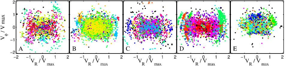
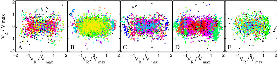
Figure 2: Distribution in $V_{R}$ vs. $V_{\phi}$ (top panels) and $V_{R}$ vs. $V_{Z}$ (bottom panels) space of the stellar particles located inside a sphere of 2.5 kpc radius at 8 kpc from the galactic centre. The different colours represent different satellites. The corresponding host halo is indicated on the lower left corner of each panel.

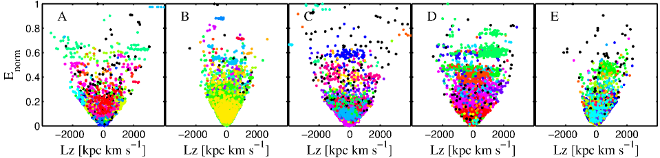
Figure 3: Distribution in $E$ vs. $L_{z}$ space for the same set of particles as shown in Figure 2. The corresponding host halo is indicated on the top left corner of each panel.

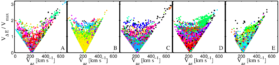
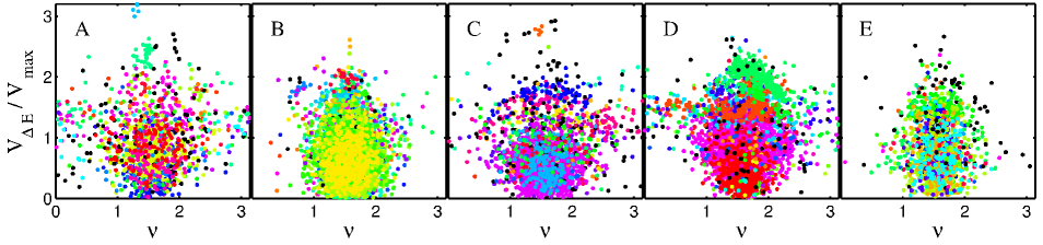
Figure 4: Distribution in $V_{\rm az}$ vs. $V_{\Delta E}$ (top panels) and $\nu$ vs. $V_{\Delta E}$ (bottom panels) space for the set of particles shown in previous figures. The corresponding host halo is indicated on the lower right corner of each panel.

2.3 Building up stellar haloes

Within the context of CDM, stellar haloes may be formed via hierarchical aggregation of smaller objects, each one of them imprinting their own chemical and dynamical signatures on the final halo’s properties (Freeman & Bland-Hawthorn, 2002). As previously explained, the GALFORM model provides a detailed description of the composite stellar population of every galaxy in the simulation at any given time. However it does not follow the dynamics of these systems fully. To study the dynamical properties of the resulting galactic stellar haloes Cooper et al. (2010) assumed that the most strongly bound dark matter particles in progenitor satellites could be used to trace the phase-space evolution of their stars. In every snapshot of the simulation a fixed fraction of the most-bound dark matter particles were selected to trace any newly formed stellar population in each galaxy in the simulation. This implies that each tagged particle has a different final stellar mass associated to it. The fraction of selected bound particles is set such that properties of the satellite population at $z=0$, like their luminosities, surface brightness, half-light radii and velocity dispersions, are consistent with those observed for the Milky Way and M31 satellites. For a detailed description of this procedure we refer the reader to Section 3 of Cooper et al. (2010). The properties of the resulting stellar haloes obtained in each simulation, such as total mass, half-light radius and the root-mean-square (RMS) scatter in the logarithm of the stellar mass assigned to the individual particles are listed in Table 1. Note that, although the method introduced in Cooper et al. (2010) leads to a successful match of various observables regarding the structure and characteristics of the Galactic stellar halo and its satellite population, the dynamical evolution of the baryonic components of galaxies is much simplified. This likely has an effect on e.g. the efficiency of satellite mass loss due to tidal stripping, or the satellite’s internal structural changes due to adiabatic contraction, and possibly even on its final radial distribution. (Libeskind et al., 2010; Romano-Díaz et al., 2010; Schewtschenko & Macciò, 2011; Geen et al., 2013).

3 Characterization of Substructure in solar volumes

In this Section we characterize the phase-space distribution of stellar particles inside a “solar neighbourhood” sphere located at 8 kpc from the galactic centre of each Aquarius stellar halo. Following Gómez et al. (2010), we chose for the spheres a radius of 2.5 kpc as this is approximately the distance within which the astrometric satellite Gaia (Perryman et al., 2001) will be able to provide extremely accurate 6D phase-space measurements for an unprecedentedly large number of stars. The final configuration of the host dark matter haloes is, in all cases, strongly triaxial. Therefore, to allow a direct comparison between the “solar neighbourhood” spheres from different haloes, we have rotated each halo to its set of principal axis and placed the sphere along the direction of the major axis. In all cases, the ratios and directions of the principal axis were computed using dark matter particles located within 6 to 12 kpc.

Table 2 shows that $90\%$ of the total stellar mass enclosed in these spheres comes, in all cases, from 3-5 significant contributors, $N_{\rm ms}^{\it sn}$. This is in agreement with De Lucia & Helmi (2008); Cooper et al. (2010), who find that stellar haloes are predominantly built from fewer than 5 satellites with masses comparable to the brightest classical dwarf spheroidals of the Milky Way. Figure 1 shows the stellar mass fractions contributed by the five most significant contributors to the total stellar mass enclosed in each sphere.

In Figure 2 we present two different projections of velocity space. The different colours indicate particles coming from different satellites that have contributed with at least five particles (while those from satellites contributing fewer particles are shown in black). It is interesting to observe how these distributions in velocity space vary from halo to halo. Essentially, less massive (dark) haloes have smaller velocity dispersions and thus the distribution of particles in velocity space is more compact. The values of the velocity dispersions of these distributions are listed in Table 2. A comparison with the estimated values of the velocity ellipsoid of the local stellar halo (see Chiba & Beers, 2000) $(\sigma_{R},\sigma_{\phi},\sigma_{Z})=(141\pm 11,106\pm 9,94\pm 8)$ km s^-1 shows that the ellipsoids of haloes Aq-A-2, -C-2 and -D-2 have amplitudes comparable to those observed for the Milky Way. Note, however, that the dynamics of the stellar particles in these simulations are only determined by the underlying dark matter halo potential. If the mass associated to the disc and the bulge were to be included, the velocity dispersions would be significantly increased, since we may relate the velocity dispersion $\sigma^{2}$ to the circular velocity $V_{c}^{2}$ and $V_{c}^{2}\propto M(<r)=M_{\rm disc}+M_{\rm halo}$, and $M_{\rm disc}\sim M_{\rm halo}$ near the Sun (Binney & Tremaine, 2008). In Table 2 we also show the local stellar halo average densities, $\rho_{0}$. We find that, except for halo Aq-B-2, the values obtained are in reasonable agreement with the estimates for the Solar Neighbourhood, $\rho_{0}=1.5\times 10^{4}$ M_⊙ kpc^-3 (see, e.g., Fuchs & Jahreiß, 1998). However, one should bear in mind that, if a disc component were to be included, this should lead to a contraction of the halo, and hence to a larger density, especially on the galactic disc plane (e.g., Abadi et al., 2010; Debattista et al., 2008). The highest local density is found for halo Aq-B-2. This halo has a low stellar mass compared to haloes Aq-D-2 and E-2, but is much more centrally concentrated than Aq-D-2. In comparison to Aq-E-2, which is also very centrally concentrated, Aq-B-2 has a strongly prolate shape, which explains its much higher value of $\rho_{0}$ on the major axis, where our “solar neighbourhood” sphere is placed.

From Figure 2 we can also appreciate the very large amount of substructure, coming from many different objects, that is present in these volumes. This substructure, in the form of stellar streams, can be seen as groups of unicoloured star particles. Recall that these stellar haloes are built up in a fully cosmological scenario. Therefore, effects such as violent variation of the host potential due to merger events, and chaotic orbital behaviour induced by the strongly triaxial dark matter haloes (Vera-Ciro et al., 2011) are naturally accounted for in these simulations. Nonetheless, these physical processes have not been efficient enough to completely erase the memory of the origin of the stellar halo particles. Note that, for this analysis, we have treated all tagged particles equally. As described in Section 2.3, the stellar-to-total mass ratio varies from particle to particle. Thus, the relative masses of the identified streams as judged by their particle number could be quite different from their relative stellar mass. We will explore this further in the following Section.

Evidence for this can also be seen in Figure 3, which shows the distribution of stellar particles in the space of the pseudo-conserved quantities $E_{\rm norm}$ and $L_{z}$, where

$$E_{\rm norm}=\dfrac{E-E_{\min}}{E_{\rm max}-E_{\rm min}},$$ (1)

with $E_{\rm max}$ and $E_{\rm min}$ are the energies of the most and the least bound stellar particles inside the volume under analysis, respectively. To compute the energy we assume a smooth and spherical representation of the underlying gravitational potential, as given by Navarro et al. (1996)

$$\Phi(r)=-\frac{GM_{\rm 200}}{r\left[\ln(1+c_{\rm NFW})-c_{\rm NFW}/(1+c_{\rm NFW})\right]}\\ \ln\left(1+\frac{r}{r_{s}}\right),$$ (2)

with values for the parameters at redshift $z=0$ as listed in Table 1. As expected, substructure in this space is much better defined than in velocity space (see also e.g. Helmi & de Zeeuw, 2000; Knebe et al., 2005; Font et al., 2006; Gómez & Helmi, 2010). In this projection of phase-space streams from the same satellite tend to cluster together and can be observed as well defined clumps. Note however that within a given clump substructure associated with the various streams crossing the “solar neighbourhood” may be apparent (see, e.g., Gómez & Helmi, 2010).

To search for stellar streams in the Solar Neighbourhood without assuming an underlying Galactic potential, Klement et al. (2009) introduced the space of $\nu$, $V_{\Delta E}$ and $V_{\rm az}$, where

$$\begin{array}[]{lll}\displaystyle\nu=\arctan\left(\dfrac{V+V_{\rm LSR}}{W}\right),\\ \\ \displaystyle V_{\Delta{\rm E}}=\sqrt{U^{2}+2(V_{\rm LSR}-V_{\rm az})^{2}},\\ \\ \displaystyle V_{\rm az}=\sqrt{(V+V_{\rm LSR})^{2}+W^{2}}.\end{array}$$ (3)

These are based only on kinematical measurements. For a star in the Galactic plane, $\nu$ would be the angle between the orbital plane and the direction towards the North Galactic Pole, $V_{\rm az}$ is related to the angular momentum and $V_{\Delta{\rm E}}$ is a measure of a star’s eccentricity. Under the assumption of a spherical potential and a flat rotation curve, stars in a given stellar stream should be distributed in a clump when projected onto this space. The distribution of stellar particles located inside our “solar neighbourhood” spheres projected onto the spaces of $V_{\rm az}$ vs. $V_{\Delta{\rm E}}$ and $\nu$ vs. $V_{\Delta{\rm E}}$ are shown in Figure 4. Although perhaps less sharply defined than in $E$ vs. $L_{z}$ space, substructure stands out in these two projections of phase-space.

4 Quantification of Substructure in solar volumes

In the previous Section we found that the phase-space distribution of stellar particles inside a “solar neighbourhood” sphere is very rich in substructure in all of our haloes. We will now quantify the number of stellar streams crossing the “solar neighbourhoods” of our Aquarius haloes and characterize their evolution in time. Our goal is to compare the results of this analysis with previous studies (Helmi & White, 1999; Helmi et al., 2003) that have analytically estimated this number and concluded that the merger history of the Milky Way could be recovered from the phase-space distribution of Solar Neighbourhood stars. Furthermore, we will address what fraction of the stellar particles that appear to be smoothly distributed in phase-space are actually in streams that could not be resolved due to the high but limited particle resolution of our $N$-body simulations. We will also establish the importance of chaotic mixing for the quantification of substructure.

4.1 Resolved substructure

To quantify the number of streams inside our spheres we first need to specify how to identify them. Our definition of a stream must ensure that particles in the same stream share the same orbital phase and progenitor. Following Helmi et al. (2003), a stream is identified when i) two or more particles from the same parent satellite are found within one of our 2.5 kpc solar neighbourhood spheres at redshift $z=0$ and ii) they share at least one particle from the same parent satellite that has never been separated by more than a distance $r_{\rm stream}$ from either of them. The value of $r_{\rm stream}$ is set to account for the stellar streams that, due to numerical resolution, are poorly resolved in the “solar neighbourhood”. In this work we adopt $r_{\rm stream}=0.8\times r_{\rm apo}$ for each particle, where $r_{\rm apo}$ is its apocenter at $z=0$, estimated from the outputs of the $N$-body simulations. Varying the value of $r_{\rm stream}$ between $0.6$ - $0.9\times r_{\rm apo}$ did not significantly affect our results. This is required because a parent satellite can contribute with multiple stellar streams that may cross each other in configuration space (see, e.g., Helmi & White, 1999). Note that using $r_{\rm apo}$ as a scale allows us to naturally adapt the algorithm to different orbital configurations.

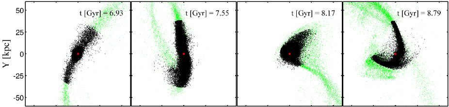
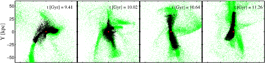
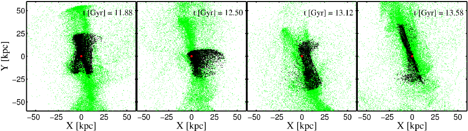
Figure 5: Time evolution of a stellar stream that crosses the “solar neighbourhood” sphere of the Aquarius halo A-2 at redshift $z=0$. The green dots show all the stellar particles from the corresponding parent-satellite. With black dots we show the particles that have always been within $r_{\rm stream}$ from the reference particle (red dot), which is indicated with an arrow in Figure 6.

In practice, we proceed as follows:

• For each particle inside our solar neighbourhood sphere of 2.5 kpc radius at redshift $z=0$ we identify its parent satellite.

• We measure the time $t_{\rm form}$ (prior the time of accretion) when the spatial extent of all particles associated with this parent takes its smallest value (as measured by the root-mean-square dispersion of distance from the centre of mass of the satellite).

• At $t=t_{\rm form}$ we identify all particles located in a sphere of 4 kpc radius, centred on the selected particle. This radius has to be large enough to initially contain all potential neighbouring members of this given particle. We have performed various tests and found the results to be robust to the sphere’s extent.

• We follow these particles forward in time until $z=0$, and discard those that, at any time, are more distant than $r_{\rm stream}$ from the selected particle.

• The selected particle is considered to be in a stream if, at final time, another particle from the same parent satellite can be found within our solar neighbourhood sphere and, moreover, they have in common at least one of the original neighbouring particles lying within their respective $r_{\rm stream}$.

Table 3: Properties of the distribution of particles tagged with stars inside “solar neighbourhood” spheres of 2.5 kpc radius located at 8 kpc from the galactic centre. The first column labels the simulation. From left to right, the remaining columns give the total number of contributing satellites, $N_{\rm sat}^{\it sn}$; the total number of star particles, $n_{*}$; the fraction of star particles in resolved streams; $f_{\rm stream}^{n_{*}}$; the fraction of stellar mass in resolved streams, $f_{\rm stream}^{m_{*}}$; the total number of streams, $N_{\rm stream}$; and the fraction of streams coming from the five most significant stellar mass contributors, $f_{\rm stream}^{5\rm{mm}}$.

Name	$N_{\rm sat}^{\it sn}$	$n_{*}$	$f_{\rm stream}^{n_{*}}$	$f_{\rm stream}^{m_{*}}$	$N_{\rm stream}$	$f_{\rm stream}^{5\rm{mm}}$
A-2	$85$	$1400$	$20.2\%$	$31.1\%$	$83$	$63\%$
B-2	$38$	$10740$	$82.0\%$	$92.4\%$	$582$	$74\%$
C-2	$105$	$2334$	$46.9\%$	$62.7\%$	$223$	$68\%$
D-2	$63$	$3853$	$68.2\%$	$85.5\%$	$301$	$65\%$
E-2	$53$	$1957$	$36.7\%$	$62.7\%$	$125$	$84\%$

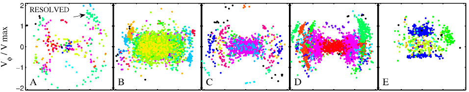
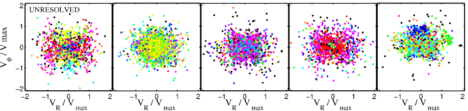
Figure 6: Distribution in $V_{R}$ vs. $V_{\phi}$ space of the stellar particles located inside a sphere of 2.5 kpc radius centred at 8 kpc from the galactic centre. The corresponding host halo is indicated on the lower left corner of the top panels. The top panels show the distribution of particles that were linked to stellar streams (resolved component) whereas the bottom panels the remaining particles (unresolved component). As in Figure 2, different colours indicate different satellites. The arrow in top left panel of this figure indicates the stream that is shown in Figure 5.

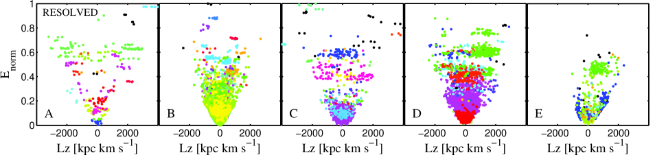
Figure 7: Distribution in $E$ vs. $L_{z}$ space of the stellar particles that were linked to stellar streams (resolved component) located inside a sphere of 2.5 kpc radius centred at 8 kpc from the galactic centre. The corresponding host halo is indicated on the lower left corner of the top panels. The colour coding is the same as in the top panel of Figure 6.

Figure 5 shows, as an example, the time evolution of one of the streams crossing the “solar neighbourhood” of the halo Aq-A-2, at $z=0$. The corresponding progenitor is the second most massive contributor to the stellar halo and, prior accretion, it had a stellar mass of $\approx 1.25\times 10^{8}$ M_⊙. Its redshift of infall is $z\approx 2.3$ and by $z=0$ it has been fully disrupted. The stream is indicated with an arrow in Figure 6. The black dots correspond to the particles that have always been neighbours (i.e. within $r_{\rm stream}$) of a reference particle in this stream, which is indicated with a red dot. This figure clearly shows the full spatial extent of the stream, which probes regions far beyond the “solar neighbourhood” volume.

The numbers of streams with at least two particles found inside the “solar neighbourhood” spheres located at 8 kpc from the galactic centre are listed in Table 3. These numbers are well in the range of the $\sim$ 300 - 500 stellar streams around the Sun predicted by the models of Helmi & White (1999) (see also Gómez et al., 2010). Halo Aq-A-2 has the smallest number of resolved streams, as well as the lowest fraction of particles associated with them (see Table 3), and the largest associated particle fraction are found in halo Aq-B-2. Table 3 also shows the total number of accreted particles found within each sphere as well as the total number of progenitor satellites that have contributed them. Note that the fraction of stellar mass in resolved streams is always larger than the fraction of star particles in resolved streams. Thus, the star particles with high stellar-to-total mass ratio, which come from the denser and inner parts of the original satellites, are more likely to be found in resolved streams.

From this table we see that disrupted satellites contribute many more star particles at 8 kpc in Aq-B-2 than in the other haloes, and as a result the streams are much better resolved. The next best resolved “solar neighbourhood” is found in Aq-D-2. For the other haloes, a significant fraction of the particles have not been associated with any substructure and, therefore the total number of streams (which would include those unresolved), could be significantly larger. We will explore this further in Section 4.2.

In Figure 6 we compare the velocity distributions of stellar particles in streams (top panels) to those not associated with any structure (bottom panels) according to our algorithm. Different columns correspond to distributions of stellar particles inside “solar neighbourhoods” of different haloes. As in Figure 2, the different colours represent different satellites. In addition to a very large number of inconspicuous substructures, we can see that the most prominent streams have been recovered in all cases. Note that the particles in streams tend to populate the wings of the distribution. In general, particles in the core of the velocity distribution will have been accreted earlier and tend to have shorter periods (and hence to mix faster). Therefore, streams will be more difficult to identify because of the limited resolution. In addition, and as explained below, it is possible that due to the triaxiality of the dark matter potential some of these orbits exhibit chaotic mixing. The associated streams would then be too convoluted to be observable. Note, however, that thanks to the much larger number of star particles and the smaller velocity dispersion (see Section 3), a significant fraction of the particles in the core of the distribution for Aq-B-2 are in resolved streams. Figure 7 shows the distribution of stellar particles in streams in integrals of motion space. Substructure in this space is clearly visible. We emphasise that this is the case even in the presence of violent variation of the host potential due to merger events and chaotic orbital behaviour induced by the strongly triaxial dark matter haloes.

In the top panel of Figure 8 we explore how the number of streams found inside spheres of 2.5 kpc radius changes as a function of galactocentric distance along the direction of the major axis. It is interesting to see that in all cases the number of streams decreases as a power-law with radius. Note, however, that haloes Aq-B-2 and E-2 have steeper profiles than the other haloes. As described by Cooper et al. (2010), the majority of the stellar mass in these two cases comes from one or two objects that deposit most of their mass in the inner regions of the haloes. Interestingly, these two haloes have the largest fraction of streams coming from the five most significant stellar mass contributor (see Table 3). As shown in the bottom panel of Figure 8, the same behaviours is observed in the local density profiles of these haloes, $\rho_{0}(r)$, measured along the major axis. Note that, due to the triaxial nature of the resulting haloes, varying azimuthally the location of our spheres results in local stellar densities that are, in general, an order of magnitude smaller than the observed value in the Solar Neighbourhood. For example, at a distance of 8 kpc along the intermediate axis, halo Aq-A-2 has $\rho_{0}=4.9\times 10^{3}$ M_⊙ kpc³ and a total number of streams $N_{\rm streams}=37$. An isodensity contour defined by the value of $\rho_{0}$ at 8 kpc along the major axis places the solar neighbourhood-like sphere at distance of $\approx 4$ kpc on the intermediate axis. At this location $N_{\rm streams}$ raises to 68, indicating that azimuthal variations in the number of streams mainly reflect changes in local stellar density.

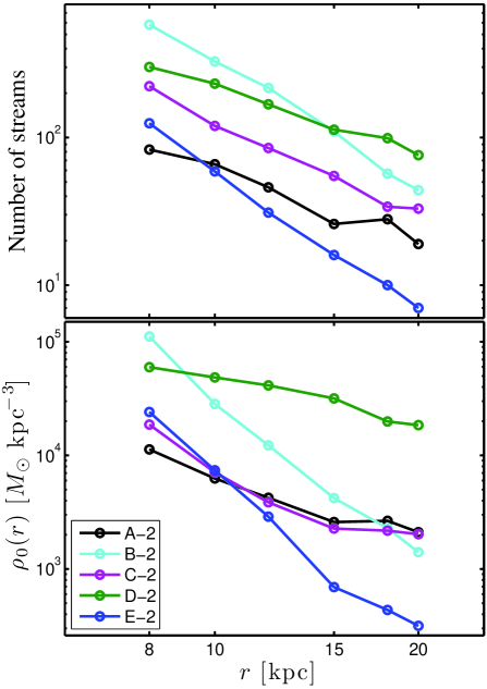
Figure 8: Top panel: Number of streams as a function of galactocentric radius found within spheres of 2.5 kpc radii. Bottom panel: Spherically averaged stellar density profiles. The different colours indicate different haloes.

4.2 Smooth/Unresolved component

In addition to the stellar particles associated with streams with at least two particles, our “solar neighbourhood” spheres contain an important number of stellar particles that are not linked to any substructure, i.e., they appear to be smoothly distributed in phase-space. The reason for this could be either of dynamical origin or, as posited before, simply due to the numerical resolution of the simulation. It is well known that phase-space regions of triaxial dark matter haloes may exist that are occupied by chaotic orbits (e.g., Vogelsberger et al., 2008). On such orbits, stellar particles that are initially nearby diverge in space exponentially with time. As a result, substructure that is present in localised volumes of phase-space left by accretion events is rapidly erased. This process is known as chaotic mixing. On the other hand, initially nearby particles in phase-space on regular orbits diverge in space as a power-law in time. Therefore, the time-scale in which these particles fully phase-mix may be much larger.

Based on the previous discussion, we will now analyse the evolution in time of the local (stream) density around the particles found at the present day in each “solar neighbourhood” sphere. Our goal is to assess the influence of chaotic mixing on the underlying phase-space distributions and to estimate the fraction of particles that, due to the high but nonetheless limited numerical resolution of our simulations, were not associated with any stream.

As in Section 4.1, we place a sphere of 4 kpc radius around each particle at $t=t_{\rm form}$ and tag all the surrounding neighbours. We track these particles forward in time until redshift $z=0$ and those neighbours that depart from our particles by more than $r_{\rm stream}$ at any time are discarded. We compute the local spatial density of the selected particle, $\rho(t)$, by counting the number of neighbours within a distance $r_{\rm dens}=0.5\times r_{\rm apo}$. In Figure 9 we show the time evolution of the spatial density of particles from two different satellites that contribute to the “solar neighbourhood” of the halo Aq-A-2. From this figure we can appreciate that the rate at which the spatial density of a stream decreases with time varies strongly (likely as a consequence of the different orbits). We can also observe that in many cases, when a particle becomes unbound from its parent satellite, the density of the newly formed stream exhibits initially a very rapid and quasi-exponential decrease. As shown by Gómez (2010) (see also Helmi & Gomez, 2007), this initial transient is also present in regular orbits and does not necessarily imply a manifestation of chaotic behaviour. It is therefore necessary to follow the evolution of the stream’s density for long time scales (much longer than a crossing time) to disentangle regular from chaotic behaviour.

Our approach to characterizing the type of mixing consists in fitting a power-law function to the time evolution of the local density of a stream,

$$\hat{\rho}(t)=\alpha t^{-n},$$ (4)

and determining the value of $n$ for each stream. As shown by Vogelsberger et al. (2008) (see also Helmi & White, 1999) for a stream on a regular orbit, $n=1$, 2 or 3 depending on the number of fundamental orbital frequencies. Although we know that the density of a stream on a chaotic orbit does not evolve as a power law in time, we nonetheless fit the functional form given by Eq. (4), and expect larger values of $n$ than for the regular case. We warn the reader that, given our simple approach, the resulting distributions of $n$-values should be considered as an estimate of the rate at which diffusion is acting in a given volume, rather than a precise characterization of the underlying phase-space structure.

Figure 9 shows the results of applying such a fit to the stream densities as a function of time. Since we are interested in the behaviour of the density on long time scales, we do not include the initial quasi-exponential transient in the fits. We proceed as follows:

• We define the formation time of a stream, $t_{\rm stream}$, as the time when its density decreases from one snapshot to the next one by $50\%$.

• Starting from the snapshot associated with $t_{\rm stream}$, we iteratively fit ten times a power-law function to the stream’s density by increasing in each iteration the starting time snapshot by snapshot. The fits are always normalized to the value of the density at the starting point. Furthermore, each data point is weighted according to the number of particles used to measure the corresponding density.

• We estimate the goodness of each fit by computing the root mean squared error, $RMSE$, defined as:

  $$RMSE=\sqrt{\dfrac{\sum_{i=1}^{m}\left(\hat{\rho}(t_{i})-\rho(t_{i})\right)^{2}}{m-2}}$$ (5)

  where $\rho(t_{i})$ is the density estimated from the particle count and $m$ is the number of data points used in the fit.

• Of all these experiments, we only keep the value of $n$ obtained from the fit where the $RMSE$ is smallest.

The results of applying this procedure to all the particles inside 2.5 kpc radius spheres of different haloes are shown in Figure 10. We explore spheres located at three different galactocentric radii, namely 8 , 15 and 20 kpc. The black solid histograms show the distribution of $n$-values for all the particles in each “solar neighbourhood” sphere. At ${\rm R}=8$ kpc (top panels), with the exception of haloes Aq-B-2 and E-2, we find narrow distributions peaking at values slightly larger than $n=3$. Note, however, that as we move outward from the galactic centre, the peak of all distributions tend to shift towards values much closer to $n=3$. A clear example is halo Aq-B-2, where the peak of the distribution shifts from $n\approx 7$ at ${\rm R}=8$ kpc to $n\lessapprox 3$ at ${\rm R}=20$ kpc (bottom panel).

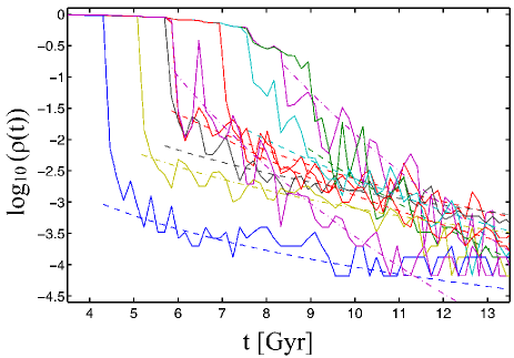
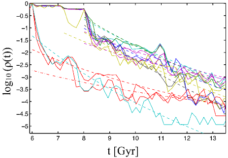
Figure 9: Time evolution of the density of streams originating in two different satellites that contribute, at redshift $z=0$, to the solar neighbourhood sphere obtained from halo Aq-A-2. Each panel corresponds to a different satellite. The dashed lines show the power-law fits applied to the particles identified as stream members, as explained in Section 4.2, whereas the dashed-dotted lines correspond to the remaining particles.

Figure 10 also shows in black dashed histograms the distribution $n$-values for those particles associated with “resolved” stellar streams, while the grey-dashed histograms correspond to the remaining particles. From this figure we can observe that although the two distributions overlap significantly, there is a clear offset between them. In each panel we show the median values of $n$, $\tilde{n}$. Stellar particles in streams (which are more likely to be on regular orbits) tend to have the smallest values of $n$ and, in general, their distribution peaks at a value much closer to $n=3$ than their unresolved counterparts. Let us recall that this is the value of $n$ expected for the dependence of density on time for regular orbits in a three dimensional time independent gravitational potential (see, e.g. Helmi & White, 1999; Vogelsberger et al., 2008).

It is interesting to compare the $n$-distributions obtained from haloes Aq-A-2 and B-2 at ${\rm R}=8$ kpc. As previously discussed, while halo B-2 has the largest number of streams and the greatest fraction of accreted particles associated with them, the opposite is found for halo Aq-A-2. The value of $\tilde{n}\approx 7$ obtained from the resolved component in halo B-2 suggests that these particles are undergoing chaotic mixing. Nonetheless, thanks to the high particle resolution, substructure can be efficiently identified. Note the large difference between the medians obtained from the resolved and unresolved components. For halo Aq-A-2 , the distribution of $n$-values associated with the two components show a very similar value of $\tilde{n}\approx 4.3$, considerably closer to what is expected for regular orbits. This suggests that a significant fraction of the particles that have not been associated with streams are on (nearly) regular orbits, and that because of the limited numerical resolution, they are not found in (massive) streams.

Interestingly, we find that, on average, particles in resolved streams in Aq-A-2 were released from their parent satellite 2.5 Gyr later and have more extended orbits than the particles in the unresolved component. The average apocentric distances for these two subsets are 32 and 12 kpc, respectively. Thus, the shorter orbital periods and longer times since release partially explain why the latter are not found to be part of (massive) streams. A lower limit to the fraction of accreted particles in resolved stellar streams, corrected by resolution effects, can be obtained by quantifying the fraction of particles in the unresolved component with $n$-values smaller than the median of the resolved component, $\tilde{n}_{\rm res}$. We find in halo Aq-A-2 a total of 411 particles that satisfy this condition. In addition to the 283 particles associated with the resolved component, we estimate that at least $50\%$ of all accreted particles in this halo should be part of a resolved stellar stream. Furthermore, the corresponding stellar mass fraction should at least be as large as $65.7\%$.

In general, particles in resolved streams were released later (than those in the unresolved component) for all haloes. We find for haloes Aq-B-2, C-2, D-2 and E-2 a time difference of 1.9, 1, 2.2, and 2 Gyr, respectively. However, differences in the mean apocentric distances are found only in halo Aq-A-2. As for halo Aq-A-2, we can obtain for the remaining haloes an estimate for the lower limit of particles in resolved stellar streams corrected by resolution effects. We find a total of $(380,348,268,350)$ particles with $n$-values smaller than $\tilde{n}_{\rm res}$ in haloes (B-2, C-2, D-2, E-2), respectively. Thus, we estimate that the corresponding fractions of particles and stellar mass in resolved streams for these haloes should be, at least, as large as $(55\%,75\%,62\%,84\%)$ and $(96\%,80\%,91\%,84\%)$, respectively.

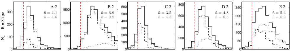
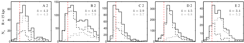
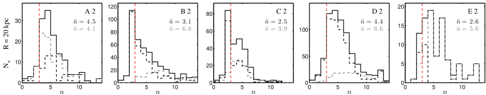
Figure 10: The black solid histograms show the distribution of $n$-values found for particles in “solar neighbourhood” spheres of 2.5 kpc radius. Each column corresponds to a different satellite. Different rows corresponds to volumes centred at different galactocentric radius. The black (respectively grey) dashed histograms correspond to those particles that are (respectively, not) associated to resolved stellar streams. The vertical red dashed line is located at $n=3$. For regular orbits, $n\leq 3$ is expected. Each panel shows the median values $\tilde{n}$, obtained from the distributions for particles in resolved and in unresolved streams.

5 Summary

In this work we have characterized the phase-space distribution as well as the time evolution of debris for stars found inside “solar neighbourhood” volumes. Our analysis is based on simulations of the formation of galactic stellar haloes, as described by Cooper et al. (2010). The haloes were obtained by combining the very high resolution fully cosmological $\Lambda$CDM simulations of the Aquarius project with a semi-analytic model of galaxy formation.

We find that, for haloes Aq-A-2, -C-2 and -D-2, the measured velocity ellipsoid at 8 kpc on the major axis of the halo is in good agreement with the estimate for the local Galactic stellar halo (Chiba & Beers, 2000). Similarly, for all haloes but Aq-B-2, the local stellar halo average density on the major axis is in reasonable agreement with the observed value (Fuchs & Jahreiß, 1998). However, we note that if the contribution of the disc and bulge were to be included, the resulting velocity dispersions as well as the local stellar halo average density would be significantly increased. This could suggest that these dark haloes are too massive to host the Milky Way (in agreement with Battaglia et al., 2005; Sales et al., 2007; Smith et al., 2007; Wang et al., 2012; Vera-Ciro et al., 2013). On the other hand, if located in a prolate low mass halo such as Aq-B-2, the measured local stellar density would imply that the Sun should be on the intermediate or minor axis, i.e. the Galactic disc’s angular momentum would be aligned with the major axis of the dark halo (Helmi, 2004). On the minor axis, haloes B and E have velocity ellipsoids of smaller amplitude and hence could perhaps be made consistent with those observed near the Sun, if the effects of the contraction induced by the disc were taken into account. However, for haloes A, C, and D, the dispersions on the minor axis are larger than those on the major axis at the equivalent of the solar circle.

In agreement with previous work, we find that $90\%$ of the stellar mass enclosed in our “solar neighbourhoods” comes, in all cases, from 3 to 5 significant contributors. These “solar neighbourhood” volumes contain a large amount of substructure in the form of stellar streams. In the five analysed stellar haloes, substructure can be easily identified as kinematically cold structures, as well as in well defined lumps of stellar particles in spaces of pseudo-conserved quantities.

By applying a simple algorithm to follow the time evolution of local densities in the neighbourhood of reference particles, we have quantified the number of (massive) streams that can be resolved in solar neighborhood-like volumes. In haloes where solar neighbourhood-like volumes are best resolved we find that the number of resolved streams is in very good agreement with the predictions given by Helmi & White (1999). As we move outward from the galactic centre the number of streams decreases as a power-law, in a similar fashion to the density profiles.

To explore whether the halo-to-halo scatter in the total number of resolved streams is due to poor particle resolution or to chaotic mixing, we have estimated the rate at which local (stream) densities decrease with time. Interestingly, we find that in our best-resolved solar neighbourhood-like volume (Aq-B-2) a large amount of substructure can be identified, even in the presence of chaotic mixing. In this halo, up to $82\%$ of the star particles (and $92\%$ of the stellar mass) can be associated with a resolved stream. On the other hand, our poorest-resolved solar neighbourhood-like volume (Aq-A-2) shows a smaller amount of substructure but significantly longer mixing time-scales (a rate that is close to what is expected from regular orbits). In this case, only $20\%$ of the accreted star particles (and $31\%$ of the accreted stellar mass) can be linked to streams. A comparison of the orbital properties of resolved and unresolved stream-populations shows that, in general, particles in resolved streams are released later and have longer orbital periods. Moreover, diffusion in both populations occurs at very similar rates. Thus, this analysis suggests that our strongest limitation to quantifying substructure is mass resolution rather than diffusion due to chaotic mixing. We have estimated a lower limit to the fraction of accreted particles in resolved stellar streams by correcting for resolution effects. We find that this fraction should be, at least, as large as $50\%$ by number and $65\%$ by stellar mass in all haloes.

The results presented in this work suggest that the phase-space structure in the vicinity of the Sun should be quite rich in substructure. Recall that our analysis is based on fully cosmological simulations and therefore chaos and violent changes in the gravitational potential that are so characteristic of cold dark matter model, are naturally included.

With the imminent launch of the astrometric satellite Gaia (Perryman et al., 2001), we will be able for the first time to robustly quantify the amount of substructure in the form of stellar streams present within $\approx 2$ kpc from the Sun. This mission from the European Space Agency will provide accurate measurements of positions, proper motions, parallaxes and radial velocities of an unprecedentedly large number of stars. In addition, recent and ongoing surveys such as SEGUE (Yanny et al., 2009), RAVE (Steinmetz et al., 2006), LAMOST (Cui et al., 2012), HERMES (Barden et al., 2010) and Gaia-ESO (Gilmore et al., 2012) will allow us to complement these Gaia observations. A direct comparison of the degree of substructure found in the Solar Neighbourhood with that found in numerical models such as those presented here will allow us to establish directly, for example, how much of the stellar halo has been accreted and how much has been formed in-situ.

References

- Abadi et al. (2010) Abadi M. G., Navarro J. F., Fardal M., Babul A., Steinmetz M., 2010, MNRAS, 407, 435
- Allgood et al. (2006) Allgood B., Flores R. A., Primack J. R., Kravtsov A. V., Wechsler R. H., Faltenbacher A., Bullock J. S., 2006, MNRAS, 367, 1781
- Barden et al. (2010) Barden S. C. et al., 2010, in Society of Photo-Optical Instrumentation Engineers (SPIE) Conference Series, Vol. 7735, Society of Photo-Optical Instrumentation Engineers (SPIE) Conference Series
- Battaglia et al. (2005) Battaglia G. et al., 2005, MNRAS, 364, 433
- Beers et al. (2012) Beers T. C. et al., 2012, ApJ, 746, 34
- Belokurov et al. (2007) Belokurov V. et al., 2007, ApJ, 658, 337
- Belokurov et al. (2006) Belokurov V. et al., 2006, ApJL, 642, L137
- Binney & Tremaine (2008) Binney J., Tremaine S., 2008, Galactic Dynamics: Second Edition. Princeton University Press
- Bond et al. (2010) Bond N. A. et al., 2010, ApJ, 716, 1
- Bower et al. (2006) Bower R. G., Benson A. J., Malbon R., Helly J. C., Frenk C. S., Baugh C. M., Cole S., Lacey C. G., 2006, MNRAS, 370, 645
- Boylan-Kolchin et al. (2009) Boylan-Kolchin M., Springel V., White S. D. M., Jenkins A., Lemson G., 2009, MNRAS, 398, 1150
- Breddels et al. (2010) Breddels M. A. et al., 2010, A&A, 511, A90
- Bryan et al. (2012) Bryan S. E., Mao S., Kay S. T., Schaye J., Dalla Vecchia C., Booth C. M., 2012, MNRAS, 422, 1863
- Bullock & Johnston (2005) Bullock J. S., Johnston K. V., 2005, ApJ, 635, 931
- Burnett et al. (2011) Burnett B. et al., 2011, A&A, 532, A113
- Carollo et al. (2010) Carollo D. et al., 2010, ApJ, 712, 692
- Chiba & Beers (2000) Chiba M., Beers T. C., 2000, AJ, 119, 2843
- Cole et al. (1994) Cole S., Aragon-Salamanca A., Frenk C. S., Navarro J. F., Zepf S. E., 1994, MNRAS, 271, 781
- Cole et al. (2000) Cole S., Lacey C. G., Baugh C. M., Frenk C. S., 2000, MNRAS, 319, 168
- Cooper et al. (2010) Cooper A. P. et al., 2010, MNRAS, 406, 744
- Cui et al. (2012) Cui X.-Q. et al., 2012, Research in Astronomy and Astrophysics, 12, 1197
- Davis et al. (1985) Davis M., Efstathiou G., Frenk C. S., White S. D. M., 1985, ApJ, 292, 371
- De Lucia & Helmi (2008) De Lucia G., Helmi A., 2008, MNRAS, 391, 14
- Debattista et al. (2008) Debattista V. P., Moore B., Quinn T., Kazantzidis S., Maas R., Mayer L., Read J., Stadel J., 2008, ApJ, 681, 1076
- Eggen et al. (1962) Eggen O. J., Lynden-Bell D., Sandage A. R., 1962, ApJ, 136, 748
- Font et al. (2006) Font A. S., Johnston K. V., Bullock J. S., Robertson B. E., 2006, ApJ, 646, 886
- Freeman & Bland-Hawthorn (2002) Freeman K., Bland-Hawthorn J., 2002, ARA&A, 40, 487
- Fuchs & Jahreiß (1998) Fuchs B., Jahreiß H., 1998, A&A, 329, 81
- Geen et al. (2013) Geen S., Slyz A., Devriendt J., 2013, MNRAS, 429, 633
- Gilmore et al. (2012) Gilmore G. et al., 2012, The Messenger, 147, 25
- Gómez (2010) Gómez F. A., 2010, PhD thesis, University of Groningen
- Gómez & Helmi (2010) Gómez F. A., Helmi A., 2010, MNRAS, 401, 2285
- Gómez et al. (2010) Gómez F. A., Helmi A., Brown A. G. A., Li Y.-S., 2010, MNRAS, 408, 935
- Grillmair (2006) Grillmair C. J., 2006, ApJL, 645, L37
- Helmi (2004) Helmi A., 2004, ApJL, 610, L97
- Helmi (2008) Helmi A., 2008, A&AR, 15, 145
- Helmi & de Zeeuw (2000) Helmi A., de Zeeuw P. T., 2000, MNRAS, 319, 657
- Helmi & Gomez (2007) Helmi A., Gomez F., 2007, ArXiv e-prints
- Helmi & White (1999) Helmi A., White S. D. M., 1999, MNRAS, 307, 495
- Helmi et al. (1999) Helmi A., White S. D. M., de Zeeuw P. T., Zhao H., 1999, Nature, 402, 53
- Helmi et al. (2003) Helmi A., White S. D. M., Springel V., 2003, MNRAS, 339, 834
- Ibata et al. (2001) Ibata R., Lewis G. F., Irwin M., Totten E., Quinn T., 2001, ApJ, 551, 294
- Ibata et al. (1994) Ibata R. A., Gilmore G., Irwin M. J., 1994, Nature, 370, 194
- Ibata et al. (2003) Ibata R. A., Irwin M. J., Lewis G. F., Ferguson A. M. N., Tanvir N., 2003, MNRAS, 340, L21
- Klement et al. (2009) Klement R. et al., 2009, ApJ, 698, 865
- Knebe et al. (2005) Knebe A., Gill S. P. D., Kawata D., Gibson B. K., 2005, MNRAS, 357, L35
- Libeskind et al. (2010) Libeskind N. I., Yepes G., Knebe A., Gottlöber S., Hoffman Y., Knollmann S. R., 2010, MNRAS, 401, 1889
- McMillan & Binney (2008) McMillan P. J., Binney J. J., 2008, MNRAS, 390, 429
- Monachesi et al. (2013) Monachesi A. et al., 2013, ApJ, 766, 106
- Morrison et al. (2009) Morrison H. L. et al., 2009, ApJ, 694, 130
- Navarro et al. (1996) Navarro J. F., Frenk C. S., White S. D. M., 1996, ApJ, 462, 563
- Newberg et al. (2002) Newberg H. J. et al., 2002, ApJ, 569, 245
- Perryman et al. (2001) Perryman M. A. C. et al., 2001, A&A, 369, 339
- Romano-Díaz et al. (2010) Romano-Díaz E., Shlosman I., Heller C., Hoffman Y., 2010, ApJ, 716, 1095
- Sales et al. (2007) Sales L. V., Navarro J. F., Abadi M. G., Steinmetz M., 2007, MNRAS, 379, 1464
- Schewtschenko & Macciò (2011) Schewtschenko J. A., Macciò A. V., 2011, MNRAS, 413, 878
- Schlaufman et al. (2011) Schlaufman K. C., Rockosi C. M., Lee Y. S., Beers T. C., Allende Prieto C., 2011, ApJ, 734, 49
- Searle & Zinn (1978) Searle L., Zinn R., 1978, ApJ, 225, 357
- Smith et al. (2009) Smith M. C. et al., 2009, MNRAS, 399, 1223
- Smith et al. (2007) Smith M. C. et al., 2007, MNRAS, 379, 755
- Springel (2005) Springel V., 2005, MNRAS, 364, 1105
- Springel et al. (2008a) Springel V. et al., 2008a, MNRAS, 391, 1685
- Springel et al. (2008b) Springel V. et al., 2008b, Nature, 456, 73
- Springel et al. (2005) Springel V. et al., 2005, Nature, 435, 629
- Springel et al. (2001) Springel V., White S. D. M., Tormen G., Kauffmann G., 2001, MNRAS, 328, 726
- Starkenburg et al. (2009) Starkenburg E. et al., 2009, ApJ, 698, 567
- Steinmetz et al. (2006) Steinmetz M. et al., 2006, AJ, 132, 1645
- Tissera et al. (2012) Tissera P. B., White S. D. M., Scannapieco C., 2012, MNRAS, 420, 255
- Valluri et al. (2010) Valluri M., Debattista V. P., Quinn T., Moore B., 2010, MNRAS, 403, 525
- Valluri et al. (2013) Valluri M., Debattista V. P., Stinson G. S., Bailin J., Quinn T. R., Couchman H. M. P., Wadsley J., 2013, ApJ, 767, 93
- Vera-Ciro et al. (2013) Vera-Ciro C. A., Helmi A., Starkenburg E., Breddels M. A., 2013, MNRAS, 428, 1696
- Vera-Ciro et al. (2011) Vera-Ciro C. A., Sales L. V., Helmi A., Frenk C. S., Navarro J. F., Springel V., Vogelsberger M., White S. D. M., 2011, MNRAS, 416, 1377
- Vogelsberger et al. (2008) Vogelsberger M., White S. D. M., Helmi A., Springel V., 2008, MNRAS, 385, 236
- Wang et al. (2012) Wang J., Frenk C. S., Navarro J. F., Gao L., Sawala T., 2012, MNRAS, 424, 2715
- Williams et al. (2011) Williams M. E. K. et al., 2011, ApJ, 728, 102
- Yanny et al. (2003) Yanny B. et al., 2003, ApJ, 588, 824
- Yanny et al. (2009) Yanny B. et al., 2009, AJ, 137, 4377
- Zwitter et al. (2010) Zwitter T. et al., 2010, A&A, 522, A54