Towards an understanding of jet substructure

Abstract

We present first analytic, resummed calculations of the rates at which widespread jet substructure tools tag QCD jets. As well as considering trimming, pruning and the mass-drop tagger, we introduce modified tools with improved analytical and phenomenological behaviours. Most taggers have double logarithmic resummed structures. The modified mass-drop tagger is special in that it involves only single logarithms, and is free from a complex class of terms known as non-global logarithms. The modification of pruning brings an improved ability to discriminate between the different colour structures that characterise signal and background. As we outline in an extensive phenomenological discussion, these results provide valuable insight into the performance of existing tools and help lay robust foundations for future substructure studies.

1 Introduction

The Large Hadron Collider (LHC) at CERN is increasingly exploring phenomena at energies far above the electroweak scale. One of the features of this exploration is that analysis techniques developed for earlier colliders, in which electroweak-scale particles could be considered “heavy”, i.e. slow-moving, have to be fundamentally reconsidered at the LHC. In particular, in the context of jet-related studies, the large boost of electroweak bosons and top quarks causes their hadronic decays to become collimated inside a single jet. Consequently a vibrant research field has emerged in recent years, investigating how best to identify the characteristic substructure that appears inside the single “fat” jets from electroweak scale objects, as reviewed in Refs. Boost2010 ; Boost2011 ; PlehnSpannowsky . In parallel, the “tagging” and “grooming” methods that have been developed have started to be tested and applied in numerous experimental analyses (e.g. Refs ATLAS:2012am ; Aad:2012meb ; Aad:2013gja ; CMS-substructure-studies for studies on QCD jets and Refs  Aad:2012raa ; Aad:2012dpa ; ATLAS:2012dp ; ATLAS:2012ds ; Chatrchyan:2012ku ; Chatrchyan:2012cx ; Chatrchyan:2012yxa for searches).

The taggers’ and groomers’ action is twofold: they aim to suppress or reshape backgrounds, while retaining signal jets and enhancing their characteristic jet-mass peak at the $W/Z/$Higgs/top/etc. mass. Nearly all the theoretical discussion of these aspects has taken place in the context of Monte Carlo simulation studies (see for instance Ref. Boost2011 and references therein), with tools such as Herwig Herwig6 ; Herwig++ , Pythia Pythia6 ; Pythia8 and Sherpa Sherpa . While Monte Carlo simulation is a powerful tool, its intrinsic numerical nature can make it difficult to extract the key characteristics of individual substructure methods and understand the relations between them. As an example of the kind of statements that exist about them in the literature, we quote from the Boost 2010 proceedings:

The [Monte Carlo] findings discussed above indicate that while [pruning, trimming and filtering] have qualitatively similar effects, there are important differences. For our choice of parameters, pruning acts most aggressively on the signal and background followed by trimming and filtering.

While true, this brings no insight about whether the differences are due to intrinsic properties of the substructure methods analysed or instead due to the particular parameters that were chosen; nor does it allow one to understand whether any differences are generic, or restricted to some specific kinematic range, e.g. in jet transverse momentum. Furthermore there can be significant differences between Monte Carlo simulation tools and among tunes (see e.g. Boost2011 ; Richardson:2012bn ; ATLAS:2012am ; CMS-substructure-studies ), which may be hard to diagnose experimentally, because of the many kinds of physics effects that contribute to the jet structure (final-state showering, initial-state showering, underlying event, hadronisation, etc.). Overall, this points to a need to carry out analytical calculations to understand the interplay between tagging/grooming techniques and the quantum chromodynamical (QCD) showering that occurs in both signal and background jets.

So far there have been three main investigations into the analytical features that emerge from substructure techniques. Refs. Rubin:2010fc ; Rubin:2010boa investigated the mass resolution that can be obtained on signal jets and how to optimize the parameters of a method known as filtering Butterworth:2008iy . Ref. Walsh:2011fz discussed constraints that might arise if one is to apply Soft Collinear Effective Theory (SCET) to jet substructure calculations. Ref. Feige:2012vc observed that for narrow jets the distribution of the $N$-subjettiness shape variable Thaler:2010tr for 2-body signal decays can be resummed to high accuracy insofar as it is related to the thrust distribution in $e^{+}e^{-}$ Catani:1992ua ; Becher:2008cf ; GehrmannDeRidder:2007bj ; Weinzierl:2008iv , though for phenomenological purposes this still needs to be supplemented with a calculation of the interplay with practical cuts on the jet mass. Other calculations that relate to the field of jet substructure include those of planar flow Field:2012rw , energy-energy correlations Larkoski:2013eya and jet multiplicities in the small-jet-radius limit Gerwick:2012fw . Additionally Ref. QuirogaArias:2012nj has examined the extent to which simple approximations about the kinematics involved in tagging and grooming can bring insight into different methods.

Here we embark on a comparative, analytical study of multiple commonly-used taggers and groomers. Ideally we would include all existing methods for both background (QCD jet) and signal-induced jets, however given the many techniques that have been proposed, this would be a gargantuan task. In practice we find that a background-only study, for just a handful of substructure techniques, already brings significant insight into the way the taggers function.

The three commonly used methods that we concentrate on are: the mass-drop tagger (MDT) Butterworth:2008iy , pruning Ellis:2009me ; Ellis:2009su and trimming Krohn:2009th . They all involve the identification of subjets within an original jet, and share the characteristic that they attempt to remove subjets carrying less than some (small) fraction of the original jet’s momentum.

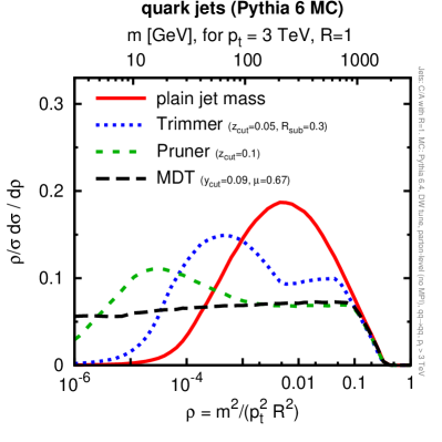
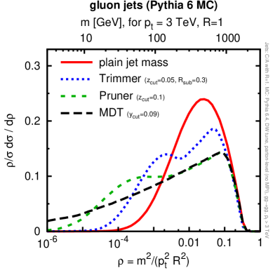
Figure 1: The distribution of $\rho=m^{2}/(p_{t}^{2}R^{2})$ for tagged jets, with three taggers/groomers: trimming, pruning and the mass-drop tagger (MDT). The results have been obtained from Monte Carlo simulation with Pythia 6.425 Pythia6 in the DW tune DW (virtuality-ordered shower), with a minimum $p_{t}$ cut in the generation of $3\,\mathrm{TeV}$, for $14\,\mathrm{TeV}$ $pp$ collisions, at parton level, including initial and final-state showering, but without the underlying event (multiple interactions). The left-hand plot shows $qq\to qq$ scattering, the right-hand plot $gg\to gg$ scattering. In all cases, the taggers have been applied to the two leading Cambridge/Aachen Dokshitzer:1997in ; Wobisch:1998wt jets ($R=1.0$). The parameters chosen for mass-drop ($y_{\text{cut}}=0.09$, $\mu=0.67$), pruning ($z_{\text{cut}}=0.1$, $R_{\text{fact}}=0.5$) and trimming ($z_{\text{cut}}=0.05$, $R_{\text{sub}}=0.3$) all correspond to widely-used choices.

To provide a starting point for our discussion, consider Fig. 1, which shows Monte Carlo simulation for the mass distribution of tagged/groomed jets with the three substructure methods considered here (and also for the plain jet mass), plotted as a function of a variable $\rho$,

$$\rho\equiv\frac{m^{2}}{p_{t}^{2}R^{2}}\,,$$ (1)

where $m$ is the jet’s mass, $p_{t}$ its transverse momentum and $R$ the radius for the jet definition; the upper axis gives the correspondence in terms of jet mass for jets with $p_{t}=3\,\mathrm{TeV}$. The left-hand plot is for quark-induced jets, the right-hand plot for gluon-induced jets. A first observation is that all three methods are identical to the plain jet mass for $\rho\gtrsim 0.1$. At that point, pruning and MDT have a kink, and in the quark-jet case exhibit a flat distribution below the kink. Trimming has a kink at a lower mass value, and also then becomes flat. For gluon jets, the kinks appear in the same location, but below the kink there is no flat region. Pruning and trimming then each have an additional transition point, at somewhat smaller $\rho$ values, below which they develop peaks that are reminiscent (but at lower $\rho$) of that of the plain jet mass. Knowing about such features can be crucial, for example in data-driven background estimates, where there is often an implicit assumption of smoothness of background shapes. In this context one observes that for the upper-range of $p_{t}$’s that the LHC will eventually cover, $p_{t}\gtrsim 3\,\mathrm{TeV}$, the lower transition points of pruning and trimming occur precisely in the region of electroweak-scale masses.

To our knowledge the similarities and differences observed in Fig. 1 have not been systematically commented on before, let alone understood. Questions that one can ask include: why do the taggers/groomers have these characteristic shapes for the mass distributions? Is there any significance to the fact that pruning and MDT appear very similar over some extended range of masses? How do the positions of the kinks and transition-points depend on the substructure methods’ parameters? Good taggers and groomers should probably not generate such rich structures for the background shapes and, as we shall see, a deeper understanding can point to desirable modifications of these methods. Finally, what classes of perturbative terms are associated with the substructure techniques, specifically what kinds of logarithms of jet mass arise at each order in the strong coupling $\alpha_{s}$ and what are the implications for the likely reliability of fixed-order, resummed and Monte Carlo predictions? These are the types of question that we shall address here. A companion paper taggersNLO discusses the first two orders of log-enhanced terms in substantially more depth and includes comparisons to fixed-order results for jets in $e^{+}e^{-}$ collisions.

2 Definitions and approximations

Let us start with a question of nomenclature: tagging v. grooming, for which there is no generalised agreement. One definition of grooming that is in widespread use is that, given an input jet, a groomer is a procedure that always returns an output jet, although possibly with a different mass. A tagger could then instead be construed as a procedure that might sometimes not return an output jet (so pruning and trimming are groomers, while the mass-drop method is a tagger).

An alternative definition of grooming comes from the 2010 Boost report Boost2010 , and is more restricted: grooming is “elimination of uncorrelated UE/PU radiation from a target jet”. With this definition, consider a signal jet, say from $W$ or top decay: in the absence of showering, hadronisation, underlying-event or pileup, the groomed version of the jet should be identical to the original, ungroomed jet, because there is no radiation to groom away. A tagger would instead be a procedure that, through a combination of cuts (e.g. on an invariant mass, but also internal jet variables), rejects background jets more often than it rejects signal jets. In this definition even a simple cut on plain jet mass is to be considered a tagging step and all the procedures that we consider here involve both tagging and grooming elements when they are used in conjunction with a mass cut. For simplicity we will just refer to them as taggers.

The techniques that we will be investigating have, in general, quite complicated dynamics. To help make their analysis tractable, we shall focus on their behaviour for small values of the $\rho=m^{2}/p_{t}^{2}R^{2}$ ratio, considering the differential distribution $\frac{\rho}{\sigma}\frac{d\sigma}{d\rho}\,,$ or its integral up to some value $\rho$, $\Sigma(\rho)=\int^{\rho}d{\rho^{\prime}}\frac{d\sigma}{d{\rho^{\prime}}}$, which we shall call the integrated distribution.

We will work with jet algorithms in the limit of small jet radius $R$. This enables us to consider only the radiation from the parton that initiated the jet, and to ignore considerations such as large-angle radiation from other final-state partons and from the initial-state partons. In practice the small-$R$ approximation is known to be reasonable even up to quite large values of angle $\sim 1$ Dasgupta:2007wa ; Dasgupta:2012hg .

When considering multiple emissions, we will assume that they are ordered either in angle or in energy. This kind of approximation, together with an appropriate treatment of the running coupling, is generally sufficient to obtain what is known as single-logarithmic accuracy, i.e. terms $\alpha_{s}^{n}\ln^{n}m/p_{t}$ in the integrated distribution. Note that we will not always aim for single-logarithmic accuracy, and the specific accuracy we reach will be different for each tagger, in part because the complications that one encounters differ substantially for each one. In terms of choosing what accuracy to aim for, our guiding principle will be to capture the key features of each tagger. In many cases we will supplement our full results with versions in a fixed-coupling approximation, often easier to assimilate, while nevertheless encoding the essence of the results. When examining fixed-order expansions of the results, we will label our results with “LO” (leading-order) and “NLO” (next-to leading order). It is understood that these expressions are not the full fixed-order results but, rather, their logarithmic-enhanced parts.

All of the taggers that we consider involve a parameter called $y_{\text{cut}}$ or $z_{\text{cut}}$ that effectively cuts on the energy fraction of soft radiation. Since the taggers tend to be used with values of these parameters in the range $0.05-0.15$, it will be legitimate to assume that terms suppressed by powers of $y_{\text{cut}}$ or $z_{\text{cut}}$ can be neglected. However, given that $y_{\text{cut}}$ or $z_{\text{cut}}$ are not usually taken parametrically small, we shall not systematically resum logarithms of $y_{\text{cut}}$ or $z_{\text{cut}}$, even if such a resummation could conceivably be carried out.

Our results will apply to jets produced both at hadron colliders and at $e^{+}e^{-}$ colliders. We will imagine the hadron-collider jets to be produced at rapidity $y=\frac{1}{2}\ln\frac{E+p_{z}}{E-p_{z}}=0$, as a result of which $E=p_{t}$ and the boost-invariant angular separations $\Delta_{ij}=[(\phi_{i}-\phi_{j})^{2}+(y_{i}-y_{j})^{2}]^{\frac{1}{2}}$ are equal to angular separations $\theta_{ij}$ for small $\theta_{ij}$. Thus results will be identical whether we use hadron-collider ($p_{t}$ and $\Delta$ based) or $e^{+}e^{-}$ ($E$ and $\theta$ based) formulations of the jet algorithms. For simplicity of notation we will use energies and angles as our main variables.

In the introduction we already defined the variable $\rho=m^{2}/(p_{t}^{2}R^{2})$ (or equivalently $\rho=m^{2}/(E^{2}R^{2})$). In the small-angle approximation, $\rho$ is invariant under boosts along the jet direction, since they scale the jet $p_{t}$ up by some factor (say $\gamma$) and scale its opening angle by the inverse factor ($1/\gamma$) while leaving the mass unchanged. Because of this invariance, the analytical results are often simplest when expressed in terms of $\rho$, rather than separately in terms of $m$, $p_{t}$ and $R$.

All jets will be assumed to have been found with the Cambridge/Aachen (C/A) algorithm Dokshitzer:1997in ; Wobisch:1998wt , which is the algorithm of choice for both the mass-drop tagger and pruning. In its hadron-collider version, the algorithm successively recombines the pair of particles with the smallest $\Delta_{ij}$, until no pairs are left with $\Delta_{ij}<R$. All objects that remain at this stage are called jets. The $e^{+}e^{-}$ version of the algorithm simply replaces $\Delta_{ij}$ with $\theta_{ij}$.

Finally, we will explicitly derive results only for quark-initiated jets. This is for reasons of brevity: gluon-initiated jets are no more complicated to consider, usually involving just trivial modifications of the results that we give. Results for gluon jets are collected in appendix A.

The companion paper taggersNLO , limited to the first two perturbative orders in $e^{+}e^{-}$ collisions, lifts the small-$R$ and small-$y_{\text{cut}}$ (or $z_{\text{cut}}$) approximations.

3 Recap of plain jet mass

For concreteness, and subsequent reference, it is perhaps worthwhile writing the integrated jet-mass distribution (for quark-initiated jets) with the approximations mentioned above. Let us define

$$D(\rho) =\int_{\rho}^{1}\frac{d\rho^{\prime}}{\rho^{\prime}}\int_{\rho^{\prime}}^{1}dz\,\,p_{gq}(z)\,\,\frac{\alpha_{s}(z\rho^{\prime}R^{2}p_{t}^{2})C_{F}}{\pi}\,,$$ (2a)

$$\simeq\frac{\alpha_{s}C_{F}}{\pi}\left[\frac{1}{2}\ln^{2}\frac{1}{\rho}\;-\;\frac{3}{4}\ln\frac{1}{\rho}+{\cal O}\left(1\right)\right],\qquad\text{(fixed coupling approx.)}\,,$$ (2b)

where $p_{gq}=\frac{1+(1-z)^{2}}{2z}$ is the quark-gluon splitting function, stripped of its colour factor, and the fixed-coupling approximation in the second line helps visualise the double-logarithmic structure of $D(\rho)$.

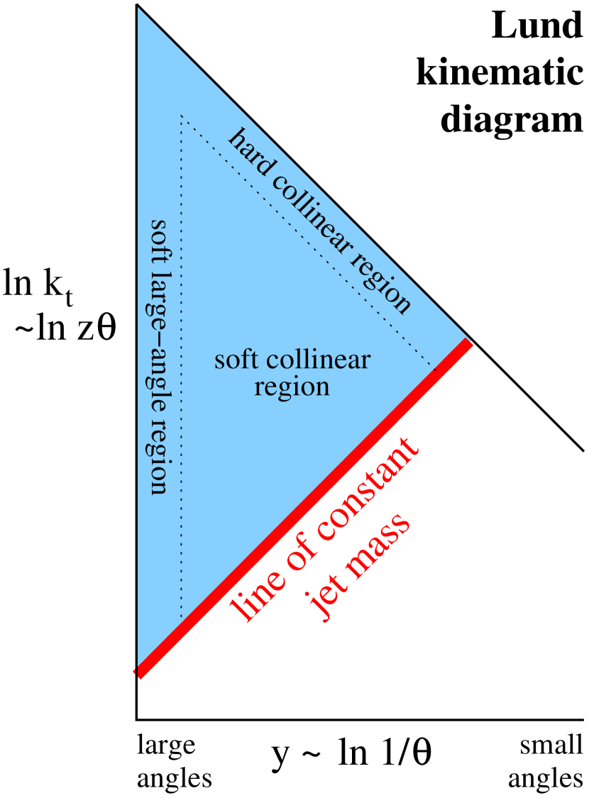
Figure 2: Lund diagrams Andersson:1988gp represent emission kinematics in terms of two variables: vertically, the logarithm of an emission’s transverse momentum $k_{t}$ with respect to the jet axis, and horizontally, the logarithm of the inverse of the emission’s angle $\theta$ with respect to the jet axis, i.e. its rapidity with respect to the jet axis. Here the diagram shows a line of constant jet mass, together with a shaded region corresponding to the part of the kinematic plane where emissions are vetoed, leading to a Sudakov form factor.

To NLL accuracy, i.e. control of terms $\alpha_{s}^{n}L^{n+1}$ and $\alpha_{s}^{n}L^{n}$ in $\ln\Sigma(\rho)$, where $L\equiv\ln\frac{1}{\rho}$, the integrated jet mass distribution is given by

$$\Sigma(\rho)=e^{-D(\rho)}\cdot\frac{e^{-\gamma_{E}D^{\prime}(\rho)}}{\Gamma(1+D^{\prime}(\rho))}\cdot{\cal N}(\rho)\,.$$ (3)

The first factor, which is double logarithmic, accounts for the Sudakov suppression of emissions that would induce a (squared, normalised) jet mass greater than $\rho$. In terms of the “Lund” representation of the kinematic plane Andersson:1988gp , Fig. 2, it accounts for the probability of there being no emissions in the shaded region, with the $\frac{1}{2}\ln^{2}1/\rho$ term in Eq. (2b) for $D(\rho)$ coming from the bulk of the area (soft divergence of $p_{gq}$), while the $-\frac{3}{4}\ln 1/\rho$ term comes from the hard collinear region (finite $z$). The second factor in Eq. (3), defined in terms of $D^{\prime}(\rho)\equiv\partial_{L}D$, encodes the single-logarithmic corrections associated with the fact that the effects of multiple emissions add together to give the jet’s overall mass. These emissions tend to be close to the constant-jet-mass boundary in Fig. 2. The third factor, also single logarithmic, accounts for modifications of the radiation pattern in the jet (non-global logarithms Dasgupta:2001sh ) and boundaries of the jet (clustering logarithms Appleby:2002ke ; Delenda:2006nf ; Kelley:2012kj ) induced by soft radiation near the jet’s edge, i.e. near the left-hand, vertical edge of the shaded region. Had we been working with the anti-$k_{t}$ jet algorithm Cacciari:2008gp , only the non-global logarithms would have been present, which could then be parametrised (in the large-$N_{C}$ limit) as a function ${\cal S}(t)$ of a variable $t(\rho)=\frac{1}{2\pi}\int_{\rho}^{1}\frac{d\rho^{\prime}}{\rho^{\prime}}\alpha_{s}({\rho^{\prime}}^{2}p_{t}^{2}R^{2})$ Dasgupta:2001sh . Note that non-global logarithms are moderately problematic, because their resummation Dasgupta:2001sh ; Dasgupta:2002bw ; Banfi:2002hw ; Hatta:2009nd ; Rubin:2010fc has until very recently always been restricted to the large-$N_{C}$ limit. In effect, non-global logarithms are the main reason why there does not exist a full resummation of the standard jet mass beyond NLL accuracy (for work towards higher accuracy, see Refs. Chien:2012ur ; Jouttenus:2013hs ) and why even the NLL calculations have to neglect some of the terms suppressed by powers of $1/N_{C}^{2}$, as done in Ref. Dasgupta:2012hg .

To visualize the expected behaviour of the jet mass distribution, we can resort to a fixed-coupling approximation, ignoring all but the first factor in Eq. (3), leading to the following differential jet mass distribution

$$\frac{\rho}{\sigma}\frac{d\sigma}{d\rho}\simeq\frac{\alpha_{s}C_{F}}{\pi}\left(\ln\frac{1}{\rho}-\frac{3}{4}\right)e^{-\frac{\alpha_{s}C_{F}}{2\pi}\left(\ln^{2}\frac{1}{\rho}-\frac{3}{2}\ln\frac{1}{\rho}+{\cal O}\left(1\right)\right)}\,.$$ (4)

This shows a characteristic initial growth linear in $\ln\frac{1}{\rho}$ as $\rho$ decreases, cut off by a Sudakov suppression (the exponent) as $\rho$ decreases further. Both of those features are visible in Fig. 1. It is also simple to use Eq. (4) to analytically estimate the position of the peak in $\rho d\sigma/d\rho$. It is given by $L_{\text{peak}}=1/\sqrt{{\bar{\alpha}}_{s}}+{\cal O}\left(1\right)$, where ${\bar{\alpha}}_{s}=\alpha_{s}C_{F}/\pi$ for quark-jets and ${\bar{\alpha}}_{s}=\alpha_{s}C_{A}/\pi$ for gluon-jets . Substituting $\alpha_{s}=0.12$ gives a reasonable degree of agreement with the Monte Carlo peak positions.

4 Trimming

Trimming Krohn:2009th , in the variant that is most widely used today, takes all the particles in a jet of radius $R$ and reclusters them into subjets with a jet definition with radius $R_{\text{sub}}<R$. All resulting subjets that satisfy the condition $p_{t}^{\text{(subjet)}}>z_{\text{cut}}p_{t}^{\text{(jet)}}$ are kept and merged to form the trimmed jet. The other subjets are discarded. While our Monte Carlo results are obtained using the Cambridge/Aachen algorithm (for both the original jet finding and the reclustering), at the accuracy that we shall consider here, our analytical results will hold independently of the jet algorithm used, at least for any member of the generalised-$k_{t}$ family Kt ; KtHH ; Dokshitzer:1997in ; Wobisch:1998wt ; Cacciari:2008gp .

4.1 Leading-order calculation

Let us first consider the situation at leading order. If a gluon is emitted at an angle $\theta>R_{\text{sub}}$ it will be included in the final trimmed jet only if it carries an energy fraction $z>z_{\text{cut}}$. On the other hand, if it is emitted at an angle $\theta<R_{\text{sub}}$, it will be included in the same subjet as the leading parton and will automatically pass the trimming condition. In this case it will contribute to the jet mass independently of its energy fraction $z$.

The above understanding leads to the following integral for the trimmed-mass distribution,

$$\frac{1}{\sigma}\frac{d\sigma}{dm^{2}}^{\text{(trim, LO)}}=\frac{\alpha_{s}C_{F}}{\pi}\int_{0}^{1}dz\,p_{gq}(z)\int\frac{d\theta^{2}}{\theta^{2}}\,\delta\!\left(m^{2}-z(1-z)p_{t}^{2}\theta^{2}\right)\times\\ \times\Big{[}\Theta\left(z-z_{\text{cut}}\right)\Theta\left(1-z-z_{\text{cut}}\right)\Theta(\theta^{2}-R_{\text{sub}}^{2})+\Theta(R_{\text{sub}}^{2}-\theta^{2})\Big{]}\Theta\left(R^{2}-\theta^{2}\right).$$ (5)

It is straightforward to evaluate this for any value of $z_{\text{cut}}$ taggersNLO , but the expressions that we obtain and the subsequent resummation will be much simpler if we assume that $z_{\text{cut}}$ is small (as it usually is in practice), so that we can neglect terms suppressed by powers of $z_{\text{cut}}$. Working furthermore in the approximation $m^{2}\ll p_{t}^{2}R^{2}$, i.e. $\rho\ll 1$, and making use of the fact that $p_{gq}(z)$ is finite for $z\to 1$, we can then discard the middle $\Theta$-function in the first term in square brackets and ignore the $(1-z)$ factors in the $\delta$-function. One may then reorganise the contents of the second line so as to obtain

$$\frac{1}{\sigma}\frac{d\sigma}{dm^{2}}^{\text{(trim, LO)}}=\frac{\alpha_{s}C_{F}}{\pi}\int_{0}^{1}dz\,p_{gq}(z)\int\frac{d\theta^{2}}{\theta^{2}}\,\delta\!\left(m^{2}-zp_{t}^{2}\theta^{2}\right)\times\\ \times\Big{[}\Theta\left(z-z_{\text{cut}}\right)\Theta\left(R^{2}-\theta^{2}\right)+\Theta\left(z_{\text{cut}}-z\right)\Theta(R_{\text{sub}}^{2}-\theta^{2})\Big{]}\,.$$ (6)

Carrying out the integration over $\theta$, and expressing the result in terms of $\rho$ and $r\equiv R_{\text{sub}}/R$ gives

$$\frac{\rho}{\sigma}\frac{d\sigma}{d\rho}^{\text{(trim, LO)}}=\frac{\alpha_{s}C_{F}}{\pi}\int_{0}^{1}dz\,p_{gq}(z)\,\Big{[}\Theta\left(z-z_{\text{cut}}\right)\Theta\left(z-\rho\right)+\Theta\left(z_{\text{cut}}-z\right)\Theta(zr^{2}-\rho)\Big{]}\,.$$ (7)

The remaining $z$ integral is straightforward to evaluate and leads to the following result:

$$\frac{\rho}{\sigma}\frac{d\sigma}{d\rho}^{\text{(trim, LO)}}=\frac{\alpha_{s}C_{F}}{\pi}\left[\Theta\left(\rho-z_{\text{cut}}\right)\ln\frac{1}{\rho}+\Theta\left(z_{\text{cut}}-\rho\right)\ln\frac{1}{z_{\text{cut}}}-\frac{3}{4}\right.+\\ +\left.\Theta\left(z_{\text{cut}}r^{2}-\rho\right)\ln\frac{z_{\text{cut}}r^{2}}{\rho}\right].$$ (8)

For $\rho>z_{\text{cut}}$ this is simply the same as the leading-order jet mass distribution, with a linear growth of the distribution as $\ln 1/\rho$. In the integrated distribution $\Sigma(\rho)$, this corresponds to an $\alpha_{s}L^{2}$ growth, with the two powers of $L$ associated with simultaneous soft and collinear divergences. For $\rho<z_{\text{cut}}$ but $\rho>r^{2}z_{\text{cut}}$ still, the $z_{\text{cut}}$ condition tames the soft divergence: the integrated distribution then goes as $\alpha_{s}L\ln\frac{1}{z_{\text{cut}}}$, dominated by just the collinear divergence. However, because the $z_{\text{cut}}$ condition is applied only to subjets separated by at least $R_{\text{sub}}$ from the main jet, this taming is short-lived: small jet masses with arbitrarily small $z$ values can come from angular regions $\theta<R_{\text{sub}}$. As a result, for $\rho<r^{2}z_{\text{cut}}$, the structure of the result reverts to that for a standard jet mass,

$$\frac{\rho}{\sigma}\frac{d\sigma}{d\rho}^{\text{(trim, LO)}}=\frac{\alpha_{s}C_{F}}{\pi}\left[\ln\frac{r^{2}}{\rho}-\frac{3}{4}\right],\qquad\quad\rho<z_{\text{cut}}r^{2}\,,$$ (9)

albeit with a reduced radius, $R_{\text{sub}}\equiv rR$.

The three situations for the trimmed jet mass can be visualised in Fig. 3 with the help of appropriate Lund kinematic diagrams. The LO integrated cross section $\Sigma(\rho)$ is proportional to the area of the shaded regions, and the differential cross section proportional to the length of the thick (red) line. For $\rho>z_{\text{cut}}$ the integrated cross section corresponds to a triangular region, hence a dependence on $L^{2}$. For $\rho<z_{\text{cut}}$ but $\rho>r^{2}z_{\text{cut}}$, the extra contribution to the integrated cross section comes from a rectangular region, with one side growing with $L$ and the other of fixed length $\simeq\ln 1/z_{\text{cut}}$. This gives an integrated cross section that grows as $L\ln 1/z_{\text{cut}}$, i.e. with only one power of $L$. Finally for $\rho<r^{2}z_{\text{cut}}$ there is once more a triangular region, and so a dependence on $L^{2}$.

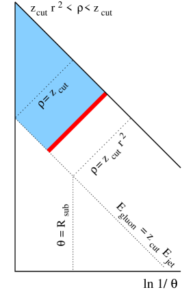
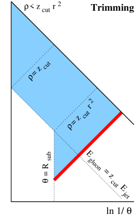
Figure 3: Lund kinematic diagrams for trimming, considering three different possible values of $\rho$. In each case, to obtain the given value of $\rho$, there must be an emission somewhere along the thick (red) line, and there must be no emissions in the shaded region. Emissions in the unshaded regions have no impact on the trimmed jet mass. Dotted lines serve to indicate transition regions in the kinematic plane and their relation to the parameters of the trimmer.

4.2 Resummed calculation

Thanks to the above considerations it is relatively straightforward to obtain an understanding of the all-order trimmed jet-mass distribution. The key result that we use from the extensive literature on event-shape and jet-mass resummations (see e.g. Ref.Catani:1992ua ; Dokshitzer:1998kz ) is that one can effectively use an independent-emission approximation, ignoring subsequent splittings of those emissions, other than in the treatment of the running coupling. This can be understood as a consequence of angular ordering and is sufficient to derive all of Eq. (3) except for the non-global terms. This approach is not necessarily appropriate for all taggers, however it will be suitable for most of the cases in this paper where we give a final resummed answer. The resummation is most easily written for the integrated cross section, involving a sum over an arbitrary number of independent emissions and corresponding virtual corrections. We parametrise each emission in terms of its momentum fraction $z_{i}=E_{i}/E_{\text{jet}}$ and its individual contribution $\rho_{i}=z_{i}\theta_{i}^{2}/R^{2}$ to the squared, normalised jet mass:

$$\Sigma^{\text{(trim)}}(\rho)=\sum_{n=0}^{\infty}\frac{1}{n!}\prod_{i=1}^{n}\int dz_{i}p_{gq}(z_{i})\frac{d\rho_{i}}{\rho_{i}}\frac{\alpha_{s}(\rho_{i}z_{i}p_{t}^{2}R^{2})\,C_{F}}{\pi}\bigg{[}\Theta(\rho-\rho_{i})\,+\\ +\Theta(\rho_{i}-\rho)\Theta(z_{\text{cut}}-z_{i})\Theta(\rho_{i}/r^{2}-z_{i})-1\bigg{]}\Theta(z_{i}-\rho_{i})\,,$$ (10)

There are three terms in the square brackets: the last one corresponds to virtual corrections, while the first two correspond to different regions of real phase-space: the first states that we can sum over any emission whose individual contribution is $\rho_{i}<\rho$; the second states that we can sum over emissions with $\rho_{i}>\rho$, if they are trimmed away, i.e. have $z<z_{\text{cut}}$ and $\theta_{i}>R_{\text{sub}}$ (which is straightforward to express as a condition on $z_{i}<\rho_{i}/r^{2}$). The total contents within the square brackets equal $-1$ in the shaded kinematic regions of Fig. 3 and $0$ elsewhere.

The sum over $n$ in Eq. (10) simply leads to an exponential and we can write the final result as

$$\Sigma^{\text{(trim)}}(\rho)=\exp\Bigg{[}-D(\max(z_{\text{cut}},\rho))-S(z_{\text{cut}},\rho)\Theta(z_{\text{cut}}-\rho)\\ \left.-\Theta(z_{\text{cut}}r^{2}-\rho)\int_{\rho}^{z_{\text{cut}}r^{2}}\frac{d\rho^{\prime}}{\rho^{\prime}}\int^{z_{\text{cut}}}_{\rho^{\prime}/r^{2}}\frac{dz}{z}\frac{C_{F}}{\pi}\,\alpha_{s}(\rho^{\prime}zp_{t}^{2}R^{2})\right]\,.$$ (11)

where $D$ was defined in Eq. (2) and the function $S$ is given by

$$S(a,b) \equiv\frac{C_{F}}{\pi}\int^{a}_{b}\frac{d\rho^{\prime}}{\rho^{\prime}}\int_{z_{\text{cut}}}^{1}dz\,p_{gq}(z)\,\alpha_{s}(\rho^{\prime}z\,p_{t}^{2}R^{2})\,,$$ (12a)

$$\simeq\frac{\alpha_{s}C_{F}}{\pi}\left[\ln\frac{1}{z_{\text{cut}}}-\frac{3}{4}+{\cal O}\left(z_{\text{cut}}\right)\right]\ln\frac{a}{b},\qquad\text{(fixed coupling approx.)}$$ (12b)

and contains only single logarithms, $\alpha_{s}^{n}\ln^{n}\frac{a}{b}$ (treating powers of $\ln\frac{1}{z_{\text{cut}}}$ as finite coefficients). To help better visualise structure of Eq. (11), one may prefer to examine its closed form for fixed coupling:

$$\Sigma^{\text{(trim)}}(\rho)\simeq\exp\left[-\frac{\alpha_{s}C_{F}}{2\pi}\left(-\frac{3}{2}\ln\frac{1}{\rho}\;+\;\Theta(\rho-z_{\text{cut}})\ln^{2}\frac{1}{\rho}+\right.\right.\\ \left.\left.+\Theta(z_{\text{cut}}-\rho)\left(\ln^{2}\frac{1}{z_{\text{cut}}}+2\ln\frac{z_{\text{cut}}}{\rho}\ln\frac{1}{z_{\text{cut}}}\right)+\Theta(z_{\text{cut}}r^{2}-\rho)\ln^{2}\frac{z_{\text{cut}}r^{2}}{\rho}\right)\right]\,.$$ (13)

Eq. (11) resums terms $\alpha_{s}^{n}L^{2n}$ and $\alpha_{s}^{n}L^{2n-1}$ in $\Sigma(\rho)$ (neglecting finite $z_{\text{cut}}$ effects and terms enhanced by powers of $\ln z_{\text{cut}}$). It also resums all terms $\alpha_{s}^{n}L^{n+1}$ in $\ln\Sigma(\rho)$. To obtain what is commonly referred to as NLL accuracy, i.e. all terms $\alpha_{s}^{n}L^{n}$ in $\ln\Sigma(\rho)$, would require a treatment of several additional effects: the two-loop $\beta$-function and cusp anomalous dimension, non-global logarithms involving resummation of terms $\ln(z_{\text{cut}}^{2}r^{2}/\rho)$, related clustering logarithms, and multiple-emission effects on the observable. The clustering logarithms will depend on the jet algorithm used for the trimming, but the rest of the structure will be independent of this (as long as the algorithm belongs to the generalised-$k_{t}$ family). These terms are all relatively straightforward to include, since they follow the structure of the plain jet-mass distribution. However, we leave their study to future work. Analogous results can be also derived for gluon-induced jets. Explicit expressions are collected in appendix A.

4.3 Comparison with Monte Carlo results

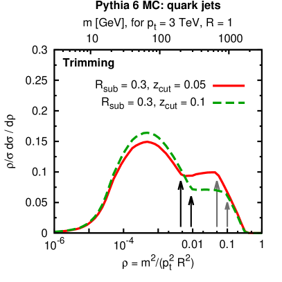
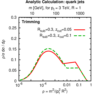
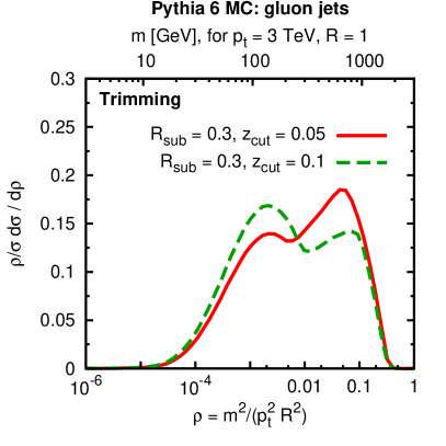
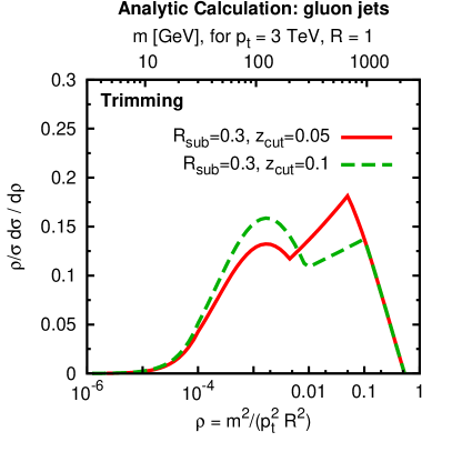
Figure 4: Comparison of Monte Carlo (left panels) and analytic results (right panels) for trimming. The upper panels are for quark jets, the lower panels for gluon jets. Two sets of trimming parameters are illustrated. In the upper left panel, arrows indicate the expected transition points, at $\rho=r^{2}z_{\text{cut}}$ (in black) and $\rho=z_{\text{cut}}$ (in grey), where $r=R_{\text{sub}}/R$. The details of the MC event generation are as for Fig. 1.

One test of Eq. (11) is to compare it to the Monte Carlo results. We do this in Fig. 4 where the left-hand plots show the trimmed-mass distribution as obtained with Monte Carlo simulation and the right-hand plots shows the corresponding analytical results. The upper row is for quark-initiated jets, while the lower one is for gluon-initiated jets. Two sets of trimming parameters are shown, to help visualize the dependence on them.

The three regions of $\rho$ are clearly distinguishable in each plot, with a close correspondence of the Monte Carlo and analytic shapes and transition points, as well as their dependence on the trimming parameters. Specifically, in the case of quark jets, for $\rho>z_{\text{cut}}$, one sees a linear rise with $\ln 1/\rho$. For $\rho<z_{\text{cut}}$, down to $\rho=r^{2}z_{\text{cut}}$ there is an approximate plateau, whose height increases for smaller $z_{\text{cut}}$, as expected from the $\ln 1/z_{\text{cut}}$ term for this region in the LO formula, Eq. (8). For $\rho<r^{2}z_{\text{cut}}$, the linear rise starts again, but is quickly suppressed by a Sudakov form factor, giving the usual jet-mass type peak. The case of gluon-initiated jets is similar, although the single-logarithmic region is not flat, because of the specific choices of $z_{\text{cut}}$.

Insofar as $z_{\text{cut}}$ and $R_{\text{sub}}$ are not too small, the peak position is essentially given by the peak position for the mass of a jet of size $R_{\text{sub}}$ rather than $R$,

$$L_{\text{peak}}^{\text{trim}}=\frac{1}{\sqrt{{\bar{\alpha}}_{s}}}-2\ln r+{\cal O}\left(1\right)\,.$$ (14)

i.e. at a $\rho$ value that is a factor $r^{2}$ smaller than for the plain jet mass. This is consistent with what is observed comparing the Monte Carlo results for the plain and trimmed jet masses. A final comment is that while the peak position is independent of $z_{\text{cut}}$, its height is not: the smaller the value of $z_{\text{cut}}$, the greater the Sudakov suppression associated with vetoing emissions in the range $z_{\text{cut}}r^{2}<\rho<z_{\text{cut}}$, and so the smaller the peak height, again in accord with the Monte Carlo results.

5 Pruning

Pruning Ellis:2009me ; Ellis:2009su takes an initial jet, and from its mass deduces a pruning radius $R_{\text{prune}}=R_{\text{fact}}\cdot\frac{2m}{p_{t}}$, where $R_{\text{fact}}$ is a parameter of the tagger. It then reclusters the jet and for every clustering step, involving objects $a$ and $b$, it checks whether $\Delta_{ab}>R_{\text{prune}}$ and $\min(p_{ta},p_{tb})<z_{\text{cut}}p_{t,(a+b)}$, where $z_{\text{cut}}$ is a second parameter of the tagger. If so, then the softer of the $a$ and $b$ is discarded. Otherwise $a$ and $b$ are recombined as usual. Clustering then proceeds with the remaining objects, applying the pruning check at each stage.

In analysing pruning, we will take $R_{\text{fact}}=\frac{1}{2}$, i.e. its default suggested value Ellis:2009su . In analogy with our approach for trimming, we will work in the limit of small $z_{\text{cut}}$ (but $\ln z_{\text{cut}}$ not too large). We will assume that the reclustering is performed with the Cambridge/Aachen algorithm, the most common choice, and that adopted by CMS CMS-substructure-studies . ATLAS Aad:2013gja have instead performed the reclustering with the $k_{t}$ algorithm Kt ; KtHH ). Similar methods could be used to study that case, but we leave such an investigation to future work.

5.1 Leading-order calculation

At leading order, i.e. a jet involving a single $1\to 2$ splitting, $R_{\text{prune}}=\frac{m}{p_{t}}=\Delta_{ab}\sqrt{z(1-z)}$, which guarantees that $\Delta_{ab}$ is always larger than $R_{\text{prune}}$. To establish the pruned jet mass, one then needs to examine the second part of the pruning condition: if $\min(z,1-z)>z_{\text{cut}}$ then the clustering is accepted and the pruned jet has a finite mass. Otherwise the pruned jet mass is zero. This pattern is true independently of the angle between the two prongs. This leads to the following result for the mass distribution:

$$\frac{1}{\sigma}\frac{d\sigma}{dm^{2}}^{\text{(prune, LO)}} =\frac{\alpha_{s}C_{F}}{\pi}\int dz\,p_{gq}(z)\,\frac{d\theta^{2}}{\theta^{2}}\,\delta\!\left(m^{2}-z(1-z)p_{t}^{2}\theta^{2}\right)\times$$ (15)

$$\qquad\qquad\qquad\times\Theta\left(z-z_{\text{cut}}\right)\Theta\left((1-z)-z_{\text{cut}}\right)\Theta\left(R^{2}-\theta^{2}\right),$$

$$=\frac{\alpha_{s}C_{F}}{\pi}\int dz\,p_{gq}(z)\,\frac{1}{m^{2}}\,\Theta\left(z-z_{\text{cut}}\right)\Theta\left(z-\frac{m^{2}}{p_{t}^{2}R^{2}}\right),$$ (16)

where to obtain the last line we have made use of the fact that $z_{\text{cut}}$ is small and that the integral is dominated by the region $z\ll 1$. The final $z$-integration is straightforward to perform and gives

$$\frac{\rho}{\sigma}\frac{d\sigma}{d\rho}^{\text{(prune, LO)}}=\frac{\alpha_{s}C_{F}}{\pi}\left[\Theta(\rho-z_{\text{cut}})\ln\frac{1}{\rho}+\Theta(z_{\text{cut}}-\rho)\ln\frac{1}{z_{\text{cut}}}-\frac{3}{4}\right].$$ (17)

This has the structure of a rise linear in $\ln\rho$ for $\rho$ down to $z_{\text{cut}}$, and then it is constant below. For small $\rho$, the corresponding integrated cross section has the remarkable property that it contains no double-logarithmic terms, i.e. no $\alpha_{s}L^{2}$ contribution. This is, in a certain sense, what pruning was, in our understanding, intended to achieve: the double-log contribution comes from the region of arbitrarily soft gluon emission, and pruning removes such soft emissions.

5.2 3-particle configurations: Y-pruning and I-pruning

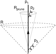
Figure 5: Configuration that illustrates generation of double logs in pruning at ${\cal O}\left(\alpha_{s}^{2}\right)$. Soft gluon $p_{3}$ dominates the jet mass, thus determining the pruning radius. However, because of $p_{3}$’s softness, it is then pruned away, leaving only the central core of the jet, which has a usual double-logarithmic type mass distribution.

When we consider 3-particle configurations the behaviour of pruning develops a certain degree of complexity. Fig. 5 illustrates the type of configuration that is responsible: there is a soft parton ($p_{3}$) that dominates the total jet mass and so sets the pruning radius, but it does not pass the pruning $z_{\text{cut}}$ threshold, meaning that it does not contribute to the pruned mass; meanwhile there is another parton ($p_{2}$), within the pruning radius, that contributes to the pruned jet mass independently of how soft it is. We call this “I-pruning”, because at the angular scale $R_{\text{prune}}$, the final pruned jet consists of a single prong. It is to be contrasted with the type of configuration that contributed to the leading order result Eq. (17), for which at an angular scale $R_{\text{prune}}$, the pruned jet always consisted of two prongs. That we call “Y-pruning”.

Let us work through I-pruning quantitatively. For gluon $3$ to be discarded by pruning it must have $z_{3}<z_{\text{cut}}\ll 1$, i.e. it must be soft. Then the pruning radius is given by $R_{\text{prune}}^{2}=z_{3}\theta_{3}^{2}$ and for $p_{2}$ to be within the pruning core we have $\theta_{2}<R_{\text{prune}}$. This implies $\theta_{2}\ll\theta_{3}$, which allows us to treat $p_{2}$ and $p_{3}$ as being emitted independently (i.e. due to angular ordering) and also means that the C/A algorithm will first cluster $1+2$ and then $(1+2)+3$. The leading-logarithmic contribution that one then obtains at ${\cal O}\left(\alpha_{s}^{2}\right)$ is

$$\frac{\rho}{\sigma}\frac{d\sigma^{\text{(I-prune, NLO)}}}{d\rho} \simeq\left(\frac{C_{F}\alpha_{s}}{\pi}\right)^{2}\int_{0}^{z_{\text{cut}}}\frac{dz_{3}}{z_{3}}\int^{R^{2}}\frac{d\theta_{3}^{2}}{\theta_{3}^{2}}\int_{0}^{1}\frac{dz_{2}}{z_{2}}\int_{0}^{z_{3}\theta_{3}^{2}}\frac{d\theta_{2}^{2}}{\theta_{2}^{2}}\;\rho\,\delta\left(\rho-z_{2}\frac{\theta_{2}^{2}}{R^{2}}\right)$$ (18a)

$$=\left(\frac{C_{F}\alpha_{s}}{\pi}\right)^{2}\frac{1}{6}\ln^{3}\frac{z_{\text{cut}}}{\rho}+{\cal O}\left(\alpha_{s}^{2}\ln^{2}\frac{1}{\rho}\right),\qquad\text{(valid for $\rho<z_{\text{cut}}$)},$$ (18b)

where we have directly taken the soft limits of the relevant splitting functions.

The $\ln^{3}\rho$ contribution that one observes here in the differential distribution corresponds to a double logarithmic ($\alpha_{s}^{2}\ln^{4}\rho$) behaviour of the integrated cross-section, i.e. it has as many logs as the raw jet mass, with both soft and collinear origins. This term is the first of a whole tower of terms $\alpha_{s}^{n}\ln^{2n}\rho$, all associated with configurations where the emission(s) that set the total jet mass are discarded during pruning, leaving just the mass of the core of the jet (at angles smaller than $R_{\text{prune}}$).

In general, substructure taggers aim to eliminate contributions from soft emission. What we see here is that this is not entirely the case for pruning. However, in an experimental analysis, it is easy to diagnose whether configurations such as that in Fig. 5 have arisen. Accordingly, we introduce explicit operative definitions for I-pruning and its converse, Y-pruning:

• Y-pruning: if at any stage during the sequential recombination there was a clustering that satisfied the $\Delta_{ab}>R_{\text{prune}}$ condition and the requirement $\frac{\min(p_{t,a},p_{t,b})}{p_{t,(a+b)}}>z_{\text{cut}}$, the jet is deemed to pass the Y-pruning (i.e. two-prong) requirement. The jet mass was dominated by (semi)-hard radiation and it is likely that the pruning radius was set appropriately for that radiation.

• I-pruning: if during the sequential recombination there was never a clustering satisfying the $\Delta_{ab}>R_{\text{prune}}$ condition and the requirement $\frac{\min(p_{t,a},p_{t,b})}{p_{t,(a+b)}}>z_{\text{cut}}$, the jet is deemed to belong to the I- (i.e. one-prong) pruned class. Typically, for this class of jets, the jet mass was dominated by soft emissions, leading to a pruning radius that had no relation to any hard substructure potentially present in the jet.

According to our first definition of grooming and tagging in section 2, generic pruning is a grooming procedure: given an initial jet, there is always a corresponding pruned jet, though often with a different mass. In contrast, according to that same definition, Y-pruning is a tagger: i.e. given some initial jet, there will not always be a corresponding Y-pruned jet. In the Monte Carlo results that we will discuss below in section 5.4, for our default choice of pruning parameters, Y-pruning tags about $40\%$ of QCD jets.

Let us examine the $\alpha_{s}^{2}$ contribution for Y-pruning. Physically, the key addition relative to the LO result (for which we exclusively have Y-pruning) is the requirement that there should have been no radiation $p_{3}$ that would set a pruning radius larger than $\theta_{2}$, i.e. no radiation with $\rho_{3}\equiv z_{3}\theta_{3}^{2}>\theta_{2}^{2}$. Insofar as we neglect logarithms of $z_{\text{cut}}$, we can replace this with the condition $\rho_{3}>\rho_{2}\equiv\rho$, resulting in a structure up to $\alpha_{s}^{2}$ of

$$\frac{\rho}{\sigma}\frac{d\sigma^{\text{(Y-prune, NLO)}}}{d\rho}\simeq\frac{\alpha_{s}C_{F}}{\pi}\left(\ln\frac{1}{z_{\text{cut}}}-\frac{3}{4}\right)\times\left[1-\frac{\alpha_{s}C_{F}}{2\pi}\ln^{2}\frac{1}{\rho}\right]\,,\qquad\rho<z_{\text{cut}}^{2}\,.$$ (19)

where the round bracket comes (as at LO), from the integral over allowed $z_{2}$ values, and we have used a double-logarithmic approximation for the contents of the square brackets. Translating to the integrated distribution, Eq. (19) implies the presence of a term of the form $\alpha_{s}^{2}\ln^{3}1/\rho$, i.e. with one logarithm fewer than the I-pruning contribution. As we shall see below, this difference will be related to highly distinct resummation structures for the two types of contribution.

5.3 Resummed results

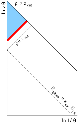
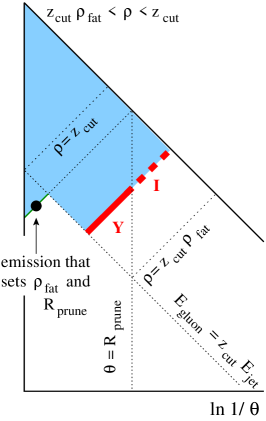
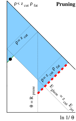
Figure 6: Lund kinematic diagrams for pruning, considering three different possible values of $\rho$. In each case, to obtain the given value of $\rho$, there must be an emission somewhere along the thick (red) line, and there must be no emissions in the shaded region. The solid part of the thick line corresponds to Y-pruning, while the dashed part gives I-pruning. Emissions in the unshaded regions have no impact on the pruned jet mass. The behaviour of the pruner can be affected by the presence of an emission that dominates $\rho_{\text{fat}}$ (and so sets the pruning radius), but is discarded because it is below the pruning energy cut. The dotted line that shows the pruning energy cut is parametrised in terms of the jet energy; this is a simplification, insofar as pruning uses the local subjet to provide its reference energy.

To understand how to resum the pruned jet mass, for both the Y and I components, it is useful to refer to Fig. 6. The left-most figure corresponds to the the region $\rho>z_{\text{cut}}$ and is essentially identical to the plain jet mass (as for trimming in this region). In this region we only have Y-pruning.

The middle and right-hand plots illustrate two of the main configurations that are relevant when $\rho<z_{\text{cut}}$. Both show an emission (small black disk) that dominates the total jet mass ($\rho_{\text{fat}}$) and so sets the pruning radius

$$R_{\text{prune}}^{2}=\rho_{\text{fat}}\,R^{2}\,.$$ (20)

It will always be at an angle larger than $R_{\text{prune}}$, and for the discussion here it will be interesting to consider the cases where it has a momentum fraction $z_{\text{fat}}<z_{\text{cut}}$, so that it is pruned away. We then need to consider a second emission, somewhere along the thick (red) solid and dashed lines, with momentum fraction $z$ and angle $\theta$, that sets the final pruned mass $\rho$. The two possible situations are:

Y-pruning: $$\quad\theta>R_{\text{prune}},\;z>z_{\text{cut}}\quad\longrightarrow\quad z_{\text{cut}}<z<\frac{\rho}{\rho_{\text{fat}}}\,,$$ (21a)

I-pruning: $$\quad\theta<R_{\text{prune}},\phantom{\;z>z_{\text{cut}}}\quad\longrightarrow\quad z>\frac{\rho}{\rho_{\text{fat}}}\,,$$ (21b)

where the conditions on $z$ have been derived by combining the relation $\theta^{2}=\rho R^{2}/z$ with Eq. (20).

In the middle panel of Fig. 6, the Y-pruning region is represented by a thick (red) solid line, while the I-pruning region is represented by a thick (red) dashed line.

In the rightmost panel, with $\rho/\rho_{\text{fat}}<z_{\text{cut}}$, there can be no Y-pruning, because emissions with $\theta>R_{\text{prune}}$ necessarily have $z<\rho/\rho_{\text{fat}}<z_{\text{cut}}$. There is then only I-pruning, and because there is no direct constraint on the momentum fraction of emissions with $\theta<R_{\text{prune}}$, any $z>\rho/\rho_{\text{fat}}$ contributes to the I-pruning, even if $z<z_{\text{cut}}$. Given that $\rho_{\text{fat}}<z_{\text{cut}}$, I-pruning with $z<z_{\text{cut}}$ starts to appear only for $\rho<z_{\text{cut}}^{2}$.

To determine the distributions for Y- and I-pruning, we will work, as for trimming, in an independent emission picture. However, for brevity, we will not explicitly write the independent emissions here, but instead make use of the result that when one forbids emissions (i.e. the shaded regions of Fig. 6), one simply includes a factor corresponding to the exponential of (minus) the integral of the coupling times the splitting function over the forbidden region.

5.3.1 Y-pruning

For Y-pruning, one way of writing the result is as an integral over the momentum fraction $z$ of the emission that gives the final pruned mass. For a given $z$ to contribute it must obviously satisfy $z>z_{\text{cut}}$. In addition the fat jet mass must be smaller than $\rho/z$. From the considerations of the previous section, this then gives us, for $\rho<z_{\text{cut}}$,

$$\frac{\rho}{\sigma}\frac{d\sigma^{\text{(Y-prune)}}}{d\rho}=\int_{z_{\text{cut}}}^{1}dz\;p_{gq}(z)\;e^{-D\left(\min(z_{\text{cut}},\frac{\rho}{z})\right)-S\left(\min(z_{\text{cut}},\frac{\rho}{z}),\rho\right)}\frac{\alpha_{s}(\rho z\,p_{t}^{2}R^{2})\,C_{F}}{\pi}\,.$$ (22)

The $D\left(\min(z_{\text{cut}},\frac{\rho}{z})\right)$ terms accounts for the suppression of all emissions that would produce a $\rho_{\text{fat}}>\rho/z$ (or $\rho_{\text{fat}}>z_{\text{cut}}$). The term $S\left(\min(z_{\text{cut}},\frac{\rho}{z}),\rho\right)$ accounts for the further required suppression of emissions with $z>z_{\text{cut}}$ contributing a mass between $\rho/z$ and $\rho$.

Another, equivalent way of writing the result makes the $\rho_{\text{fat}}$ integral more explicit:

$$\frac{\rho}{\sigma}\frac{d\sigma^{\text{(Y-prune)}}}{d\rho}=e^{-D\left(\rho\right)}\int_{z_{\text{cut}}}^{1}dz\;p_{gq}(z)\frac{\alpha_{s}(\rho z\,p_{t}^{2}R^{2})\,C_{F}}{\pi}\;+\\ +\int_{\rho}^{\min(z_{\text{cut}},\rho/z_{\text{cut}})}\frac{d\rho_{\text{fat}}}{\rho_{\text{fat}}}\left(e^{-D(\rho_{\text{fat}})}\int_{\rho_{\text{fat}}}^{z_{\text{cut}}}\frac{dz^{\prime}}{z^{\prime}}\frac{\alpha_{s}(\rho_{\text{fat}}z^{\prime}\,p_{t}^{2}R^{2})\,C_{F}}{\pi}\right)\times\\ \times e^{-S\left(\rho_{\text{fat}},\rho\right)}\int_{z_{\text{cut}}}^{\rho/\rho_{\text{fat}}}dz\;p_{gq}(z)\frac{\alpha_{s}(\rho z\,p_{t}^{2}R^{2})\,C_{F}}{\pi}\,.$$ (23)

The term on the first line corresponds to configurations in which the emission that dominates the pruned mass also dominates the overall fat-jet mass. The term on the second and third lines corresponds to situations where there is an explicit emission with momentum fraction $z^{\prime}<z_{\text{cut}}$ that gets pruned away. It sets a fat-jet mass substantially larger than the final pruned mass, $\rho_{\text{fat}}\gg\rho$, while the emission that dominates the pruned mass still has $\theta>R_{\text{prune}}$.

The above two expressions should capture terms $\alpha_{s}^{n}L^{2n-1}$ and $\alpha_{s}^{n}L^{2n-2}$ in $\Sigma^{\text{(Y-prune)}}(\rho)$. It is less straightforward to discuss the accuracy for $\ln\Sigma^{\text{(Y-prune)}}(\rho)$: this is because unlike the cases of plain jet mass and trimming, pruning does not lead to a simple exponentiated structure. Analogous results for gluon-initiated jets are given in appendix A.3.

To help understand the structure of Eqs. (22) and (23), it is useful to evaluate them in a fixed-coupling approximation, neglecting terms $\sim\alpha_{s}\ln^{2}z_{\text{cut}}$, which for $\rho<z_{\text{cut}}^{2}$ yields

$$\frac{\rho}{\sigma}\frac{d\sigma^{\text{(Y-prune)}}}{d\rho} \simeq e^{-D(\rho)}\left[\left(e^{\frac{\alpha_{s}C_{F}}{\pi}\ln\frac{1}{z_{\text{cut}}}\ln\frac{1}{\rho}}-1\right)\frac{1}{\ln\frac{1}{\rho}}-\frac{3}{4}\frac{\alpha_{s}C_{F}}{\pi}\right]$$ (24a)

$$\simeq e^{-D(\rho)}\,\frac{\alpha_{s}C_{F}}{\pi}\left[\ln\frac{1}{z_{\text{cut}}}-\frac{3}{4}\right]\,,\qquad\alpha_{s}\ln\frac{1}{z_{\text{cut}}}\ln\frac{1}{\rho}\ll 1\,,$$ (24b)

where the second line provides a further simplification for situations where $\rho$ is not too small and illustrates the consistency with Eq. (19).

5.3.2 I-pruning

The resummed result for I-pruning reads for $\rho<z_{\text{cut}}$

$$\frac{\rho}{\sigma}\frac{d\sigma^{\text{(I-prune)}}}{d\rho}=\int_{\rho}^{z_{\text{cut}}}\frac{d\rho_{\text{fat}}}{\rho_{\text{fat}}}\left(e^{-D(\rho_{\text{fat}})}\int_{\rho_{\text{fat}}}^{z_{\text{cut}}}\frac{dz^{\prime}}{z^{\prime}}\frac{\alpha_{s}(\rho_{\text{fat}}z^{\prime}\,p_{t}^{2}R^{2})\,C_{F}}{\pi}\right)\times\\ \times e^{-S\left(\rho_{\text{fat}},\rho\right)}\int_{\rho/\rho_{\text{fat}}}^{1}dz\;p_{gq}(z)\frac{\alpha_{s}(\rho z\,p_{t}^{2}R^{2})\,C_{F}}{\pi}\left[\Theta\left(\frac{\rho}{\rho_{\text{fat}}}-z_{\text{cut}}\right)+\right.\\ \left.+\Theta\left(z_{\text{cut}}-\frac{\rho}{\rho_{\text{fat}}}\right)\exp\left(-\int_{\rho}^{z_{\text{cut}}\rho_{\text{fat}}}\frac{d\rho^{\prime}}{\rho^{\prime}}\int_{\rho^{\prime}/\rho_{\text{fat}}}^{z_{\text{cut}}}\frac{dz^{\prime}}{z^{\prime}}\frac{C_{F}}{\pi}\alpha_{s}(\rho^{\prime}z^{\prime}p_{t}^{2}R^{2})\right)\right]\,.$$ (25)

In order to have I-pruning, there must be an emission that sets the fat-jet mass and pruning radius such that that first emission gets pruned away and a second emission falls within the pruning radius. The first line of Eq. (25) gives the distribution for the fat-jet mass, assuming that the corresponding emission has $z<z_{\text{cut}}$, i.e. gets pruned away. The second line includes a Sudakov suppression $e^{-S(\rho_{\text{fat}},\rho)}$ for forbidding emissions with $z>z_{\text{cut}}$ between the scales of $\rho_{\text{fat}}$ and $\rho$, and also includes an integral over the allowed $z$ values for emissions that fall within the pruning radius. This multiplies a square bracket containing two terms: the first corresponds to the middle diagram of Fig. 6, while the second corresponds to the right-hand diagram, and accounts for the required additional Sudakov suppression of emissions with $z<z_{\text{cut}}$ and $\theta<R_{\text{prune}}$. In this factor, we have directly replaced $dz\,p_{gq}(z)$ with $dz/z$, neglecting corrections suppressed by powers of $z_{\text{cut}}$.

Eq. (25) should account for terms $\alpha_{s}^{n}L^{2n}$ and $\alpha_{s}^{n}L^{2n-1}$ in $\Sigma^{\text{(I-prune)}}$, i.e. the first two towers of logarithms. Note that overall we have one power of $L$ more than for Y-pruning. As for the case of Y-pruning, it is less straightforward to discuss the accuracy for $\ln\Sigma^{\text{(I-prune)}}$. Analogous results for gluon-initiated jets are given in appendix A.3. A calculation beyond the small-$z_{\text{cut}}$ limit reveals that there are flavour-changing contributions that mix quark-initiated and gluon-initiated jets. They give rise to terms $\sim z_{\text{cut}}\alpha_{s}^{n}L^{2n-1}$ taggersNLO , and they are neglected here because they vanish as $z_{\text{cut}}\to 0$.

The structure of Eq. (25) is relatively complicated. Accordingly, to gain some insight into it we will make a double logarithmic approximation, considering just terms $\alpha_{s}^{n}L^{2n}$ in $\Sigma^{\text{(I-prune)}}(\rho)$. Within this approximation we can replace $p_{gq}(z)$ with $1/z$, assume $z_{\text{cut}}$ to be of order $1$ and take $\alpha_{s}$ fixed. This then gives

$$\frac{\rho}{\sigma}\frac{d\sigma^{\text{(I-prune)}}}{d\rho}\simeq\left(\frac{\alpha_{s}C_{F}}{\pi}\right)^{2}\int_{\rho}^{1}\frac{d\rho_{\text{fat}}}{\rho_{\text{fat}}}\ln\rho_{\text{fat}}e^{-\frac{1}{2}\frac{\alpha_{s}C_{F}}{\pi}\ln^{2}\frac{1}{\rho_{\text{fat}}}}\,\ln\frac{\rho}{\rho_{\text{fat}}}e^{-\frac{1}{2}\frac{\alpha_{s}C_{F}}{\pi}\ln^{2}\frac{\rho_{\text{fat}}}{\rho}}\,,$$ (26)

which integrates to

$$\frac{\rho}{\sigma}\frac{d\sigma^{\text{(I-prune)}}}{d\rho}\simeq\frac{{\bar{\alpha}}_{s}L}{2}e^{-\frac{1}{2}{\bar{\alpha}}_{s}L^{2}}+\frac{\sqrt{{\bar{\alpha}}_{s}\pi}}{4}e^{-\frac{1}{4}{\bar{\alpha}}_{s}L^{2}}(-2+{\bar{\alpha}}_{s}L^{2})\,\mathrm{Erf}\left(\frac{\sqrt{{\bar{\alpha}}_{s}}L}{2}\right)\,.$$ (27)

It is straightforward to verify that this has no $\alpha_{s}$ term and is equivalent to Eq. (18a) at order $\alpha_{s}^{2}$. The structure involving the factor $L^{2}e^{-\frac{1}{4}{\bar{\alpha}}_{s}L^{2}}$ can be seen to arise from the point where the integrand in Eq. (26) is maximal. Insofar as it is legitimate to consider just this structure, one might expect the I-pruned mass distribution to have a maximum situated near $L=2/\sqrt{{\bar{\alpha}}_{s}}$. Using the full form of Eq. (27), the maximum is at $L\simeq 2.284/\sqrt{{\bar{\alpha}}_{s}}$, which is to be compared to the maximum of the plain jet-mass distribution, situated at $L=1/\sqrt{{\bar{\alpha}}_{s}}$. We will return to these observations when we discuss comparisons with Monte Carlo below.

5.3.3 Sum of Y and I components

Finally let us add together Y- and I-pruning in the region $z_{\text{cut}}^{2}<\rho<z_{\text{cut}}$, working in a fixed-coupling approximation for simplicity. In this region, the upper limit of the $\rho_{\text{fat}}$ integrals in Eqs. (23) and (25) becomes $z_{\text{cut}}$. In the square brackets of Eq. (25), it is the first of the $\Theta$-functions that is relevant (because we have $\rho_{\text{fat}}<z_{\text{cut}}$ and $\rho>z_{\text{cut}}^{2}$). The $z$ integrals in Eqs. (23) and (25) are associated with the same prefactors and $\rho_{\text{fat}}$ integration, and have complementary limits in $z$, $z_{\text{cut}}<z<\rho/\rho_{\text{fat}}$ and $\rho/\rho_{\text{fat}}<z<1$ respectively and so add together to give an integral over $z$ from $z_{\text{cut}}$ to $1$. We can therefore write the sum as

$$\frac{\rho}{\sigma}\frac{d\sigma^{\text{(prune)}}}{d\rho}=\int_{z_{\text{cut}}}^{1}dz\;p_{gq}(z){\bar{\alpha}}_{s}\left(e^{-D\left(\rho\right)}+\int_{\rho}^{z_{\text{cut}}}d\rho_{\text{fat}}\left(e^{-D(\rho_{\text{fat}})-S\left(\rho_{\text{fat}},\rho\right)}\int_{\rho_{\text{fat}}}^{z_{\text{cut}}}\frac{dz^{\prime}}{z^{\prime}}{\bar{\alpha}}_{s}\right)\right)\,.$$ (28)

Using a fixed-coupling approximation for simplicity, and making use of the fact that

$$D(\rho)=D(z_{\text{cut}})+S(z_{\text{cut}},\rho)+\frac{{\bar{\alpha}}_{s}}{2}\ln^{2}\frac{z_{\text{cut}}}{\rho}+{\cal O}\left({\bar{\alpha}}_{s}z_{\text{cut}}\right)\,,$$ (29)

we then obtain the simple result

$$\frac{\rho}{\sigma}\frac{d\sigma^{\text{(prune)}}}{d\rho}=e^{-D(z_{\text{cut}})+S(z_{\text{cut}},\rho)}{\bar{\alpha}}_{s}\left(\ln\frac{1}{z_{\text{cut}}}-\frac{3}{4}\right)\,,\qquad z_{\text{cut}}^{2}<\rho<z_{\text{cut}}\,,$$ (30)

which corresponds to the following integrated cross section:

$$\Sigma^{\text{(prune)}}(\rho)=e^{-D(z_{\text{cut}})+S(z_{\text{cut}},\rho)}\,,\qquad z_{\text{cut}}^{2}<\rho<z_{\text{cut}}\,.$$ (31)

This second form holds also with running coupling effects included.

Several comments can be made about Eq. (31). Relative to the middle panel of Fig. 6, the key point is that for $z_{\text{cut}}^{2}<\rho<z_{\text{cut}}$, the presence or not of a distinct “fat-jet” emission (one with $z^{\prime}<z_{\text{cut}}$) only modifies the separation between I and Y-pruning, but not their sum. As a result, $-\ln\Sigma(\rho)$ is effectively just the integral of the leading order distribution, Eq. (17). This is the pattern that is seen also for trimming and the plain jet mass (at NLL accuracy in $\Sigma$), but with the difference that in the case of pruning the pattern breaks down for $\rho<z_{\text{cut}}^{2}$, whereas for trimming and plain jet mass it holds for all $\rho$ values.

Another point of interest is that Eq. (31) is identical to the result for trimming, Eq. (13), in the corresponding region $r^{2}z_{\text{cut}}<\rho<z_{\text{cut}}$. Trimming and pruning are also identical, at our accuracy, for $\rho>z_{\text{cut}}$. We will return to this point later when we discuss the comparisons between taggers in section 8.1.

Finally, as in the case of trimming, to go beyond the accuracy aimed for in this paper for pruning would require the treatment of several additional effects: non-global logarithms and related clustering logarithms, multiple-emission effects on the observable and the two-loop cusp anomalous dimension.

Non-global logarithms enter in a number of ways: in particular, from the boundary at $\theta\sim R$, they affect the fat-jet mass, and through it the distribution of the pruning radius. This has implications for both the Y and I components starting, in the small-$z_{\text{cut}}$ limit, from order $\alpha_{s}^{3}$. Moreover, at finite $z_{\text{cut}}$, I-pruning receives non-global contributions already at order $\alpha_{s}^{2}$ taggersNLO . We leave a full resummation of pruning to single-logarithmic accuracy to future work.

5.4 Comparison with Monte Carlo results

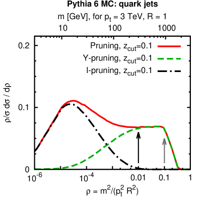
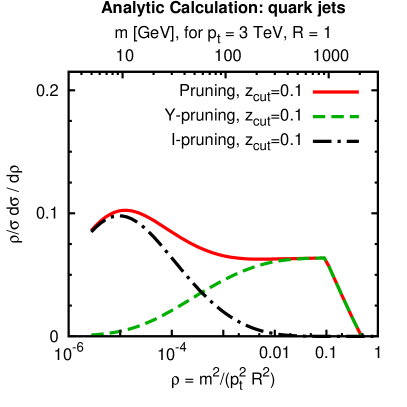
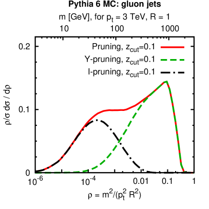
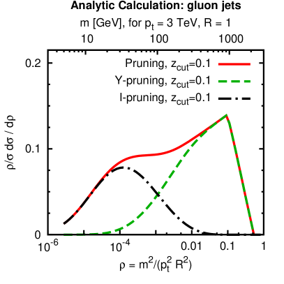
Figure 7: Comparison of Monte Carlo (left panels) and analytic results (right panels) for pruning. The upper panels are for quark jets, the lower panels for gluon jets. The plots show full pruning as well as its breakdown into Y and I components. In the upper left panel, arrows indicate the expected transition points, at $\rho=z_{\text{cut}}^{2}$ (in black) and $\rho=z_{\text{cut}}$ (in grey). The details of the MC event generation are as for Fig. 1.

Figure 7 shows predictions for the pruned mass distribution from Pythia in the left-hand panels and from our analytical calculation in the right-hand panels. Upper and lower rows correspond to quark jets and gluon jets respectively. As was the case with trimming, the agreement between the MC and analytical results is reasonable. The expected transition points at $\rho=z_{\text{cut}}$ and $z_{\text{cut}}^{2}$ are labelled with arrows in the upper MC plot. Above $\rho=z_{\text{cut}}$ we see a similar behaviour as for the plain jet mass. For $z_{\text{cut}}^{2}<\rho<z_{\text{cut}}$, we see a flat region in the quark case, akin to the leading-order result, however in the gluon case that flatness is strongly modified by higher orders (the exact impact of these higher orders depends strongly on $z_{\text{cut}}$). The transition at $\rho=z_{\text{cut}}^{2}$ is much smoother than that at $z_{\text{cut}}$. Recall that the transition occurs because phase space opens for emissions with $z<z_{\text{cut}}$ to dominate the pruned jet mass. As one can verify analytically, that phase space initially opens up slowly (cf. also Fig. 6) and the most singular contribution for pruning (Y+I components) goes as $\alpha_{s}^{2}\ln^{3}z_{\text{cut}}^{2}/\rho$. The transition is therefore gradual.

Going substantially below $\rho=z_{\text{cut}}^{2}$, for quark jets, one sees a clear peak in total pruning, which results from the I component. In the gluon case, while that peak is similarly visible in the I component, in the sum with Y-pruning it manifests itself as a shoulder, because the peak occurs in a region where the Y-pruning component is not entirely suppressed. As before, this precise picture holds for our specific choice of $z_{\text{cut}}$.

The position of the peak for the I component, in the case of quark-initiated jets, is in reasonable agreement with the one determined by the fixed-coupling approximation, Eq. (27), though the agreement is poorer for gluon jets: for a reliable quantitative treatment of the peak region it is important to include subleading terms.

6 Mass Drop Tagger

The mass-drop tagger Butterworth:2008iy was designed to be used with jets found by the Cambridge/Aachen algorithm Dokshitzer:1997in ; Wobisch:1998wt . It involves two parameters $y_{\text{cut}}$ and $\mu$ and, for an initial jet labelled $j$, proceeds as follows:

1. Break the jet $j$ into two subjets by undoing its last stage of clustering. Label the two subjets $j_{1},j_{2}$ such that $m_{j_{1}}>m_{j_{2}}$.

2. If there was a significant mass drop, $m_{j_{1}}<\mu m_{j}$, and the splitting is not too asymmetric, $y=\min(p_{tj_{1}}^{2},p_{tj_{2}}^{2})\Delta R_{j_{1}j_{2}}^{2}/m_{j}^{2}>y_{\text{cut}}$, then deem $j$ to be the tagged jet.

3. Otherwise redefine $j$ to be equal to $j_{1}$ and go back to step 1 (unless $j$ consists of just a single particle, in which case the original jet is deemed untagged).

Typical parameter choices are for example $\mu=2/3$ and $y_{\text{cut}}$ in the range $0.09-0.15$. While the $y_{\text{cut}}$ parameter will appear explicitly in our results, $\mu$ will not, and indeed we shall see that its exact value is not critical as long as it is not parametrically small.

6.1 Leading order calculation

As usual, it is useful to start with a leading-order configuration, for which the jet consists of just two partons. When the jet is declustered, each of the prongs is massless, so that the mass-drop condition is automatically satisfied, rendering the $\mu$ parameter irrelevant. There are then two possibilities: if the asymmetry condition is satisfied the jet is tagged, with the tagged mass equal to the original jet mass. Otherwise the jet does not contribute to the tagged jet mass distribution.

Considering a quark that splits into a quark with momentum fraction $1-z$ and a gluon with momentum fraction $z$, we have $m^{2}_{j}=z(1-z)E^{2}$. The asymmetry condition then becomes $\frac{z}{1-z}>y_{\text{cut}}$ and $\frac{1-z}{z}>y_{\text{cut}}$.

We may now write the differential cross section for the jet to have a given tagged mass:

$$\frac{1}{\sigma}\frac{d\sigma}{dm^{2}}^{\text{(MDT, LO)}}=C_{F}\frac{\alpha_{s}}{\pi}\int dzp_{gq}(z)\frac{d\theta^{2}}{\theta^{2}}\,\delta\!\left(m^{2}-z(1-z)p_{t}^{2}\theta^{2}\right)\times\\ \times\Theta\left(\frac{z}{1-z}-y_{\text{cut}}\right)\Theta\left(\frac{1-z}{z}-y_{\text{cut}}\right)\Theta\left(R^{2}-\theta^{2}\right).$$ (32)

Proceeding as with our other LO calculations, including a requirement $y_{\text{cut}}\ll 1$, leads us to the following result

$$\frac{\rho}{\sigma}\frac{d\sigma}{d\rho}^{\text{(MDT, LO)}}=\frac{\alpha_{s}C_{F}}{\pi}\left[\Theta(\rho-y_{\text{cut}})\ln\frac{1}{\rho}+\Theta(y_{\text{cut}}-\rho)\ln\frac{1}{y_{\text{cut}}}-\frac{3}{4}\right].$$ (33)

Modulo the replacement $z_{\text{cut}}\to y_{\text{cut}}$, this is identical to the result for pruning, Eq. (17), and in particular has two regimes: it is linear in $\ln\frac{1}{\rho}$ when $\rho>y_{\text{cut}}$, and saturates at a constant value $(\ln\frac{1}{y_{\text{cut}}}-\frac{3}{4})$ for $\rho<y_{\text{cut}}$. In contrast to the case of pruning, it is intriguing that this structure appears rather similar to what is observed in the Monte Carlo results for quark jets in Fig. 1. This would suggest that there are cases where effects beyond LO might be modest.

6.2 3-particle configurations

Figure 8: Two characteristic partonic configurations that arise at in the tree-level ${\cal O}\left(\alpha_{s}^{2}\right)$ contribution. The dashed cone provides a schematic representation of the boundary of the jet.

The next step in understanding the mass-drop tagger is to consider 3-particle configurations, where for the first time one encounters the recursive nature of the tagger and potentially also the dependence on $\mu$.

Since we will be mainly interested in logarithmically enhanced contributions, we can exploit the fact that these come from configurations in which momenta are ordered in angle and/or energy. Some interesting such configurations are illustrated in Fig. 8.

Configuration $(a)$ has the ordering $\theta_{13}\gg\theta_{12}$, with the ordering sufficiently strong that we can assume $m_{\text{jet}}=m_{123}\gg m_{12}$. Because the jet was clustered with the angular-ordered C/A algorithm, the MDT first splits the jet into $j_{12}$ and $j_{3}$. If $E_{3}/E_{12}>y_{\text{cut}}$ then the declustering passes the asymmetry cut; the strong angular ordering ensures that it also passes the mass-drop condition and so the jet as a whole is tagged. If $E_{3}/E_{12}<y_{\text{cut}}$, then the MDT recurses, into the heavier of the two subjets, i.e. $j_{12}$, which can be analysed as in the previous, LO section. The key point here is that in the limit in which $E_{3}\ll E_{\mathrm{jet}}$, the presence of gluon 3 has no effect on whether the $j_{12}$ system gets tagged. This is true even though we chose a configuration where $m_{\mathrm{jet}}$ is dominated by emission $3$. This was part of the intended design of the MDT: if the jet contains hard substructure, the tagger should find it, even if there is other soft structure (including underlying event and pileup) that strongly affects the original jet mass. It is possible to show that if one combines the NLO contribution that comes from configurations like (a) with the corresponding virtual graphs, one obtains a contribution to $\Sigma^{\text{(MDT)}}(\rho)$ that goes as $\alpha_{s}^{2}L^{2}$ for arbitrarily large $L$. This involves fewer logarithms than any of the plain jet mass, trimming or pruning. However it turns out not to be the leading contribution in terms of a counting of logarithms and therefore we postpone its detailed discussion.

Configuration (b) in Fig. 8 reveals an unintended behaviour of the tagger. Here we have $\theta_{23}\ll\theta_{12}\simeq\theta_{13}$, so the first unclustering leads to $j_{1}$ and $j_{23}$ subjets. It may happen that the parent gluon of the $j_{23}$ subjet was soft, so that $E_{23}<y_{\text{cut}}E_{\mathrm{jet}}$. The jet therefore fails the symmetry requirement at this stage, and so recurses one step down. The formulation of the MDT is such that it recurses into the more massive of the two prongs, i.e. only follows the $j_{23}$ prong, even though this is soft. This was not what was intended in the original design, and is to be considered a flaw — in essence one follows the wrong branch.

It is interesting to determine the logarithmic structure that results from the wrong-branch issue. Exceptionally, we are going to work in an approximation in which we treat logarithms of $y_{\text{cut}}$ on the same footing as logarithms of $\rho$. We will, however, neglect terms that do not have the maximal number of logarithms of either argument. The wrong-branch distribution can then be written as

$$\frac{\rho}{\sigma}\frac{d\sigma}{d\rho}^{(\text{MDT,NLO}_{\text{flaw}})}=\rho\;C_{F}C_{A}\left(\frac{\alpha_{s}}{\pi}\right)^{2}\int\frac{dx}{x}\frac{d\theta^{2}}{\theta^{2}}\Theta\left(R^{2}-\theta^{2}\right)\Theta\left(y_{\text{cut}}-x\right)\times\\ \times\int^{1}\frac{dz}{z}\Theta(z-y_{\text{cut}})\int\frac{d\theta_{23}^{2}}{\theta_{23}^{2}}\,\delta\left(\rho-zx^{2}\frac{\theta_{23}^{2}}{R^{2}}\right)\Theta(\theta-\theta_{23})$$ (34)

where $\theta$ is the angle between $j_{1}$ and the $j_{23}$ system, while $x=E_{23}/E_{\mathrm{jet}}$ and $z=E_{2}/E_{23}$. In writing the constraints on the angles, we have assumed strong-ordering of the angles. We are also working in a soft approximation, $x\ll 1$ and $z\ll 1$. The answer is non-zero only for $\rho\lesssim y_{\text{cut}}^{2}$, because $x$ must be less than $y_{\text{cut}}$, while the maximum $\theta_{23}$ angle is of order $R^{2}$. If $\rho\gtrsim y_{\text{cut}}^{3}$ then the $y_{\text{cut}}$ condition in the second line of Eq. (34) does not play a role, and one obtains

$$\frac{\rho}{\sigma}\frac{d\sigma}{d\rho}^{(\text{MDT,NLO}_{\text{flaw}})}=\frac{C_{F}C_{A}}{12}\left(\frac{\alpha_{s}}{\pi}\right)^{2}\ln^{3}\frac{y_{\text{cut}}^{2}}{\rho}\,,\qquad y_{\text{cut}}^{3}\lesssim\rho\lesssim y_{\text{cut}}^{2}\,,$$ (35)

otherwise the result is

$$\frac{\rho}{\sigma}\frac{d\sigma}{d\rho}^{(\text{MDT,NLO}_{\text{flaw}})}=\frac{C_{F}C_{A}}{4}\left(\frac{\alpha_{s}}{\pi}\right)^{2}\left(\ln^{2}\frac{y_{\text{cut}}^{3}}{\rho}\ln\frac{1}{y_{\text{cut}}}\,+\right.\\ \left.+\,\ln\frac{y_{\text{cut}}^{2}}{\rho}\ln^{2}\frac{1}{y_{\text{cut}}}\,-\,\frac{2}{3}\ln^{3}\frac{1}{y_{\text{cut}}}\right)\,,\quad\;\rho\lesssim y_{\text{cut}}^{3}\,.$$ (36)

Considering just the asymptotically small-$\rho$ region, which starts for $\rho\lesssim y_{\text{cut}}^{3}$, the integrated distribution, $\Sigma^{\text{(MDT)}}(\rho)$ has a logarithmic structure $\alpha_{s}^{2}L^{3}\ln\frac{1}{y_{\text{cut}}}$, i.e. enhanced by $\alpha_{s}L^{2}$ relative to the LO result and by a power of $L/\ln\frac{1}{y_{\text{cut}}}$ relative to configurations of type (a).

Based on the above calculation, one might expect the “wrong-branch” contributions to dominate over the LO type behaviour. In practice they don’t. Part of the reason for this is visible in the fixed-order result: these terms set in only for relatively small values of jet mass, $\rho\lesssim y_{\text{cut}}^{2}$, with a small coefficient, and the logarithm itself is reduced in size because it involves either $y_{\text{cut}}^{2}/\rho$ or $y_{\text{cut}}^{3}/\rho$, depending on the region. Another part of the reason is that at higher orders the wrong-branch contribution involves a Sudakov-type suppression, coming from the probability that the harder prong of the jet was less massive than the softer one, even though it has an energy that is at least a factor of $1/y_{\text{cut}}$ larger than the softer prong. The small contribution from the wrong-branch configurations is illustrated in Fig. 9, obtained in Monte Carlo simulation, where events with a wrong-branch tag are defined as those for which at some stage during the declustering, the tagger followed a prong whose $m^{2}+p_{t}^{2}$ was smaller than that of its partner prong.

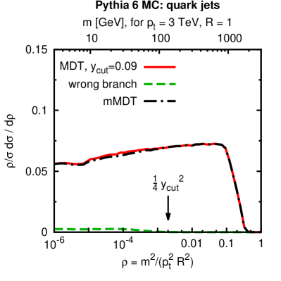
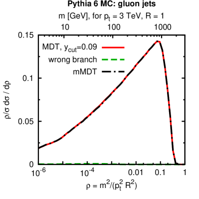
Figure 9: The MDT mass distribution, from Monte Carlo simulation (same as Fig. 1), with the contribution originating from wrong branches shown as a dashed line. Wrong branches are those for which, at some stage during the declustering, the tagger followed a prong whose $m^{2}+p_{t}^{2}$ was smaller than that of its partner prong.

While the wrong branch issue is numerically small, it is an undesirable characteristic of the MDT and calls for being eliminated. Rather than pursuing a full (and non-trivial) calculation of the resummed mass distribution for the MDT, we therefore propose in the next section that the MDT be modified.

7 Modified Mass-Drop Tagger

The modification of the mass-drop tagger that we propose is to replace step 3 of the definition on p. 3, with

1. Otherwise redefine $j$ to be that of $j_{1}$ and $j_{2}$ with the larger transverse mass ($m^{2}+p_{t}^{2}$) and go back to step 1 (unless $j$ consists of just a single particle, in which case the original jet is deemed untagged).

At leading order, since there is no recursion, this modified MDT (mMDT) behaves identically to the original MDT. However, in the case of configurations like those of Fig. 8b, the tagger will follow the $j_{1}$ branch rather than the $j_{23}$ branch thus eliminating the wrong-branch issues and the associated terms in Eq. (34).

Fig. 9 includes the tagged-mass spectrum from the modified mass-drop tagger in Monte Carlo simulation. One sees that, phenomenologically, the modification is a minor one, as can be checked also on events where the jet stems from a resonance decay (i.e. signal rather than background).

7.1 All-order tagged-mass distribution

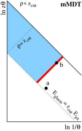
Figure 10: Lund kinematic diagram for the modified Mass-Drop Tagger (mMDT), concentrating on the region $\rho<z_{\text{cut}}$. The emissions labelled $a$ and $b$ are relevant to the discussion of angular versus mass ordering and the treatment of terms involving powers of $\alpha_{s}\ln^{2}y_{\text{cut}}$.

Not only does the mMDT eliminate the wrong-branch issue, but it also turns out to greatly facilitate the resummation of the tagged mass distribution.

As usual, we will work in the limit in which $y_{\text{cut}}$ is small, but $\alpha_{s}\ln y_{\text{cut}}$ is also small. To avoid complicating our formulae with excessive $\Theta$-functions, we will only quote explicit results in the plateau region of the LO calculation, i.e. $\rho<y_{\text{cut}}$. For $\rho>y_{\text{cut}}$, one simply obtains the plain jet-mass distribution.

It is useful to carry out the calculation in an angular ordered formulation, reflecting the inherent angular ordering that is present in the unclustering sequence followed by the tagger, a consequence of the fact that it is based on the C/A algorithm. We consider any number $n$ of emissions, strongly ordered in angle, $\theta_{i}\ll\theta_{i-1}$, in configurations such that the $n^{\text{th}}$ emission has a momentum fraction greater than $y_{\text{cut}}$, while all the others, at larger angles, have momentum fractions smaller than $y_{\text{cut}}$. The latter are simply unclustered and discarded by the mMDT and it is only when it reaches gluon $n$, the first with a momentum fraction greater than $y_{\text{cut}}$, that it tags the structure. This leads to the following all-order result for the mass distribution:

$$\frac{1}{\sigma}\frac{d\sigma}{d\rho}^{\text{(mMDT)}}=\sum_{n=1}^{\infty}\int\frac{\alpha_{s}C_{F}}{\pi}dz_{n}\,p_{gq}(z_{n})\frac{d\theta_{n}^{2}}{\theta_{n}^{2}}\Theta\left(z_{n}-y_{\text{cut}}\right)\delta\left(\rho-z_{n}\frac{\theta_{n}^{2}}{R^{2}}\right)\Theta(\theta_{n-1}-\theta_{n})\\ \times\prod_{i=1}^{n-1}\int\frac{\alpha_{s}C_{F}}{\pi}dz_{i}\,p_{gq}(z_{i})\frac{d\theta_{i}^{2}}{\theta_{i}^{2}}\left[\Theta\left(y_{\text{cut}}-z_{i}\right)-1\right]\Theta(\theta_{i-1}-\theta_{i})\,,$$ (37)

In this formula, $z_{i}$ is the fraction of energy carried by gluon $i$ relative to that of the original jet. Because $y_{\text{cut}}\ll 1$, all emissions $i<n$ carry away only a negligible fraction of the jet’s energy, so that one can consider the jet as always having the same energy even after multiple declusterings. As well as including real emissions, we have accounted for virtual corrections, the $-1$ contribution in the square brackets; from unitarity considerations, these can be treated as having the same phase-space integration as the real corrections, but obviously without the constraint $z_{i}<y_{\text{cut}}$ imposed by the mass drop tagger.

The terms in square brackets in Eq. (37) can be rewritten $-\Theta(z_{i}-y_{\text{cut}})$. This makes it clear that all the $z_{i}$ in the integrals are restricted to be larger than $y_{\text{cut}}$. Insofar as we neglect logarithms of $y_{\text{cut}}$, we can then replace the ordering of $\theta_{i}$ with an ordering in the variable $\rho_{i}\equiv z_{i}\theta^{2}_{i}/R^{2}$, allowing us to rewrite Eq. (37) in terms of integrals over (strongly) ordered $\rho_{i}$ values, i.e. $\rho_{i}<\rho_{i-1}$. The result for the integral of the $\rho$ distribution is then straightforward to express as an exponential,

$$\Sigma^{\text{(mMDT)}}(\rho) =\exp\left[-\int_{\rho}^{1}\frac{d\rho^{\prime}}{\rho^{\prime}}\int^{1}_{\max(y_{\text{cut}},\rho^{\prime})}dz\,p_{gq}(z)\frac{C_{F}}{\pi}\,\alpha_{s}(z\rho^{\prime}p_{t}^{2}R^{2})\right]\,,$$ (38a)

$$=\exp\left[-D(\max(y_{\text{cut}},\rho))-S(y_{\text{cut}},\rho)\Theta(y_{\text{cut}}-\rho)\right]$$ (38b)

where we have now explicitly written in the scale for the coupling and taken care of the modified $z$ integration limit for $\rho^{\prime}>y_{\text{cut}}$.

As usual, it can be convenient to examine Eq. (38) in the fixed coupling approximation. It is given by

$$\Sigma^{\text{(mMDT)}}(\rho)=\exp\left[-\frac{\alpha_{s}C_{F}}{\pi}\left(\ln\frac{y_{\text{cut}}}{\rho}\ln\frac{1}{y_{\text{cut}}}\,-\,\frac{3}{4}\ln\frac{1}{\rho}\,+\,\frac{1}{2}\ln^{2}\frac{1}{y_{\text{cut}}}\right)\right]\,,\quad(\text{for}\;\rho<y_{\text{cut}})\,,$$ (39)

which is simply the exponential of the integral of the LO result, Eq. (33).

Eq. (38) corresponds to evaluating the probability for excluding the shaded region shown in Fig. 10. From this, and the explicit fixed-coupling form, Eq. (39), it is straightforward to see that the most logarithmically divergent term in $\Sigma^{\text{(mMDT)}}$ at any order in $\alpha_{s}$ is $\alpha_{s}^{n}L^{n}$, i.e. there are no terms beyond single logarithms. Considering that all other taggers had terms $\alpha_{s}^{n}L^{p}$ with $p$ up to $2n$ or $2n-1$, this is a striking result.

Note that the strong ordering approximation for $\rho_{i}$ values that is implicit in obtaining Eq. (38) is the main reason why we are able to neglect the effect of the mass-drop condition in the tagger: for $\mu$ not too small, each time that one unclusters a subjet $j$ into a $j_{1}$ and $j_{2}$, if $z>y_{\text{cut}}$, then one knows that $m_{j_{1}}\ll m_{j}$ and so the mass-drop condition $m_{j_{1}}<\mu m_{j}$ is automatically satisfied. Of course, for finite $\mu$ values, there is a relative order $\alpha_{s}$ probability that $m_{j_{1}}>\mu m_{j}$, so causing the mass-drop condition to fail. Insofar as we control terms $\alpha_{s}^{n}\ln^{n}\rho$ in $\Sigma^{\text{(mMDT)}}$, this corresponds to corrections $\alpha_{s}^{n+1}\ln^{n}\rho$, which are beyond our accuracy.

It is interesting that Eq. (38), evaluated with a coupling that freezes in the infrared, tells us that every jet should be successfully mass-drop tagged, albeit possibly with a very small tagged mass. In practice, confinement modifies this picture and in Monte Carlo studies at hadron-level about 90% of jets pass the mMDT procedure.

So far we have concentrated on a limit where $y_{\text{cut}}\ll 1$, while at the same time neglecting logarithms of $y_{\text{cut}}$. It is interesting to explore what happens when we go beyond this limit. For sufficiently small $y_{\text{cut}}$, one might also aim to control terms $(\alpha_{s}\ln^{2}y_{\text{cut}})^{m}(\alpha_{s}\ln\rho)^{n}$ for any $m,n$. In this case a potential subtlety is that one should account for the difference between angular and mass ordering, because given some emission $a$ with $z>y_{\text{cut}}$, there is a probability $\sim\alpha_{s}\ln^{2}y_{\text{cut}}$ of having a second emission $b$ with $z>y_{\text{cut}}$, at a smaller angle than $a$ but contributing more than $a$ to the jet mass. Such a configuration is illustrated in Fig. 10. Here, emission $a$ will be unclustered before emission $b$. Its contribution to the squared mass $m_{a1}^{2}$ will in general be much smaller than that from $b$, $m_{b1}^{2}$. Consequently $m_{ab1}-m_{b1}\ll m_{ab1}$, i.e. there is no substantial mass drop when unclustering $a$. Emission $a$ is therefore discarded and it is only when $b$ is unclustered that the jet is tagged. This type of configuration might appear to complicate the treatment of the tagger, but actually it simply implies that it is irrelevant whether emission $a$ is present or not. For this reason, we believe that Eq. (38), written in terms of mass ordering, is correct for all terms $(\alpha_{s}\ln^{2}y_{\text{cut}})^{m}(\alpha_{s}\ln\rho)^{n}$. Accordingly, we have chosen to explicitly include terms that are subleading in a counting of powers of $\ln\rho$, but $\ln^{2}y_{\text{cut}}$-enhanced, in our expressions Eqs. (38), (39). We believe the result is identical also for $\mu=1$: there will be an infinitesimal mass drop when emission $a$ is unclustered, which is now sufficient to trigger the mass-drop condition; however, the masses $m_{ab1}$ and $m_{b1}$ differ little in most of the relevant phase space, so that once again it is irrelevant whether emission $a$ is present or not.

It is also possible to examine the mass-drop tagger for moderate $y_{\text{cut}}$ values. One of the key new features that arises at single-logarithmic accuracy in this limit is that one now discards emissions with moderate $z$, and these have a finite probability for modifying the flavour of the remaining hard prong. Therefore Eq. (38) needs to be extended to account for a matrix structure in flavour space. This, and other aspects of the moderate-$y_{\text{cut}}$ case, are discussed in detail in appendix B.

7.2 Absence of non-global logarithms

As we have already observed, there are no terms in the integrated tagged mass distribution of the form $\alpha_{s}^{n}\ln^{m}\rho$ with $m>n$. In other words, there is at most one logarithm of $\rho$ for each power of $\alpha_{s}$. It is to our knowledge the first time that a jet-mass type observable is found with this property. The reason that there are only single logarithms is that the mMDT completely removes contributions from soft emissions, i.e. one is left only with collinear divergences, but not soft-collinear ones, or pure soft ones.

The absence of pure soft divergences has a particularly interesting consequence, namely the absence of non-global logarithms. As we explained in section 3, non-global logarithms are potentially problematic. They typically arise from situations where a soft emission outside a (sub)jet emits a yet softer emission into the (sub)jet. Soft emissions inside the jet are systematically discarded by mMDT (or, in the situations where they’re kept, don’t affect the final tagged jet mass) and so the non-global logarithms are eliminated. The same mechanism ensures the absence of related “clustering” logarithms Appleby:2002ke ; Delenda:2006nf . This makes the mMDT particularly interesting, as the only infrared and collinear safe single-jet observable that can be straightforwardly calculated to single logarithmic accuracy with the full $N_{C}$ dependence. It also suggests that the mMDT should be given priority in calculations aiming for accuracy beyond single logarithms.

7.3 Comparison with Monte Carlo results

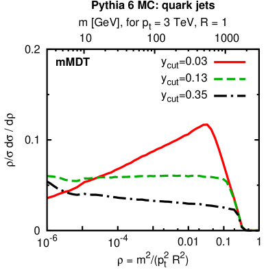
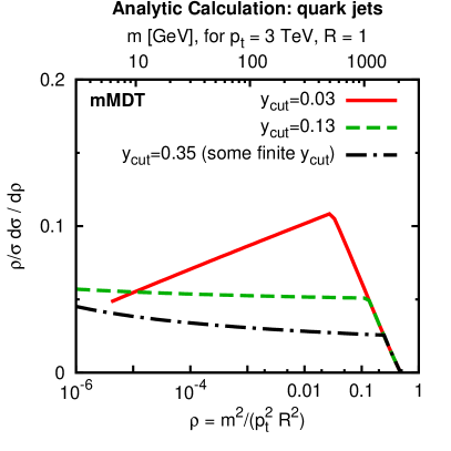
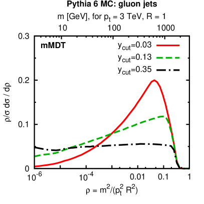
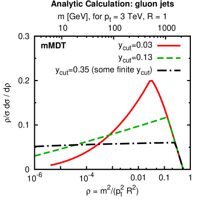
Figure 11: Comparison of Monte Carlo (left panels) and analytic results (right panels) for the modified mass-drop tagger (mMDT). The upper panels are for quark jets, the lower panels for gluon jets. Three values of $y_{\text{cut}}$ are illustrated, while $\mu$ is always taken to be $0.67$ (its precise value has no impact on the results, as long as it is not substantially smaller than this). The details of the MC event generation are as for Fig. 1.

Our analytical results are shown in Fig. 11 (right-hand plots) compared to parton-level Monte Carlo predictions with Pythia 6 (left, virtuality ordered shower). The upper panels show the results for quark jets, the lower panels for gluon jets. Three choices of $y_{\text{cut}}$ are shown. The agreement between Monte Carlo and the analytical results is striking. In particular, we note that there are two particular values of asymmetry parameter, namely $y_{\text{cut}}=0.13$ for quark-initiated jets, and $y_{\text{cut}}=0.35$ in the case of gluon-initiated jets, for which the mMDT mass distribution is essentially flat. We will come back to this observation in section 8.2, where we discuss background shapes in more detail.

Note that for the $y_{\text{cut}}=0.35$ choice, the analytical results have been supplemented with a subset of the finite $y_{\text{cut}}$ effects, specifically, those that are flavour-diagonal. Further details are given in appendix B. Residual small differences between the Monte Carlo and analytical results for $y_{\text{cut}}=0.13$ are in part due to the fact that we have left out finite $y_{\text{cut}}$ effects there.

7.4 Dependence on $\mu$ parameter

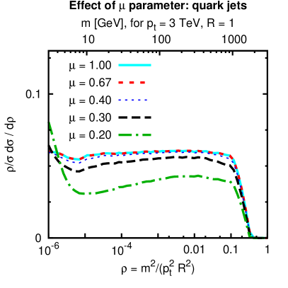
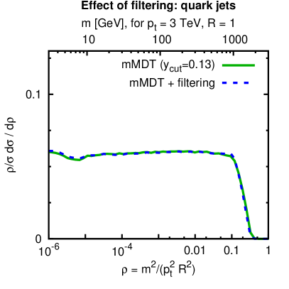
Figure 12: MC study of the impact of the mass-drop parameter ($\mu$) on the mMDT mass distribution (left panel) and of filtering (right panel) for quark jets. Filtering is carried out with $R_{\text{filt}}=\min(\frac{1}{2}\Delta_{12},0.3)$ and $n_{\text{filt}}=3$. The details of the MC event generation are as for Fig. 1. Gluon-initiated jets behave in a similar way.

As we have already discussed in section 7.1, the dependence of the mass-drop parameter $\mu$ enters beyond the single-logarithmic accuracy we achieve for mMDT. Fig. 12 (left panel) shows the results of a simple Monte Carlo study to numerically investigate the impact of the mass-drop parameter on the tagged mass distribution. One sees that for $0.4\lesssim\mu\leq 1$ there is essentially no dependence on $\mu$. For smaller values of $\mu$ the background tagging rate drops. This is caused by contributions that are subleading in terms of the number of logarithms of $\rho$, but enhanced by powers of $\ln^{2}\mu$, and associated with the Sudakov suppression for requiring that each of the two prongs of the tagged jet have a very small mass.

In light of these theoretical and Monte Carlo observations it seems that one could use mMDT entirely without any mass-drop condition. We believe that this simplification of the tagger deserves further investigation in view of possibly becoming the main recommended variant of mMDT.

7.5 Interplay with filtering

The mass-drop tagger is often used together with a filtering procedure, which reduces sensitivity to underlying event and pileup. In its original incarnation a filtering radius $R_{\text{filt}}$ was chosen equal to $\min(\Delta_{12}/2,0.3)$ Butterworth:2008iy , where $\Delta_{12}$ is the angular separation between the two prongs of the jet after tagging (for brevity, we call this the tagged jet). The tagged jet was then reclustered with radius $R_{\text{filt}}$, and only its $n_{\text{filt}}$ hardest prongs are kept.

From the point of a general analytical discussion of the effect of filtering, it is immaterial whether one use $R_{\text{filt}}=\min(\Delta_{12}/2,0.3)$ or simply some moderate fixed fraction of $\Delta_{12}$. What matters more is the choice of $n_{\text{filt}}$: for a tagged jet with $n$ particles, filtering will always leave the jet unmodified if $n\leq n_{\text{filt}}$. It is only if the jet has more than $n_{\text{filt}}$ subprongs on an angular scale $R_{\text{filt}}$ that filtering will change its mass. This occurs with relative probability $\alpha_{s}^{n_{\text{filt}}-1}$ (e.g. for $n_{\text{filt}}=3$ there must be at least two additional gluons in order for filtering to discard anything).

Naively one would therefore think that filtering introduces a modification at order N${}^{n_{\text{filt}}-1}$LL. However one should keep in mind that filtering doesn’t cause the jet to be discarded, but instead simply changes its mass. Suppose, for instance, that it reduces the mass by some factor $f$ with a probability $\alpha_{s}^{n_{\text{filt}}-1}$. Given a pre-filtering integrated mass distribution of $\Sigma(\rho)=\sum_{n}c_{n}\alpha_{s}^{n}L^{n}$, the post-filtering distribution will be

$$\Sigma^{\text{(filt)}}(\rho) =\Sigma(\rho)+\alpha_{s}^{n_{\text{filt}}-1}\left(\Sigma(\rho/f^{2})-\Sigma(\rho)\right)$$ (40a)

$$=\sum_{n}c_{n}\alpha_{s}^{n}L^{n}+\sum_{n}c_{n}\alpha_{s}^{n_{\text{filt}}+n-1}\left[(L+2\ln f)^{n}-L^{n}\right]$$ (40b)

The right-hand term of Eq. (40b) goes as $\alpha_{s}^{n_{\text{filt}}+n-1}L^{n-1}$, i.e. it is N${}^{n_{\text{filt}}}$LL. Accordingly, with the common choice $n_{\text{filt}}=3$, it is unlikely that there will be a need to perturbatively calculate filtering’s impact on the background in the near future!

We can verify this conclusion numerically with the help of a Monte Carlo study. This is shown in Fig. 12 (right), where mMDT mass distributions are compared with and without filtering, using $n_{\text{filt}}=3$. The difference between them is hardly perceptible.

7.6 Calculability at fixed order

An interesting consequence of the presence of only single logarithms relates to the extent to which fixed-order calculations are reliable. For observables with terms $\alpha_{s}^{n}L^{2n}$, fixed-order perturbation theory breaks down when $L\sim 1/\sqrt{\alpha_{s}}$ and becomes unreliable somewhat earlier. Instead, for observables whose most divergent terms are $\alpha_{s}^{n}L^{n}$, the breakdown occurs when $L\sim 1/\alpha_{s}$, i.e. fixed-order perturbation theory has a parametrically larger domain of applicability. We have not investigated the behaviour of the fixed-order predictions in detail, however such a study would be worthwhile and is straightforward to perform to NLO in the jet mass distribution with tools such as MCFM Campbell:2002tg and NLOJet++ Nagy:2003tz .

8 Phenomenological considerations

8.1 Comparisons between taggers

We have commented in previous sections on similarities between the taggers for regions of intermediate tagged mass. In particular if one chooses $y_{\text{cut}}=\frac{z_{\text{cut}}}{1-z_{\text{cut}}}$, then one expects trimming and pruning to be nearly identical to mMDT in the regions $\rho>z_{\text{cut}}(R_{\text{sub}}/R)^{2}$ and $\rho>z_{\text{cut}}^{2}$ respectively.

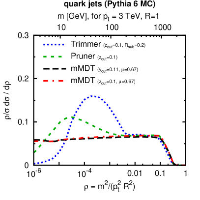
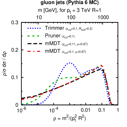
Figure 13: Comparisons of Monte Carlo distributions for trimming, pruning and mMDT for equivalent parameters, i.e. identical $z_{\text{cut}}=0.1$ for trimming and pruning, while for mMDT we use $y_{\text{cut}}=z_{\text{cut}}/(1-z_{\text{cut}})$. We also show the $z_{\text{cut}}$-variant of mMDT defined in the text, with $z_{\text{cut}}=0.1$. The details of the MC event generation are as for Fig. 1.

Choosing $y_{\text{cut}}=0.11$ and $z_{\text{cut}}=0.1$, this feature is evident in Fig. 13. There are remaining small differences between the tools, and in particular in the gluon case, for $\rho<z_{\text{cut}}$ one sees that trimming and pruning are closer to each other than either is to mMDT. With the help of further Monte Carlo studies, we have traced the difference to fact that both trimming and pruning directly cut on transverse momentum fractions (albeit normalised slightly differently), while mMDT cuts on a ratio of a $k_{t}$-distance to a mass, which only indirectly translates to a cut on momentum fractions. If, for instance, in step 2 of the definition of (m)MDT one replaces the cut $y=\min(p_{tj_{1}}^{2},p_{tj_{2}}^{2})\Delta R_{j_{1}j_{2}}^{2}/m_{j}^{2}>y_{\text{cut}}$ with $\min(p_{tj_{1}},p_{tj_{2}})/(p_{tj_{1}}+p_{tj_{2}})>z_{\text{cut}}$, then the small differences between mMDT and pruning in the region $\rho>z_{\text{cut}}^{2}$ disappear almost entirely, as can be seen. It is straightforward to show that this change does not affect the resummation at the order we have considered.

These observations are important, because previous discussions that have commented on differences between groomers (e.g. Boost2010 ) were considering them with non-equivalent parameters. As we see here, a suitable choice of parameters is essential for the comparisons to be as informative as possible.

Among the groomers examined in Ref. Boost2010 , there was also filtering (without the mass-drop procedure and with a fixed $R_{\text{filt}}$). While we have not investigated plain filtering in a similar level of detail to trimming, pruning and mMDT, preliminary investigations suggest that it leads to a background jet mass distribution that is very similar to that for the plain jet mass, in particular as concerns the leading-log structure $\alpha_{s}^{n}L^{2n}$.

8.2 Background shapes

From the point of view of searches with a small signal-to-background ratio, the reliability of the prediction for the background and especially its shape is crucial.

The background may be predicted with the aid of perturbation theory, for which our resummation, merged with fixed-order calculations, would be the state-of-the-art. Alternatively, backgrounds may be predicted with data-driven methods. One example of such a method is to measure the background mass distribution to the left and right of an expected W/Z or H mass peak and use that to predict the background mass distribution in the peak location. One may also take the shape of the background for moderate $p_{t}$ jets, and attempt to use it to predict the shape for higher $p_{t}$ jets. From this point of view the structures present in the mass distribution are of importance: for example Sudakov peaks, as they appear in the normal jet mass, in trimming and in pruning, can considerably complicate data-driven methods: they prevent one from reliably interpolating the background between two sidebands, because the peak may lie over one of the sidebands, or even worse, in between them; they also make it more complicated to use a mass distribution at one $p_{t}$ to predict the distribution at another $p_{t}$, because Sudakov peak positions depend on the jet $p_{t}$.

The (modified) mass-drop tagger is particularly interesting in this respect for two reasons. Firstly it is free of Sudakov peaks. Secondly it has an interesting feature that can be seen by expanding Eq. (38) to second order in the coupling, restricting our attention to the region $\rho<y_{\text{cut}}$:

$$\frac{\rho}{\sigma}\frac{d\sigma}{d\rho}^{\text{(mMDT)}}=\frac{\alpha_{s}C_{F}}{\pi}\ln\frac{e^{-\frac{3}{4}}}{y_{\text{cut}}}\left[1+\frac{\alpha_{s}}{\pi}\ln\frac{1}{\rho}\left(\beta_{0}-C_{F}\ln\frac{e^{-\frac{3}{4}}}{y_{\text{cut}}}\right)+\cdots\right]$$ (41)

where $\beta_{0}=(11C_{A}-2n_{f})/12$. Relative to the LO formula, Eq. (33), running coupling effects (the $\beta_{0}$ term) cause the the distribution to increase for low $\rho$, while the exponentiation in Eq. (38) brings a (single-logarithmic) Sudakov type suppression. For a specific value of $y_{\text{cut}}$, $\exp(-\frac{3}{4}-\frac{\beta_{0}}{C_{F}})$ in the case of quark jets, those two effects cancel, leaving a mass spectrum that is to a good approximation independent of $\rho$, a property that is potentially valuable in data-driven background estimates. For $n_{f}=5$ the relevant $y_{\text{cut}}$ value is $y_{\text{cut}}=e^{-\frac{35}{16}}\simeq 0.11$. Note that this is determined in the small-$y_{\text{cut}}$ approximation, which is subject to corrections of relative ${\cal O}\left(y_{\text{cut}}\right)$. Those corrections lead to a slight increase of the critical $y_{\text{cut}}$ value that is needed for flatness, which is consistent with the practical observation of flatness for quark jets in Fig. 11 at $y_{\text{cut}}\simeq 0.13$.

Fig. 11 is also consistent with the expectation from Eq. (41) that for small $y_{\text{cut}}$ the mass distribution will tend to fall off towards small $\rho$, with the slope being dominated by the Sudakov term; conversely, for large $y_{\text{cut}}$ the distribution is more likely to increase towards small $\rho$, with the slope being dominated by the running-coupling term. For gluon jets the $C_{F}$ coefficients are replaced by $C_{A}$ (and $\frac{3}{4}$ by $\beta_{0}/C_{A}=\frac{23}{36}$). This causes the Sudakov-induced term to be relatively more important, hence the tendency to decrease more steeply towards small $\rho$ and the need for a larger $y_{\text{cut}}$ value in order to obtain a flat distribution.

8.3 Non-perturbative effects

While the main aim of this work has been to understand perturbative effects in the taggers, it is important to also be aware of the extent to which they may be affected by non-perturbative contributions.

8.3.1 Limit of perturbative calculation

One simple study is to determine, for each tagger, the non-perturbative transition point, below which our calculations start to probe the non-perturbative region. One can define the transition point as the highest mass for which the coupling, in any of the integrals, must be evaluated below some non-perturbative transition scale $\mu_{\text{NP}}$. One can imagine $\mu_{\text{NP}}$ to be of order $1\,\mathrm{GeV}$.

For the normal jet mass, the transition point can be evaluated by considering an emission $i$ with $E_{i}\theta_{i}=\mu_{\text{NP}}$. The squared jet mass is $m^{2}=E_{i}E_{\mathrm{jet}}\theta_{i}^{2}$ and so the transition point is found taking the largest possible value for $\theta$, which gives $m^{2}\simeq\mu_{\text{NP}}E_{\text{jet}}R$. In longitudinally-invariant variables, this reads

$$m^{2}\simeq\mu_{\text{NP}}\,p_{t,\text{jet}}\,R\,,\qquad\quad\text{(plain jet mass)}.$$ (42)

Note that this scale grows with the jet $p_{t}$, so that even apparently large masses, $m\gg\Lambda_{\text{QCD}}$, may in fact be driven by non-perturbative physics. For a $3\,\mathrm{TeV}$ jet with $R=1$, taking $\mu_{\text{NP}}=1\,\mathrm{GeV}$, the non-perturbative region corresponds to $m\lesssim 55\,\mathrm{GeV}$, disturbingly close to the electroweak scale!

To obtain the transition point for trimming, one simply replaces $R$ with $R_{\text{sub}}$, giving

$$m^{2}\simeq\mu_{\text{NP}}\,p_{t,\text{jet}}\,R_{\text{sub}}\,,\qquad\quad\text{(trimming)},$$ (43)

assuming that this lies in the region $\rho<r^{2}z_{\text{cut}}$, which usually will be the case for sufficiently high $p_{t}$ jets. For our canonical $3\,\mathrm{TeV}$, $R=1$ jet, taking $R_{\text{sub}}=0.2$ tells us that the non-perturbative region is $m\lesssim 25\,\mathrm{GeV}$.

For both Y- and I-pruning, the non-perturbative transition region is formally in the same location as for the plain jet mass. This is because of the integrals over $\rho_{\text{fat}}$, Eqs. (23), (25), whose lower limits can be as low as $\rho$. Note, however, that the onset of the non-perturbative effects may be substantially different, because the fraction of the answer that is associated with the non-perturbative region, as well as the interplay between real and virtual components, are different compared to the plain jet mass.

Finally, for the modified mass-drop tagger, we first observe that the smallest scale in the coupling will occur when the momentum fraction of the tagged splitting is $z\simeq y_{\text{cut}}$. The squared mass of the jet is then $m^{2}\simeq y_{\text{cut}}E_{\text{jet}}^{2}\theta^{2}$. Substituting the condition for the emission to be non perturbative, $y_{\text{cut}}^{2}E_{\text{jet}}^{2}\theta^{2}=\mu_{\text{NP}}^{2}$, leads to a transition point of

$$m^{2}\simeq\frac{\mu_{\text{NP}}^{2}}{y_{\text{cut}}}\,,\qquad\qquad\text{(mMDT)}.$$ (44)

Note that in contrast with the cases seen above, this transition point is independent of the jet $p_{t}$, and genuinely close to the non-perturbative region. Taking $y_{\text{cut}}=0.1$, it corresponds to a scale of about $3\,\mathrm{GeV}$.

8.3.2 Monte Carlo study of hadronisation

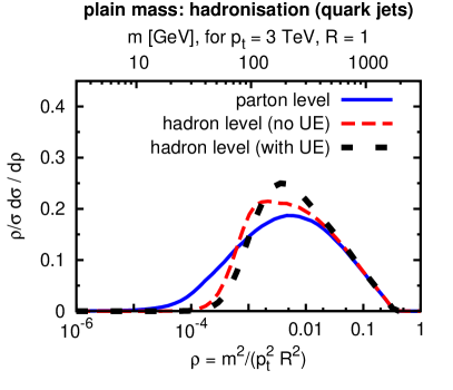
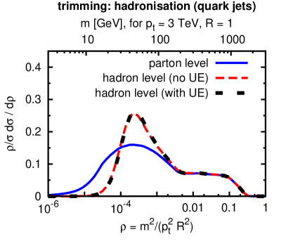
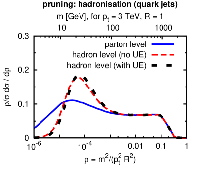
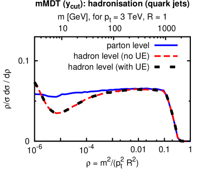
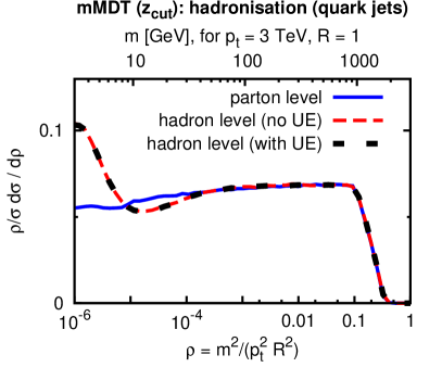
Figure 14: The impact of hadronisation and the underlying event (UE) on the mass spectra for different taggers. The details of the MC event generation are as for Fig. 1.

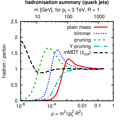
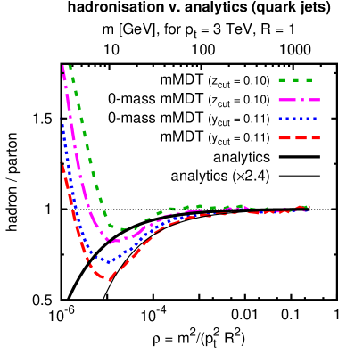
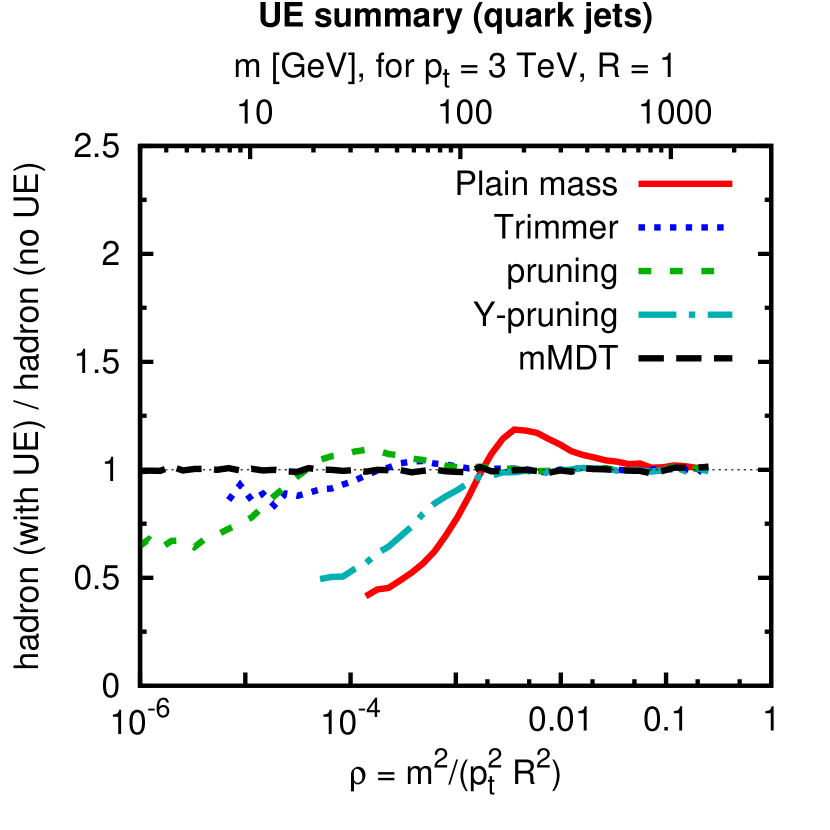
Figure 15: Top left: ratio of hadron-level (without UE) to parton level results for various groomers and taggers. Top right: ratio of hadron-level (without UE, both with finite and zero hadron masses) to parton level results for mMDT (with $y_{\text{cut}}$ and $z_{\text{cut}}$) and comparison to the analytic calculation of hadronisation corrections from section 8.3.3. Bottom: ratio of hadron levels with and without UE. The details of the MC event generation are as for Fig. 1.

It is instructive to supplement the above discussion with Monte Carlo studies of the effect of hadronisation. Figure 14 shows the mass distributions at parton-level, hadron-level without underlying event (UE) and hadron-level with UE, for plain jet mass, trimming, full and Y-pruning and mMDT using either a $y_{\text{cut}}$ or a $z_{\text{cut}}$. Figure 15 shows the corresponding ratios of hadron and parton-level distributions.

Let us first concentrate on the effect of hadronisation. For any given mass, the plain jet mass is the most strongly affected by hadronisation, with $25\%$ corrections even for jet masses of $100\,\mathrm{GeV}$, in the neighbourhood of the peak region. This scale is about twice that estimated as the limit of the perturbative calculation in section 8.3.1, which itself was large because it scales as $\sqrt{p_{t}}$, as given in Eq. (42).

We anticipated that trimming should only be affected by non-perturbative physics at a somewhat smaller mass than for ungroomed jets. This is indeed what we see (most clearly in the top left panel of Fig. 15). Still, trimming’s peak region is strongly affected, even more so than for the plain jet mass, which is a consequence of the non-trivial interplay between the change in perturbative peak position and the change in non-perturbative effects as one goes from plain to trimmed jet mass.

While pruning nominally has non-perturbative effects setting in at the same mass as the plain jet mass, we argued that their onset might in practice be somewhat different, as is indeed observed: it appears not too dissimilar to trimming. Y-pruning looks somewhat different because it doesn’t have a Sudakov peak, however from Fig. 15 it is clear that the order of magnitude of hadronisation effects is similar in full pruning and Y-pruning.

As expected, it is the mMDT that has the smallest hadronisation corrections, with non-trivial structure appearing at about $10\,\mathrm{GeV}$, about three times the scale estimated in section 8.3.1 for the limit of the perturbative calculation. The impact of hadronisation for mMDT depends somewhat on whether it is used with a $y_{\text{cut}}$ or $z_{\text{cut}}$, and for the latter in particular hadronisation remains very modest all the way down to $10\,\mathrm{GeV}$.

8.3.3 Analytic hadronisation estimate for mMDT

It is worthwhile examining whether the form of the onset of hadronisation for mMDT, above $10\,\mathrm{GeV}$, can be explained at least qualitatively. Multiple effects can play a role: for example, hadronisation was argued in Dasgupta:2007wa to shift a given jet’s squared mass by an amount $\delta m^{2}\simeq C\,\Lambda_{\text{NP}}\,p_{t}R$, where $C$ is either $C_{F}$ or $C_{A}$ and $\Lambda_{\text{NP}}\sim 0.4\,\mathrm{GeV}$. Hadronisation is also believed to change a jet’s (or a prong’s) momentum, shifting it by an amount $\delta p_{t}\simeq-C\Lambda_{\text{NP}}/R$ Korchemsky:1994is ; Dasgupta:2007wa . (The numbers are given here for the anti-$k_{t}$ algorithm with $R\ll 1$ and in the case of the jet mass assume a scheme in which hadron masses are neglected; the $p_{t}$ shift result for the $k_{t}$ algorithm is given in Ref. Dasgupta:2009tm ; the other cases, including for the C/A algorithm, have yet to be calculated).

For a tagger one needs to work out the interplay between hadronisation and the tagging procedure. For example, let us consider the shift in jet mass, in the case of a quark jet. The action of the tagger is such that the average effective radius of a tagged jet is a function of the tagged jet mass itself, $R_{\text{eff}}\sim f(y_{\text{cut}})m/p_{t}$, where

$$f(y_{\text{cut}})=\frac{\int_{y_{\text{cut}}}^{1-y_{\text{cut}}}dz\,p_{gq}(z)\left[z(1-z)\right]^{-\frac{1}{2}}}{\left.\int_{y_{\text{cut}}}^{1-y_{\text{cut}}}dz\,p_{gq}(z)\right.}\,,$$ (45)

for quark-initiated jets. For $y_{\text{cut}}\simeq 0.1$, $f(y_{\text{cut}})\simeq 2.5$. Thus we obtain

$$\delta m^{2}\simeq C_{F}\,f(y_{\text{cut}})\,\Lambda_{\text{NP}}\,m\,\qquad\longrightarrow\qquad\delta m\simeq\frac{1}{2}\,C_{F}\,f(y_{\text{cut}})\,\Lambda_{\text{NP}}\,.$$ (46)

For cases where $d\sigma/dm$ scales as $1/m$, this leads to a correction

$$\frac{d\sigma}{dm}^{\text{NP}}=\frac{d\sigma}{dm}^{\text{PT}}\left(1+\frac{1}{2}\,C_{F}\,f(y_{\text{cut}})\,\frac{\Lambda_{\text{NP}}}{m}\right)\,.$$ (47)

Next, let us consider the effect of the $p_{t}$ shift. This is most relevant in cases where one of the prongs, at parton level, has a momentum such that it just passes the $y_{\text{cut}}$ asymmetry requirement. After hadronisation its $p_{t}$ is reduced, and so it may no longer pass that requirement. That leads to a drop in efficiency, which can be evaluated as follows. The effect will be relevant for asymmetric splittings, where the softer prong’s momentum fraction is $z\sim y_{\text{cut}}$. The effective jet radius will be of order $\frac{m}{p_{t}}y_{\text{cut}}^{-\frac{1}{2}}$, and so the absolute change in the prong’s $p_{t}$ will be $-C_{A}\Lambda_{\text{NP}}y_{\text{cut}}^{1/2}\frac{p_{t}}{m}$. This leads to a change in the momentum fraction (relative to original jet) for the softer prong of $-C_{A}\frac{\Lambda_{\text{NP}}}{m}y_{\text{cut}}^{1/2}$. Note the $C_{A}$ colour factor here, since the soft prong will almost always be a gluon. Given that the perturbative tagging efficiency is equal to the integral over the splitting function down to momentum fractions $\simeq y_{\text{cut}}$, the non-perturbative correction can be evaluated by estimating how the integral changes when requiring a momentum fraction greater than $y_{\text{cut}}+C_{A}\frac{\Lambda_{\text{NP}}}{m}y_{\text{cut}}^{1/2}$. This gives us

$$\frac{d\sigma^{\text{NP}}}{dm} \simeq\frac{d\sigma^{\text{PT}}}{dm}\;\frac{\ln\left(y_{\text{cut}}+C_{A}\frac{\Lambda_{\text{NP}}}{m}y_{\text{cut}}^{1/2}\right)+\frac{3}{4}}{\ln y_{\text{cut}}+\frac{3}{4}}\,,$$ (48a)

$$\simeq\frac{d\sigma^{\text{PT}}}{dm}\;\left(1-C_{A}\frac{y_{\text{cut}}^{-1/2}}{\ln 1/y_{\text{cut}}-\frac{3}{4}}\,\frac{\Lambda_{\text{NP}}}{m}\right).$$ (48b)

One element that we have neglected here is that if hadronisation causes a (sub)jet with mass $m_{1}$ to fail the $y_{\text{cut}}$ (or $z_{\text{cut}}$) requirement, then mMDT continues to recurse into the harder prong. This will populate the lower mass region and the jet might then tagged as having mass $m_{2}\ll m_{1}$. The contribution from this effect to masses of order $m_{2}$ will be proportional to $\alpha_{s}\Lambda_{\text{NP}}/m_{1}$, whereas the direct correction to masses of order $m_{2}$ will be proportional to $\Lambda_{\text{NP}}/m_{2}$, which is parametrically larger.

The dependence of the hadronisation correction on $m$ is identical in Eqs. (47) and (48), with only the coefficient changing. Interestingly the corrections depend just on the jet mass, and not on the jet $p_{t}$; this is characteristically different from the situation for plain jet mass.

Numerically it is the negative contribution from the $p_{t}$ shift that dominates over the mass shift. Considerable caution is needed, however, as concerns the actual numerical prediction from these formulae: we have ignored hadron-mass effects, which are known to be substantial Salam:2001bd ; Mateu:2012nk ; we have ignored the (complicated) issue that the two-pronged structure of the jet will undoubtedly modify the pattern of hadronisation corrections relative to the calculations of Dasgupta:2007wa , both for the overall jet mass and the prong transverse momentum; we have also ignored the differences between mMDT with a $y_{\text{cut}}$ and a $z_{\text{cut}}$, even though we have seen that they have different non-perturbative effects, possibly because $y$’s definition involves the jet mass, which is itself subject to further corrections. Accordingly, it is probably only the overall $\Lambda_{\text{NP}}/m$ scaling in Eqs. (47) and (48) that can be considered robust.

Despite these caveats, it is still interesting to compare the result of Eqs. (47) and (48) to the Monte Carlo results. This is done in the top-right plot of Fig. 15. The plot shows the Monte Carlo results for both the $y_{\text{cut}}$- and $z_{\text{cut}}$-based mMDT. For the results labelled “0-mass,” all particles’ 4-momenta have been transformed (before clustering) so as to have zero mass, while maintaining their $p_{t}$, rapidity and azimuth. The figure also shows our analytical result, as well as a variant where the hadronisation corrections have been rescaled by an (arbitrarily chosen) factor of $2.4$. All the Monte Carlo results seem to be roughly consistent with our predicted $\Lambda_{\text{NP}}/m$ scaling down to ${\cal O}\left(10\,\mathrm{GeV}\right)$. However the normalisation of the hadronisation correction appears to be very sensitive to the details of the tagger and the input particles. The version of mMDT formulated in terms of a $z_{\text{cut}}$ and with massless input particles appears to agree reasonably well with our prediction. This may just be a coincidence, though it is also true that this is the variant for which our estimates above were most likely to be reasonable.

A final comment concerns the absolute size of the hadronisation corrections for the $z_{\text{cut}}$-based mMDT variants: in the region of phenomenological interest, it seems that hadronisation is just a couple of percent. This suggests that these mMDT variants may be optimally suited to high-precision studies, both in new physics searches, and possibly also even applications such measurements of the strong coupling.

8.3.4 Underlying event

A discussion of non-perturbative effects would not be complete without considering the underlying event (UE), whose impact for each tagger can be seen in Fig. 14, with a summary in the bottom plot of Fig. 15. The jet mass is the most strongly affected, while all the groomed/tagged results show a significantly reduced UE sensitivity, which was part of the intention in their design. For trimming and pruning this sensitivity remains genuinely small throughout the phenomenologically relevant region, and in particular significantly smaller than the hadronisation corrections. For mMDT the dependence on UE is almost imperceptible, at or below the $1\%$ level for all jet masses.

For Y-pruning the UE sensitivity is not negligible: this is because the UE can significantly increase the original jet’s mass and the resulting pruning radius. Consequently, a jet that was classified as Y-pruned without UE, may be reclassified as I-pruned. The overall pruning rate increases slightly (because for I-pruned jets the $z$-cut is turned off), while the Y-pruned rate is noticeably decreased. This sensitivity to UE is perhaps the one main disadvantage of Y-pruning, and is, we believe, inherent to any approach that effectively relies on the original jet mass to help discriminate between colour singlet signals and colour triplet/octet backgrounds.

One should be aware that the above pattern of UE dependence does depend on the jet transverse momentum. For example, mMDT was originally designed in conjunction with filtering in order to reduce the effect of UE. This appears not to be necessary here, but had we considered jets with transverse momentum of a couple of hundred GeV, as was the context for the original MDT+filtering study, then the much larger effective radius for the tagged jet would have led to noticeable UE effects in the absence of filtering.

8.4 Choice of Monte Carlo Generator

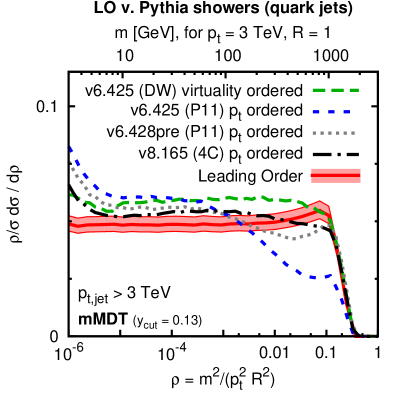
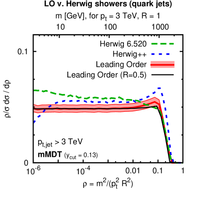
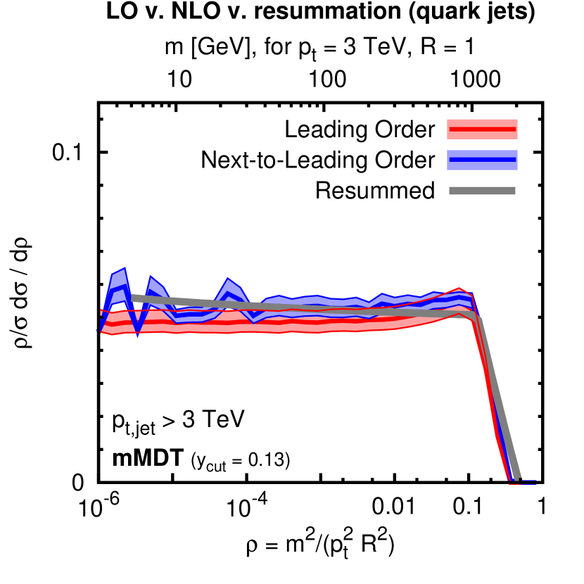
Figure 16: Mass distributions for mMDT tagged jets, comparing different parton-shower generators, the resummation and the exact leading-order and next-to-leading order results (obtained with NLOJet++ Nagy:2003tz with the MSTW2008 NLO PDF set Martin:2009iq ), with a central scale choice $\mu_{R}=\mu_{F}=p_{t}$ and simultaneous scale variations by a factor of two. Unless otherwise specified the curves correspond to a jet radius of $R=1$. The Monte Carlo results have been obtained at parton level, with the underlying event turned off. See text for further details.

Throughout this work, we have regularly compared our analytical results for the tagged mass distributions with the output of Monte Carlo parton shower simulations from Pythia 6.425 Pythia6 , with the DW tune DW of its virtuality-ordered shower. We have generally found good agreement between our analytics and the Pythia parton-shower simulations. It is also of interest to check whether the agreement is equally good when using different parton showers. To do so, we concentrate on the mMDT mass distribution, in the case of quark-initiated jets, for $y_{\text{cut}}=0.13$, at the parton level.

The top-left plot of figure 16 shows the comparison between the different showers in Pythia 6 and Pythia 8: the virtuality-ordered one in Pythia 6, our default, and the $p_{t}$-ordered one in Pythia 6 PythiaPtOrdered (in the Perugia 2011 Skands:2010ak tune) and the $p_{t}$-ordered shower from Pythia 8 Pythia8 (in the 4C tune Corke:2010yf ). The top-right plot shows the mMDT mass distribution obtained with the angular-ordered showers from Herwig 6.520 Corcella:2002jc and Herwig++ 2.6.3 Herwig++ ; Arnold:2012fq ; Lonnblad:1998cq in their default tunes. The Monte Carlo curves are obtained with a generation cut of $p_{t}>2.2\,\mathrm{TeV}$ applied to the $qq\to qq$ hard process, and the tagging analysis is then carried out on all jets with $p_{t}>3\,\mathrm{TeV}$. All plots include the full leading order (LO) result obtained with the program NLOJet++ Nagy:2003tz . The fixed-order calculation is important in that it enables us to check the distributions for large masses, where resummation may not be appropriate. We ensure a high purity of quark-initiated jets in the fixed-order calculations by setting the incoming gluon parton distribution functions to zero.

The plots in the top row figure 16 show that nearly all the Monte Carlo generators are in reasonable agreement with each other, with our resummation and with the LO calculation. The one exception is the $p_{t}$-ordered shower in Pythia 6.245, which predicts a noticeably different shape for the distribution, both at small and large masses. We have checked that this characteristic holds also in another widespread tune of the $p_{t}$-ordered shower, Z2 Field:2010bc . This significant difference relative to our calculations and the other generators appears to be limited to situations where the jet transverse momenta are close to the kinematic limit. We have checked that similar differences appear also for the other substructure tools considered in this paper. Following discussions with the authors of Pythia, they provided us with code for a modified version of the $p_{t}$-ordered shower, which resolves an issue in which the hardness of the final-state shower could be affected by the presence (or not) of soft initial-state emissions. Results with this modified shower are shown in Fig. 16 (top-left) as a dotted curve, labelled v6.428pre, and one observes a clear improvement in the agreement with other tools. This example illustrates the value of analytical understanding in situations such as this where Monte Carlo results from various generators differ noticeably.

We note that the LO curve exhibits non-trivial structure (a small bump) in the vicinity of $\rho=0.1$. This structure is absent in most of the Monte Carlo results, as well as in the results obtained from our analytical calculation (it is however present for Herwig++, and somewhat stronger than in the LO result). We believe that it is driven by the precise structure of hard large-angle radiation: this can be thought of as having a significant hard initial-state radiation contribution, neglected in our calculations and only approximately present in the parton showers. To confirm this hypothesis we also show the LO calculation for a jet of radius $R=0.5$ (left-hand plot), which should reduce the initial-state radiation contribution. Indeed, the structure at $\rho\simeq 0.1$ is much less pronounced. We expect that if we had carried out simulations with tools such as MC@NLO Frixione:2002ik or POWHEG Nason:2004rx (or alternatively CKKW Catani:2001cc or MLM Alwall:2007fs matching), these would have correctly accounted for this type of large-mass structure, without significantly modifying the results at lower $\rho$. It would be interesting to verify this expectation, however such a study is beyond the scope of this work.

Finally, the bottom-left plot shows our resummed prediction and the NLO result. As discussed in section 8.2, the choice $y_{\text{cut}}=0.13$ minimises higher-order corrections and hence the all-order result is dominated by the LO contribution, even at relatively small masses. This property is confirmed in the NLO calculation, whose central value is just within the scale uncertainty band of the LO calculation.

8.5 Effect of the taggers on signal–background discrimination

We have so far considered only the question of how the various taggers/groomers behave for backgrounds, i.e. quark or gluon-induced jets. A key question for evaluating the performance of taggers is also that of how they fare on signal jets, for example $W$, $Z$ or Higgs-bosons. The basic, known tree-level result, is that for the decay of a scalar particle, the tagging efficiency of a tagger like mMDT is essentially

$$\epsilon_{S}=\int_{z_{\text{cut}}}^{1-z_{\text{cut}}}dz\;P_{H\to q\bar{q}}(z)=1-2z_{\text{cut}}\,,$$ (49)

where the results makes use of the fact that $P_{H\to q\bar{q}}(z)=1$. As usual, in the small $z_{\text{cut}}$ limit, $y_{\text{cut}}$ and $z_{\text{cut}}$ are interchangeable. The same result holds for pruning (original and Y-pruning), modulo corrections associated with initial-state radiation (ISR). For trimming, the result depends on $m/p_{t}$, and is $1-2z_{\text{cut}}$ for $\rho>z_{\text{cut}}r^{2}$ and tends to $1$ for asymptotically smaller $m/p_{t}$ (again, modulo corrections from ISR). Of course, the tagging always needs to be performed in a given mass window, and these estimates assume that the mass window is sufficiently wide relative to any loss of mass resolution caused by ISR, UE and pileup (the width was studied in detail for MDT with filtering by Rubin in Ref. Rubin:2010fc ).

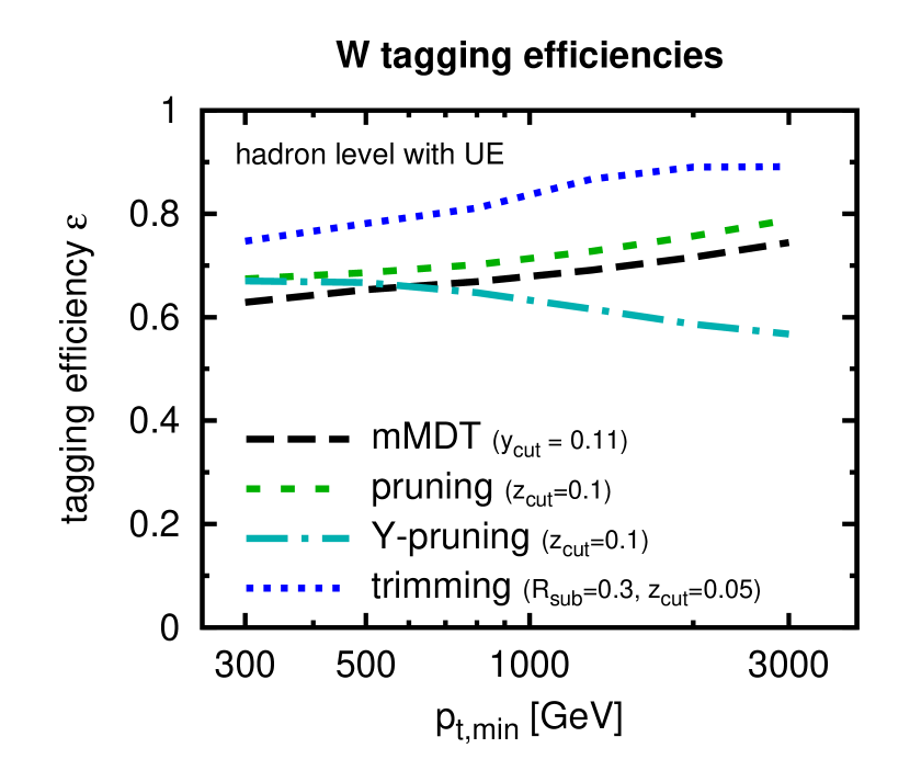
Figure 17: Efficiencies for tagging hadronically-decaying $W$’s, for a range of taggers/groomers, shown as a function of the $W$ transverse momentum generation cut in the Monte Carlo samples (Pythia 6, DW tune). Further details are given in the text.

Fig. 17 shows tagging efficiencies obtained with Pythia 6 (DW tune) at hadron level (with UE). They have been obtained in $WZ$ events, with the $Z$ decaying leptonically and the $W$ hadronically. The tagger is applied to the hardest jet in the event, which is deemed tagged if its final mass is in the window $64$–$96\,\mathrm{GeV}$. The fraction of jets that were tagged is shown as a function of a minimum $p_{t}$ cut applied on the $q\bar{q}\to WZ$ hard event in the simulation. As expected, the tagging efficiencies are fairly independent of the $p_{t,\min}$ choice, and reasonably consistent with the $1-2z_{\text{cut}}$ expectation. The differences that one sees relative to that expectation have two main origins. Firstly Eq. (49) holds at tree-level. It receives ${\cal O}\left(\alpha_{s}\right)$ corrections from gluon radiation off the $W\to q\bar{q}^{\prime}$ system. Monte Carlo simulation suggests these effects are responsible, roughly, for a $10\%$ reduction in the tagging efficiencies. Secondly, Eq. (49) was for unpolarized decays. By studying leptonic decays of the $W$ in the $pp\to WZ$ process, one finds that the degree of polarization is $p_{t}$ dependent, and the expected tree-level tagging-efficiency ranges from about $76\%$ at low $p_{t}$ to $84\%$ at high $p_{t}$. These two effects explain the bulk of the modest differences between Fig. 17 and the result of Eq. (49). However, the main conclusion that one draws from Fig. 17 is that the ultimate performance of the different taggers will be driven by their effect on the background rather than by the fine details of their interplay with signal events. This provides an a posteriori justification of our choice to concentrate our study on background jets.

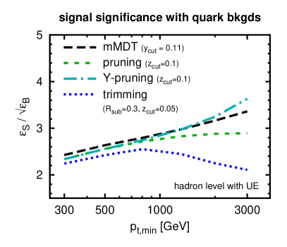
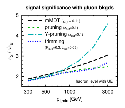
Figure 18: The significance obtained for tagging signal ($W$’s) versus background, defined as $\epsilon_{S}/\sqrt{\epsilon_{B}}$, for a range of taggers/groomers, shown as a function of the transverse momentum generation cut in the Monte Carlo samples (Pythia 6, DW tune) Further details are given in the text.

Figure 18 shows the overall performance of the different taggers quantified as $S=\epsilon_{S}/\sqrt{\epsilon_{B}}$, which is proportional to the signal significance that can be obtained with a given tagger. Here $\epsilon_{B}$ is the fraction of quark (left plot) or gluon (right plot) jets that are tagged and pass the mass cut.

Let us start by discussing mMDT. Its signal significance $S$ grows with $p_{t}$. This is driven by three modest effects combining together: the signal efficiency increases at high $p_{t}$; the background tagging rate is, in a first approximation, proportional to $\alpha_{s}(p_{t})$, which decreases at high $p_{t}$; and for our choice $y_{\text{cut}}=0.11$, the tagging rate decreases slightly for decreasing $m/p_{t}$ (cf. Fig. 11). The signal significance is lower for gluon backgrounds than for quark backgrounds, which is simply a consequence of the $C_{A}$ v. $C_{F}$ colour factor in the leading-order background tagging rate. This is partially compensated for at high $p_{t}$ by the steeper $m/p_{t}$ dependence in the gluon case.

Next, consider trimming. At low $p_{t}$ it has a slightly lower significance than mMDT, mainly because the particular $z_{\text{cut}}$ we’ve used is slightly non-optimal for tagging purposes. However, its main relevant feature is the drop in significance relative to the mMDT curve for $p_{t}\gtrsim 800\,\mathrm{GeV}$. This corresponds to a $\rho$ value of $0.01$, which is to be compared to the point $\rho=r^{2}z_{\text{cut}}=0.0045$ in Eqs. (8), (13) at which the background starts to grow and develop a low-mass Sudakov peak. cf. Eq. (13). The departure from mMDT is less pronounced in the gluon case than in the quark case because the stronger Sudakov suppression from the $C_{A}$ colour factor reduces the height of the low-mass background Sudakov peak.

Finally, we examine pruning. Like trimming, pruning has a low-mass Sudakov peak, but it develops only for lower masses than for trimming, and accordingly the drop in performance of pruning relative to mMDT is mitigated. Most interesting, perhaps, is Y-pruning. Its background enjoys a double-logarithmic Sudakov suppression for small $m/p_{t}$, due to the factor $e^{-D(\rho)}$ in Eq. (24a). The analogous effect for the signal is, we believe, single-logarithmic, hence the modest reduction in signal yields in Fig. 17. Overall the background suppression dominates, leading to improved tagging significance at high $p_{t}$. This is most striking in the gluon case, because of the $C_{A}$ colour factor in the $e^{-D(\rho)}$ Sudakov suppression. Despite this apparent advantage, one should be aware of a defect of Y-pruning, namely that at high $p_{t}$ the Y/I classification can be significantly affected by underlying event and pileup, because of the way in which they modify the original jet mass and the resulting pruning radius. It remains of interest to develop a tagger that exploits the same double-logarithmic background suppression while not suffering from this drawback.

9 Conclusions

	highest logs	transition(s)	Sudakov peak	NGLs	NP: $m^{2}\lesssim$
plain mass	$\alpha_{s}^{n}L^{2n\phantom{-1}}$	—	$L\simeq 1/\sqrt{{\bar{\alpha}}_{s}}$	yes	$\mu_{\text{NP}}\,p_{t}\,R$
trimming	$\alpha_{s}^{n}L^{2n\phantom{-1}}$	$z_{\text{cut}}$, $r^{2}z_{\text{cut}}$	$L\simeq 1/\sqrt{{\bar{\alpha}}_{s}}-2\ln r$	yes	$\mu_{\text{NP}}\,p_{t}\,R_{\text{sub}}$
pruning	$\alpha_{s}^{n}L^{2n\phantom{-1}}$	$z_{\text{cut}}$, $z_{\text{cut}}^{2}$	$L\simeq 2.3/\sqrt{{\bar{\alpha}}_{s}}$	yes	$\mu_{\text{NP}}\,p_{t}\,R$
MDT	$\alpha_{s}^{n}L^{2n-1}$	$y_{\text{cut}}$, $\frac{1}{4}y_{\text{cut}}^{2}$, $y_{\text{cut}}^{3}$	—	yes	$\mu_{\text{NP}}\,p_{t}\,R$
Y-pruning	$\alpha_{s}^{n}L^{2n-1}$	$z_{\text{cut}}$	(Sudakov tail)	yes	$\mu_{\text{NP}}\,p_{t}\,R$
mMDT	$\alpha_{s}^{n}L^{n\phantom{2-1}}$	$y_{\text{cut}}$	—	no	$\mu_{\text{NP}}^{2}/y_{\text{cut}}$

Table 1: Table summarising the main features for the plain jet mass, the three original taggers of our study and the two variants introduced here. In all cases, $L=\ln\frac{1}{\rho}=\ln\frac{R^{2}p_{t}^{2}}{m^{2}}$, $r=R_{\text{sub}}/R$ and the log counting applies to the region below the smallest transition point. The transition points themselves are given as $\rho$ values. Sudakov peak positions are quoted for $d\sigma/dL$; they are expressed in terms of ${\bar{\alpha}}_{s}\equiv\alpha_{s}C_{F}/\pi$ for quark jets and ${\bar{\alpha}}_{s}\equiv\alpha_{s}C_{A}/\pi$ for gluon jets and neglect corrections of ${\cal O}\left(1\right)$. “NGLs” stands for non-global logarithms. The last column indicates the mass-squared below which the non-perturbative (NP) region starts, with $\mu_{\text{NP}}$ parametrising the scale where perturbation theory is deemed to break down.

In this paper we have developed an extensive analytical understanding of the action of widely used boosted-object taggers and groomers on quark and gluon jets.

We initially intended to study three methods: trimming, pruning and the mass-drop tagger (MDT). The lessons that we learnt there led us to introduce new variants, Y-pruning and the modified mass-drop tagger (mMDT). The key features of the different taggers are summarised in table 1. We found, analytically, that the taggers are similar in certain phase-space regions and different in others, identified the transition points between these regions and carried out resummations of the dominant logarithms of $p_{t}/m$ to all orders.

One tagger has emerged as special, mMDT, in that it eliminates all sensitivity to the soft divergences of QCD. As a result its dominant logarithms are $\alpha_{s}^{n}L^{n}$, entirely of collinear origin. It is the first time, to our knowledge, that such a feature is observed, and indeed all the other taggers involve terms with more logarithms than powers of $\alpha_{s}$. One consequence of having just single, collinear logarithms is that the complex non-global (and super-leading Forshaw:2006fk ) logarithms are absent. Another is that fixed-order calculations have an enhanced range of validity, up to $L\ll 1/\alpha_{s}$ rather than $L\ll 1/\sqrt{\alpha_{s}}$. The modified mass-drop tagger is also the least affected by non-perturbative corrections. Finally the $y_{\text{cut}}$ parameter of the tagger can be chosen so as to ensure a mass distribution that is nearly flat, which can facilitate the reliable identification of small signals. Intriguingly, the mass-drop parameter appears to be largely redundant, which suggests that one might further simplify the tagger by eliminating it, while retaining all of the tagger’s attractive features. Also of interest is the Y variant of pruning. This is the only one of these simple taggers to derive a significant advantage from the difference in net colour between electroweak signals and QCD backgrounds. That advantage comes at the cost of enhanced UE and pileup sensitivity, and it remains to be seen if this drawback can be alleviated.

This article forms part of a wider project to gain an understanding of the behaviour of taggers on both signals and backgrounds. Such an understanding is important to help ensure that these tools are used as robustly as possible and to gain insight into the similarities and differences between tools. We saw explicitly, in section 8.4, how our results helped identify issues in Monte Carlo generators, and in section 8.5, how they gave us a powerful tool to understand signal-background discrimination performance as a function of jet $p_{t}$.

We look forward to continued future work on this subject. This may include the extension of our analysis to signal processes, higher accuracy calculations for the taggers, measurements and phenomenological comparisons especially for mMDT, and the study of a wider range of observables. We believe that such work will provide solid foundations for the field of jet substructure and help guide its future development.

Appendix A Formulae for gluon jets

In the main text we explicitly derived resummed expressions for quark-initiated jets. Analogous expressions for gluon jets can be easily obtained by replacing the colour factor $C_{F}$ with $C_{A}$ and considering gluon splittings rather than quark ones, which amounts to the substitution $p_{gq}\to p_{xg}\equiv\left(\frac{1}{2}p_{gg}+\frac{T_{R}n_{f}}{C_{A}}p_{qg}\right)$, where the reduced splitting functions are defined by

$$p_{qg}(z) =\frac{1}{2}(z^{2}+(1-z)^{2})\,,$$ (50a)

$$p_{gg}(z) =2\frac{1-z}{z}+z(1-z)\,,$$ (50b)

$$p_{gq}(z) =\frac{1+(1-z)^{2}}{2z}\,,$$ (50c)

Note that, exploiting the symmetry $z\leftrightarrow(1-z)$ of the $g\to gg$ splitting, $p_{gg}$ has been conveniently written in such a way that it only exhibits a singularity for $z\to 0$.

We can define now the equivalents of Eq. (2) and Eq. (12) for gluon-induced jets:

$$D_{g}(\rho)=\int_{\rho}^{1}\frac{d\rho^{\prime}}{\rho^{\prime}}\int_{\rho^{\prime}}^{1}dz\,\,p_{xg}(z)\,\frac{\alpha_{s}(z\rho^{\prime}R^{2}p_{t}^{2})C_{A}}{\pi}\,,$$ (51)

$$S_{g}(a,b)=\int^{a}_{b}\frac{d\rho^{\prime}}{\rho^{\prime}}\int_{z_{\text{cut}}}^{1}dz\,p_{xg}(z)\,\frac{\alpha_{s}(z\rho^{\prime}R^{2}p_{t}^{2})C_{A}}{\pi}\,,$$ (52)

It is then easy to write down the resummed expressions for the mass distribution of gluon-induced jets, for each of the cases considered in this paper, i.e. plain jet mass, trimming, pruning and mMDT. As in the main part of the paper, we report results in the small-$z_{\text{cut}}$ ($y_{\text{cut}}$) limit.

A.1 Plain jet mass

The resummed expression for the integrated distribution of the plain jet mass, in the case of gluon jets is given by

$$\Sigma_{g}(\rho)=e^{-D_{g}(\rho)}\cdot\frac{e^{-\gamma_{E}D_{g}^{\prime}(\rho)}}{\Gamma(1+D_{g}^{\prime}(\rho))}\cdot{\cal N}_{g}(\rho)\,,$$ (53)

where ${\cal N}_{g}(\rho)$ contains non-global logarithms and clustering logarithms. The above expression is to be compared to the case of quark-initiated jets, Eq. (3).

A.2 Trimming

In the case of trimming, the all-order integrated mass distribution for gluon jets reads

$$\Sigma_{g}^{\text{(trim)}}(\rho)=\exp\Bigg{[}-D_{g}(\max(z_{\text{cut}},\rho))-S_{g}(z_{\text{cut}},\rho)\Theta(z_{\text{cut}}-\rho)\\ \left.-\Theta(z_{\text{cut}}r^{2}-\rho)\int_{\rho}^{z_{\text{cut}}r^{2}}\frac{d\rho^{\prime}}{\rho^{\prime}}\int^{z_{\text{cut}}}_{\rho^{\prime}/r^{2}}\frac{dz}{z}\frac{\alpha_{s}(z\rho^{\prime}R^{2}p_{t}^{2})C_{A}}{\pi}\right]\,,$$ (54)

which is to be compared to the result for quark-initiated jets in Eq. (11).

A.3 Pruning

In the case of pruning, the result is most naturally written for the differential jet mass distribution. For $\rho<z_{\text{cut}}$, the Y and I components of pruning for gluon jets read

$$\frac{\rho}{\sigma_{g}}\frac{d\sigma_{g}^{\text{(Y-prune)}}}{d\rho}=\int_{z_{\text{cut}}}^{1}dz\;p_{xg}(z)\;e^{-D_{g}\left(\min(z_{\text{cut}},\frac{\rho}{z})\right)-S_{g}\left(\min(z_{\text{cut}},\frac{\rho}{z}),\rho\right)}\frac{\alpha_{s}(z\rho R^{2}\,p_{t}^{2})\,C_{A}}{\pi}\,,$$ (55)

$$\frac{\rho}{\sigma_{g}}\frac{d\sigma_{g}^{\text{(I-prune)}}}{d\rho}=\int_{\rho}^{z_{\text{cut}}}\frac{d\rho_{\text{fat}}}{\rho_{\text{fat}}}\left(e^{-D_{g}(\rho_{\text{fat}})}\int_{\rho_{\text{fat}}}^{z_{\text{cut}}}\frac{dz^{\prime}}{z^{\prime}}\frac{\alpha_{s}(\rho_{\text{fat}}z^{\prime}\,p_{t}^{2}R^{2})\,C_{A}}{\pi}\right)\times\\ \times e^{-S_{g}\left(\rho_{\text{fat}},\rho\right)}\int_{\rho/\rho_{\text{fat}}}^{1}dz\;p_{xg}(z)\frac{\alpha_{s}(\rho z\,p_{t}^{2}R^{2})\,C_{A}}{\pi}\left[\Theta\left(\frac{\rho}{\rho_{\text{fat}}}-z_{\text{cut}}\right)+\right.\\ \left.+\Theta\left(z_{\text{cut}}-\frac{\rho}{\rho_{\text{fat}}}\right)\exp\left(-\int_{\rho}^{z_{\text{cut}}\rho_{\text{fat}}}\frac{d\rho^{\prime}}{\rho^{\prime}}\int_{\rho^{\prime}/\rho_{\text{fat}}}^{z_{\text{cut}}}\frac{dz^{\prime}}{z^{\prime}}\frac{C_{A}}{\pi}\alpha_{s}(\rho^{\prime}z^{\prime}p_{t}^{2}R^{2})\right)\right]\,.$$ (56)

The above expressions are to be compared to the results for quark-initiated jets in Eq. (22) and Eq. (25), respectively.

A.4 mMDT

Finally, the mMDT integrated mass distribution for gluon jets is

$$\Sigma_{g}^{\text{(mMDT)}}=\exp\left[-D_{g}(\max(y_{\text{cut}},\rho))-S_{g}(y_{\text{cut}},\rho)\Theta(y_{\text{cut}}-\rho)\right]\,.$$ (57)

which is to be compared to the result for quark-initiated jets in Eq. (38).

Appendix B Finite-$y_{\text{cut}}$ effects for the mMDT

Without the assumption $y_{\text{cut}}\ll 1$, two additional complications would have entered the derivation of section 7.1. Firstly, a $q\to qg$ splitting can result in the gluon being the harder of the two prongs, so that subsequent declustering follows the gluon rather than the quark; this occurs with a probability $\sim y_{\text{cut}}$, and so for finite $y_{\text{cut}}$ one must then include also $g\to gg$ and $g\to q\bar{q}$ splittings, even for a quark-induced jet. The resulting effect enters at single-logarithmic accuracy, as we shall see in detail below. Secondly, the energy of parton $n$ is scaled by a factor $x_{n}$ relative to the original jet, where $x_{n}\equiv(1-z_{1})\ldots(1-z_{n-1})$ and $z_{i}$ is the fraction of the leading parton’s momentum carried away by emission $i$ (i.e. normalised to the momentum of the parton just before that emission). Since we had $y_{\text{cut}}\ll 1$ and all $z_{i}<y_{\text{cut}}$ (for $i<n$) we automatically had $x_{n}=1$ and we could therefore drop it. This is no longer the case for finite $y_{\text{cut}}$, though we believe the effect is relevant only for terms $\alpha_{s}^{n}L^{n-1}$, i.e. beyond single logarithmic accuracy, based on an argument analogous to that given for filtering in section 7.5: suppose there is a probability $p(x,\alpha_{s}L)$ for there to be a modification by a factor $x$ (of order $1$) of the tagged-jet $p_{t}$, and correspondingly of the tagged jet mass. Therefore $\Sigma^{(\text{full }x)}(\rho)=\Sigma^{(x=1)}(\rho)+\int dx[\Sigma^{(x=1)}(\rho/x^{2})-\Sigma^{(x=1)}(\rho)]p(x,\alpha_{s}L)$, where $\Sigma^{(x=1)}(\rho)$ is the resummed distribution obtained with the approximation $x_{n}=1$. The factor in square brackets is subleading, and therefore $\Sigma^{(\text{full }x)}(\rho)$ is identical to $\Sigma^{(x=1)}(\rho)$ at single logarithmic accuracy.

Let us now examine how to include the flavour changing effects to single logarithmic accuracy for finite $y_{\text{cut}}$ ($\leq 1$). One simply extends Eqs. (38), (39) to have a matrix structure in flavour space. First one defines

$$S_{q} =C_{F}\int dz\;p_{gq}(z)\;\Theta\left(\frac{z}{1-z}-y_{\text{cut}}\right)\;\Theta\left(\frac{1-z}{z}-y_{\text{cut}}\right)\,,$$ (58a)

$$S_{g} =C_{A}\int dz\;p_{xg}(z)\;\Theta\left(\frac{z}{1-z}-y_{\text{cut}}\right)\Theta\left(\frac{1-z}{z}-y_{\text{cut}}\right)\,,$$ (58b)

$$S_{q\to g} =C_{F}\int dz\;p_{gq}(z)\Theta\left(y_{\text{cut}}-\frac{1-z}{z}\right)\,,$$ (58c)

$$S_{g\to q} =T_{R}n_{f}\int dz\;p_{qg}(z)\left[\Theta\left(y_{\text{cut}}-\frac{1-z}{z}\right)+\Theta\left(y_{\text{cut}}-\frac{z}{1-z}\right)\right]\,.$$ (58d)

Then, the result (in a fixed-coupling approximation) is given by

$$\frac{\rho}{\sigma}\frac{d\sigma}{d\rho}^{\text{(mMDT)}}=\frac{\alpha_{s}}{\pi}\;\left(S_{q}\;\;\;S_{g}\right)\cdot\exp\left[\frac{\alpha_{s}}{\pi}\ln\frac{1}{\rho}\left(\begin{array}[]{cc}-S_{q}-S_{q\to g}&S_{g\to q}\\ S_{q\to g}&-S_{g}-S_{g\to q}\end{array}\right)\right]\left(\begin{array}[]{c}I_{q}\\ I_{g}\end{array}\right)\,,$$ (59)

where $I_{q,(g)}$ is the initial fraction of quarks and gluons. The extension to running coupling is trivial.

Appendix C Y-trimming and (m)MDT with an $R_{\min}$ cut

In discussions about this work, a question that has repeatedly arisen is whether there is a modification of trimming analogous to the “Y” pruning requirement. The most obvious modification, “Y-trimming”, is to request that trimming find at least two subjets that pass the trimming cuts. The behaviour of Y-trimming is, however, qualitatively different from that of Y-pruning.

In the case of pruning, the effective subjet radius is set dynamically based on the jet mass. This means that at LO, when the jet consists of just two partons, the subjet radius is always chosen such that the two partons end up in different subjets. I.e., at LO, pruning and Y-pruning are identical, and can probe arbitrarily small values of $\rho$.

In the case of trimming, the subjet radius is a fixed, user-chosen parameter. Therefore, for sufficiently small values of $\rho$, two-prong configurations are either entirely contained inside a single subjet, or else one of the prongs falls below the $z_{\text{cut}}$ requirement. In other words for Y-trimming there will be a minimal value of $\rho$ that can be probed, which, in the small $z_{\text{cut}}$ approximation is $z_{\text{cut}}r^{2}$, where we recall $r=R_{\text{sub}}/R$. In effect the situation is similar to that for normal jet finding with a fixed jet radius. This means that, unlike the other taggers we have considered, Y-trimming is not ideally suited to probing a broad range of boosts. It is for this reason that we have not included it in as part of our main discussion of taggers.

In this context, it is interesting to note that a cut on the subjet separation was used in early ATLAS work on MDT ATLAS:2012am , $\Delta_{j_{1}j_{2}}>R_{\min}$ with $R_{\min}=0.3$. This cut has the same effect as the two-subjet requirement in trimming, i.e. it leads to a minimal accessible value of $\rho$ of $y_{\text{cut}}r^{2}$, where now $r=R_{\min}/R$. The cut was imposed so as to reduce sensitivity to detector and reconstruction granularity. It is to be hoped that ongoing and future work by the ATLAS collaboration will eliminate the need for such a cut in substructure studies.

For completeness we provide here the exact LO result for Y-trimming. We work in the small-$R$ limit, but relax the small $z_{\text{cut}}$ and small $\rho$ approximations, because of the presence of multiple transition points that are quite close to each other in $\ln\rho$. Defining

$$\Pi_{q}(x) =\int^{\frac{1}{2}}_{x}dz\left[p_{qq}(z)+p_{qq}(1-z)\right]\,,$$ (60a)

$$=\ln\left(\frac{1}{x}-1\right)-\frac{3}{4}+\frac{3x}{2}\,,$$ (60b)

the LO Y-trimming distribution is

$$\frac{\rho}{\sigma}\frac{d\sigma}{d\rho}^{\text{(Y-trim, LO)}}=\frac{\alpha_{s}C_{F}}{\pi}\left\{\begin{array}[]{ll}\Pi_{q}\left(\frac{1}{2}-\sqrt{\frac{1}{4}-\rho}\right)\,,&\displaystyle z_{\text{cut}}(1-z_{\text{cut}})<\rho<\frac{1}{4}\,,\\[10.0pt] \Pi_{q}\left(z_{\text{cut}}\right)\,,&\displaystyle\frac{r^{2}}{4}<\rho<z_{\text{cut}}(1-z_{\text{cut}})\,,\\[10.0pt] \Pi_{q}\left(z_{\text{cut}}\right)-\Pi_{q}\left(\frac{1}{2}-\sqrt{\frac{1}{4}-\frac{\rho}{r^{2}}}\right)\,,&\displaystyle z_{\text{cut}}(1-z_{\text{cut}})r^{2}<\rho<\frac{r^{2}}{4}\,,\end{array}\right.$$ (61)

and zero elsewhere. The LO result for (m)MDT with an $R_{\min}$ requirement is identical, modulo the replacement $z_{\text{cut}}\to\frac{y_{\text{cut}}}{1+y_{\text{cut}}}$.

One can understand the structure of Eq. (61) as follows: as we decrease $\rho$, the distribution starts to grow from $\rho=\frac{1}{4}$; it then saturates at $\rho=z_{\text{cut}}(1-z_{\text{cut}})$ when the $z_{\text{cut}}$ condition kicks in; when we reach $\rho=r^{2}/4$ then for symmetric 2-prong configurations the two prongs are separated by $R_{\text{sub}}$ and give a single subjet, so the distribution starts to decrease; finally for $\rho<r^{2}z_{\text{cut}}(1-z_{\text{cut}})$, configurations where the two prongs are separated by an angle greater than $R_{\text{sub}}$ have one of the prongs carrying a momentum fraction smaller than $z_{\text{cut}}$, i.e. the Y-trimmed distribution is zero.

Eq. (61) is valid if $r^{2}\leq 4z_{\text{cut}}(1-z_{\text{cut}})$. For $r^{2}=4z_{\text{cut}}(1-z_{\text{cut}})$, the plateau region between $r^{2}/4$ and $z_{\text{cut}}(1-z_{\text{cut}})$ is replaced with a single peak transition point at $\rho=r^{2}/4$, and a minimal $\rho$ of $r^{4}/4$. For larger values of $r$, the result is left as an exercise for the reader.

In figure 19 (left) we show the $\rho$ distribution for Y-trimming and normal trimming, where the transition points are clearly visible. Finally, in the right-hand plot, we show the signal significances versus minimum jet $p_{t}$ in the presence of quark jet backgrounds, confirming that Y-trimming is not an adequate boosted-object tagger at high transverse momenta.

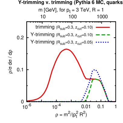
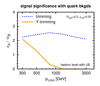
Figure 19: Comparisons of trimming and Y-trimming. Left: the $\rho$ distributions. Right: the signal significance for tagging $W$’s in the presence of quark backgrounds. The details of the MC event generation and cuts are as for Figs. 1 and 18 respectively.

References

- (1) A. Abdesselam, E. B. Kuutmann, U. Bitenc, G. Brooijmans, J. Butterworth, P. Bruckman de Renstrom, D. Buarque Franzosi and R. Buckingham et al., Eur. Phys. J. C 71 (2011) 1661 [arXiv:1012.5412 [hep-ph]].
- (2) A. Altheimer, S. Arora, L. Asquith, G. Brooijmans, J. Butterworth, M. Campanelli, B. Chapleau and A. E. Cholakian et al., J. Phys. G 39 (2012) 063001 [arXiv:1201.0008 [hep-ph]].
- (3) T. Plehn and M. Spannowsky, J. Phys. G 39 (2012) 083001 [arXiv:1112.4441 [hep-ph]].
- (4) G. Aad et al. [ATLAS Collaboration], JHEP 1205 (2012) 128 [arXiv:1203.4606 [hep-ex]].
- (5) G. Aad et al. [ATLAS Collaboration], Phys. Rev. D 86 (2012) 072006 [arXiv:1206.5369 [hep-ex]].
- (6) G. Aad et al. [ATLAS Collaboration], arXiv:1306.4945 [hep-ex].
- (7) S. Chatrchyan et al. [ CMS Collaboration], JHEP 1305 (2013) 090 [arXiv:1303.4811 [hep-ex]].
- (8) G. Aad et al. [ATLAS Collaboration], JHEP 1301 (2013) 116 [arXiv:1211.2202 [hep-ex]].
- (9) G. Aad et al. [ATLAS Collaboration], JHEP 1209 (2012) 041 [arXiv:1207.2409 [hep-ex]].
- (10) G. Aad et al. [ATLAS Collaboration], JHEP 1212 (2012) 086 [arXiv:1210.4813 [hep-ex]].
- (11) G. Aad et al. [ATLAS Collaboration], Eur. Phys. J. C 73 (2013) 2263 [arXiv:1210.4826 [hep-ex]].
- (12) S. Chatrchyan et al. [CMS Collaboration], JHEP 1209 (2012) 029 [arXiv:1204.2488 [hep-ex]].
- (13) S. Chatrchyan et al. [CMS Collaboration], JHEP 1212 (2012) 015 [arXiv:1209.4397 [hep-ex]].
- (14) S. Chatrchyan et al. [ CMS Collaboration], arXiv:1212.1910 [hep-ex].
- (15) G. Corcella, I. G. Knowles, G. Marchesini, S. Moretti, K. Odagiri, P. Richardson, M. H. Seymour and B. R. Webber, JHEP 0101 (2001) 010 [hep-ph/0011363].
- (16) M. Bahr, S. Gieseke, M. A. Gigg, D. Grellscheid, K. Hamilton, O. Latunde-Dada, S. Platzer and P. Richardson et al., Eur. Phys. J. C 58 (2008) 639 [arXiv:0803.0883 [hep-ph]].
- (17) T. Sjostrand, S. Mrenna and P. Z. Skands, JHEP 0605 (2006) 026 [hep-ph/0603175].
- (18) T. Sjostrand, S. Mrenna and P. Z. Skands, Comput. Phys. Commun. 178 (2008) 852 [arXiv:0710.3820 [hep-ph]].
- (19) T. Gleisberg, S. .Hoeche, F. Krauss, M. Schonherr, S. Schumann, F. Siegert and J. Winter, JHEP 0902 (2009) 007 [arXiv:0811.4622 [hep-ph]].
- (20) P. Richardson and D. Winn, Eur. Phys. J. C 72 (2012) 2178 [arXiv:1207.0380 [hep-ph]].
- (21) M. Rubin, JHEP 1005 (2010) 005 [arXiv:1002.4557 [hep-ph]].
- (22) M. Rubin, “A new LHC search channel for a light Higgs boson and associated QCD calculations,” Ph.D. Thesis, UPMC (University of Paris 6), 2010.
- (23) J. M. Butterworth, A. R. Davison, M. Rubin and G. P. Salam, Phys. Rev. Lett. 100 (2008) 242001 [arXiv:0802.2470 [hep-ph]].
- (24) J. R. Walsh and S. Zuberi, arXiv:1110.5333 [hep-ph].
- (25) I. Feige, M. D. Schwartz, I. W. Stewart and J. Thaler, Phys. Rev. Lett. 109 (2012) 092001 [arXiv:1204.3898 [hep-ph]].
- (26) J. Thaler and K. Van Tilburg, JHEP 1103 (2011) 015 [arXiv:1011.2268 [hep-ph]].
- (27) S. Catani, L. Trentadue, G. Turnock and B. R. Webber, Nucl. Phys. B 407 (1993) 3.
- (28) T. Becher and M. D. Schwartz, JHEP 0807 (2008) 034 [arXiv:0803.0342 [hep-ph]].
- (29) A. Gehrmann-De Ridder, T. Gehrmann, E. W. N. Glover and G. Heinrich, Phys. Rev. Lett. 99 (2007) 132002 [arXiv:0707.1285 [hep-ph]].
- (30) S. Weinzierl, Phys. Rev. Lett. 101 (2008) 162001 [arXiv:0807.3241 [hep-ph]].
- (31) M. Field, G. Gur-Ari, D. A. Kosower, L. Mannelli and G. Perez, arXiv:1212.2106 [hep-ph].
- (32) A. J. Larkoski, G. P. Salam and J. Thaler, arXiv:1305.0007 [hep-ph].
- (33) E. Gerwick, S. Schumann, B. Gripaios and B. Webber, JHEP 1304 (2013) 089 [arXiv:1212.5235 [hep-ph]].
- (34) P. Quiroga-Arias and S. Sapeta, arXiv:1209.2858 [hep-ph].
- (35) S. D. Ellis, C. K. Vermilion and J. R. Walsh, Phys. Rev. D 81 (2010) 094023 [arXiv:0912.0033 [hep-ph]].
- (36) S. D. Ellis, C. K. Vermilion and J. R. Walsh, Phys. Rev. D 80 (2009) 051501 [arXiv:0903.5081 [hep-ph]].
- (37) D. Krohn, J. Thaler and L. -T. Wang, JHEP 1002 (2010) 084 [arXiv:0912.1342 [hep-ph]].
- (38) T. Aaltonen et al. [CDF Collaboration], Phys. Rev. D 82 (2010) 034001 [arXiv:1003.3146 [hep-ex]].
- (39) Y. L. Dokshitzer, G. D. Leder, S. Moretti and B. R. Webber, JHEP 9708 (1997) 001 [hep-ph/9707323].
- (40) M. Wobisch and T. Wengler, In *Hamburg 1998/1999, Monte Carlo generators for HERA physics* 270-279 [hep-ph/9907280].
- (41) A. Katz, M. Son and B. Tweedie, JHEP 1103 (2011) 011 [arXiv:1010.5253 [hep-ph]].
- (42) M. Dasgupta, A. Fregoso, S. Marzani and A. Powling, arXiv:1307.0013 [hep-ph].
- (43) M. Dasgupta, L. Magnea and G. P. Salam, JHEP 0802 (2008) 055 [arXiv:0712.3014 [hep-ph]].
- (44) M. Dasgupta, K. Khelifa-Kerfa, S. Marzani and M. Spannowsky, JHEP 1210 (2012) 126 [arXiv:1207.1640 [hep-ph]].
- (45) B. Andersson, G. Gustafson, L. Lonnblad and U. Pettersson, Z. Phys. C 43 (1989) 625.
- (46) S. Catani, B. R. Webber and G. Marchesini, Nucl. Phys. B 349 (1991) 635.
- (47) M. Dasgupta and G. P. Salam, Phys. Lett. B 512 (2001) 323 [hep-ph/0104277].
- (48) R. B. Appleby and M. H. Seymour, JHEP 0212 (2002) 063 [hep-ph/0211426].
- (49) Y. Delenda, R. Appleby, M. Dasgupta and A. Banfi, JHEP 0612 (2006) 044 [hep-ph/0610242].
- (50) R. Kelley, J. R. Walsh and S. Zuberi, JHEP 1209 (2012) 117 [arXiv:1202.2361 [hep-ph]].
- (51) M. Cacciari, G. P. Salam and G. Soyez, JHEP 0804 (2008) 063 [arXiv:0802.1189 [hep-ph]].
- (52) M. Dasgupta and G. P. Salam, JHEP 0203 (2002) 017 [hep-ph/0203009].
- (53) A. Banfi, G. Marchesini, and G. Smye, JHEP 0208 (2002) 006 [hep-ph/0206076].
- (54) Y. Hatta and T. Ueda, Phys. Rev. D 80 (2009) 074018 [arXiv:0909.0056 [hep-ph]].
- (55) Y. Hatta and T. Ueda, arXiv:1304.6930 [hep-ph].
- (56) H. Weigert, Nucl. Phys. B 685 (2004) 321 [hep-ph/0312050].
- (57) J. R. Forshaw, A. Kyrieleis and M. H. Seymour, JHEP 0608 (2006) 059 [hep-ph/0604094].
- (58) Y. -T. Chien, R. Kelley, M. D. Schwartz, H. X. Zhu and , Phys. Rev. D 87 (2013) 014010 [arXiv:1208.0010 [hep-ph]].
- (59) T. T. Jouttenus, I. W. Stewart, F. J. Tackmann, W. J. Waalewijn and , arXiv:1302.0846 [hep-ph].
- (60) S. Catani, Y. L. Dokshitzer, M. Olsson, G. Turnock and B. R. Webber, “New clustering algorithm for multi - jet cross-sections in e+ e- annihilation,” Phys. Lett. B 269, 432 (1991);
- (61) S. Catani, Y. L. Dokshitzer, M. H. Seymour and B. R. Webber, “Longitudinally invariant K(t) clustering algorithms for hadron hadron collisions,” Nucl. Phys. B 406, 187 (1993).
- (62) Y. L. Dokshitzer, A. Lucenti, G. Marchesini and G. P. Salam, JHEP 9801 (1998) 011 [hep-ph/9801324].
- (63) J. M. Campbell, R. K. Ellis and , Phys. Rev. D 65 (2002) 113007 [hep-ph/0202176].
- (64) Z. Nagy, Phys. Rev. D 68 (2003) 094002 [hep-ph/0307268].
- (65) G. P. Korchemsky and G. F. Sterman, Nucl. Phys. B 437 (1995) 415 [hep-ph/9411211].
- (66) M. Dasgupta and Y. Delenda, JHEP 0907 (2009) 004 [arXiv:0903.2187 [hep-ph]].
- (67) G. P. Salam and D. Wicke, JHEP 0105 (2001) 061 [hep-ph/0102343].
- (68) V. Mateu, I. W. Stewart and J. Thaler, Phys. Rev. D 87 (2013) 014025 [arXiv:1209.3781 [hep-ph]].
- (69) A. D. Martin, W. J. Stirling, R. S. Thorne and G. Watt, Eur. Phys. J. C 63 (2009) 189 [arXiv:0901.0002 [hep-ph]].
- (70) T. Sjostrand and P. Z. Skands, Eur. Phys. J. C 39 (2005) 129 [hep-ph/0408302].
- (71) P. Z. Skands, Phys. Rev. D 82 (2010) 074018 [arXiv:1005.3457 [hep-ph]].
- (72) R. Corke and T. Sjostrand, JHEP 1103 (2011) 032 [arXiv:1011.1759 [hep-ph]].
- (73) G. Corcella, I. G. Knowles, G. Marchesini, S. Moretti, K. Odagiri, P. Richardson, M. H. Seymour and B. R. Webber, hep-ph/0210213.
- (74) K. Arnold, L. d’Errico, S. Gieseke, D. Grellscheid, K. Hamilton, A. Papaefstathiou, S. Platzer and P. Richardson et al., arXiv:1205.4902 [hep-ph].
- (75) L. Lonnblad, Comput. Phys. Commun. 118 (1999) 213 [hep-ph/9810208].
- (76) R. Field, arXiv:1010.3558 [hep-ph].
- (77) S. Frixione and B. R. Webber, JHEP 0206 (2002) 029 [hep-ph/0204244].
- (78) P. Nason, JHEP 0411 (2004) 040 [hep-ph/0409146].
- (79) S. Catani et al., JHEP 0111 (2001) 063 [arXiv:hep-ph/0109231].
- (80) J. Alwall et al., Eur. Phys. J. C 53 (2008) 473 [arXiv:0706.2569 [hep-ph]].
- (81) D. E. Soper and M. Spannowsky, JHEP 1008 (2010) 029 [arXiv:1005.0417 [hep-ph]].
- (82) Y. Cui, Z. Han and M. D. Schwartz, Phys. Rev. D 83 (2011) 074023 [arXiv:1012.2077 [hep-ph]].
- (83) J. Gallicchio and M. D. Schwartz, Phys. Rev. Lett. 105 (2010) 022001 [arXiv:1001.5027 [hep-ph]].
- (84) A. Hook, M. Jankowiak and J. G. Wacker, JHEP 1204 (2012) 007 [arXiv:1102.1012 [hep-ph]].
- (85) L. G. Almeida, S. J. Lee, G. Perez, G. Sterman and I. Sung, Phys. Rev. D 82 (2010) 054034 [arXiv:1006.2035 [hep-ph]].