pyro: A teaching code for computational astrophysical hydrodynamics

Abstract

We describe pyro: a simple, freely-available code to aid students in learning the computational hydrodynamics methods widely used in astrophysics. pyro is written with simplicity and learning in mind and intended to allow students to experiment with various methods popular in the field, including those for advection, compressible and incompressible hydrodynamics, multigrid, and diffusion in a finite-volume framework. We show some of the test problems from pyro, describe its design philosophy, and suggest extensions for students to build their understanding of these methods.

1 Introduction

The majority of the algorithms used for astrophysical fluid flow are first developed and described in journals devoted to applied math. Traditionally, astrophysics students are not exposed to these journals in their coursework, and their different target audience makes it difficult for a new astrophysics graduate student to come up to speed on the nuances of the methods. It is also the case that the potential audience of budding computational astrophysicist is sufficiently small in a graduate year that regular course offerings have trouble meeting the minimum class sizes imposed by a University. Often the goals of publicly-available production hydrodynamics codes, e.g. Flash (Fryxell et al., 2000) or Castro (Almgren et al., 2010), are not aligned with the needs of a teaching code. In particular, performance and breadth of options are favored over simplicity and clarity.

Our experience from working on as a developer number of different large simulation codes, including Flash (Fryxell et al., 2000), Castro, and Maestro (Nonaka et al., 2010) and with training students is that the best way to learn computational methods for hydrodynamics is to code them up yourself, or to make substantial modifications to the internals of existing code. For the latter, it helps to have a simple code as a starting point. Here we describe pyro (short for python hydro). pyro provides solvers for:

• linear advection

• compressible hydrodynamics

• elliptic PDEs via multigrid

• implicit diffusion

• incompressible hydrodynamics

All solvers are 2-d and second-order accurate in space and time. We chose 2-d because some of the key design issues in writing a solver are not present in the simpler 1-d algorithms. Furthermore, 2-d offers sufficient complexity that the transition to 3-d is then straightforward for a student. Finally, 2-d allows for an exploration of grid effects and instabilities in the solver that 1-d does not allow. pyro is intended for self-study. An accompanying set of detailed lecture notes help explain the core methods and experimentation is encouraged. These notes have been used by undergraduate researchers working with the author and are continually refined based on these interactions.

While there is a large variety of different methods for each of these systems of equations, we pick a single method representative of those used in astrophysics and implement it. Given the choice between clarity and performance, we take clarity. Variations and enhancements are left as exercises for students.

There are a number of excellent books that explain the basic theory of numerical solution of PDEs, like LeVeque (2002) for finite-volume methods and Briggs et al. (2000) for multigrid, but students also need hands-on experience, to experiment, break, and tweak the algorithms. Little details, like the number of ghost cells needed for different parts of the algorithm are often not obvious to new students, so a basic starting platform from which they can build on provides a good introduction. pyro is written to help fill this need. pyro is freely-available at https://github.com/zingale/pyro2 with documentation provided at http://bender.astro.sunysb.edu/hydro_by_example/

The core algorithms implemented in pyro are not new—the new part of pyro is the focus on teaching the methods to the next generation of students through a clean, robust implementation and hands-on activities. The purpose of this paper is to give an overview of the algorithms pyro provides, show some results from the various test problems, demonstrating the validity of the methods we implement, and provide ideas for extensions to help new students to the field build their understanding. This paper is complemented by detailed notes describing the derivation and implementation of the various methods, available on the pyro website, and, of course, the freely-available source code itself.

2 Design

Python provides an attractive platform for quickly testing out different ideas. It is easy to use, freely-available, and with the NumPy package, a powerful language for manipulating arrays of data. However, being an interpreted language, the best performance is attained when you allow NumPy to work on entire arrays of data instead of explicitly looping over the individual elements. There are some instances when the NumPy array notation can look cumbersome, and hide from simple inspection the differencing being done. For example, consider constructing a second-derivative as:

$$a^{\prime\prime}_{i}=\frac{a_{i+1}-2a_{i}+a_{i-1}}{\Delta x^{2}}$$ (1)

Here the subscripts represent the index into a sequence of regularly gridded data. If we have a NumPy array a, with appropriate ghost cells, and use the integers lo and hi to refer to the first and last valid cells, then we can write this in slice-notation as:

d2a_dx2[lo:hi+1] = a[lo+1:hi+2] - \
               2.0*a[lo  :hi+1] + \
                   a[lo-1:hi]
d2a_dx2[:] = d2a_dx2[:]/dx**2

This is efficient in python, but makes the underlying index notation we are used to seeing in papers hidden (especially in 2-d). For more complex constructions, with nonlinear switches (e.g. if conditions), the NumPy form can be complex. To strike the right balance in terms of clarity and use of NumPy’s advanced features, we implement some kernels in Fortran, using f2py to interface with python. Wherever Fortran is used, we enforce the following design rule: the Fortran functions must be completely self-contained, with all information coming through the interface. No external dependencies are allowed. Each pyro module will have (at most) a single Fortran file and can be compiled into a library via a single f2py command line invocation.

There are two fundamental classes in pyro that manage the data. The Grid2d class describes the grid, providing the basic coordinate information and the CellCenterData2d class describes the data that lives on the grid. Building a CellCenterData2d object takes a Grid2d object at initialization and has methods to register variables that live on the grid. Each variable can have its own boundary condition types and methods exist for getting access to a single variable, filling ghost cells, restricting and prolonging a data to a new grid (used by the multigrid solver), printing data to the screen (useful only for small grids), and writing the data to disk.

Each solver is given its own directory, with problems/ and tests/ sub-directories. The former holds the initial condition routines and default parameters for each of the problems known to that solver. The latter stores benchmark output and is used for the built-in regression testing.

solver	problem	problem description
advection	smooth	advect a smooth Gaussian profile
	tophat	advect a discontinuous tophat profile
compressible	bubble	a buoyant bubble in a stratified atmosphere
	kh	setup a shear layer to drive Kelvin-Helmholtz instabilities
	quad	2-d Riemann problem based on Schulz-Rinne et al. (1993)
	rt	a simple Rayleigh-Taylor instability
	sedov	the classic Sedov-Taylor blast wave
	sod	the Sod shock tube problem
diffusion	gaussian	diffuse an initial Gaussian profile
incompressible	converge	A simple incompressible problem with known analytic solution.
	shear	a doubly-periodic shear layer

Table 1: Solvers and their distributed problems

One of the concepts that comes out of the code is how similar the solution methodology is for the different PDE systems. The grid requirements/data locations are the same, the boundary conditions types are analogous, and even the overall flowchart of the main driver is the same. For all time-dependent solvers (i.e., excepting multigrid) the basic flowchart is:

• parse runtime parameters

• setup the grid

• set the initial conditions for the data on the grid

• do any necessary pre-evolution initialization

• evolve while $t<\mathtt{tmax}$ or $n<\mathtt{max\_steps}$:

  • fill boundary conditions

  • get the timestep

  • evolve for a single timestep

  • t = t + dt;  n = n + 1

  • output

  • visualization

This allows us to have a single driver for all the solvers. pyro is run as:

./pyro.py [options] solver problem infile [runtime-options]

where solver is one of advection, compressible, diffusion, or incompressible. The problem gives the name of the problem whose initial conditions we use—these vary by solver (see Table 1). Finally the infile overrides any default runtime parameters for the run. Runtime parameters are defined both in the main pyro directory and for each solver and problem in plain text files that are parsed at runtime. Optionally, runtime parameters defaults can also be overridden at the end of the commandline. The collection of runtime parameters is managed by the RuntimeParameters class.

The interaction with the different solvers is done through each solver’s Simulation class which holds the simulation’s RuntimeParameters object, the CellCenterData2d data, and some timer information (for profiling). The class provides the following methods:

• initialize(): set up the grid and solution variables.

• timestep(): return the timestep for evolving the system.

• preevolve(): do any initialization to the fluid state that is necessary before the main evolution. Not every solver will need something here.

• evolve(): advance the system of equations through a single timestep.

• dovis(): perform visualization of the current solution.

• finalize(): any final clean-ups, printing of analysis hints.

I/O is done simply using the python pickle module on the main data object. Finally, by default, runtime visualization is enabled using the matplotlib plotting library. The output is updated each timestep to allow students to see the progression of their simulations as they run. This is very useful for seeing the effects of boundary conditions and different choices of initial conditions as well as for chasing down bugs.

2.1 Software engineering ideas

Astronomy students benefit from learning basic “safe practices” from software engineering (Ferland, 2002; Wilson et al., 2012; Turk, 2013). pyro facilitates this in three ways. First, pyro is open source, released under a BSD-3 license. Sharing of code helps find bugs, as more eyes are now on the source. Furthermore, open code is increasingly being seen as part of the scientific peer-review proces (Shamir et al., 2013).

Secondly, support for regression testing is built into pyro. In its simplest form, regression testing means comparing the current solution to a known benchmark solution, and looking for differences. When pyro is run with the --make_benchmark option, it will automatically store a benchmark solution for the problem in the solver’s tests/ sub-directory. When run with the --compare_benchmark option, the current results will be compared zone-by-zone with the stored benchmark, and any differences will be reported. We note that comparing bit-for-bit in each zone means that we may not find agreement when comparing across different platforms because of floating point differences. An alternative is check for agreement in each zone to within some tolerance. Both approaches have value. We prefer the exact comparison and it is what is used in the regression suites for the production codes we have worked with—e.g., this is done by the sfocu comparison tool in the flashTest regression framework (Flash Center for Computational Science, 2014). If there is some round-off level difference in output, checking to within a tolerance may not catch it, but the exact comparison will. The developer can then check to see if a code change is responsible for floating point differences or whether some underlying change to the software enviroment is at play. In either scenario, the developer is made aware of a difference in the output that comparison to within some tolerance would miss. The downside is that unique benchmarks may need to be made on each platform.

Finally, as is increasingly the case in astrophysics (see e.g. the Castro code or yt Turk et al. 2011) it is obtained via a distributed version control system (git in our case, recently migrated to GitHub), immediately immersing students in version control—each student’s clone of the pyro repo acts as its own git repo that they can interact with directly. We have taught several graduate classes where a basic introduction to programming practices was given, and we found that many students were simply unaware of the idea of version control. Once the concept was introduced, we have seen many students start to use it for their own projects.

3 Algorithm Summaries and Tests

Here we give an overview of the methods pyro implements and show some verification tests.

When solving a system of PDEs, continuous derivatives are replaced by their discretized counterparts, either by making reference to an underlying grid, or by using a collection of particles to represent the functional distribution. Within astrophysics, both grid base and particle-base methods are popular, and each has their own strengths and weaknesses (see e.g. Agertz et al. 2007; Hubber et al. 2013 and references therein). We focus here on structured grids—logically Cartesian grids where any zone can be references by a single integer in each dimension. Structured grids are popular because the geometries of our domains are generally not complex, and because structured grids can make good use of modern cache-based architectures. Both finite-difference and finite-volume methods are structured-grid discretizations popular in astrophysics. A finite-volume method represents the data as an average within a volume (or zone) while a finite-difference grid stores the function value at a specific point. These differences arise from whether we choose to work with the integral form (finite-volume) or differential form (finite-difference) of our system of equations. We note that a cell-centered finite-difference grid is equivalent to a finite-volume grid to second-order in $\Delta x$. We choose the finite-volume grid here, and use the convention that zone centers are indicated by an integer, $i$, while the interfaces are marked by a half-integer ($i-1/2$ on the left and $i+1/2$ on the right). Figure 1 illustrates the grid in 1-d.

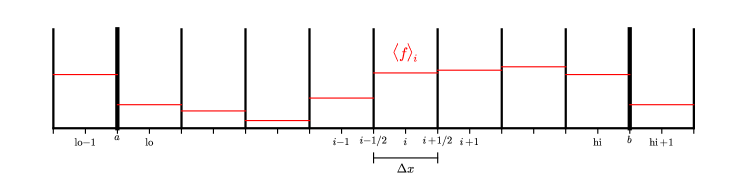
Figure 1: A (1-d) finite-volume grid. The domain boundaries are indicated by the thick lines and a single ghost cell is shown. $\mathrm{lo}$ and $\mathrm{hi}$ indicate the first and last valid cells. $a$ and $b$ mark the locations of the left and right boundaries.

3.1 Advection

The linear advection equation represents the simplest hyperbolic PDE:

$$a_{t}+ua_{x}+va_{y}=0$$ (2)

The solution is trivial—any initial function profile simply advects unchanged with a velocity $u\hat{x}+v\hat{y}$. This makes advection an excellent test bed of numerical methods.

Advection also provides a good path toward understanding how to extend to multi-dimensions. There are two approaches here: dimensional splitting and unsplit reconstruction. In dimensional splitting, the fluxes at the interfaces are constructed without any knowledge of the flow in the transverse direction. Each directional update operates on the state left behind by the previous update and the order of directions is alternated to give second-order accuracy (Strang, 1968). This is the easiest way to extend from one-dimension to multi-dimensions, because you can use the 1-d methodology largely unchanged. However, split methods do not preserve symmetries as well (see, e.g. Almgren et al. 2010). In an unsplit reconstruction, each interface state explicitly sees the change carried in the transverse direction, and the state is updated by the fluxes in each direction all at once.

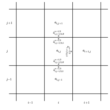
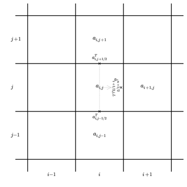
Figure 2: The construction of the $a_{i+1/2,j,L}^{n+1/2}$ state. Left: first we compute the $\hat{a}$’s—here we show all of the $\hat{a}$’s that will be used in computing the full left interface state at $(i+1/2,j)$. Right: after the transverse Riemann solves, we have the two transverse states ($a^{T}_{i,j+1/2}$ and $a^{T}_{i,j-1/2}$) that will be differenced and used to correct $\hat{a}_{i+1/2,j,L}^{n+1/2}$ (illustrated by the dotted lines) to make $a_{i+1/2,j,L}^{n+1/2}$.

We follow the unsplit CTU method (Colella, 1990) for advection. We summarize this method in a little detail below because the same procedure comes into play again for our compressible and incompressible solvers. The basic idea is simple—Taylor expand in space and time to get the time-centered interface state and use this to evaluate the fluxes through the interfaces. For example, the left state at the $i+1/2,j$ interface is built starting with the data in cell $i,j$ as

$$a_{i+1/2,j,L}^{n+1/2}=a_{i,j}^{n}+\frac{1}{2}\left(1-\frac{\Delta t}{\Delta x}u\right)\left.\overline{\Delta a}\right|_{i,j}-\frac{\Delta t}{2}v\left.\frac{\partial a}{\partial y}\right|_{i,j}$$ (3)

The last term here is the transverse flux difference and captures the change in $a$ in the transverse direction. Without this term, if we advect diagonally, we would not ‘see’ the upwind state. The $\overline{\Delta a}$ term is the limited slope of $a$—limiting ensures that we don’t have any over- or under-shoots when we advect (although see Bell et al. (1988) for details about limiting in multi-dimensions). A number of different choices of limiters are described in the literature. We use the 4th-order MC limiter from Colella (1985). We rewrite this as:

$$a_{i+1/2,j,L}^{n+1/2}=\hat{a}_{i+1/2,j,L}^{n+1/2}-\frac{\Delta t}{2}v\left.\frac{\partial a}{\partial y}\right|_{i,j}$$ (4)

where the $\hat{a}_{i+1/2,j,L}^{n+1/2}$ state represents the prediction to the interface without regard to the transverse term. The basic idea of the CTU method is to first construct these ‘hat’ states on all interfaces, then solve the Riemann problem at each interface to find the ‘transverse’ state, $a^{T}_{i+1/2,j}$—this is the unique state on each interface. So far however, we did not consider the transverse term in Eq. 3. This transverse term is constructed using the $a^{T}$ edge states and added to the $\hat{a}$ states giving us the full interface state $a_{i+1/2,j,L}^{n+1/2}$. This is illustrated graphically in Figure 2.

A similar reconstruction gives the predicted state just to the right of the interface, $a_{i+1/2,j,R}^{n+1/2}$, building from the data in the $i+1,j$ cell. The final state on the interface, $a_{i+1/2,j}^{n+1/2}$ is attained by calling the Riemann solver again. For advection, the Riemann solve is simply upwinding, but for other systems it is more complex. The states in the $y$-direction are computed analogously. This then allows us to increment our solution:

$$\frac{a_{i,j}^{n+1}-a_{i,j}^{n}}{\Delta t}= -\frac{(ua)_{i+1/2,j}^{n+1/2}-(ua)_{i-1/2,j}^{n+1/2}}{\Delta x}$$

$$-\frac{(va)_{i,j+1/2}^{n+1/2}-(va)_{i,j-1/2}^{n+1/2}}{\Delta y}$$ (5)

The timestep constraint is simply

$$\Delta t=C\min\left\{\frac{\Delta x}{u},\frac{\Delta y}{v}\right\}$$ (6)

where $C\leq 1$ is the CFL number.

3.1.1 Smooth advection test

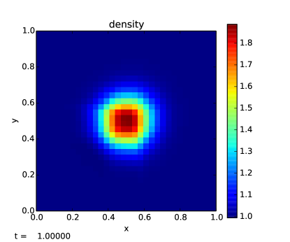
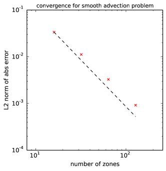
Figure 3: Linear advection of a Gaussian profile. Left shows the profile on a $32^{2}$ grid after advecting diagonally for a period. Right shows the convergence of the solver, with the dotted line representing $\mathcal{O}(\Delta x^{2})$ scaling. This example was run with: ./pyro.py advection smooth inputs.smooth. The different resolutions were run by changing mesh.nx and mesh.ny. The errors for the plot on the right were computed with analysis/smooth_error.py.

The simplest test is to advect a smooth distribution diagonally across our grid for one period. Since the profile should be unchanged, we can define the error simply as the difference between the final and initial profile, and look at the norm of the error to assess the convergence. A smooth problem is chosen so as to reduce the effects of the limiters—we choose a Gaussian:

$$a(x,y)=1+e^{-A[(x-x_{c})^{2}+(y-y_{c})^{2}]}$$ (7)

where $(x_{c},y_{c})$ are the coordinates of the center of the domain and $A$ is a width parameter. We choose $A=60$. Figure 3 shows the solution after 1 period with $u=v=1$, a CFL number of 0.8, and for one resolution ($32^{2}$) along with a convergence plot of the error as a function of resolution, showing that we are nearly second-order accurate. The departure from perfect second-order convergence arises from the use of limiters.

3.1.2 Explorations for students

With this basic solver, there are a number of exercises/extensions that students can perform to improve their understanding:

• Compare convergence with limiting to no limiting.

• How does the solution change if the transverse flux difference is left out?

• Implement a dimensionally split version and compare to the unsplit.

• Convert the solver to the inviscid Burger’s equation ($u_{t}+uu_{x}=0$) and look at shocks and rarefactions.

3.2 Compressible hydrodynamics

Compressible hydrodynamics is described by the Euler equations:

$$\rho_{t}+\nabla\cdot(\rho U) = 0$$ (8)

$$(\rho U)_{t}+\nabla\cdot(\rho UU)+\nabla p = \rho g$$ (9)

$$(\rho E)_{t}+\nabla\cdot(\rho UE+Up) = \rho U\cdot g$$ (10)

Here, $\rho$ is the density, $U$ is the velocity vector, $p$ is the pressure, and $E$ is the total specific energy, related to the specific internal energy, $e$, via

$$E=e+\frac{1}{2}U^{2}$$ (11)

We include a gravitational source, with $g$ the constant gravitational acceleration. We need an equation of state to close the system. We assume a gamma-law:

$$p=\rho e(\gamma-1)$$ (12)

The solution procedure we adopt is the unsplit piecewise-linear method described in Colella (1990). This same algorithm is also one of the hydrodynamics options in the Castro code (Almgren et al., 2010). While formally less accurate than the widely-used piecewise parabolic method, PPM (Colella and Woodward, 1984), piecewise linear reconstruction is more approachable for new students, and upgrading to PPM is straightforward once the details are understood (see Miller and Colella 2002 for a good discussion).

The algorithm follows the advection update closely. Again, interface states are constructed by doing a Taylor expansion to the half-time, interface state. Now however, the normal part of the prediction is done in terms of the primitive variables, $q=(\rho,u,v,p)^{\intercal}$, instead of the conserved variables. A characteristic projection is done on the state and only the jumps moving toward the interface are added to the interface state. These preliminary interface states are converted back to the conserved variables and the transverse flux difference is added. An initial construction of the normal interface states is used to construct the fluxes for the transverse difference. Our implementation follows Colella (1990). We also include the flattening of the profiles near shocks and artificial viscosity from that paper.

One confusing aspect of these methods for new students is the characteristic projection. Writing the primitive variable system as $q_{t}+Aq_{x}=0$, the jump in a primitive variable, $\Delta q$ can be expressed in terms of the left and right eigenvectors, $l$ and $r$ of $A$ as:

$$\Delta q=\sum_{\nu}(l^{(\nu)}\cdot\Delta q)r^{(\nu)}$$ (13)

LeVeque (2002) provides an excellent introduction to this concept. Typically in this sum, we only include the terms where the waves are moving toward the interface of interest (determined by the sign of the eigenvalues). Most papers write only the analytic result of multiplying out $(l^{(\nu)}\cdot\Delta q)$ (e.g. see the $\beta$’s in Eqs. 3.6, 3.7 in Colella and Woodward 1984). For clarity, and to enable exploration, in pyro, we explicitly construct the left and right eigenvectors and multiply them through in the code, to illustrate exactly what the solution procedure is doing.

The Riemann problem for compressible hydrodynamics is considerably more complex than linear advection. There are 3 waves that result from the system (corresponding to the $u-c$, $u$, and $u+c$ eigenvalues of $A$), and each wave, $\nu$, carries a jump in the state proportional to $r^{(\nu)}$. The solution to the Riemann problem looks at wave structure to determine the solution in-between the various waves and evaluates the wavespeeds to determine which state is on the interface. This state is then used to construct the fluxes through the interface. Because of the expense of the full Riemann solve, approximate Riemann solvers are often used. We use the Riemann solver described in Almgren et al. (2010), and alternately the HLLC method from Toro (1997).

3.2.1 Sod shock tube

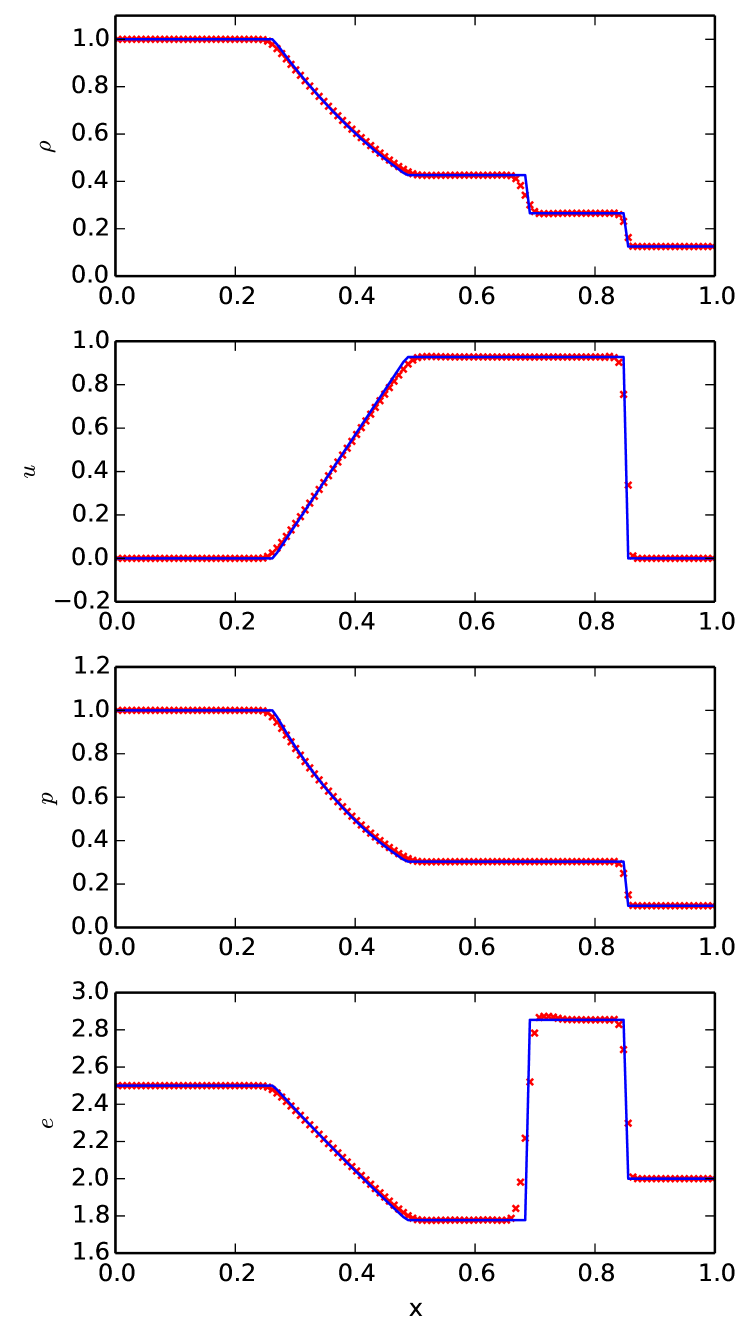
Figure 4: Sod problem with 128 zones compared to the exact solution at t = 0.2. We show a slice through the center of the domain along $x$. This example was run with: ./pyro.py compressible sod inputs.sod.x , and the comparison to the analytic data was done with analysis/sod_compare.py.

The Sod shock tube (Sod, 1978) illustrates all three types of hydrodynamic waves: a rarefaction, contact, and shock wave. This problem is a standard test of hydrodynamics solvers because exact solutions are possible. We compare to the result from the exact Riemann solver in Toro (1997).

Figure 4 shows the results from a simulation on a $128\times 10$ grid with the initial discontinuity in the $x$-direction. The CFL number was 0.8 and $\gamma=1.4$. The shock is very steep, the contact is smeared out a bit (there is no self-steepening mechanism for contacts, so this is commonly seen). Overall the solution matches the analytic profile well. The discontinuities in the solution mean that taking the norm of the error with the exact solution has little value.

3.2.2 Sedov-Taylor blast wave

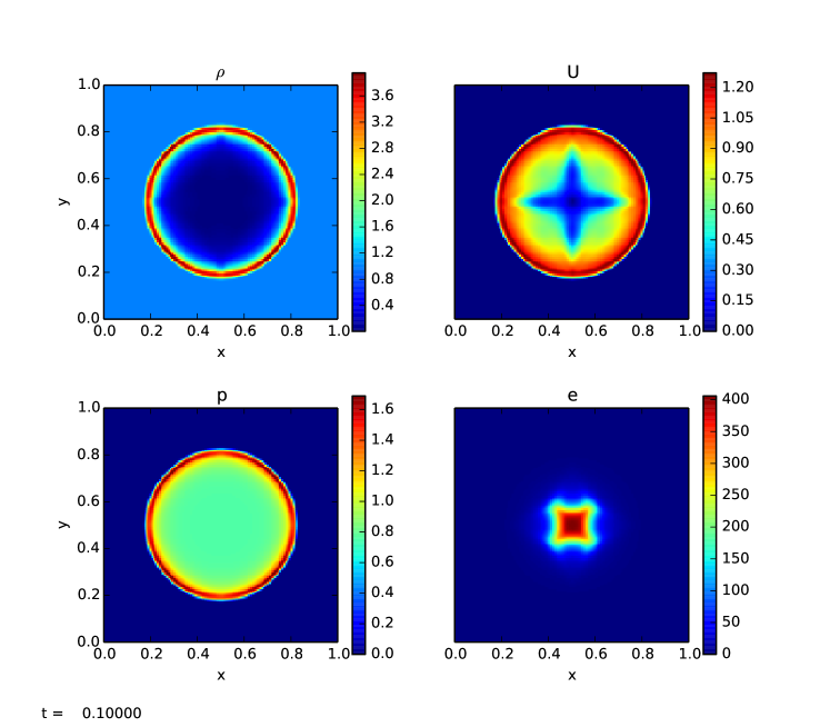
Figure 5: Solution to the Sedov problem at $t=0.1$. This example was run with: ./pyro.py compressible sedov inputs.sedov

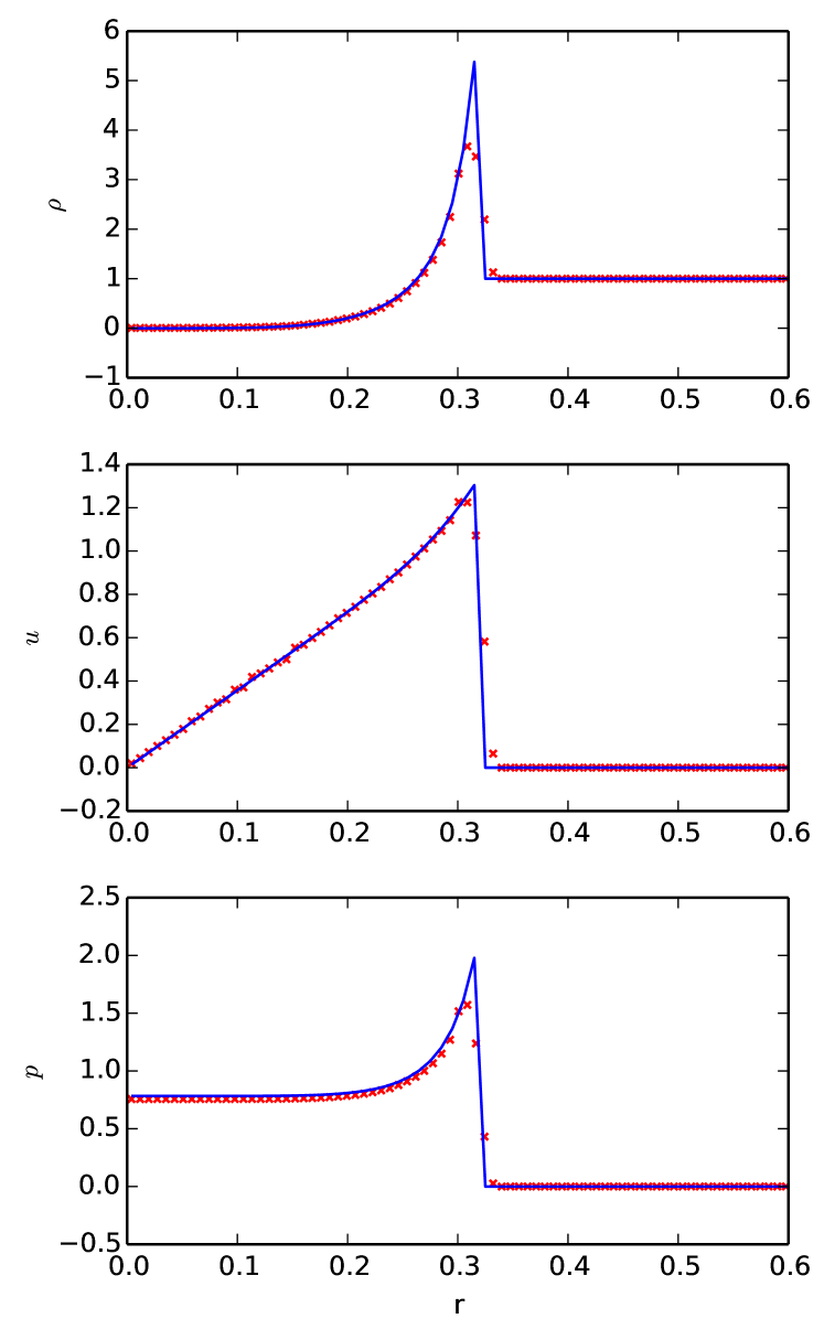
Figure 6: Angle-averaged profiles for the Sedov problem for a $128^{2}$ simulation at $t=0.1$. The solid line is the exact solution. This figure was created with the analysis/sedov_compare.py script.

The Sedov-Taylor blast wave is a good test of the symmetry-preservation of the method. A large amount of energy, $\mathcal{E}$, is placed at a point in a uniform medium. The blast wave should stay circular (in 2-d), with the density evacuating and the pressure reaching a constant at the center. An analytic solution was worked out for this problem (Sedov, 1959). A good description of the solution is given in Kamm and Timmes (2007)—we compare to the solution from that paper.

A difficulty with the Sedov problem on a 2-d Cartesian grid is that the point that the energy is deposited to will be square on the grid, leading to some grid effects. We take the standard approach of converting the energy into a pressure contained in a circular region:

$$p=(\gamma-1)\frac{\mathcal{E}}{\pi r_{\mathrm{init}}^{2}}$$ (14)

To further reduce grid effects, we sub-divide each zone into $4^{2}$ sub-zones and test whether each sub-zone falls inside the perturbed radius, and average over the sub-zones to get a single pressure for the zone. We choose $\mathcal{E}=1.0$, $r_{\mathrm{init}}=0.01$, and $\gamma=1.4$. We run on a $128^{2}$ grid with a CFL number of 0.8. Figure 5 shows the various fluid quantities. We see a nice circular blast wave, but some grid effects are seen aligned with the coordinate axes. The angle-averaged data (profiles as a function of radius) are shown in Figure 6. We see very good agreement with the exact solution.

3.2.3 Rayleigh-Taylor instability

The Rayleigh-Taylor instability places a dense fluid over a lighter fluid in a gravitational field. Given an initial perturbation, the dense fluid drops down and the lighter fluid buoyantly rises upward. Our initial conditions are:

$$\rho=\left\{\begin{array}[]{cc}\rho_{1}&\mathrm{if~{}}y<y_{c}\\ \rho_{2}&\mathrm{if~{}}y\geq y_{c}\end{array}\right.$$ (15)

The pressure is given by hydrostatic equilibrium, which for constant $g$ integrates easily giving:

$$p=\left\{\begin{array}[]{cc}p_{0}+\rho_{1}gy&\mathrm{if~{}}y<y_{c}\\ p_{0}+\rho_{1}gy_{c}+\rho_{2}g(y-y_{c})&\mathrm{if~{}}y\geq y_{c}\end{array}\right.$$ (16)

The perturbation is given in the $y$-velocity:

$$v=A\cos(2\pi x/L_{x})*e^{-(y-y_{c})^{2}/\sigma^{2}}$$ (17)

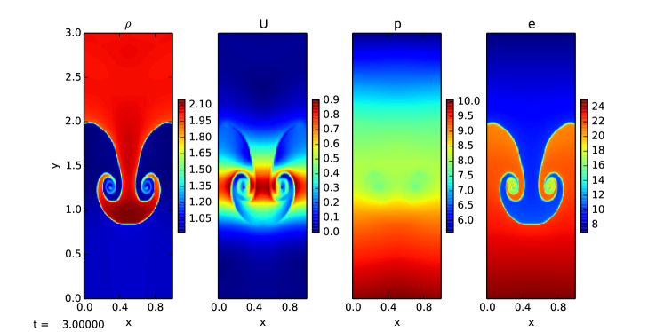
Figure 7: A single-mode Rayleigh-Taylor instability calculation with a 2:1 density ratio at $t=3.0$. This was run with ./pyro.py compressible rt inputs.rt

Periodic boundary conditions are used in the horizontal direction. We use hydrostatic boundary conditions in the vertical direction. This is one example of where the treatment of the boundary is solver-dependent, so the compressible solver provides a method that is called from the main mesh module to extend the functionality of the boundary filling. For this boundary condition, the density and $x$- and $y$-momenta are simply copied from the last valid zone inside the domain (a zero-gradient). The energy is filled in the ghost cells by first constructing the pressure in the zone just inside the boundary and then using hydrostatic equilibrium to integrate this pressure into the ghost cells. Since the density and gravity are constant, this integration is trivial. This pressure is then used to construct the total energy in the ghost cells. This method is similar to that from Zingale et al. (2002).

Figure 7 shows the results for a $128\times 384$ zone grid with a CFL of 0.8. We see that this single mode RT is very symmetric, and in good agreement with the results shown in Almgren et al. (2010).

3.2.4 Explorations for students

After understanding the basic algorithm, there are a number of extensions that can be done to build a deeper understanding of the method.

• Compare the solutions with and without limiting.

• Limit on the characteristic variables instead of the primitive variables (see Stone et al. 2008).

• Add passively advected species to the solver.

• Add an external heating term to the equations.

• Add 2-d axisymmetric coordinates (r-z) to the solver.

• Swap the piecewise linear reconstruction for piecewise parabolic (PPM).

• Add different Riemann solvers to the algorithm.

3.3 Multigrid

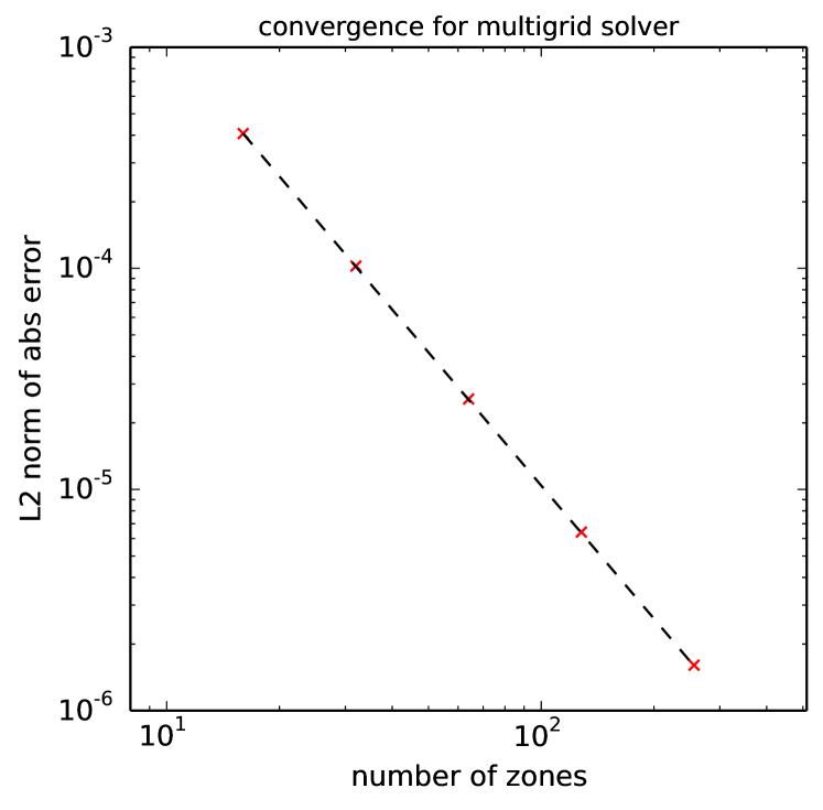
Figure 8: L2 norm of the error for the multigrid test problem, showing second-order accuracy. This example was run at several resolutions using the mg_test.py script in the multigrid module—that script reports the error at the end of execution.

Multigrid is a popular technique for solving elliptic problems in simulation codes (a widely-used example is the Poisson problem for the gravitational potential). The pyro multigrid solver solves a constant-coefficient Helmholtz equation of the form:

$$(\alpha-\beta\nabla^{2})\phi=f$$ (18)

The choice $(\alpha,\beta)=(0,-1)$ gives the classic Poisson equation.

The text of Briggs et al. (2000) provides an excellent introduction to multigrid techniques. Most of it, however, is geared toward finite-difference grids, where solution values exist explicitly on the boundary. For cell-centered/finite-volume grids (see Figure 1), the implementation of the restriction and prolongation operations differs, as does the enforcement of the boundary conditions. In fact, boundary conditions for cell-centered grids is probably the most common place that mistakes are made. A good way to test this all is to get pure relaxation working first, and converging to second-order. Multigrid simply accelerates the convergence of the relaxation, so if the relaxation routine is not right, then there is no point going further. pyro provides an easy test bed for experimenting with these ideas.

To make the code simple, we restrict ourselves to pure V-cycles and solve on square domains with the number of zones a power of 2. Red-black Gauss-Seidel relaxation is done. The restriction operation is simply averaging the four fine cells into the corresponding coarse cell. For prolongation, we create centered-slopes in each direction centered for every coarse cell and use a bilinear interpolation (without the cross $xy$ term) to fill each of the four finer cells. Furthermore, we only support homogeneous Dirichlet or Neumann boundary conditions. The grid is coarsened until we get down to a $2^{2}$ grid, at which point the residual equation is solved by pure relaxation, doing, by default, 50 smoothing iterations on the $2^{2}$ grid.

For homogeneous Dirichlet boundary conditions, the goal is to have the solution be 0 exactly at the interface of the zone touching the domain boundary. Consider the left boundary (see Figure 1): we want $\phi_{a}=0$. The standard approach (to second-order accuracy) is to average the adjacent cells to that interface, and set this to zero, giving:

$$\phi_{\mathrm{lo}-1,j}=-\phi_{\mathrm{lo},j}$$ (19)

A similar construction is done at the upper boundary in $x$, and for the boundaries in $y$. Neumann BCs are done in a similar fashion—we construct a difference that is centered at the interface, so to second-order, we have

$$\phi_{\mathrm{lo}-1,j}=\phi_{\mathrm{lo},j}$$ (20)

Inhomogeneous boundary conditions would be treated similarly, but now the boundary value itself will appear in the expression for the ghost cell.

3.3.1 Poisson-solve test problem

To test the multigrid solver, we solve a Poisson problem with a known analytic solution. This example comes from Briggs et al. (2000):

$$\nabla^{2}\phi=-2\bigl{[} (1-6x^{2})y^{2}(1-y^{2})+$$

$$(1-6y^{2})x^{2}(1-x^{2})\bigr{]}$$ (21)

solved on a unit square with $\phi=0$ on the boundary. The analytic solution in this case is:

$$\phi(x,y)=(x^{2}-x^{4})(y^{4}-y^{2})$$ (22)

We continue to cycle until the relative error (L2 norm of the residual / L2 norm of the source) is less than $10^{-11}$. Figure 8 shows L2-norm of the absolute error of our solution compared to the analytic solution for a variety of resolutions. We see perfect second-order convergence.

3.3.2 Explorations for students

• Instead of doing multigrid, run with smoothing only and look at how long it takes to converge.

• Implement inhomogeneous BCs.

• Experiment with different bottom solvers.

3.4 Implicit diffusion

Many phenomena can be described by the diffusion equation:

$$\phi_{t}=k\phi_{xx}$$ (23)

including thermal diffusion/conduction and viscosity. Here, $k$ is the diffusion coefficient, which we will take to be constant, and $\phi$ is the scalar quantity being diffused. The diffusion solver uses multigrid to solve an implicit Crank-Nicolson (centered in time) discretization of the diffusion equation:

$$\frac{\phi^{n+1}_{i}-\phi^{n}_{i}}{\Delta t}=\frac{1}{2}\left(k\nabla^{2}\phi^{n}_{i}+k\nabla^{2}\phi^{n+1}_{i}\right)$$ (24)

Grouping all the $n+1$ terms on the left, we find:

$$\phi^{n+1}_{i}-\frac{\Delta t}{2}k\nabla^{2}\phi^{n+1}_{i}=\phi^{n}_{i}+\frac{\Delta t}{2}k\nabla^{2}\phi^{n}_{i}$$ (25)

This is in the form of a constant-coefficient Helmholtz equation, Eq. 18, with

$$\alpha=1,\,\,\beta=\frac{\Delta t}{2}k,\,\,f=\phi^{n}+\frac{\Delta t}{2}k\nabla^{2}\phi^{n}$$ (26)

An update over a single timestep is achieved by simply calling the multigrid solver. Since this solver is implicit, there is no timestep limit for stability, but accuracy will of course be better with a smaller timestep. For this solver, the CFL number in the driver, $C$, is based on the explicit timestep limit:

$$\Delta t=C\frac{\Delta x^{2}}{k}$$ (27)

where $C\leq 1/2$ is needed for a standard explicit discretization of the diffusion equation.

3.4.1 Diffusion of a Gaussian test problem

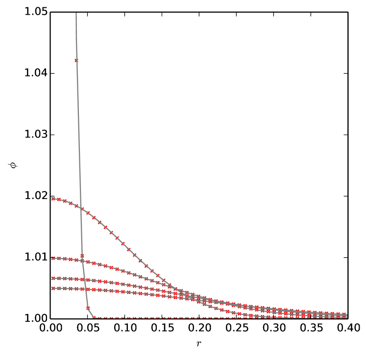
Figure 9: Radial profile of the diffusion of a Gaussian shown every $\Delta t=0.005$ starting with $t=0$, using $C=2.0$ and a $128^{2}$ grid. The analytic solution is shown as the gray line. We see excellent agreement. This example was run with: ./pyro.py diffusion gaussian inputs.gaussian, and the comparison with the analytic solution was done with the analysis/gauss_diffusion_compare.py script.

An initial Gaussian profile remains a Gaussian under the action of diffusion, with the amplitude decreasing and width increasing. This allows us to test the diffusion solver against the analytic solution (see, e.g. Swesty and Myra 2009):

$$\phi(x,t)=(\phi_{2}-\phi_{1}){\frac{t_{0}}{t+t_{0}}}e^{-\frac{1}{4}[(x-x_{c})^{2}+(y-y_{c})^{2}]/k(t+t_{0})}+\phi_{1}$$ (28)

For the initial conditions, we take $t_{0}=0.0001$, $\phi_{1}=1$, and $\phi_{2}=2$. We run with $k=1$. Figure 9 shows the angle-averaged radial profile at several different times together with the analytic solution for a run on a $128^{2}$ grid with $C=2.0$. We see excellent agreement.

3.4.2 Exercises for students

There are a number of straightforward exercises and extensions

• Experiment with different-sized timesteps and initially discontinuous data.

• Implement a non-constant diffusion coefficient solver.

• Compare Crank-Nicolson to backwards Euler.

3.5 Incompressible Hydrodynamics

The equations of incompressible flow are:

$$U_{t}+U\cdot\nabla U+\nabla p =0$$ (29)

$$\nabla\cdot U =0$$ (30)

Incompressible flow adds a additional complexity to our systems—now an elliptic constraint is present on the velocity field that must also be satisfied at each timestep. It is also an important stepping-stone toward understanding low Mach number methods, used for both smallscale combustion (Bell et al., 2004) and stratified flows (Nonaka et al., 2010).

pyro’s incompressible solver follows a second-order projection methodology (see, Chorin 1968; Bell et al. 1989). A projection method relies on the fact that any vector field, $U^{\star}$ can be decomposed into a divergence-free part, $U^{d}$, and the gradient of a scalar:

$$U^{\star}=U^{d}+\nabla\phi$$ (31)

The idea is that we first use the same unsplit advection techniques as with linear advection and compressible flow to update $U$ to the new time, giving a velocity field $U^{\star}$ that does not yet satisfy the divergence constraint. By taking the divergence of Eq. 31, we get a Poisson equation for the scalar $\phi$ needed to correct our velocity field and make it divergence free:

$$\nabla^{2}\phi=\nabla\cdot U^{\star}$$ (32)

This is then solved using multigrid, resulting in the new divergence-free velocity field.

There are a lot of variations on this idea. First, approximate projections make use of discretizations of the divergence, $D$, and gradient, $G$, operators that together are not the same as the discretized Laplacian, $L$ (i.e. $DG\phi\neq L\phi$). This approximation however can result in a more robust discretization. Finally, some methods put $\phi$ at the nodes of the cells while others make it cell-centered. We choose the latter here, as a cell-centered discretization allows us to reuse our existing multigrid solver. An additional complexity is that a projection is also done on the predicted half-time, interface velocities that are used to construct the flux—this is needed for stability to CFL numbers of unity (Bell et al., 1991).

The implementation in pyro is pieced together from a variety of sources. Bell et al. (1991) describes a cell-centered method, but with an exact projection (with a larger, decoupled stencil). Almgren et al. (1996) describes an approximate projection method, but with a node-centered final projection. We follow this paper closely up until the projection. We then do the cell-centered projection described in Martin and Colella (2000) (and Martin’s PhD thesis). All of these method are largely alike, aside from how the discretization of the final projection is handled. The advective part follows the CTU methodology from the advection solver very closely (but the Riemann solver is now that of Burger’s equation instead of the linear advection equation).

3.5.1 Convergence test

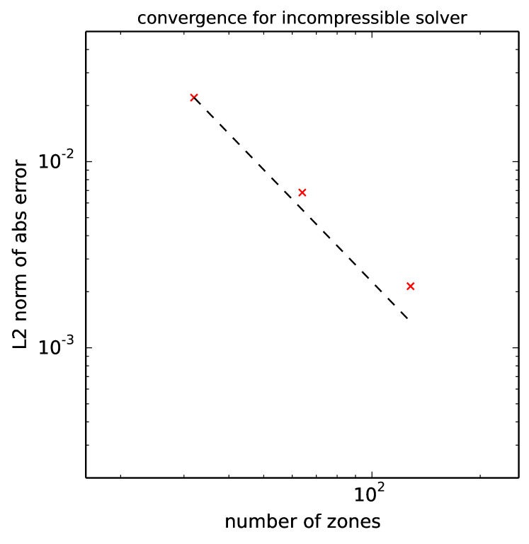
Figure 10: Convergence of the incompressible solver. These tests were run with ./pyro.py incompressible converge inputs.converge.32, and then with the inputs.converge.64 and inputs.converge.128 inputs files. The error with respect to the analytic solution was computed using the analysis/incomp_converge_error.py script.

A standard convergence test for incompressible flow was described by Minion (1996). There, the initial velocity field is:

$$u(x,y) =1-2\cos(2\pi x)\sin(2\pi y)$$ (33)

$$v(x,y) =1+2\sin(2\pi x)\cos(2\pi y)$$ (34)

and the solution at a later time is

$$u(x,y,t) =1-2\cos(2\pi(x-t))\sin(2\pi(y-t))$$ (35)

$$v(x,y,t) =1+2\sin(2\pi(x-t))\cos(2\pi(y-t))$$ (36)

By comparing the numerical solution to the analytic solution, we can compute the error. We use a fixed $\Delta t/\Delta x$ and run at several resolutions. Figure 10 shows the results. We see nearly second-order convergence—the departure is due to the use of the limiters.

3.5.2 Explorations for students

• Add viscosity to the system. This will require doing 2 parabolic solves (one for each velocity component). These solves will look like the diffusion operation, and will update the provisional velocity field.

• Switch to a variable density system (Bell and Marcus, 1992). This will require adding a mass continuity equation that is advected and switching the projections to a variable-coefficient form (since $\rho$ now enters).

4 Summary

pyro provides the building blocks that together make up a modern astrophysical simulation code. By providing simple solvers in a python environment, students are encouraged to experiment. We showed that the core solvers perform as expected and motivated some simple (and some not-so-simple) extensions for each of the solvers.

The core algorithms in pyro are mature and provide a good basis for new students to learn the ins-and-outs of computational hydrodynamics through self-study. The code will continue to be maintained and keep up with new developments in python and software engineering, but we do not expect to add new intricacies to the existing solvers. The software engineering aspects built into pyro can provide a basis for learning about version control, regression testing, and verification and validation—at the very least by showing them these ideas exist and a giving them the ability to explore.

The code is freely available, and this paper together with the code, and the detailed derivations on the pyro website provide the guidance for students. The code and online notes are written for students to learn on their own, or as part of a class. Furthermore, a mailing list is provided to support users of the code.

Major changes in the future will focus on new systems of PDEs. We envision solvers for MHD, radiation hydrodynamcs in the flux-limited diffusion approximation, and some examples of multiphysics (like diffusion + reaction systems and the viscous Burger’s equation). These can be integrated into the same framework present now and will help introduce new ideas to the students. We will also focus on making pyro more of a laboratory to introduce students to software development practices and add unit testing to the various modules. Finally, we hope to develop some simple 1-d examples for each solver that can be run in IPython notebooks to help futher link pyro and the online notes.

References

- Agertz et al. (2007) Agertz, O., Moore, B., Stadel, J., Potter, D., Miniati, F., Read, J., Mayer, L., Gawryszczak, A., Kravtsov, A., Nordlund, Å., Pearce, F., Quilis, V., Rudd, D., Springel, V., Stone, J., Tasker, E., Teyssier, R., Wadsley, J., Walder, R., Sep. 2007. Fundamental differences between SPH and grid methods. Monthly Notices of the Royal Astronomical Society 380, 963–978.
- Almgren et al. (2010) Almgren, A. S., Beckner, V. E., Bell, J. B., Day, M. S., Howell, L. H., Joggerst, C. C., Lijewski, M. J., Nonaka, A., Singer, M., Zingale, M., Jun. 2010. CASTRO: A New Compressible Astrophysical Solver. I. Hydrodynamics and Self-gravity. Astrophys J 715, 1221–1238.
- Almgren et al. (1996) Almgren, A. S., Bell, J. B., Szymczak, W. G., Mar. 1996. A numerical method for the incompressible Navier-Stokes equations based on an approximate projection. SIAM J. Sci. Comput. 17 (2), 358–369.
- Bell et al. (1989) Bell, J. B., Colella, P., Glaz, H. M., Dec. 1989. A Second Order Projection Method for the Incompressible Navier-Stokes Equations. Journal of Computational Physics 85, 257.
- Bell et al. (1991) Bell, J. B., Colella, P., Howell, L. H., Jun. 1991. An efficient second-order projection method for viscous incompressible flow. In: Proceedings of the Tenth AIAA Computational Fluid Dynamics Conference. AIAA, pp. 360–367, see also: https://seesar.lbl.gov/anag/publications/colella/A_2_10.pdf.
- Bell et al. (1988) Bell, J. B., Dawson, C. N., Shubin, G. R., 1988. An unsplit, higher order Godunov method for scalar conservation laws in multiple dimensions. Journal of Computational Physics 74, 1–24.
- Bell et al. (2004) Bell, J. B., Day, M. S., Rendleman, C. A., Woosley, S. E., Zingale, M. A., 2004. Adaptive low Mach number simulations of nuclear flame microphysics. Journal of Computational Physics 195 (2), 677–694.
- Bell and Marcus (1992) Bell, J. B., Marcus, D. L., 1992. A second-order projection method for variable-density flows. Journal of Computational Physics 101 (2), 334 – 348.
- Briggs et al. (2000) Briggs, W. L., Henson, V.-E., McCormick, S. F., 2000. A Multigrid Tutorial, 2nd Ed. SIAM.
- Chorin (1968) Chorin, A. J., 1968. Numerical solution of the Navier-Stokes equations. Math. Comp. 22, 745–762.
- Colella (1985) Colella, P., 1985. A direct Eulerian MUSCL scheme for gas dynamics. SIAM J Sci Stat Comput 6 (1), 104–117.
- Colella (1990) Colella, P., Mar. 1990. Multidimensional upwind methods for hyperbolic conservation laws. Journal of Computational Physics 87, 171–200.
- Colella and Woodward (1984) Colella, P., Woodward, P. R., Sep. 1984. The Piecewise Parabolic Method (PPM) for Gas-Dynamical Simulations. Journal of Computational Physics 54, 174–201.
- Ferland (2002) Ferland, G., Oct. 2002. Reliability in the Face of Complexity; The Challenge of High-End Scientific Computing. ArXiv Astrophysics e-prints.
- Flash Center for Computational Science (2014) Flash Center for Computational Science, 2014. Flash user’s guide, version 4.2 http://flash.uchicago.edu/site/flashcode/user_support/flash4_ug_4p2/.
- Fryxell et al. (2000) Fryxell, B., Olson, K., Ricker, P., Timmes, F. X., Zingale, M., Lamb, D. Q., MacNeice, P., Rosner, R., Truran, J. W., Tufo, H., Nov. 2000. FLASH: An adaptive mesh hydrodynamics code for modeling astrophysical thermonuclear flashes. Astrophysical Journal Supplement 131, 273–334.
- Hubber et al. (2013) Hubber, D. A., Falle, S. A. E. G., Goodwin, S. P., Jun. 2013. Convergence of AMR and SPH simulations - I. Hydrodynamical resolution and convergence tests. Monthly Notices of the Royal Astronomical Society 432, 711–727.
- Kamm and Timmes (2007) Kamm, J. R., Timmes, F. X., 2007Submitted to ApJ supplement, May 2007, see http://cococubed.asu.edu/code_pages/sedov.shtml.
- LeVeque (2002) LeVeque, R. J., 2002. Finite-Volume Methods for Hyperbolic Problems. Cambridge University Press.
- Martin and Colella (2000) Martin, D. F., Colella, P., Sep. 2000. A Cell-Centered Adaptive Projection Method for the Incompressible Euler Equations. Journal of Computational Physics 163, 271–312.
- Miller and Colella (2002) Miller, G. H., Colella, P., Nov. 2002. A Conservative Three-Dimensional Eulerian Method for Coupled Solid-Fluid Shock Capturing. Journal of Computational Physics 183, 26–82.
- Minion (1996) Minion, M. L., 1996. A Projection Method for Locally Refined Grids. Journal of Computational Physics 127, 158–177.
- Nonaka et al. (2010) Nonaka, A., Almgren, A. S., Bell, J. B., Lijewski, M. J., Malone, C. M., Zingale, M. ., 2010. MAESTRO:an adaptive low mach number hydrodynamics algorithm for stellar flows. Astrophysical Journal Supplement 188, 358–383.
- Schulz-Rinne et al. (1993) Schulz-Rinne, C. W., Collins, J. P., Glaz, H. M., 1993. Numerical Solution of the Riemann Problem for Two-Dimensional Gas Dynamics. SIAM J Sci Comput 14 (6), 1394–1414.
- Sedov (1959) Sedov, L. I., 1959. Similarity and Dimensional Methods in Mechanics. Academic Press, translated from the 4th Russian Ed.
- Shamir et al. (2013) Shamir, L., Wallin, J. F., Allen, A., Berriman, B., Teuben, P., Nemiroff, R. J., Mink, J., Hanisch, R. J., DuPrie, K., Feb. 2013. Practices in source code sharing in astrophysics. Astronomy and Computing 1, 54–58.
- Sod (1978) Sod, G. A., Apr. 1978. A survey of several finite difference methods for systems of nonlinear hyperbolic conservation laws. Journal of Computational Physics 27, 1–31.
- Stone et al. (2008) Stone, J. M., Gardiner, T. A., Teuben, P., Hawley, J. F., Simon, J. B., Sep. 2008. Athena: A New Code for Astrophysical MHD. Astrophys J Suppl S 178, 137–177.
- Strang (1968) Strang, G., 1968. On the construction and comparison of difference schemes. SIAM J. Numerical Analysis 5, 506–517.
- Swesty and Myra (2009) Swesty, F. D., Myra, E. S., Mar. 2009. A Numerical Algorithm for Modeling Multigroup Neutrino-Radiation Hydrodynamics in Two Spatial Dimensions. Astrophysical Journal Supplement 181, 1–52.
- Toro (1997) Toro, E. F., 1997. Riemann Solvers and Numerical Methods for Fluid Dynamics. Springer.
- Turk (2013) Turk, M. J., Jan. 2013. How to Scale a Code in the Human Dimension. ArXiv e-prints.
- Turk et al. (2011) Turk, M. J., Smith, B. D., Oishi, J. S., Skory, S., Skillman, S. W., Abel, T., Norman, M. L., Jan. 2011. yt: A Multi-code Analysis Toolkit for Astrophysical Simulation Data. Astrophysical Journal Supplement 192, 9.
- Wilson et al. (2012) Wilson, G., Aruliah, D. A., Titus Brown, C., Chue Hong, N. P., Davis, M., Guy, R. T., Haddock, S. H. D., Huff, K., Mitchell, I. M., Plumbley, M., Waugh, B., White, E. P., Wilson, P., Sep. 2012. Best Practices for Scientific Computing. ArXiv e-prints.
- Zingale et al. (2002) Zingale, M., Dursi, L. J., ZuHone, J., Calder, A. C., Fryxell, B., Plewa, T., Truran, J. W., Caceres, A., Olson, K., Ricker, P. M., Riley, K., Rosner, R., Siegel, A., Timmes, F. X., Vladimirova, N., Dec. 2002. Mapping Initial Hydrostatic Models in Godunov Codes. Astrophys J Suppl S 143, 539–565.