Pseudopotentials for correlated electron systems

Abstract

A scheme is developed for creating pseudopotentials for use in correlated-electron calculations. Pseudopotentials for the light elements H, Li, Be, B, C, N, O, and F, are reported, based on data from high-level quantum chemical calculations. Results obtained with these correlated electron pseudopotentials (CEPPs) are compared with data for atomic energy levels and the dissociation energies, molecular geometries and zero-point vibrational energies of small molecules obtained from coupled cluster single double triple (CCSD(T)) calculations with large basis sets. The CEPPs give better results in correlated-electron calculations than Hartree-Fock-based pseudopotentials available in the literature.

I Introduction

Pseudopotentials (also known as effective core potentials) are used to replace the chemically inert core electrons within electronic structure calculations. The use of pseudopotentials reduces the number of electrons that must be treated explicitly, and reduces the size of the basis set required to represent the one-electron orbitals. Pseudopotentials are particularly useful for heavy elements because eliminating the numerous core electrons greatly increases the efficiency of the calculations. Pseudopotentials are also used for light elements, even for hydrogen, because it can be advantageous to work with smooth pseudo-orbitals.

The atomic pseudopotentials that we describe here can be used with a range of many-body techniques, including quantum chemical methods. However, our interest is mainly in quantum Monte Carlo (QMC) calculations using the variational quantum Monte Carlo (VMC) and the more accurate diffusion quantum Monte Carlo (DMC) methods. Ceperley-Alder_1980 , Foulkes_QMC_review , Casino_reference , Lester_review_2012 These approaches can provide accurate energies with a computational cost that scales with the number of particles, $N$, as approximately $N^{3}-N^{4}$, which is better than other correlated wave function methods. The scaling of the computational cost of QMC calculations with atomic number $Z$ is, however, approximately $Z^{5}-Z^{6.5}$.Ceperley_1986 , Ma_2005_all_electron_atoms Using a pseudopotential reduces the effective value of $Z$ and makes QMC calculations feasible for heavy atoms. The relatively small memory requirements of QMC calculations also facilitates applications on massively parallel computers.

In many quantum chemical methods it is possible to use a frozen-core approximation to reduce the computational effort, but it has not so far proved possible to implement a frozen-core approximation in a straightforward manner within the VMC and DMC methods, and therefore pseudopotentials have been used instead. In addition, core-polarization effects can be included within the pseudopotential formalism,muller_1984 , shirley_1993 , lee_2000 so that the calculations go beyond the frozen-core approximation. The plane wave basis sets often used in Hartree-Fock (HF) and density functional theory (DFT) calculations for extended systems have the advantage that they can be improved systematically by increasing a single parameter, the plane wave cutoff energy. Correlated electron calculations have recently been performed using plane wave basis sets,Booth_2012_FCIQMC for which pseudopotentials are almost always used to ensure that the required basis set is of a reasonable size.

Calculations using smooth HF-based pseudopotentials Trail_2005_asymptotic , Trail_2005_pseudopotentials , Burkatzki_2007 , Burkatzki_2008 , BFD_website have yielded good results in correlated electron calculations, which appear to be superior to those obtained with DFT-based pseudopotentials.Greeff_1998 The HF-based pseudopotentials do not include correlation effects, and it is likely that more accurate pseudopotentials could be developed for correlated-electron calculations by starting from a correlated-electron theory. Acioli and Ceperleyacioli_1994 showed that pseudopotentials can be formulated within many-body theory using the density matrix.

In this paper we describe a scheme based on the density matrix for generating atomic pseudopotentials using data from correlated electron calculations. Correlated electron pseudopotentials (CEPPs) are generated for the H, Li, Be, B, C, N, O and F atoms. We choose first row atoms as they allow the use of the same basis set for AE and pseudopotential calculations, resulting in a consistent basis set error. For second row atoms and beyond such a choice is in principle possible, but in practice is numerically problematic. Neither He or Ne are considered due to the absence of experimental molecular data. To generate the CEPPs we use a combination of data from multi-configuration Hartree-Fock (MCHF)fischer_1997 atomic calculations performed on a radial grid using the ATSP2K codeatsp2k , and ab initio data for atomic core polarizabilities. The CEPPs are tested by comparing with results obtained from all-electron (AE) coupled-cluster single double triple CCSD(T) calculations performed with large Gaussian basis sets and the MOLPROmolpro code. We perform tests for atomic energy levels, ionization energies and electron affinities, and for the relaxed geometries, well depths, and total zero-point vibrational energies (ZPVEs) of 35 small molecules. We also compare our CCSD(T) results with a set of highly accurate experimental, semi-empirical, and ab initio data, which are referred to in the text as ‘accurate’. The semi-empirical results are used only when they have been considered to be more accurate than the available experimental data.

We have constructed our CEPPs using atomic states with a single valence electron, which are therefore ionized states for all atoms considered, except H and Li. There is no need to use highly ionized states to generate pseudopotentials within single particle theories, such as HF and DFT, because the construction of the pseudo-atom and resulting pseudopotential is straightforward. In the many-body case, however, the construction of the pseudo-density matrix and associated pseudo-Hamiltonian describing an atom with more than one valence electron is a challenging task, as discussed in Sec. II.1. The error due to transferring a pseudopotential from the highly ionized environment in which it is constructed to neutral or near neutral environments is partially corrected by modifying the ionic calculations. The remaining error is part of that tested by our CCSD(T) calculations.

The paper is arranged in three parts. In Sec. II we describe our method for generating the CEPPs, which is divided into subsections on: II.1 theory of many-body pseudo-atoms; II.2 theory of pseudopotentials for single-valence-electron atoms; II.3 a discussion of more subtle aspects of the generation and implementation; and II.4 parameterization in a standard form for quantum chemistry packages. The results obtained with various pseudopotentials are presented in Sec. III, which is divided into subsections on: III.1 energy levels for isolated atoms with a single-valence electron; III.2 ionization energies and electron affinities for isolated atoms; III.3 optimum geometries for small molecules; III.4 atomization energies for small molecules; and III.5 ZPVEs for small molecules. Results for optimum geometries, atomization energies (with ZPVEs removed), and ZPVEs for small molecules, are compared with AE CCSD(T) data, ‘accurate’ values, and results obtained using uncorrelated pseudopotentials available in the literature. The paper is concluded by a short summary.

Atomic units are used, unless otherwise indicated.

II Method for generating the CEPPs

II.1 Theory of many-body pseudo-atoms

The many-body density matrix for a $p$-electron atom is

$$\Gamma^{p}(\mathbf{r}_{1}\ldots\mathbf{r}_{p};\mathbf{r}_{1}^{\prime}\ldots\mathbf{r}_{p}^{\prime})=\Psi^{*}(\mathbf{r}_{1}\ldots\mathbf{r}_{p})\,\Psi(\mathbf{r}_{1}^{\prime}\ldots\mathbf{r}_{p}^{\prime}),$$ (1)

where $\Psi$ is a many-body wave function. In order to reproduce the scattering properties of the $p$-electron system using a pseudopotential describing $n$ ($\leq p$) “valence” electrons, we define a spherical core region centered on the nucleus (that is, for any $|\mathbf{r}_{i}|\leq r_{c}$). We then reduce the full density matrix to an $n$-electron density matrix outside of the core region where all $|\mathbf{r}_{i}|>r_{c}$, and continue the $n$-electron density matrix with some model form for any $|\mathbf{r}_{i}|\leq r_{c}$. Details of this generalization of the one-body Lüders relationLuders_1955 to many-body systems are given by Acioli and Ceperleyacioli_1994 .

The reduction of the $p$-body density matrix to a $n$-body form is accomplished by integrating over $p-n$ electron coordinates:

$$\Gamma^{n}(\mathbf{r}_{1}\ldots\mathbf{r}_{n};\mathbf{r}_{1}^{\prime}\ldots\mathbf{r}_{n}^{\prime})={p\choose n}\int d\mathbf{r}_{n+1}\ldots\mathbf{r}_{p}\Gamma^{p}(\mathbf{r}_{1}\ldots\mathbf{r}_{n},\mathbf{r}_{n+1}\ldots\mathbf{r}_{p};\mathbf{r}_{1}^{\prime}\ldots\mathbf{r}_{n}^{\prime},\mathbf{r}_{n+1}\ldots\mathbf{r}_{p}).$$ (2)

$\Gamma^{n}$ is the $n$-body density matrix for $n$ electrons for all $|\mathbf{r}_{i}|>r_{c}$, which is the quantity that must be preserved so that the $n$-body pseudopotential reproduces the scattering properties (to first order in the energy) of the $p$-body system. To reproduce the scattering of the all-electron system we define the pseudo-density matrix outside of the core region by

$$\tilde{\Gamma}^{n}(\mathbf{r}_{1}\ldots\mathbf{r}_{n};\mathbf{r}_{1}^{\prime}\ldots\mathbf{r}_{n}^{\prime})=\Gamma^{n}(\mathbf{r}_{1} \ldots \mathbf{r}_{n};\mathbf{r}_{1}^{\prime}\ldots\mathbf{r}_{n}^{\prime})$$ (3)

$$\forall\ |\mathbf{r}_{i}|,|\mathbf{r}_{i}^{\prime}|>r_{c},$$

with $\tilde{\Gamma}^{n}$ for any $|\mathbf{r}_{i}|,|\mathbf{r}_{i}^{\prime}|<r_{c}$ defined such that it is correctly normalized and well behaved.

Standard norm-conserving independent electron pseudopotentials Hamann_pseudopotentials_1979 are defined using valence orbitals only, but the reduced density matrix considered so far contains a contribution from the core orbitals. Consequently, for independent electrons, a pseudopotential defined from the reduced density matrix cannot be equivalent to the standard norm-conserving pseudopotential. To allow the two to be equivalent we define a modified density matrix. We separate the underlying wave function into core and valence parts, confine the core part to the core region, construct a $p$-body density matrix, and reduce it to a modified $n$-body matrix. This is achieved by expressing $\Psi$ as a sum of determinants

$$\Psi(\mathbf{r}_{1}\ldots\mathbf{r}_{p})=\sum_{all}w_{i}D_{i}(\mathbf{r}_{1}\ldots\mathbf{r}_{p}),$$ (4)

where the $w_{i}$ are coefficients. The determinants are formed from the Natural Orbitals (NOs), $\psi_{k}$, which are eigenfunctions of the density matrix with occupation numbers, $o_{k}$. The $n_{c}=(p-n)/2$ NOs with the largest occupation numbers, $o_{k}$, are identified as the core NOs. The determinants containing one or more core NOs are classified as core determinants, $D^{c}_{i}$, while the others are classified as valence determinants, $D^{v}_{i}$. In this notation $\Psi$ is expressed as

$$\Psi(\mathbf{r}_{1}\ldots\mathbf{r}_{p}) = \Psi_{v}(\mathbf{r}_{1}\ldots\mathbf{r}_{p})+\Psi_{c}(\mathbf{r}_{1}\ldots\mathbf{r}_{p})$$

$$= \sum_{j}w_{j}D^{v}_{j}(\mathbf{r}_{1}\ldots\mathbf{r}_{p})+\sum_{j}w_{j}D^{c}_{j}(\mathbf{r}_{1}\ldots\mathbf{r}_{p})$$

where $\Psi_{v}$ and $\Psi_{c}$ are taken to be the valence and core components of the wave function. Note that for the special case of a HF wave function the sole determinant would be classified as a core determinant.

In the next step the core NOs present in each $D^{c}_{i}$ are modified such that they are zero outside of the core region, which gives a modified wave function,

$$\Psi_{m}(\mathbf{r}_{1}\ldots\mathbf{r}_{p})=\left\{\begin{array}[]{ll}\Psi_{v}(\mathbf{r}_{1}\ldots\mathbf{r}_{p})&\forall\ |\mathbf{r}_{i}|>r_{c}\\ \Psi_{v}(\mathbf{r}_{1}\ldots\mathbf{r}_{p})+\Psi_{c}(\mathbf{r}_{1}\ldots\mathbf{r}_{p})&\textrm{otherwise},\end{array}\right.$$

and a modified density matrix

$$\Gamma^{p}_{m}(\mathbf{r}_{1}\ldots\mathbf{r}_{p};\mathbf{r}_{1}^{\prime}\ldots\mathbf{r}_{p}^{\prime})=\Psi^{*}_{m}(\mathbf{r}_{1}\ldots\mathbf{r}_{p})\Psi_{m}(\mathbf{r}_{1}^{\prime}\ldots\mathbf{r}_{p}^{\prime}).$$ (6)

This modification is desirable for the same reason as in the independent particle case; the scattering properties of the pseudo-system are modified by a very small amount, but significantly smaller values of $r_{c}$ can be used. It is important to note that explicit modification of the core NOs is neither required nor used in the CEPP generation procedure described below, and the remaining non-core NOs are not modified. This aspect of our scheme is essentially a many-body generalization of the removal of core orbitals in the generation of standard DFT or HF norm-conserving pseudopotentials.

Reduction to a $n$-body matrix with all coordinates constrained to lie outside of the core region provides

$$\tilde{\Gamma}^{n}_{m}(\mathbf{r}_{1}\ldots\mathbf{r}_{n};\mathbf{r}_{1}^{\prime}\ldots\mathbf{r}_{n}^{\prime}) = {p\choose n}\int d\mathbf{r}_{n+1}\ldots\mathbf{r}_{p}\Gamma^{p}_{m}(\mathbf{r}_{1}\ldots\mathbf{r}_{n},\mathbf{r}_{n+1}\ldots\mathbf{r}_{p};\mathbf{r}_{1}^{\prime}\ldots\mathbf{r}_{n}^{\prime},\mathbf{r}_{n+1}\ldots\mathbf{r}_{p})$$ (7)

$$= {p\choose n}\int d\mathbf{r}_{n+1}\ldots\mathbf{r}_{p}\Psi_{v}^{*}(\mathbf{r}_{1}\ldots\mathbf{r}_{n},\mathbf{r}_{n+1}\ldots\mathbf{r}_{p})\Psi_{v}(\mathbf{r}_{1}^{\prime}\ldots\mathbf{r}_{n}^{\prime},\mathbf{r}_{n+1}\ldots\mathbf{r}_{p})\ \forall\ |\mathbf{r}_{i}|,|\mathbf{r}_{i}^{\prime}|>r_{c}.$$

An important property of this modification and reduction procedure is that although core determinants do not contribute to $\Gamma^{p}_{m}$ outside of the core region, they do contribute to $\tilde{\Gamma}^{n}_{m}$ outside of the core region. It is this property that ensures that the CEPP is equivalent to a standard norm-conserving HF pseudopotential when the multi-determinant expansion is replaced by a single (core) determinant. A proof of this property is given in the appendix.

The density matrix $\tilde{\Gamma}^{n}$ must be preserved for a $n$-body system to reproduce the scattering properties of the $p$-body all-electron atom, but $\tilde{\Gamma}^{n}_{m}$ must be preserved for a $n$-body system to reproduce the scattering properties of the $p$-body all-electron atom with the core electrons constrained to lie within the core region.

Note that the division of $\Psi$ into core and valence parts is not unique. Our choice can, however, be justified by noting that the NOs provide the most efficient orbital representation of a wave function as a sum of determinants, and that the NO occupation numbers associated with occupied (unoccupied) orbitals are the largest (smallest) possible for all choices of orbitals.davidson_1972

In principle the next step should be to define the $n$-body density matrix in the core region $|\mathbf{r}_{i}|,|\mathbf{r}_{i}^{\prime}|<r_{c}$ in such a manner that there are $n$ pseudo-electrons and the density-matrix is smooth. This is a highly non-trivial problem. Even if this could be solved, we would then need to invert the many-body quantum Schrödinger equation to obtain a potential whose ground state has density matrix $\tilde{\Gamma}^{n}_{m}$. Again, this is a highly non-trivial problem to which a solution would in general be a $n$-body effective potential. To put this another way, in addition to the familiar core-electron pseudo-interaction naturally identifiable as a pseudopotential, there would also be core-electron-electron pseudo-interactions, etc., up to and including a $n+1$-body interaction.

To avoid this difficulty we consider only the special case of a single valence electron. The $n$-body modified density matrix is then given by

$$\Gamma_{m}^{1}(\mathbf{r};\mathbf{r}^{\prime})=\sum_{i>n_{c}}o_{i}\psi^{*}_{i}(\mathbf{r})\psi_{i}(\mathbf{r}^{\prime})\ \ \textrm{for}\ |\mathbf{r}|,|\mathbf{r}^{\prime}|>r_{c},$$ (8)

where the $\psi_{i}$ are the non-core unmodified NOs with indices ordered by decreasing $o_{i}$. Note that although a valid density matrix must be representable by a complete set of orthonormal functions, this condition does not invalidate Eq. (8). Orthonormality is allowed since our definition is over a subspace only, and completeness is allowed since we may introduce a subset of additional NOs with zero occupancy that do not contribute to the sum.

Since there is only one valence electron, the charge density contains the same information as the density matrix and we can work in terms of the pseudo-density, $\tilde{\rho}$, defined as

$$\tilde{\rho}(\mathbf{r})=\left\{\begin{array}[]{ll}\Gamma_{m}^{1}(\mathbf{r};\mathbf{r})&|\mathbf{r}|>r_{c}\\ \phi^{2}(\mathbf{r})&|\mathbf{r}|\leq r_{c},\end{array}\right.$$

with $\phi^{2}$ constructed to give the required particle number and satisfy various smoothness conditions. Finding the one-body potential for which $\tilde{\rho}$ is the ground state is then straightforward.

Before describing the implementation of such an inversion procedure, it is worth clarifying the separation of core and valence electrons used above. This separation procedure is a natural generalization of mean-field norm-conserving pseudopotential theory to many-body theory, is equivalent for non-interacting electrons in a mean-field, and is no more ad hoc than the well established procedure of removing core orbitals in mean-field pseudopotential theory. The pseudopotential provided by the inversion procedure describes the effect of core electrons on valence electrons, including correlation. From this perspective it is apparent that the CEPP fits naturally into the methodology of correlated wave function methods. The effects of correlation involving core electrons is described by the external potential part of the (pseudo-)Hamiltonian, whereas correlation between valence electrons remains a direct consequence of electron-electron interactions. For example, a ‘HF’ calculation using CEPPs includes all correlation except that between valence electrons, and post-HF methods naturally add the correlation between valence electrons to provide a complete description of the correlation effects.

II.2 Pseudopotentials for single-valence-electron systems

To create a pseudopotential for a single-valence-electron system we calculate a one-body potential that generates the density (and therefore the one-body density matrix) of the all-electron correlated atom outside of the core region. We calculate the NOs and occupation numbers on a numerical grid using the ATSP2K codeatsp2k . Core electron excitations are included in the active space (AS) so as to describe core-valence and intra-core correlation. The finite AS manifests itself as the requirement that only a finite number of orbitals can be included in the calculation, with each indexed by an angular momentum eigenvalue $l$ and an index analogous to the primary quantum number of hydrogenic atoms, $n$. We have employed the largest ranges of $n$ and $l$ that avoid numerical errors arising from linear dependence problems which, in practice, corresponds to $n\leq 6$ and $l\leq 3$, with the removal of one or two $n=6$, high $l$ orbitals for Li, Be, and B. These ranges, together with the single and double excitations of the core and valence electrons, define the AS used.

The lowest energy states of different symmetries are considered in order to construct potentials for the $s$, $p$ and $d$ angular momentum channels of a non-local pseudopotential. For example, the MCHF data for carbon are generated for the C³⁺ ion in the $1s^{2}2s\ (2S)$, $1s^{2}2p\ (2P)$ and $1s^{2}3d\ (2D)$ configurations.

We divide the radial space into three regions, in a manner similar to Lee et al.lee_2000 , defining the pseudopotential and pseudo-orbital separately in each region. The potential for each angular momentum channel $l$ is written as

$$V_{l}(r)=\left\{\begin{array}[]{rl}V_{I}(r)&0\leq r<r_{c}\\ V_{II}(r)&r_{c}\leq r<r_{0}\\ V_{III}(r)&r_{0}\leq r.\end{array}\right.$$ (9)

The core region is denoted by $I$, and the outer part is divided into two regions, $II$ and $III$. In principle the latter division is not necessary, but it is useful in controlling the numerical problems that arise far from the nucleus where the density decreases exponentially.

In region $III$ we take the potential to have the form

$$V_{III}=-\frac{Z_{v}}{r}-\frac{1}{2}\frac{\alpha}{r^{4}},$$ (10)

which is the sum of terms due to the valence charge $Z_{v}=Z-2n_{c}$, and core-valence correlation effects, with the latter described by a core polarization potential (CPP). The parameter $\alpha$ is the dipole core-polarization parameter. Higher order terms (corresponding to quadrupole polarizability and higher) are not considered here since they are negligible, provided $r_{0}$ is sufficiently large. This form provides the correct asymptotic potential far from the nucleus.

The pseudopotential in region $II$ is constructed directly from the MCHF charge density. A pseudo-orbital is defined by $u=\left[\tilde{\rho}_{l}\right]^{1/2}$ and the pseudopotential is obtained by inverting the radial Schrödinger equation:

$$V_{II}=\frac{1}{2}\frac{1}{u}\frac{d^{2}u}{dr^{2}}-\frac{1}{2}\frac{l(l+1)}{r^{2}}+\epsilon.$$ (11)

It is tempting to identify $\epsilon$ with some target eigenvalue, but this is not necessary since the potential in region $I$ has not yet been defined. Instead we note that the potentials should be continuous at $r=r_{0}$, which leads to

$$\epsilon=-\frac{Z_{v}}{r_{0}}-\frac{1}{2}\frac{\alpha}{r_{0}^{4}}-\frac{1}{2}\left.\frac{1}{u}\frac{d^{2}u}{dr^{2}}\right|_{r_{0}}+\frac{1}{2}\frac{l(l+1)}{r_{0}^{2}}.$$ (12)

The potential has a very small discontinuity in its first derivative at $r=r_{0}$. The potential in region $II$+$III$ is thus defined as that which reproduces the target charge density outside of the core region. Note that $r_{0}$ must be large enough for $V_{III}$ of Eq. (10) to be accurate, but small enough for the inversion procedure to be numerically stable. We used values of $r_{0}$ ranging from 37$r_{c}$ for H to 2.3$r_{c}$ for F. The pseudo-orbital in $II$+$III$ is then generated as the solution of

$$\left[-\frac{1}{2}\frac{d^{2}}{dr^{2}}+\frac{1}{2}\frac{l(l+1)}{r^{2}}+V_{I}-\epsilon\right]\phi(r)=0,$$ (13)

which is obtained by integrating from a large $r$ of about 50-100 a.u. down to $r_{c}$. At large $r$ the orbital is taken to be a decaying Whittaker function of the second kind, which is an exact solution of the Schrödinger equation with potential $-Z_{v}/r$. $\phi$ is then normalized in region $II$+$III$ such that

$$4\pi\int_{r_{c}}^{+\infty}\phi^{2}r^{2}dr=4\pi\int_{r_{c}}^{+\infty}u^{2}r^{2}dr.$$ (14)

The pseudo-orbital in region $I$ is chosen to be of a standard formTroullier_1991

$$\phi=r^{l+1}\exp\left[\sum_{k=0}^{6}a_{2k}\,r^{2k}\right]\ \ \ \ 0\leq r<r_{c},$$ (15)

where the parameters $\{a_{2k}\}$ are defined by seven constraints: continuity of the value and first four derivatives of $\phi$ at $r_{c}$, $V^{\prime\prime}_{I}(0)=0$, and norm conservation in region $I$ associated with Eq. (14),

$$4\pi\int_{0}^{r_{c}}\phi^{2}r^{2}dr=1-4\pi\int_{r_{c}}^{+\infty}u^{2}r^{2}dr.$$ (16)

Inverting the Schrödinger equation in region $I$ provides the potential as

$$V_{I}=\frac{1}{2}\frac{1}{\phi}\frac{d^{2}\phi}{dr^{2}}-\frac{1}{2}\frac{l(l+1)}{r^{2}}+\epsilon.$$ (17)

We now have the effective potential in regions $I$, $II$, and $III$ for which the lowest one-electron eigenstate with $\epsilon$ and $\phi$ has the same norm as $u$ in region $I$.

In our scheme we provide a target density, $\tilde{\rho}$, in regions $II+III$, which results in the density $\phi^{2}$ in regions $I+II+III$. Before commencing we clarify the relationship between $\tilde{\rho}$ and $\phi^{2}$ in region $II+III$. For the ideal case where an exact $\tilde{\rho}$ is available we could take the limit $r_{0}\rightarrow\infty$, so that $\alpha$ would not be required (core polarization effects would still be present since the AE wave function is correlated). Furthermore, we would have $\epsilon=-I$, where $I$ is the exact ionization energy of the ion (for example, for carbon this would be the difference between the total energies of C³⁺ and C⁴⁺), so we would exactly reproduce the ionization energy and the charge density outside of the core region. For a limited AS (for example a HF AE calculation) the same desirable properties occur, as long as $r_{0}\rightarrow\infty$ can be used to eliminate region $III$.

Region $III$ exists when $r_{0}$ is finite, and the potential within this region is approximate. Consequently, $\epsilon\neq-I$, but it is an accurate approximation since $\epsilon$ approaches $-I$ with increasing $r_{0}$, which ensures that $\phi^{2}$ approaches $\tilde{\rho}$ with increasing $r_{0}$. To put this another way, provided that Eq. (10) is a good approximation, the pseudopotential will reproduce the AE ionization energy and (modified) density matrix outside of the core region.

Note that the quantities that must be supplied for generating the pseudopotential are the target density in region $II+III$, and the core-polarization parameter, $\alpha$. A target eigenvalue is not required.

II.3 Fixed cores and the role of the CPP

In the above discussion the pseudopotential describes the frozen core of an ion (e.g., C³⁺), whereas it would be better for the core implicit in the pseudopotential to be that of the neutral atom, as this is closer to the electronic states of interest. This difference is expected to be small, but we account for it by fixing the core orbitals to be those of a correlated neutral atom. The required orbitals and energies are obtained from two different MCHF calculations with the same AS, with all determinant expansion coefficients free to vary. First ‘relaxed core’ MCHF results are generated for the neutral atom, with all orbitals free to vary. From the resulting orbitals we select the $n_{c}$ core orbitals. Next, we perform a ‘fixed core’ MCHF calculation, including the core orbitals of the neutral atom in the AS, allowing no variation in the core orbitals, but with all the other orbitals free to vary. This provides a new set of NOs, $\{\psi_{i}\}_{fxd}$, from which we construct the target density of Eq. (II.1), and hence the ‘fixed core’ pseudopotential. This procedure is used for all of the CEPPs generated in this work, and it provides pseudopotentials that include core-valence (and intra-core) correlation effects.

Lee et al.lee_2000 have generated pseudopotentials from HF orbitals and ‘accurate’ ionization energies of ions. They evaluate corrections to both the norm and ionization energy due to fixing the core to be that of a neutral atom. These HF corrections to the target norm and eigenvalue are then used with the HF orbitals of the ion to generate pseudopotentials. The approach of Lee et al.lee_2000 may be generalized from HF to MCHF, resulting in a scheme similar to that given in this paper. At first this approach seems appealing as it includes a semi-empirical description of physical effects not present in the MCHF Hamiltonian via the target ionization energies, such as relativistic and finite nuclear mass effects. However, we have not considered this option further since the performance of such pseudopotentials was similar or marginally worse than our more ab initio pseudopotentials for all systems considered.

Some further steps are required to define the CEPP. The angular-momentum-dependent pseudopotential, $V_{l}$, (Eq. (9)) provides an ab initio representation of the interaction between a single valence electron and the core. Although this could be applied as it stands to systems containing many electrons and atoms, consideration of the semi-empirical theory of CPPs strongly suggests that we can improve on this.

So far we have used the term ‘core-valence correlation’ to refer to all atomic correlation not represented by a HF pseudopotential. Consideration of semi-empirical CPPs allows us to separate this correlation into different parts, and to include the correlation (mostly due to exchange) arising from interactions between the separate cores of a many-atom system. The potential part of the Hamiltonian, including the CPP, can be written as

$$\hat{V}_{cv}=\left[\hat{V}_{v}+\hat{V}_{e}\right]+\left[\hat{V}_{e-e}+\hat{V}_{e-I}+\hat{V}_{I-I}\right],$$ (18)

where $\hat{V}_{cv}$ represents core-core, core-valence and valence-valence correlation effects, $\hat{V}_{v}$ represents valence-valence correlation effects, and the four CPP terms provide an approximate representation of core-core and core-valence correlation effects as an induced dipole interaction. Considering the CPP terms separately, $\hat{V}_{e}$ describes a one-body valence electron potential, $\hat{V}_{e-e}$ describes a two-body valence electron potential, $\hat{V}_{e-I}$ describes a three-body core-core-electron interaction, and $\hat{V}_{I-I}$ describes a two-body inter-core interaction. Generating a pseudopotential from an isolated atom can directly provide ab initio versions of $\hat{V}_{e}$ and $\hat{V}_{e-e}$, and, since $V_{l}$ is a one-body potential generated from an ion with a single valence electron, it only provides an ab initio version of

$$\hat{V}_{cv}=\left[\hat{V}_{v}+\hat{V}_{e}\right].$$ (19)

The $V_{l}$ pseudopotential version of this quantity can be expected to be superior to the semi-empirical CPP description.

In light of this we use $V_{l}$ to provide an ab initio description of the one-body valence electron potential, but rather than ignore the other parts of the correlation we describe them using part of the semi-empirical CPP interaction. This is achieved by subtracting the one-body core-electron part of the semi-empirical CPP interaction from the ab initio pseudopotential $V_{l}$, and adding it back in as part of the full CPP correction.

Müller and Meyermuller_1984 describe alkali dimers using configuration interaction calculations together with a CPP, and report the influence of each of the CPP terms on the equilibrium geometry and binding energy. They find the $\hat{V}_{e}$ and $\hat{V}_{e-I}$ terms to be the largest and of opposite sign. These results suggest that it is desirable to include a semi-empirical representation of the correlation that is not included in $V_{l}$.

We use the parameterized CPPs of Shirley and Martinshirley_1993 , and define a modified pseudopotential

$$V^{pp}_{l}=V_{l}-\hat{V}_{e}=V_{l}+\frac{1}{2}f^{2}(r/\bar{r}_{l})\frac{\alpha}{r^{4}},$$ (20)

where $f(x)=(1-e^{-x^{2}})^{2}$ is a short range truncation function used to remove the unphysical singularity at $r=0$, the $\bar{r}_{l}$ are empirically defined cutoff radii for this truncation function, and $\alpha$ is the polarizability parameter used in generating $V_{l}$. Throughout this paper the acronym CEPP refers to $V^{pp}_{l}$ used together with the CPP, and we emphasise that the one-body valence-electron potential part of the CEPP is ab initio even though the one-body valence electron potential part of the CPP is semi-empirical.

II.4 Pseudopotential parameterization

We tabulate each pseudopotential on a radial grid for use in QMC applications. However, most quantum chemistry packages require a Gaussian parameterization of the pseudopotential. Following the same procedure as Trail and Needs Trail_2005_asymptotic , Trail_2005_pseudopotentials , we use the parameterization

$$\tilde{V}^{pp}_{l}=\sum_{q=1}^{6}A_{ql}r^{n_{ql}}e^{-a_{ql}r^{2}}=\left\{\begin{array}[]{rl}Z_{v}/r+V^{pp}_{local}&l=local\\ V^{pp}_{l}-V^{pp}_{local}&l\neq local,\end{array}\right.$$ (21)

where $n_{ql}=0$, except for the local channel, for which $n_{ql}=-1$ for $q=1$, $n_{ql}=+1$ for $q=6$, and $n_{ql}=0$ otherwise. The local channel is chosen to be $l=2$.

The values of the parameters $A_{ql}$ and $a_{ql}$ are obtained by optimization. The number of parameters is reduced by imposing the constraints

$$\tilde{V}^{pp}_{l}(0)-V^{pp}_{l}(0)=\tilde{V^{\prime}}^{pp}_{l}(0)=\tilde{V^{\prime\prime}}^{pp}_{l}(0)=0,$$ (22)

which ensures that the parameterized form is approximately equal to the tabulated potential close to $r=0$. These constraints fix four and two $A_{ql}$ parameters, respectively, in the local and non-local channels.

The initial set of parameter values is obtained by taking 100 random values distributed uniformly over a suitable range, performing a least squares fit for each set, and solving for the ground state of each fitted potential. The set of parameters with the lowest error in the eigenvalue are then chosen, and used as initial values for the minimization of the penalty functionbarthelat_1977

$$\Sigma_{1}=\langle\phi_{l}|\left[\tilde{\epsilon}_{l}|\tilde{\phi}_{l}\rangle\langle\tilde{\phi}_{l}|-\epsilon_{l}|\phi_{l}\rangle\langle\phi_{l}|\right]^{2}|\phi_{l}\rangle,$$ (23)

where $(\phi_{l},\epsilon_{l})$ and $(\tilde{\phi}_{l},\tilde{\epsilon}_{l})$ are the lowest energy eigenstates for the tabulated and parameterized pseudopotential, respectively. Minimization of $\Sigma_{1}$ is terminated when $1-\langle\tilde{\phi}_{l}|\phi_{l}\rangle<10^{-6}$ and $|\tilde{\epsilon}_{l}-\epsilon_{l}|<10^{-5}$ a.u. A second penalty function,

$$\Sigma_{2}=\sum_{i=1}^{5}(\tilde{\epsilon}_{li}-\epsilon_{li})^{2},$$ (24)

was then minimized until $\max_{i}|\tilde{\epsilon}_{li}-\epsilon_{li}|<10^{-8}$ a.u. Only the lowest five states are included in $\Sigma_{2}$, since higher states are essentially hydrogenic and their energies are largely independent of the quality of the pseudopotential. The initial least-squares fitting, choice of best fit, and minimization of $\Sigma_{1}$ are employed as an effective way of selecting a good minimum among many. The second optimization stage is used to improve a useful measure of the quality of the parameterization, $\Sigma_{2}$, without significantly increasing $\Sigma_{1}$.

III Results

We generate CEPPs for H, Li, Be, B, C, N, O, and F.

For Li, Be, B, C, N, O, and F we choose there to be two core electrons and use the core-polarization parameter values of Shirley and Martinshirley_1993 . The three pseudopotential channels are generated from the densities provided by MCHF calculations for the $1s^{2}2s\ (^{2}S)$, $1s^{2}2p\ (^{2}P)$, and $1s^{2}3d\ (^{2}D)$ configurations, so that the CEPPs are generated from the neutral Li atom, and the Be¹⁺, B²⁺, C³⁺, N⁴⁺, O⁵⁺, and F⁶⁺ ions. The core radii are taken from our earlier Dirac-Fock (DF) pseudopotentialsTrail_2005_pseudopotentials .

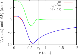
Figure 1: CEPPs (before removal of the CPP) constructed from the O⁵⁺ state. The pseudopotentials are generated from MCHF and HF densities, and the MCHF pseudopotential minus the HF pseudopotential (with identical core radii and other parameters), is shown scaled by $\times 30$.

Figure 1 shows CEPPs constructed using both the MCHF and HF charge densities of O⁵⁺ with a single $s$ electron in the lowest energy level. The differences between the two potentials are very small on the scale of the depth of the pseudopotential. The differences near $r=0$ are unimportant, but the deeper potential around $r=0.6$ a.u. of the MCHF-based CEPP is significant. The sixth ionization energy of the MCHF-based CEPP is $0.074$ eV larger than that of the HF-based CEPP, and the norm (fraction of the orbital within the pseudopotential core radius of $0.8$ a.u.) is about $0.00033$ larger for the MCHF-based CEPP. The MCHF-based CEPP is therefore slightly more attractive than the HF-based CEPP for this electronic state.

For H we choose there to be no core electrons, and hence $\alpha=0$. The three pseudopotential channels are generated from the MCHF densities (the MCHF and HF Hamiltonians are identical for the H atom) for the neutral $1s\ (^{2}S)$, $2p\ (^{2}P)$, and $3d\ (^{2}D)$ configurations. The core radii, $r_{c}$, are taken to have the same values as in our earlier workTrail_2005_pseudopotentials , with the exception of the H $d$-channel, for which we use a core radius of $r_{c}=0.8$ a.u.

In this section we assess the accuracy with which these pseudopotentials can reproduce AE and ‘accurate’ data. We begin by evaluating energy levels for single-valence-electron atoms and ions, in order to assess the quality with which the CEPPs describe a simple system without valence-valence or inter-core correlation. These calculations are performed by direct numerical integration of the radial equation. Next we move on to atoms with many valence electrons, obtaining results using the MOLPROmolpro implementation of CCSD(T) theory (and RCCSD(T) when required) with large Gaussian basis sets. We calculate atomic ionization energies and electron affinities at this level of theory, in order to assess the quality of the CEPPs for isolated atoms. Finally, we perform CCSD(T) (and RCCSD(T)) calculations on a test set of 35 small molecules, chosen by taking neutral members of the G1G1 set, removing those containing atoms other than H, Li, Be, B, C, N, O, and F, and adding H₂, BH, Be₂, B₂, C₂, and NO₂. For each molecule we evaluate: ($i$) the optimum geometry by energy minimization; ($ii$) the well depth, defined as the sum of the atomization energy and zero-point vibrational energy and denoted $D_{e}$, and ($iii$) the ZPVEs.

The CCSD(T) calculations are performed using Dunning basis setsbasis . Basis set contraction is not employed in order to allow the AS for the AE and pseudopotential calculations to be as consistent as possible, but also flexible enough to provide high accuracy. The AS for the AE calculations is defined to include core excitations. The computational cost of achieving a given level of accuracy could be reduced significantly by generating a smaller contracted even-tempered basis set for each CEPP using the Dunning model. Although the computational efficiency provided by such a choice would be desirable in future applications of the CEPPs, it does not provide the consistent error appropriate for assessing the accuracy with which the CEPP Hamiltonian reproduces AE results.

Estimates of the complete basis set limits of the total energies were obtained by extrapolating the $n=3,4$ basis set energies (for example, cc-pwCVTZ and cc-pwCVQZ) using the non-rigorous formulae

$$E_{1}(n) = a_{1}+b_{1}e^{-n}$$

$$E_{2}(n) = a_{2}+b_{2}n^{-3}$$

$$E_{est} = (a_{1}+a_{2})/2\pm(a_{1}-a_{2})/2,$$ (25)

where $E_{1}$ and $E_{2}$ underestimate and overestimate the correlation energy, respectively, and half their sum and half their difference provide estimates of the converged energy and error bounds. This is essentially a simplified version of the approach of Feller et al.Feller_2010 . Extrapolation is not used in calculating geometries or ZPVEs.

The ionization energies and electron affinities are calculated using the uncontracted aug-cc-pVnZ basis set for H, and the uncontracted aug-cc-pwCVnZ basis sets for other atoms, with $n=T,Q$. For the molecules we use uncontracted basis sets: aug-cc-pVnZ for H₂, aug-cc-pwCVnZ and aug-cc-pVnZ for LiH, aug-cc-pwCVnZ for Li₂, and cc-pwCVnZ for all others. We usually take $n=Q$ for geometry optimization and calculating ZPVEs, and $n=T,Q$ for total energies. Exceptions are described as they arise, and the well depths are evaluated using isolated neutral atom calculations performed with the same basis as for the molecule.

We compare the performance of the CEPPs within CCSD(T) with AE results, and results obtained using two other types of pseudopotential, the norm-conserving DF pseudopotentials of Trail and NeedsTrail_2005_pseudopotentials (TNDF), and the scalar-relativistic energy-consistent HF pseudopotentials of Burkatzki et al.Burkatzki_2007 (BFD). Both the BFD and TNDF pseudopotentials include relativistic effects, while the CEPPs do not. This comparison is used to investigate the changes that arise from the explicit inclusion of correlation in the pseudopotential generation process, and to test whether the CEPPs generated from single-electron ions transfer successfully to systems with multiple valence electrons and atoms. Burkatzki et al. provide contracted basis sets for use with their pseudopotentials. We do not use these basis sets, since the uncontracted Dunning basis sets we have used consistently provide better convergence properties and lower energies for first row diatomic and hydride molecules.

We take our baseline data to be that provided by AE CCSD(T) calculations, defining the error in the well depth, $D_{e}$, the geometry, and the ZPVEs as the deviation of the pseudopotential results from the AE ones. However, in each plot the ‘accurate’ data are also shown as deviations from the baseline and are discussed separately at the end of this section. We make our primary comparison of pseudopotential results with the AE baseline data in order to separate the pseudopotential errors from those present in both the AE and pseudopotential CCSD(T) calculations (for example, errors due to the finite basis sets, lack of relativistic effects, use of harmonic vibrational energies, etc). This is desirable since the magnitudes of the errors due to using the CEPPs and the CCSD(T) theory are of comparable size.

Before testing the pseudopotentials, we briefly mention the accuracy of the MCHF calculations used to generate the pseudopotentials, and the RCCSD(T) results for the same AE atoms and ions. We quantify the accuracy by expressing the difference between the calculated and HF total energies as a fraction of the difference between the ‘accurate’ and HF total energies. For the three-electron atoms and ions used to construct the pseudopotentials for Li, Be, B, C, N, O, and F, MCHF provides $\sim$98–100 % of the correlation energy, whereas RCCSD(T) provides $\sim$100 % for all of the atoms and ions. For the neutral atoms MCHF provides $\sim$98–88 % of the correlation, decreasing monotonically with increasing atomic number, and RCCSD(T) provides $\sim$100 % of the correlation energy for all of the atoms.

III.1 Energy levels for single-valence-electron atoms and ions

The accuracy of the CEPPs is first tested by calculating single-electron excitation energies using numerical integration. These energies are compared with ‘accurate’ energy levels by averaging spectral dataNIST_De over the spin-splitting using the standard formula

$$\epsilon_{nl}=\left[(l+1)\epsilon_{j=l+1/2}+l\epsilon_{j=l-1/2}\right]/\left[2l+1\right],$$ (26)

and subtracting the $n\rightarrow\infty$ limit (taken from NISTNIST_De ). Equation (26) is a natural choice as it would exactly remove spin-splitting if it arose from a perturbative treatment of spin-orbit coupling. The difference between the energy levels obtained with the tabulated CEPP and the ‘accurate’ energy levels provides a measure of the accuracy with which a pseudopotential reproduces the one-electron excitation spectrum.

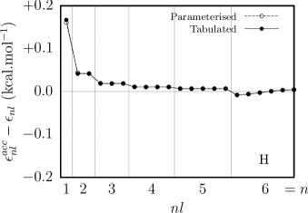
Figure 2: Difference between ‘accurate’ and CEPP excitation energies for the single-electron H atom. Both tabulated and parameterized CEPP results are shown, and the ‘accurate’ data are experimental data taken from NISTNIST_De . Results are shown in the range $n=1\ldots 6$ and $l=0\ldots 5$, with each segment containing results ordered by increasing $l$.

Figure 2 shows results for the neutral H atomNIST_H_I with the tabulated and parameterized CEPP. All of the results are well within chemical accuracy of $1$ kcal.mol^-1, and the results obtained with the parameterized and tabulated CEPPs are almost indistinguishable, with the maximum difference being $-0.006$ kcal.mol^-1 for $nl=1s$. Figure 2 does not show perfect agreement between the ‘accurate’ and CEPP excitation energies, even for the states used to construct the CEPP, with the largest difference between the ‘accurate’ and pseudo-levels being $0.17$ kcal.mol^-1 at $nl=1s$. This difference arises almost entirely from our assumption of an infinite nuclear mass and, on adjusting the energy levels using the appropriate scaling factor, the maximum value of the remaining error is $-0.013$ kcal.mol^-1 for $nl=6s$.

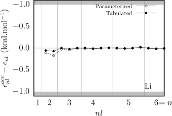
Figure 3: Difference between ‘accurate’ and CEPP excitation energies for the single-valence-electron Li atom. Both tabulated and parameterized CEPP results are shown. The ‘accurate’ data are experimentalNIST_De . Results are shown in the range $n=2\ldots 6$ and $l=0\ldots 5$ where ‘accurate’ data are available. Each segment contains results ordered by increasing $l$.

Figure 3 shows results for the neutral Li atom as the difference between the ‘accurate’ energy levels of LiNIST_Li_I and pseudo-levels obtained with the tabulated and parameterized CEPPs. The ‘accurate’ results are reproduced to well within chemical accuracy, with the largest error for the tabulated and parameterized CEPPs being $0.070$ kcal.mol^-1 (at $nl=2p$) and $0.17$ kcal.mol^-1 (at $nl=2p$), respectively. The results obtained with the parameterized and tabulated CEPPs agree to well within chemical accuracy, with a maximum difference of $-0.10$ kcal.mol^-1 at $nl=2p$.

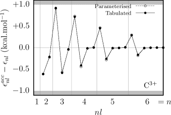
Figure 4: Same as Fig. 3, but for C³⁺.

Figure 4 shows analogous results for the C³⁺ ion. The difference between the ‘accurate’NIST_C_IV and pseudo-atom energy levels is larger than for Li, reflecting a general trend that the error increases with atomic number (for the atoms considered). The largest deviations from the ‘accurate’ data for tabulated and parameterized CEPPs are both within chemical accuracy at $-0.89$ kcal.mol^-1 (at $nl=3s$). The maximum difference between the tabulated and parameterized CEPP results of $-0.029$ kcal.mol^-1 for $nl=4p$ is smaller than the maximum difference for Li.

Figure 5: Same as Fig. 4, but for F⁶⁺.

Figure 5 shows similar results for the F⁶⁺ ion. The parameterization is accurate, with a maximum difference between the tabulated and parameterized CEPP results of $-0.074$ kcal.mol^-1 for $nl=4p$, which is smaller than that for Li. The difference between the ‘accurate’NIST_F_VII and pseudo-atom energy is larger than chemical accuracy for a number of levels, with differences of $-8.3$, $-7.7$, and $-0.7$ kcal.mol^-1 for $nl=2s,2p$ and $3d$. This is not an error due to the CEPP generation process per se, since the CEPP is designed to reproduce the properties of an ion with the core of the neutral atom. For example, consider the largest error at $nl=2s$. Generating an alternative CEPP from fully relaxed core NOs reduces this from $-7.7$ to $-4.5$ kcal.mol^-1, in good agreement with the AE MCHF value of $-4.6$ kcal.mol^-1 (and the AE CCSD(T) value of $-4.5$ kcal.mol^-1). Furthermore, this remaining error is almost entirely due to relativistic effects; including a Breit-Pauli relativistic correction in the AE MCHF calculation results in a final error of only $-0.1$ kcal.mol^-1 (AE CCSD(T) with a Douglas-Kroll-Hess Hamiltonian results in an error of $0.2$ kcal.mol^-1). This suggests that the deviation of the CEPP results from ‘accurate’ results is satisfactory, since our CEPPs have been generated to represent the cores of the neutral atoms, and to exclude relativistic effects.

We conclude that our parameterization is successful, in that the deviations of the pseudo-levels from ‘accurate’ data are sufficiently small, and the CEPPs accurately describe isolated single-valence-electron atoms. We also conclude that the deviation of the CEPP single-valence electron excitations from ‘accurate’ results is dominated by physical effects absent from the MCHF data and, for fluorine, by the fixed core correction, rather than due to deficiencies in the pseudopotential generation procedure. Note that these results provide no information on the transferability of the CEPPs between the ionic states and more neutral states.

III.2 Ionization energies and electron affinities

Here we examine the accuracy of the parameterized CEPPs with more than one electron in accounting for the ionization energies and electron affinities of isolated atoms and ions. Unlike the one-electron spectra considered above, we primarily compare with AE results, although ‘accurate’ data obtained from the NIST online databaseNIST_De are also considered.

Results were obtained at the CCSD(T) level using the aug-cc-pVnZ basis set for H, and the aug-cc-pwCVnZ basis set otherwise, with the complete basis set limit energies estimated using $n=T,Q$basis and Eqs. (III). Results were generated for AE atoms, and for the TNDF and BFD potentials and the CEPPs. Calculated ionization energies and electron affinities, together with ‘accurate’ dataNIST_De , are shown in Tables 1 and 2 for H, Li, C³⁺, and F⁶⁺. In what follows we concentrate on the differences between the CEPP and AE results.

The data for H shown in Table 1 provide ionization energies and electron affinities well within chemical accuracy of the AE values, with the CEPP results deviating from the AE data by less than $0.0035$ eV, and consistently being the most accurate of the three pseudopotentials. As for single-electron energy levels, the assumption of infinite nuclear mass results in an overestimate of the ionization energy by about $0.0073$ eV when compared with the ‘accurate’ value, see Table 1. On adjustment for finite nuclear mass, the ionization energy arising from the CEPP calculation differs from the ‘accurate’ result by only $0.004$ eV.

H
	$I_{1}$ (eV)	EA (eV)
‘Accurate’	$13.598433770784(12)$	$0.754195(19)$
AE	$13.6066(3)$	$0.7471(8)$
TNDF	$13.6104(6)$	$0.7475(8)$
BFD	$13.6102(6)$	$0.7495(8)$
CEPP	$13.6098(6)$	$0.7469(8)$
Li
	$I_{1}$ (eV)	EA (eV)
‘Accurate’	$5.391714668(22)$	$0.618049(2)$
AE	$5.3921(2)$	$0.6178(1)$
TNDF	$5.34289(2)$	$0.62685(8)$
BFD	$5.34244(2)$	$0.62719(8)$
CEPP	$5.38746(2)$	$0.62555(9)$

Table 1: Ionization energies ($I$) and electron affinities (EA) of H and Li. All-electron and pseudopotential ionization energies and electron affinities are calculated with RCCSD(T). ‘Accurate’ ionization energies are taken from NISTNIST_De , and are ab initio for H and experimental for Li. The ‘accurate’ electron affinity is from experimentaff_H , aff_Li .

As demonstrated by the data in Table 1, the Li CEPP performs very well, with the deviation from the AE results being well within chemical accuracy, with a maximum value of $0.008$ eV. The agreement with the AE results is much worse for the TNDF and BFD pseudopotentials, with the first ionization energy deviating from the AE value by about $0.043$ eV. We conclude that the Li CEPP gives more accurate results than the TNDF and BFD pseudopotentials.

The errors for C³⁺ deduced from the data in Table 2 are larger and more complex. The largest deviation from the AE results occurs for the TNDF pseudopotential ($I_{4}$), with the BFD pseudopotential providing the smallest maximum deviation ($I_{2}$). The CEPP and AE results agree to within chemical accuracy for three out of the five cases, two of which are the important lowest energy excitations of the first ionization energy and the electron affinity. Neither the BFD or TNDF results for the first ionization energy agree with the AE data to within chemical accuracy.

Table 2 also provides data for F⁶⁺, showing similar behavior to the C³⁺ case. Both the TNDF and BFD pseudopotentials reproduce the AE results to within chemical accuracy for only the electron affinity, whereas the CEPP reproduces both the first ionization energy and electron affinity to within chemical accuracy.

There are two separate sources of error in using a CEPP for isolated atoms: $(i)$ the error due to representing core-valence correlation by a static potential, and $(ii)$ the error due to generating the CEPP from an ion and using it for states that are close to neutral. To investigate the relative magnitudes of these errors we generate a second CEPP from a coreless one-electron Li²⁺ ion using the $2s\ (2S)$, $2p\ (2P)$, and $3d\ (2D)$ configurations, so that the $s$-channel reproduces the $2s$ orbital. This choice is made because it is much more important to accurately reproduce the chemically active $2s$ orbital than the $1s$ core orbital. We choose the same core radii as in earlier workTrail_2005_pseudopotentials ; $r_{c}=0.5$ a.u. for the $s$-channel and $r_{c}=0.8$ a.u. for the rest. (Results obtained with the coreless Li²⁺ CEPP are not included in Table 1.)

The second and third ionization energies obtained with the coreless Li²⁺ CEPP are not accurate as they differ from the AE and ‘accurate’ values by about $0.35$ eV. However, the first ionization energy and electron affinity are considerably more accurate than those from the Li CEPP, with an error of less than $0.0009$ eV (in comparison to $0.008$ eV from the CEPP with a core). It is clear that the coreless Li²⁺ CEPP does not represent core-valence interactions with a static potential (as there are no core electrons) and is generated from an ion, whereas the Li CEPP describes core-valence interaction with a static potential and is constructed from a neutral atom. We conclude that, at least for Li, the error due to transferring the CEPP between different ionization states is less than that due to representing core-valence correlation by a static potential. However, for both cases the error is small and is well within chemical accuracy.

The errors for carbon and fluorine include contributions from representing the core-valence interaction by a static potential and from generating the CEPP in a highly ionized state and applying it to less ionized states. Our results suggest that the sum of these errors is small since both the C⁺³ and F⁺⁶ CEPPs reproduce the AE values of the electron affinity and first ionization energy to within chemical accuracy. Finally we note that, for Li, C⁺³, and F⁺⁶, considering the deviation of the CEPP results from ‘accurate’ data does not alter our analysis significantly, and the AE results are within chemical accuracy of the ‘accurate’ data.

We conclude that CEPPs successfully reproduce ionization energies and electron affinities for isolated atoms with one or more valence electrons.

C3+
	$I_{4}$ (eV)	$I_{3}$ (eV)	$I_{2}$ (eV)	$I_{1}$ (eV)	EA (eV)
‘Accurate’	$64.49358(19)$	$47.88778(12)$	$24.3845(9)$	$11.26030$	$1.262$
AE	$64.4674(5)$	$47.874(1)$	$24.384(4)$	$11.260(2)$	$1.250(1)$
TNDF	$64.112058(5)$	$47.8901(9)$	$24.249(3)$	$11.191(2)$	$1.229(1)$
BFD	$64.45501(5)$	$48.0007(7)$	$24.225(3)$	$11.180(2)$	$1.221(1)$
CEPP	$64.46782(5)$	$48.1702(8)$	$24.479(3)$	$11.276(2)$	$1.226(1)$
F6+
	$I_{4}$ (eV)	$I_{3}$ (eV)	$I_{2}$ (eV)	$I_{1}$ (eV)	EA (eV)
‘Accurate’	$87.175(17)$	$62.7080(3)$	$34.97081(12)$	$17.42282(5)$	$3.4011895(25)$
AE	$87.209(7)$	$62.799(7)$	$34.962(10)$	$17.425(6)$	$3.431(5)$
TNDF	$87.072(4)$	$62.696(4)$	$34.873(9)$	$17.370(5)$	$3.413(5)$
BFD	$-$	$62.624(5)$	$34.863(10)$	$17.371(6)$	$3.411(5)$
CEPP	$87.528(4)$	$63.007(4)$	$35.033(9)$	$17.436(5)$	$3.412(5)$

Table 2: Ionization energies ($I$) and electron affinities (EA) of C and F. The all-electron and pseudopotential ionization energies and electron affinities are calculated using RCCSD(T). ‘Accurate’ ionization energies are taken from NISTNIST_De , and are experimental, with the exception of C($I_{2}$), F($I_{4}$), and F($I_{3}$), which are semi-empirical. The ‘accurate’ electron affinity is from experimentaff_C , aff_F .

III.3 Optimized geometries

Molecular geometries are obtained by direct minimization of the CCSD(T) energy, enforcing the known symmetry of each molecule to obtain the free parameters for optimization. We generate results for the test set of $35$ small molecules for the AE systems, and the TNDF and BFD pseudopotentials, and the CEPPs.

We have not attempted to extrapolate the geometries to the complete basis set limit, and we use the basis sets as described following Eqs. (III) with $n=Q$, except for H₂CO, H₂O₂, H₃COH, and H₄N₂, for which we use $n=T$. The molecular geometries are characterized by their bond lengths, bond angles, and dihedral angles. Deviations of these quantities from the AE CCSD(T) values are evaluated, and we seek standard chemical accuracy of $0.01$ Å. Comparison of bond lengths is straightforward, but comparison of bond angles and dihedral angles is less so. We have mapped the bond and dihedral angles to the arc of a circle of radius $1.0$ Å (a typical bond length for the molecules considered), and this arc length is compared to the standard chemical accuracy value of $0.01$ Å. To put this another way, we consider chemical accuracy for bond and dihedral angles to be $0.57^{\circ}$.

Figure 6 shows geometry parameters from optimizations with all three pseudopotentials, as deviations from the baseline AE results. (No data are available for H₂O₂ with TNDF or BFD since these calculations failed to converge.) For almost all molecules the TNDF and BFD potentials, and the CEPPs, provide molecular geometries within chemical accuracy of the AE results. The maximum deviations from the AE results for the TNDF and BFD potentials, and the CEPPs, are $0.0096$ Å (for Be₂), $0.015$ Å (for CH${}_{2}(^{3}B_{1})$), and $0.014$ Å (for H₂O₂), respectively. The mean absolute deviations (MAD) from the AE results are $0.0032$ Å, $0.0029$ Å, and $0.0041$ Å, respectively.

It is desirable to find some measure of the contribution of core-valence interaction and transferability errors to the deviation of the CEPP optimized geometries from the AE values. For LiH and Li₂ this can be achieved by briefly returning to the coreless one-electron Li²⁺ CEPP of Sec. III.2. For LiH the deviation of the optimum bond length from the AE value is reduced by $\times 1/6$ when we replace the ‘standard’ Li CEPP by the coreless Li²⁺ CEPP. Similarly, for Li₂ the coreless Li²⁺ CEPP reduces this error by $\times 1/9$. Following the same reasoning used for the ionization energies, this suggests that the error from the CEPP is mostly due to representing core-valence interaction with a static potential, and that generating a CEPP from an ion and transferring it to a neutral system introduces a relatively small error. (Results obtained using the coreless Li²⁺ CEPP are not shown in Fig. 6.)

We conclude that geometry optimization with the TNDF and BFD potentials and the CEPPs is successful in that they reproduce the AE results to within $0.015$ Å. The TNDF potentials give slightly more accurate geometries than the BFD and CEPP potentials, and the TNDF geometries are within chemical accuracy of the AE results for all of the systems studied. However, all three potentials give a good description of the geometries, with the variation in the errors between molecules being comparable to the variation in the errors between pseudopotential types.

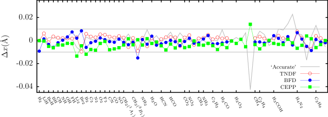
Figure 6: Deviation of spatial parameters from the baseline AE CCSD(T) results. The AE and pseudopotential results are obtained by geometry optimization as described in the text, using the TNDF and BFD pseudopotentials, and the CEPPs. The deviation of the ‘accurate’ results from AE data is shown in gray, with the ‘accurate’ data taken from NISTNIST_geom , with the exception of CH${}_{2}(^{3}B_{1})$CH2-2_geom , H₂OH2O_geom , HCOHCO_geom , and H₂O₂H2O2_geom . All ‘accurate’ spatial parameters are experimental, and the coordinates for each molecule are ordered as in the NIST database. Almost all of the pseudopotential results are within chemical accuracy (horizontal gray lines) of the AE data.

III.4 Well depths

The molecular well depth, $D_{e}$, is obtained at the optimum geometry by evaluating the difference between the CCSD(T) total energies of the molecules and their component atoms using consistent basis sets, and estimating the energies in the complete basis set limit using Eqs. (III). The basis sets used are as described following Eqs. (III).

Figure 7 shows well depths, $D_{e}$, for the TNDF and BFD potentials and the CEPPs, as deviations from the AE well depths. All of the data are calculated at the optimum geometries (no data is available for H₂O₂ with the TNDF or BFD pseudopotentials, since these calculations failed to converge). Note that Eqs. (III) provide a range of values for the error in $D_{e}$, but this range is not discernable on the scale of the plot. The smallness of this range is due to cancellation of extrapolation errors between the AE and pseudopotentials results.

Overall, the errors in the TNDF and BFD results increase with molecular size, with a maximum deviation from the AE results of $-5.7$ kcal.mol^-1 (for CO₂) and $-8.2$ kcal.mol^-1 (for H₄N₂), respectively. However, the MAD values are similar, with $2.0$ kcal.mol^-1 for the TNDF pseudopotentials and $2.2$ kcal.mol^-1 for BFD. The agreement with the AE results is, for both TNDF and BFD, well outside of chemical accuracy for most molecules, and we ascribe this, at least in part, to the absence of correlation in the generation of these pseudopotentials. Overall the TNDF pseudopotentials appear to be more accurate than BFD, but not consistently so for all of the molecules considered.

Figure 7 also shows well depths, $D_{e}$, for CEPPs as deviations from the baseline AE results. These results are consistently more accurate than for the uncorrelated pseudopotentials, with a maximum deviation from the AE results of $2.3$ kcal.mol^-1 (for N₂) and a MAD of $0.6$ kcal.mol^-1. The well depths of $27$ out of the $35$ molecules fall within chemical accuracy of the AE values.

We quantify the error in $D_{e}$ due to core-valence interaction and transferability in the same manner as for geometry optimization. Replacing the ‘standard’ Li CEPP by the coreless one-electron Li²⁺ CEPP of Sec. III.2 results in a $\times 1/30$ and $\times 1/50$ reduction in the deviation of the CEPP results from the AE results for LiH and Li₂, suggesting that the error in the CEPP arises mostly from the representation of the core-valence interaction by a potential and that the error due to transferring the CEPP from an ion to the neutral system is small. (Results obtained using the coreless Li²⁺ CEPP are not shown in Fig. 7.)

We conclude that the CEPPs provide significantly more accurate well depths than the TNDF and BFD pseudopotentials.

Figure 7: Deviation of well depths from the baseline AE CCSD(T) results. The AE and pseudopotential results are obtained at the optimum geometries as described in the text, using the TNDF and BFD pseudopotentials, and the CEPPs. ‘Accurate’ well depths are obtained by summing experimental dissociation energies and ZPVEs, with the exception of C₂Feller_2010 for which the well depth is ab initioFeller_2010 . Dissociation energies are from O’Neil and Gill oneil_De , except for BHBH_De , Be₂Be2_De , B₂B2_De , and NO₂NO2_De . Zero-point vibrational energies are from NISTNIST_geom except for Be₂Be2_De , B₂B2_De , and NONO2_De . The gray range shows the deviation of the ‘accurate’ well depths from the range of AE well depths given by Eqs. (III), and the gray horizontal lines indicate chemical accuracy.

III.5 Zero-point vibrational energies

The harmonic ZPVEs are obtained within CCSD(T) by diagonalization of the Hessian obtained from numerical energy derivatives at the optimum geometry, and summation of the contributions from each mode. We do not attempt to extrapolate this data to the complete basis set limit, and we use the basis sets as described following Eqs. (III) with $n=Q$, except for B₂, N₂, H₂CO, H₂O₂, C₂H₄, H₃COH, H₄N₂, and C₂H₆, for which we use $n=T$.

Figure 8 shows the ZPVEs obtained for the TNDF and BFD potentials and the CEPPs as deviations from the baseline AE results (no data is available for H₂O₂ with TNDF or BFD pseudopotentials, as these calculations failed to converge). For all three pseudopotentials and all molecules the ZPVEs fall well within chemical accuracy (of $1$ kcal.mol^-1) of the AE results. Of the three pseudopotential types, the CEPPs consistently provide the most accurate ZPVEs. The maximum deviations from the AE results for the TNDF and BFD potentials, and the CEPPs are $-0.15$, $-0.38$, and $0.13$ kcal.mol^-1, respectively. The MADs from the AE results are $0.05$, $0.09$, and $0.03$ kcal.mol^-1, respectively. It appears that the underestimation of the ZPVEs by the BFD pseudopotentials for some molecules is primarily due to an inadequate description of H.

We quantify the errors in the harmonic ZPVEs for the CEPPs due to core-valence interaction and transferability in the same manner as for the geometry optimization and well depth. Replacing the ‘standard’ Li CEPP by the coreless one-electron Li²⁺ CEPP of Sec. III.2 results in a $\times 1/143$ and $\times 1/6$ reduction in the differences between the CEPP and AE results for the LiH and Li₂ molecules. This suggests that the error in the CEPP ZPVE is mostly due to the representation of the core-valence interaction by a potential, with the error due to transferring the CEPP from an ion to a neutral system being relatively unimportant. (Results obtained using the coreless Li²⁺ CEPP are not shown in Fig. 8.)

We conclude that, of the three pseudopotentials, the CEPPs reproduce the AE ZPVEs to the highest accuracy. The ZPVEs calculated using the TNDF pseudopotentials are marginally less accurate. The ZPVEs calculated using the BFD pseudopotentials are significantly less accurate, with a maximum deviation from the AE results of $\times 3$ greater than for the CEPPs, but still well within chemical accuracy of the AE results.

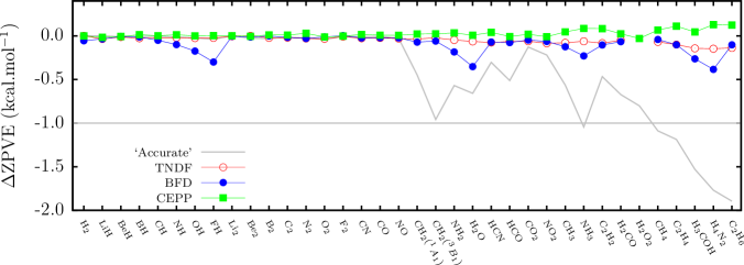
Figure 8: Deviation of the ZPVEs from the baseline AE CCSD(T) results. The AE and pseudopotential results are obtained at the optimum geometries as described in the text, using the TNDF and BFD pseudopotentials and the CEPPs. The deviation of the ‘accurate’ experimental data from the AE results is shown in gray. ‘Accurate’ ZPVEs are from NISTNIST_geom , except for Be₂Be2_De . The gray horizontal line indicates the lower bound for chemical accuracy.

III.6 All-electron CCSD(T) and ‘accurate’ data

The differences between the ‘accurate’ geometries and the AE data is significantly larger than chemical accuracy for H₂O₂, H₃COH, and H₄N₂, where the errors occur for bond or dihedral angles. Relaxing the geometry of H₂O₂ using the contracted aug-cc-pVTZ basis results in a negligible change in bond lengths, a small improvement in the bond angle, and an error in the dihedral angle which is smaller than chemical accuracy. This suggests that the error in the original calculation arose from the absence of diffuse basis functions resulting in a poor description of bond angles involving H-H interactions.

Geometry optimization for H₃COH using the contracted aug-cc-pVTZ basis set suggests a similar source of error, resulting in a negligible change in bond lengths and an error in bond angles of chemical accuracy or less. Geometry optimization of H₄N₂ using the contracted aug-cc-pVTZ appears to increase the errors in both bond angles. However, this is probably not significant given the uncertainty in the experimental values for these quantitiesH4N2_exp .

There is an underlying trend for the well depths, $D_{e}$, to be overestimated in the AE results as compared with the ‘accurate’ data. It seems reasonable to ascribe part of this error to the absence of relativistic effects since the relativistic correction provided by O’Neil and Gilloneil_De shows a similar general behavior and magnitude, decreasing the well depth by $0.0-1.1$ kcal.mol^-1. However, such a correction does not explain all of the error (particularly for B₂, CN, and NO₂).

For a detailed analysis of the remaining error due to extrapolation to the complete basis set limit and correlation missing from CCSD(T) we refer the reader to Feller and Petersonfeller_99 .

Our AE results agree with ‘accurate’ data with a similar accuracy to that achieved by Feller and Peterson, with a MAD and maximum deviation from the ‘accurate’ data of $0.95$ and $2.5$ kcal.mol^-1 for those molecules common to both their paper and ours (all of our set except for BH, Be₂, B₂, C₂, and NO₂). For comparison, taking the results of Feller and Peterson that include core-valence correlation and comparing with our ‘accurate’ data results in a MAD and maximum deviation of $0.53$ and $2.9$ kcal.mol^-1. We consider the agreement between our ab initio AE results and ‘accurate’ data to be as good as we could hope for, given the neglect of relativistic corrections, the correlation missing from CCSD(T) in the complete basis set limit (estimatedfeller_99 to be roughly $1$ kcal.mol^-1), and that the experimental errorsfeller_99 , when available, fall within the range $0.01-2.4$ kcal.mol^-1.

Overall the deviation of the ‘accurate’ well depths from the AE results is not significantly different from the deviation of the CEPP well depths from the AE data; the MADs of the AE results from the ‘accurate’ data, the CEPP results from the ‘accurate’ data, and the CEPP results from the AE results are $1.0$, $0.8$, and $0.6$ kcal.mol^-1, respectively.

The MAD of the ‘accurate’ ZPVEs from the AE results is $0.42$ kcal.mol^-1, with a maximum value of $-1.89$ kcal.mol^-1 for C₂H₆. This is significantly larger than the deviation of the CEPP results from the AE values ($0.03$ kcal.mol^-1, and a maximum of $0.13$ kcal.mol^-1 for H₄N₂).

The data shows the general trend that the calculated harmonic ZPVEs overestimate the ‘accurate’ data, with the overestimation increasing with the number of H atoms present in each molecule. This trend is particularly apparent for the 8 larger molecules on the right hand side of Fig. 8. It is also evident in the good agreement between the ‘accurate’ data and the AE results for the two largest molecules containing no hydrogen atoms, CO₂ and NO₂, and in the small error for the diatomic molecules compared with the rest of the set. Overall the deviation of the ‘accurate’ ZPVEs from the AE data appears to be dominated by cubic anharmonic effects involving hydrogen atomspfeiffer_13 , which reduce the vibrational frequencies. Such effects are not included in our AE and pseudopotential calculations, suggesting that the AE harmonic ZPVEs have provided the appropriate baseline for assessing the performance of the pseudopotentials.

IV Conclusions

We have developed a scheme for generating pseudopotentials suitable for use in correlated-electron calculations. These correlated electron pseudopotentials (CEPPs) are created using data from correlated-electron atomic MCHF calculations and ab initio core polarizabilities. We have created CEPPs for the H, Li, Be, B, C, N, O, and F atoms, although our approach can readily be applied to heavier elements. We emphasize that the full accuracy of the CEPPs is obtained only when the potential of Eq. 18 is used, made up of an ab initio one-electron term and three many-body terms taken as part of the semi-empirical CPP potential.

The CEPPs have been tested by performing CCSD(T) calculations with large Gaussian basis sets for various atoms and molecules and comparing the resulting equilibrium geometries, well depths, and zero-point vibrational energies of 35 small molecules with accurate AE results. The MAD and maximum errors in the well depths of the 35 molecules are: CEPP ($0.6$ and $2.3$ kcal.mol^-1), TNDF ($2.0$ and $-5.7$ kcal.mol^-1), and BFD ($2.2$ and $-8.2$ kcal.mol^-1). These results demonstrate the superior performance of our CEPPs for correlated systems, as compared with the uncorrelated pseudopotentials available in the literature. The results for the geometries and ZPVEs are similar for the different potentials.

Many of the CEPPs are generated in highly ionized states, but our results show that they can give highly accurate results for neutral systems. In the light of the known transferability problems that occur for norm-conserving DFT pseudopotentials this is, perhaps, a surprising feature of our results. This can be understood by noting that our CEPPs are constructed by exact inversion of the pseudo-atom Schrödinger equation, whereas a norm-conserving DFT pseudopotential is constructed by an approximate inversion of the self-consistent Kohn-Sham equations (in the sense that the exchange-correlation functional is approximate, contains self-interaction, and is linearized in the inversion process). Consequently the CEPPs can be expected to show better transferability than DFT pseudopotentials. Furthermore, it is well known that atomic cores become less responsive to valence electrons as we move to the right of each period (as in CPP theory). This suggests that although the description of core-valence interactions will become less accurate it will also exhibit a weaker dependence on the behaviour of the valence electrons. Our results are consistent with this; the transfer error for lithium was found to be negligible and as we move to the right of the period no consistent increase in error is apparent for electron affinities or first ionization energies of atoms, or for the geometries, well depths, or ZPVEs of molecules.

It would be possible to improve the CEPPs by including, for example, relativistic effects, although they are small for the light atoms considered here. Overall we conclude that the CEPPs work very well in the cases considered and that they produce better results in correlated-electron calculations than HF-based pseudopotentials available in the literature.

Tabulated and parameterized forms of the CEPPs described in this paper are given in the supplementary material.Supplemental

*

Appendix A Properties of reduced density matrices due to modified core NOs

In Sec. II.1 a many-body wave function made up of valence determinants and modified core determinants was defined and used to construct a $p$-body density matrix. This $p$-body density matrix was then reduced to a $n$-body density matrix in order to define the CEPP.

It is tempting to assume that since the core determinants of Sec. II.1 are zero outside of the core region the modified core determinants will not contribute to the $n$-body reduced density matrix (and CEPP) in this region. This is not so. To demonstrate this we consider the special case of a Hartree-Fock wave function, which is a single normalized core determinant, for which the core NOs are chosen to be zero outside of the core region.

We define the Hartree-Fock wave function as a function of all electronic co-ordinates, $\mathbf{r}_{1}\ldots\mathbf{r}_{p}$, where $|\mathbf{r}_{i=1\ldots n}|>r_{c}$, but $\mathbf{r}_{i=n+1\ldots p}$ are free to vary over all space. The Slater determinant may then be written as

$$\Psi_{\rm HF}=\frac{1}{\sqrt{p!}}\left|\begin{array}[]{cc}\mathbf{A}_{11}&\mathbf{A}_{12}\\ \mathbf{0}&\mathbf{A}_{22}\end{array}\right|,$$ (27)

where row and column indices are orbital and electron co-ordinate indices, respectively. The block-matrices $\mathbf{A}_{11}$ and $\mathbf{A}_{12}$ are composed of non-core orbitals, the block matrix $\mathbf{A}_{22}$ is composed of core orbitals, and the zero-block arises from the constraint on the first $n$ co-ordinates and the properties of the core orbitals. Note that $\mathbf{A}_{11}$ is a $n\times n$ matrix, $\mathbf{A}_{12}$ is $n\times(p-n)$, and $\mathbf{A}_{22}$ is $(p-n)\times(p-n)$.

From the properties of zero-block matrices such a determinant may be written as

$$\Psi_{\rm HF}=\frac{1}{\sqrt{p!}}|\mathbf{A}_{11}||\mathbf{A}_{22}|,$$ (28)

from which it follows that the $p$-body density matrix can be written as

$$\Gamma^{p} = \Psi^{*}_{\rm HF}(\mathbf{r}_{1}\ldots\mathbf{r}_{p})\Psi_{\rm HF}(\mathbf{r}_{1}^{\prime}\ldots\mathbf{r}_{p}^{\prime})$$ (29)

$$= \frac{1}{p!}|\mathbf{A}_{11}(\mathbf{r}_{1}\ldots\mathbf{r}_{n})|^{*}|\mathbf{A}_{22}(\mathbf{r}_{n+1}\ldots\mathbf{r}_{p})|^{*}$$

$$|\mathbf{A}_{11}(\mathbf{r}_{1}^{\prime}\ldots\mathbf{r}_{n}^{\prime})||\mathbf{A}_{22}(\mathbf{r}_{n+1}^{\prime}\ldots\mathbf{r}_{p}^{\prime})|.$$

We may then reduce this to a $n$-body density matrix by integration over the final $(p-n)$ co-ordinates,

$$\Gamma^{n} = {p\choose n}\int\Gamma^{p}d\mathbf{r}_{n+1}\ldots\mathbf{r}_{p}$$

$$= \frac{1}{p!}{p\choose n}|\mathbf{A}_{11}(\mathbf{r}_{1}\ldots\mathbf{r}_{n})|^{*}|\mathbf{A}_{11}(\mathbf{r}_{1}^{\prime}\ldots\mathbf{r}_{n}^{\prime})|$$

$$\int d\mathbf{r}_{n+1}\ldots\mathbf{r}_{p}|\mathbf{A}_{22}(\mathbf{r}_{n+1}\ldots\mathbf{r}_{p})|^{*}|\mathbf{A}_{22}(\mathbf{r}_{n+1}\ldots\mathbf{r}_{p})|,$$

and use orthonormality of orbitals to obtain

$$\Gamma^{n} = \frac{(p-n)!}{p!}{p\choose n}|\mathbf{A}_{11}(\mathbf{r}_{1}\ldots\mathbf{r}_{n})|^{*}|\mathbf{A}_{11}(\mathbf{r}_{1}^{\prime}\ldots\mathbf{r}_{n}^{\prime})|$$ (31)

$$= \frac{1}{n!}|\mathbf{A}_{11}(\mathbf{r}_{1}\ldots\mathbf{r}_{n})|^{*}|\mathbf{A}_{11}(\mathbf{r}_{1}^{\prime}\ldots\mathbf{r}_{n}^{\prime})|.$$

In this final expression $\Gamma^{n}$ is clearly the $n$-body density matrix associated with a Slater determinant of the $n$ non-core orbitals. Note that all of the above equations and statements are correct only for $|\mathbf{r}_{i=1\ldots n}|>r_{c}$, and for core NOs that are zero outside of the core region.

For a multi-determinant expansion, the expressions given above become more complicated, but the largest contribution to the final $n$-body density matrix is still provided by the determinant whose expansion coefficient has the largest absolute value. No information provided by the non-core NOs is lost in the CEPP generation procedure.

References

- [1] D. M. Ceperley and B. J. Alder, Phys. Rev. Lett. 45, 566 (1980).
- [2] W. M. C. Foulkes, L. Mitas, R. J. Needs, and G. Rajagopal, Rev. Mod. Phys. 73, 33 (2001).
- [3] R. J. Needs, M. D. Towler, N. D. Drummond, and P. López Ríos, J. Phys.: Condensed Matter 22, 023201 (2010).
- [4] B. M. Austin, D. Yu. Zubarev, and W. A. Lester, Jr., Chem. Rev. 112, 263 (2012).
- [5] D. M. Ceperley, J. Stat. Phys. 43, 815 (1986).
- [6] A. Ma, N. D. Drummond, M. D. Towler, and R. J. Needs, Phys. Rev. E 71, 066704 (2005).
- [7] W. Müller and W. Meyer, J. Chem. Phys. 80, 3311 (1984).
- [8] E. L. Shirley and R. M. Martin, Phys. Rev. B 47, 15413 (1993).
- [9] Y. Lee, P. R. C. Kent, M. D. Towler, R. J. Needs, and G. Rajagopal, Phys. Rev. B 62, 13347 (2000).
- [10] G. H. Booth, A. Grüneis, G. Kresse, and A. Alavi, Nature 493, 365 (2012).
- [11] J. R. Trail and R. J. Needs, J. Chem. Phys. 122, 014112 (2005).
- [12] J. R. Trail and R. J. Needs, J. Chem. Phys. 122, 174109 (2005).
- [13] M. Burkatzki, C. Filippi, and M. Dolg, J. Chem. Phys. 126, 234105 (2007).
- [14] M. Burkatzki, C. Filippi, and M. Dolg, J. Chem. Phys. 129, 164115 (2008).
- [15] See http://www.burkatzki.com/pseudos/index.2.html for the full set of BFD pseudopotentials and basis sets.
- [16] C. W. Greeff and W. A. Lester, Jr., J. Chem. Phys. 109, 1607 (1998).
- [17] P. H. Acioli and D. M. Ceperley, J. Chem. Phys. 100, 8169 (1994).
- [18] C. Froese Fischer, T. Brage, and P. Jönsson, Computational Atomic Structure: An MCHF approach (IOP Publishing Ltd., 1997).
- [19] C. Froese Fischer, G. Tachiev, G. Gaigalas, and M. Godefroid, Comput. Phys. Commun. 176, 559 (2007); A. Borgoo, O. Scharf, G. Gaigalas, and M. Godefroid, Comput. Phys. Commun. 181, 426 (2010).
- [20] H.-J. Werner, P. J. Knowles, R. Lindh, F. R. Manby, M. Schütz et al., MOLPRO version 2012.1, a package of ab initio programs, see http://www.molpro.net.
- [21] G. Lüders, Z. Naturforsch. 10a, 581 (1955).
- [22] D. R. Hamann, M. Schlüter, and C. Chiang, Phys. Rev. Lett. 43, 1494 (1979).
- [23] E. R. Davidson, Rev. Mod. Phys. 44, 451 (1972).
- [24] N. Troullier and J. L. Martins, Phys. Rev. B 43, 1993 (1991).
- [25] J. C. Barthelat, P. H. Durand, and A. Serafini, Mol. Phys. 33, 159 (1977).
- [26] J. A. Pople, M. Head-Gorden, D. J. Fox, K. Raghavachari, and L. A. Curtiss, J. Chem. Phys. 90, 5622 (1989); L. A. Curtiss, C. Jones, G. W. Trucks, K. Raghavachari, and J. A. Pople, J. Chem. Phys. 93, 2537 (1990).
- [27] T. H. Dunning Jr., J. Chem. Phys. 90, 1007 (1989); R. K. Kendall, T. H. Dunning, and R. J. Harrison, J. Chem. Phys. 96, 6796 (1992); K. A. Peterson and T. H. Dunning Jr., J. Chem. Phys. 117, 10548 (2002).
- [28] D. Feller, K. A. Peterson, and J. Grant Hill, J. Chem. Phys. 133, 184102 (2010).
- [29] A. Kramida, Y. Ralchenko, J. Reader, and NIST ASD Team, NIST Atomic Spectra Database (ver. 5.0), National Institute of Standards and Technology, Gaithersburg, MD, 2011, see http://physics.nist.gov/asd.
- [30] A. E. Kramida, At. Data Nucl. Data Tables 96, 586-644 (2010).
- [31] R. L. Kelly, J. Phys. Chem. Ref. Data 16, Suppl. 1, 1-1698 (1987).
- [32] C. E. Moore, CRC Series in Evaluated Data in Atomic Physics (CRC Press, Boca Raton, FL, 1993).
- [33] L. Engström, Phys. Scr. 29, 113 (1984).
- [34] K. R. Lykke, K. K. Murray, and W. C. Lineberger, Phys. Rev. A 43, 6104 (1991).
- [35] G. Haeffler, G. Hanstorp, I. Kiyan, A. E. Klinkmüller, U. Ljungblad, and D. J. Pegg, Phys. Rev. A 53, 4127 (1996).
- [36] M. Scheer, R. C. Bilodeau, C. A. Brodie, and H. K. Haugen, Phys. Rev. A 58, 2844 (1998).
- [37] C. Blondel, C. Delsart, and F. Goldfarb, J. Phys. B 34 L281 (2001).
- [38] NIST Computational Chemistry Comparison and Benchmark Database, NIST Standard Reference Database Number 101, Release 15b, edited by R. D. Johnson III (NIST, Gaithersburg, MD, August 2011), see http://cccbdb.nist.gov.
- [39] P. R. Bunker and P. Jensen, J. Chem. Phys. 79, 1224 (1983).
- [40] A. G. Császár, G. Czakó, T. Furtenbacher, J. Tennyson, V. Szalay, S. V. Shirin, N. F. Zobov, and O. L. Polyansky, J. Chem. Phys. 122, 214305 (2005).
- [41] J. M. Brown, D. A. Ramsay, Can. J. Phys. 53, 2232 (1975).
- [42] J. Koput, J. Mol. Spectrosc. 115, 438 (1986).
- [43] D. P. O’Neil and P. M. W. Gill, Mol. Phys. 103, 763 (2005).
- [44] J. W. C. Johns, F. A. Grimm, and R. F. Porter, J. Mol. Spectrosc. 22, 435 (1967).
- [45] NIST Chemistry WebBook, NIST Standard Reference Database Number 69, edited by P. J. Linstrom and W. G. Mallard (NIST, Gaithersburg, MD, 2005).
- [46] S. R. Langhoff and C. W. Bauschlicher, J. Chem. Phys. 95, 5882 (1991).
- [47] G. Michalski, R. Jost, D. Sugny, M. Joyeux, and M. Thiemens, J. Chem. Phys. 121, 7153 (2004).
- [48] A. T. Kowal, J. Mol. Struct. 625, 71 (2003); K. Kohata, T. Fukuyama and K. Kuchitsu, J. Phys. Chem. 86, 602 (1982).
- [49] D. Feller and K. A. Peterson, J. Chem. Phys. 110, 8384 (1999).
- [50] F. Pfeiffer, G. Rauhut, D. Feller, and K. A. Peterson, J. Chem. Phys. 138, 044311 (2013).
- [51] See Supplemental Material at http://dx.doi.org/10.1063/1.4811651 for more details of the CEPPs.