Coherent Nonlinear Quantum Model for Composite Fermions

Abstract

Originally proposed by Read Read (1989) and Jain Jain (1989), the so-called “composite-fermion” is a phenomenological attachment of two infinitely thin local flux quanta seen as nonlocal vortices to two-dimensional (2D) electrons embedded in a strong orthogonal magnetic field. In this letter, it is described as a highly-nonlinear and coherent mean-field quantum process of the soliton type by use of a 2D stationary Schrödinger-Poisson differential model with only two Coulomb-interacting electrons. At filling factor $\nu=\frac{1}{3}$ of the lowest Landau level, it agrees with both the exact two-electron antisymmetric Schrödinger wave function and Laughlin’s Jastrow-type guess for the fractional quantum Hall effect, hence providing this later with a tentative physical justification based on first principles.

Perhaps the most spectacular physical concept introduced in the description of Fractional Quantum Hall Effect (FQHE) is Composite Fermion (CF). It consists in an intricate mixture of $N_{e}$ electrons and vortices in a two-dimensional (2D) electron gas orthogonal to a (strong) magnetic field such that the lowest Landau level (LLL) is only partially occupied. Actually, the CF concept provides an intuitive phenomenological way of looking at electron-electron correlations as a part of sophistiscated many-particle quantum effects where charged electrons do avoid each other by correlating their relative motion in the energetically most advantageous fashion conditioned by the magnetic field. Therefore it is picturesquely assumed that each electron lies at the center of a vortex whose trough represents the outward displacement of all fellow electrons and, hence, accounts for actual decrease of their mutual repulsion Read (1989); Stormer (1999). Or equivalently, in the simplest case of $N_{e}=2$ electrons considered in the present letter, that two flux quanta $\Phi_{0}=hc/e$ are “attached” to each electron, turning the pair into a LLL of two CFs with a $6\Phi_{0}$ resulting flux Jain (1989). The corresponding Aharonov-Bohm quantum phase shift equals $2\pi$. In addition to the $\pi$ phase shift of core electrons, it agrees with the requirements of the Laughlin correlations expressed by the Jastrow polynomial of degree $3$ and corresponding to the LLL filling factor $\nu=\frac{1}{3}$ Laughlin (1983a, b). Laughlin’s guessed wavefunction for odd polynomial degree was soon regarded as a Bose condensate Girvin and MacDonald (1987); Zhang et al. (1989); Rajaraman and Sondhi (1996) whereas for even degree, it was considered as a mathematical artefact describing a Hall metal that consists of a well defined Fermi surface at a vanishing magnetic field generated by a Chern-Simons gauge transformation of the state at exactly $\nu=\frac{1}{2}$ Halperin et al. (1993); Rezayi and Read (1994).

Although they provide a simple appealing single-particle illustration of Laughlin correlations, the physical origin of the CF auxiliary field fluxes remains unclear. In particular, the way they are fixed to particles is not explained. Hence tentative theories avoiding the CF concept like e.g. a recent topological formulation of FQHE Jacak et al. (2012). In the present letter, we show how a strongly-nonlinear mean-field quantum model provides an alternative Hamiltonian physical description, based on first principles, of the debated CF quasiparticle.

Consider the 2D electron pair confined in the $x-y$ plane under the action of the orthogonal magnetic field ${\mathbb{B}}$. It is situated at $z_{1,2}=x_{1,2}+iy_{1,2}$. Adopt the usual center-of-mass ${\bar{z}}=(z_{1}+z_{2})/2$ and internal coordinate $z=(z_{1}-z_{2})/\sqrt{2}$ separation and select odd-$m$ angular momenta $m\hbar$ in order to comply with the antisymmetry of the two-electron wavefunction under electron interchange. The corresponding internal motion radial eigenstate $\Psi_{m}(x,y)=u_{m}(r)e^{im\phi}$ with $z=x+iy=re^{i\phi}$ is defined in units of length and energy by the cyclotron length $\lambda_{c}=\sqrt{\hbar/(M\omega_{c})}$ and by the Larmor energy $\hbar\omega_{L}=\frac{1}{2}\hbar\omega_{c}=\hbar eB/(2Mc)$ where $M$ denotes the effective mass of the electron which may incorporate many-body effects. The eigenstate $u_{m}$ is given by Laughlin (1983b):

$$\Bigl{[}\nabla_{X}^{2}+E_{m}+m-\frac{m^{2}}{X^{2}}-\frac{X^{2}}{4}-\frac{K}{X}\Bigr{]}u_{m}=0.$$ (1)

The radial part of the 2D Laplacian operator is $\nabla_{X}^{2}=d^{2}/dX^{2}+X^{-1}(d/dX)$, the energy eigenvalue is $E_{m}$ and $X=r/\lambda_{c}$. The dimensionless parameter

$$K=\sqrt{2}\,\,\frac{e^{2}/(\epsilon\lambda_{c})}{\hbar\omega_{c}},$$ (2)

where $\epsilon$ is the dielectric constant of the semiconductor host, compares the Coulomb interaction between the two particles with the cyclotron energy. Obviously, $K=0$ corresponds to the free-particle case. Actually, the internal motion could be approximated by the 2D free-particle harmonic oscillator eigenstate $|m\rangle$ as long as $K\leq\sqrt{2}$, i.e. $B\leq 6$ T in GaAs Laughlin (1983b). However, in FQHE experimental conditions, the magnetic field is much higher. In Du et al. (1993), the energy gaps of FQHE states related to samples A and B at filling factors $p/(2p\pm 1)$ between $\nu=\frac{1}{4}$ and $\nu=\frac{1}{2}$ are shown to increase linearly with the deviation of $B$ from the respective characteristic values $B_{\frac{1}{2}}^{A}=9.25$ T, $B_{\frac{1}{4}}^{A}=18.50$ T and $B_{\frac{1}{2}}^{B}=19$ T (where the superscripts refer to the samples). The corresponding slopes respectively yield the direct measures $M_{A}=0.63$, $M_{A}=0.93$ and $M_{B}=0.92$ of the effective electron mass in units of the electron mass $m_{e}$. Indeed, since these masses scale like $\lambda_{c}^{-1}$ and hence like $\sqrt{B}$ for they are determined by electron-electron interaction, we have $0.63/\sqrt{9.25}=0.207\approx 0.93/\sqrt{18.50}=0.216\approx 0.92/\sqrt{19}=0.211$. Therefore, introducing the parameter $\kappa$ that accounts for the above experimental results, we have Du et al. (1993):

$$\frac{M}{m_{e}}\sim\kappa\sqrt{B}\quad;\quad 0.207\leq\kappa\leq 0.216,$$ (3)

where $B$ is given in Tesla.

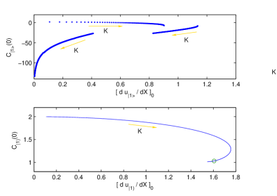
Figure 1: Upper plot: the “trajectory” $C_{|1\rangle}(0)$ vs $[du_{|1\rangle}/dX]_{0}$ for increasing $K$ values whithin the interval $[0,15]$ as indicated by the arrows. It is defined by the initial conditions of (1), or equivalently of (4-6). Lower plot: the corresponding “trajectory” defined by the initial conditions of the SP differential system (4), (6) and (7). The circle indicates the $\nu=\frac{1}{3}$ FQHE solution defined by (8). In both plots, the $K=0$ free-electron case is defined by the upper left point $[du/dX]_{0}=0$ and $C(0)=2$.

Equation (1) is linear and hence dispersive in its free-particle angular-momentum eigenspace. Its stationary solutions are expected to spread out over more and more eigenstates $|m\rangle$ when the perturbation defined by $K\neq 0$ grows. This is best illustrated by Fig. 1 (upper plot). Starting at $K=0$ (no interaction) from $m=1$ lowest-energy and most stable free-electron vortex state $|1\rangle$ defined by (1), it implicitely displays in terms of increasing $K$ the “trajectory” corresponding to the solution of (1) in its initial-condition phase space. Let us rewrite (1) under the form of the following equivalent differential system:

$$\Bigl{[}\nabla_{X}^{2}+C_{|1\rangle}-\frac{1}{X^{2}}-\frac{X^{2}}{4}\Bigr{]}u_{|1\rangle}=0,$$ (4)

$$\nabla_{X}^{2}C_{|1\rangle}=K\delta(X),$$ (5)

with

$$C_{|1\rangle}(X)=\mu_{|1\rangle}-{\cal W}_{|1\rangle}(X),$$ (6)

where $\delta(X)$ is the Dirac function, the radial Laplacian $\nabla_{X}^{2}$ is 3D in (5) while it remains 2D in (4) (this point will be discussed further below), the eigenvalue $\mu_{|1\rangle}$ stands for $E_{|1\rangle}+1$ due to the Larmor rotation at $m=1$ and ${\cal W}_{|1\rangle}=K/X$ describes the particle-particle interaction potential defined by the last term in (1). Then the initial-condition phase space becomes $C_{|1\rangle}(0)$ vs $[du_{|1\rangle}/dX]_{0}$. Indeed, we let $u(0)=[dC/dX]_{0}=0$ due to, respectively, complete depletion in the vortex trough and radial symmetry (no cusp). There are clearly two discontinuities in Fig. 1 (upper plot) which describe the “jumps” of the initial $m=1$ solution to higher orbital momenta when $K$ grows. In particular, there is a phase transition (infinite slope) at $[du_{|1\rangle}/dX]_{0}\sim 0.85$ and $C_{|1)}(0)\sim-7$. Now compare with Fig. 1 (lower plot). It displays the trajectory of the nonlinear Schrödinger-Poisson (SP) solution which is defined from (4-6) by adding the mean-field source term $u_{|1)}^{2}$ to Poisson equation (5), namely:

$$\nabla^{2}C_{|1)}=u_{|1)}^{2},$$ (7)

(we emphasize the eigenstate’s nonlinear nature imposed by Eq. (7) by using parentheses instead of kets).

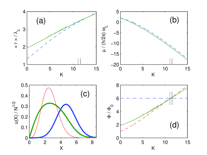
Figure 2: The nonlinear SP model for CF illustrated by its four basic properties. The experimental range (8) of nonlinearity $K$ is displayed by the two vertical marks. (a): the “nonlinear” radius ${\bar{X}}$ defined by (13) (continuous line) compared with ${\bar{Y}}$ defined by (14) (broken line). (b): the “nonlinear” eigenvalue $\mu_{|1)}$ defined by (4), (6) and (7) (continuous line) compared with $\mu_{|1\rangle}$ defined by (4-6) (broken line). (c): the FQHE normalized profiles $|1)$ (left: bold green) and $|1\rangle$ (right: bold blue) at $K={\cal N}_{|1)}=11.23$ (broken-line profiles in Fig. 3), compared with the modulus of Laughlin’s $\nu=\frac{1}{3}$ normalized wave function (9) (thin red line). (d): the “nonlinear” magnetic flux $\Phi_{|1)}$ given by (13) and (15) in continuous green line, compared with $\Phi_{|1\rangle}$ given by (14) and (15) in broken red line. The horizontal broken blue line at $\Phi/\Phi_{0}=6$ refers to (9) whose flux does not depend on $K$ and yields $6\Phi_{0}$ Laughlin (1987).

The spectral coherence of the new solution —i.e. the invariance of its angular momentum with respect to the increase of $K$— is obvious: instead of discontinuously spreading out in the momenta space like in Fig. 1 (upper plot), the SP solution starts spiraling down while keeping its $m=1$ initial value Reinisch and Gudmundsson (2012). No phase transition towards higher angular momenta occurs for $0\leq K\leq 15$ (e.g. in Fig. 1, lower plot, at $[du_{|1)}/dX]_{0}\sim 1.75$ and $C_{|1)}(0)\sim 1.3$).

This phenomenon resembles the well-known soliton coherence in hydrodynamics due to the cancellation of the dispersive effects by nonlinearity. The mathematical tool that explains the stability of the resulting solitary wave is the so-called nonlinear spectral transform. It provides a theoretical link between linear spectral —and nonlinear dynamical and/or structural properties of the wave Remoissenet (1999). This is what our nonlinear transformation from (5) to (7) is doing. It introduces an explicit ab-initio nonlinearity that cancels the angular-momentum dispersion displayed by Fig. 1 (incidently, this transformation is usually done the opposite way in classical soliton physics: one starts with the “real” nonlinear wave equation and ends up with its formal “spectral transformed” linear counterpart Remoissenet (1999)). As shown by Fig. 2a, the resulting nonlinear eigenstate $|1)$ defined by the SP differential system (4), (6) and (7) yields an average spatial extension which fits with the prediction of the linear equation (1) provided $K$ is chosen in the following FQHE experimental range defined by (2-3):

$$11.07\leq K=\frac{4\pi^{3/2}Mc^{2}}{\epsilon\Phi_{0}^{3/2}\sqrt{B}}=\kappa\frac{4\pi^{3/2}m_{e}c^{2}}{\epsilon\Phi_{0}^{3/2}}\leq 11.56.$$ (8)

This range of relevant $K$ values is indicated by the circle in Fig. 1 (lower plot) and by the two vertical marks in Figs 2a,b,d. Most important for the aim of the present letter, the nonlinear transformation from (5) to (7) yields the expected CF properties about gap stability and flux quantization (see Fig. 2b and 2d, respectively) while the spatial extension of the nonlinear eigenstate $|1)$ also agrees with Laughlin’s $\nu=\frac{1}{3}$ two-electron normalized wavefunction whose modulus $|\Psi_{3}|$ is derived from Chakraborty and Pietiläinen (1995):

$$\Psi_{3}\propto(z_{1}-z_{2})^{\displaystyle 3}\,e^{\displaystyle-\frac{(|z_{1}|^{2}+|z_{2}|^{2})}{4\lambda_{c}}}\propto X^{\displaystyle 3}e^{\displaystyle 3i\phi}e^{\displaystyle-\frac{X^{2}}{4}},$$ (9)

up to the unimportant factor $\exp[\frac{1}{2}({\bar{z}}/\lambda_{c})^{2}]$ related to the external degree of freedom. Figure 2c indeed displays the FQHE states defined by (8) (broken-line profiles in Fig. 3), namely $|1)$ (nonlinear: bold green) and $|1\rangle$ (linear: bold blue), as compared to normalized $|\Psi_{3}|$ (thin red).

The amplitude of the wavefunction defined by Eqs (4), (6) and (7) reads $\Psi_{|1)}=u_{|1)}\sqrt{M\omega_{L}/(\pi\hbar{\cal N}_{|1)})}$ where Reinisch and Gudmundsson (2012)

$${\cal N}_{|1)}=\int_{0}^{\infty}u_{|1)}^{2}XdX,$$ (10)

in order to achieve normalization according to $\int_{0}^{\infty}||\Psi_{|1)}(x,y)||^{2}dxdy=1$. Norm (10) is the nonlinear order parameter of our SP model Reinisch and Gudmundsson (2012). As it grows, the amplitude and width of $u_{|1)}$ increases while its corresponding normalized profile $u_{|1)}/\sqrt{{\cal N}_{|1)}}$ spreads out: see Fig. 3. Comparing the (last) interaction term of the bracket in (1) with the asymptotic solution

$$\lim_{X\rightarrow\infty}{\cal W}_{|1)}(X)={\cal N}_{|1)}G(X)$$ (11)

of (6-7) where the 3D Green function defined by (5) is $G(X)=X^{-1}$, we obtain:

$${\cal N}_{|1)}=K.$$ (12)

Equation (12) operates the link between the two-particle linear description (1) and the mean-field single-(quasi)particle provided by (4), (6) and (7). In Du et al. (1993) the filling factor $\nu=\frac{1}{3}$ lies at the intersection of two slopes concerning sample A. Taking their average, we obtain $K\sim 11.23$ which will be our reference value in interval (8). Note that it largely exceeds $K=\sqrt{2}$ in Laughlin (1983b). Similarly, ${\cal N}_{|1)}=11.23$ in accordance with (12) yields a strong nonlinearity: e.g. compare it with $2.53$ in quantum-dot helium Reinisch and Gudmundsson (2012). This is quite spectacularly illustrated by Fig. 3 where the linear solution $|1\rangle$ of (1) —or equivalently of system (4-6)— is compared with solution $|1)$ of the nonlinear SP system (4), (6) and (7) for increasing $K$ values. The profiles defined by $\nu=\frac{1}{3}$ FQHE value $K={\cal N}_{|1)}=11.23$ are displayed in broken lines: obviously they are strongly modified with respect to the free-particle ones (in dotted lines).

Let us now be specific about some technical points used in order to obtain the above results. In FQHE, the zeros of the Jastrow-type many-electron wave function proposed by Laughlin for odd polynomial degree look like 2D charges which repel each other by logarithmic interaction, yielding a negative value for the energy $E$ per electron Chakraborty and Pietiläinen (1995). Consequently we solve the Poisson equation (7) in 2D, which indeed ensures that the corresponding Green function becomes $G(X)=-\log(X)$. Therefore we obtain the “fully 2D” self-consistent SP differential system (4), (6) and (7) whose eigensolution $u_{|1)}(X)$ is defined by 8, (10) and (12).

The radius of SP’s nonlinear state $|1)$ displayed by Fig. 2a:

$${\bar{X}}=\sqrt{\langle{\bar{z}}^{2}\rangle}_{|1)}=\frac{1}{\sqrt{2}}[\langle X^{2}\rangle_{|1)}+\langle X\rangle^{2}_{|1)}]^{\frac{1}{2}},$$ (13)

is obtained from ${\bar{z}}=\frac{1}{2}(z_{1}+z_{2})$ by quantum-averaging $X$ and $X^{2}$ in the state $|1)$ (hence the subscripts) since the two electrons located at $z_{1}$ and $z_{2}$ are both in the same state $|1)$Griffiths (2005). On the other hand, $|z_{1}-z_{2}|$ is the diameter of the two-electron orbit defined by the linear internal degree of freedom $|1\rangle$ when assuming that the external degree of freedom ${\bar{z}}$ is frozen in its ground state. Therefore its radius:

$${\bar{Y}}=\frac{1}{2}\langle|z_{1}-z_{2}|\rangle_{|1\rangle}=\frac{1}{\sqrt{2}}\langle X\rangle_{|1\rangle}$$ (14)

(broken line in Fig. 2a ) can indeed be compared with (13) (continuous line). Like already emphasized, these two radii coincide at the experimental range (8) displayed by the couple of adjacent vertical marks in Fig. 2a.

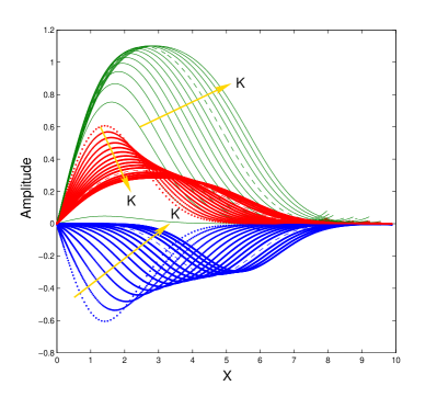
Figure 3: Left: The broadening and flatening of the normalized linear profile $-u_{|1\rangle}(X)/\sqrt{{\cal N}_{|1\rangle}}$ corresponding to eigenstate $|1\rangle$ of (4)-(6) (in bold blue and multiplied by $-1$ for the sake of clarity), compared with the normalized nonlinear SP wave function $u_{|1)}(X)/\sqrt{{\cal N}_{|1)}}$ of (4), (6) and (7) (in bold red) when ${\cal N}_{|1)}=K$ increases by integer steps from $0$ (free-electron solution: dotted profiles) to $15$. The SP solution $u_{|1)}(X)$ is displayed in green and increases with $K$. The CF profiles defined by ${\cal N}_{|1)}=K=11.23$ are displayed in broken lines.

The nonlinear energy eigenvalue $\mu_{|1)}$ solution of (4), (6) and (7) (continuous line in Fig. 2b ) is obtained from (6) by use of the 2D Green function $G(X)=-\log(X)$ either from the initial condition $C_{0}=C_{|1)}(0)$ with ${\cal W}_{|1)}(0)=\int_{0}^{\infty}G(X)u_{|1)}^{2}(X)dX$ in agreement with (7); or at the boundary $C_{|1)}(X\rightarrow\infty)$ by use of (11). The equivalence of these two definitions constitutes a test for the relevance of our numerical code: they fit within a relative error of $10^{-7}$. On tne other hand, the energy eigenvalue $\mu_{|1\rangle}$ corresponding to the solution $u_{|1\rangle}$ of the linear differential system (4-6) can also be obtained from (6) at the two above limits by simply using the explicit 2D definition ${\cal W}_{|1\rangle}(X)=-K\log(X)$. It is displayed in Fig. 2b by the broken line. The negative energy gap $\Delta=\mu_{|1)}-\mu_{|1\rangle}$ yields the stability of $|1)$ when compared with $|1\rangle$. Though small, it is clearly visible. We obtain at the experimental FQHE value $K=11.23$: $\mu_{|1\rangle}=-11.0807$ $\hbar\omega_{L}$ $=-0.6977$ $e^{2}/\epsilon\lambda_{c}$ and $\mu_{|1)}=-11.7164$ $\hbar\omega_{L}$ $=-0.7377$ $e^{2}/\epsilon\lambda_{c}$ (cf. (2)). Therefore $\Delta=-0.04$ $e^{2}/\epsilon\lambda_{c}$, to be compared with some experimental value $\Delta\sim-0.1$ $e^{2}/\epsilon\lambda_{c}$ Du et al. (1993). Moreover, the nonlinear eigenenergy per particle in our $N_{e}=2$ system is $E_{2}=\frac{1}{2}\mu_{|1)}=-0.37$ $e^{2}/\epsilon\lambda_{c}$. In the $20\leq N_{e}\leq 144$ interacting electron case in the disk geometry with the filling factor $\nu=\frac{1}{3}$, $E_{2}\sim-0.39$ $e^{2}/\epsilon\lambda_{c}$ by extrapolation to $N_{e}=2$ of the Monte Carlo evaluation of the ground-state energy per particle Morf and Halperin (1986). On the other hand, $E\sim-0.41$ $e^{2}/\epsilon\lambda_{c}$ per particle is almost insensitive to the system size for $4\leq N_{e}\leq 6$ Yoshioka et al. (1983). Therefore our $E_{2}=-0.37$ $e^{2}/\epsilon\lambda_{c}$ seems quite acceptable in this context.

Figure 2d displays the fundamental property of the present model, namely, its $6\Phi_{0}$ flux quantization for the LLL filling factor $\nu=\frac{1}{3}$ in the experimental range defined by 8. Indeed we have respectively from (13) and (14):

$$\frac{\Phi_{|1)}}{\Phi_{0}}=\frac{\pi B\lambda_{c}^{2}}{\Phi_{0}}\,{\bar{X}}^{2}=\frac{1}{2}{\bar{X}}^{2}=6,$$ (15)

$$\frac{\Phi_{|1\rangle}}{\Phi_{0}}=\frac{\pi B\lambda_{c}^{2}}{\Phi_{0}}\,{\bar{Y}}^{2}=\frac{1}{4}\langle X\rangle_{|1\rangle}^{2}=6,$$ (16)

between the two vertical marks. The (blue) horizontal broken line at $\Phi/\Phi_{0}=6$ refers to Laughlin’s $\nu=\frac{1}{3}$ normalized wavefunction ansatz (9) which does not depend on $K$. Its flux is indeed $6\Phi_{0}$ Laughlin (1987)).

In conclusion, we stress the self-consistency of our FQHE nonlinear model. The spectral coherence of the mean-field SP mode $|1)$ slightly lowers the energy per electron with respect to that obtained from Schrödinger’s two-electron internal mode $|1\rangle$. This gap makes the nonlinear mode $|1)$ energetically favourable for the fulfilment of the flux quantization condition (15) than the linear SP mode $|1\rangle$ for (16). This property might be considered as the attachment of two flux quanta per electron and the subsequent transformation of this later into a nonlinear soliton-like CF whose 3rd remaining flux quantum makes it behave as a mere quasiparticle in LLL Integral Quantum Hall Effect.