Reaction Spreading on Percolating Clusters

Abstract

Reaction diffusion processes in two-dimensional percolating structures are investigated. Two different problems are addressed: reaction spreading on a percolating cluster and front propagation through a percolating channel. For reaction spreading, numerical data and analytical estimates show a power law behaviour of the reaction product as $M(t)\sim t^{d_{\scriptsize{\mbox{l}}}}$, where $d_{\scriptsize{\mbox{l}}}$ is the connectivity dimension. In a percolating channel, a statistically stationary travelling wave develops. The speed and the width of the travelling wave are numerically computed. While the front speed is a low-fluctuating quantity and its behaviour can be understood using simple theoretical argument, the front width is a high-fluctuating quantity showing a power-law behaviour as a function of the size of the channel.

I Introduction

Reaction diffusion processes have been extensively studied in the past years as systems able to shed some light on various problems of different disciplines Murray ; Peters . Recently, the importance of the non-homogeneity of the medium over which the reaction and diffusion take place has been highlighted Porto1997 , since the qualitative and quantitative features of the spreading of the reaction process can depend on the presence of system irregularities. Many studies in the last years concern reaction/diffusion process in heterogeneous media accomplishing different problems spacing from epidemic evolution in heterogeneous networks Vespignani2007 , or the intracellular calcium dynamics Thul2004 to the combustion in porous media Tarta2008 . In this context, studies on reaction dynamics on percolating clusters appear very interesting for their physical relevance and their applications in many different scientific and technological fields Degennes ; cardy ; Hav ; isich . For recent experimental and numerical results for reaction-diffusion on heterogeneous media, see Sol_1 ; Sol_2 ; Gor_11 ; Marin ; Das ; Atis

The study of reaction and diffusion dynamics on homogeneous substrate date back to the Fisher-Kolmogorov-Petrovskii-Piskunov (FKPP) model FKPP

$$\partial_{t}\theta=D\Delta\theta+\alpha g(\theta)\,,$$ (1)

where the scalar field $\theta$ represents the fractional concentration of the reaction products, $D$ is the molecular diffusivity, $g(\theta)$ describes the reaction process and $\alpha$ is the reaction rate, i.e., the inverse of the characteristic time, $\tau$, of the reaction process. In the original model FKPP $g(\theta)$ assumes a convex shape $g(\theta)=\theta(1-\theta)$. It is possible to show that under very general conditions FKPP , i.e. if $g(\theta)$ is a convex function and $g^{\prime}(0)=1$, a travelling wave develops with asymptotic speed and width given by

$$v_{0}=2\sqrt{\alpha D},\,\,\,\,\,\,\,\delta_{0}=c\sqrt{D/\alpha}$$

where the constant $c$ depends on the definition adopted for the computation of the front width.
Afterward, as previously mentioned, reaction-transport dynamics attracted a considerable interest for their relevance in an incredible large number of chemical, biological and physical systems Murray ; Peters . In general, when dealing with a non trivial environment for the reaction and diffusion process it is possible to extend Eq. (1) in order to take into account the properties of the medium acvv01 ; Mancinelli ; bcvv2012 :

$$\partial_{t}\theta=\hat{L}\theta+f(\theta)\,\,,$$ (2)

where the linear operator $\hat{L}$ rules the transport process. An important class of processes of this type is the advection-reaction-diffusion processes, where $\hat{L}=-\mathbf{u}\cdot\mathbf{\nabla}+D\Delta$ (e.g., see acvv01 ). On the other hand it is possible to extend the $\hat{L}$ operator in order to include cases of effective diffusion on fractal objects $\hat{L}=\frac{1}{r^{d_{\scriptsize{\mbox{f}}}-1}}\frac{\partial}{\partial r}\left(k(r)r^{d_{\scriptsize{\mbox{f}}}-1}\frac{\partial}{\partial r}\right)$ Procaccia1985 suitable to study reaction dynamics on fractals Mendez2010 . Moreover in a recent paper bcvv2012 , the reaction spreading on graphs has been considered; in such a case, the operator $\hat{L}$ is nothing but the Laplacian operator for graphs bollobas1998 ; bc05 . In the present paper, in the spirit of the cited works, we study reaction and diffusion dynamics on percolation clusters, considering the spreading properties of such a process.
In Sect. 2 we present the model and some numerical details. Sect. 3 is devoted to the study of reaction spreading in a large percolating cluster, while front propagation in a percolating channel is discussed in Sect. 4. In Sect. 5 the reader can find some conclusions.

II Model

A natural model to study reaction and diffusion on a two dimensional non homogeneous medium can be constructed starting from a generalization of Eq. (1) in which the transport operator, $\hat{L}=D({\mathbf{x}})\Delta$, depends on the spatial variable:

$$\partial_{t}\theta({\mathbf{x}},t)=D({\mathbf{x}})\Delta\theta({\mathbf{x}},t)+f(\theta({\mathbf{x}},t))\,.$$ (3)

The shape and the spatial distribution of $D({\mathbf{x}})$ permits to take into account the properties of the medium and therefore to consider different physical and biological topics SK_97 ; OL_01 . In this way it is possible to study the reaction dynamics at the “microscopic” level without assuming any effective equation able to incorporate mainly qualitative features of the heterogeous medium Procaccia1985 ; Mendez2010 ; Alonso2009 .
Since we are mainly interested on the scaling properties of the asymptotic behaviour of the system, without weakening the results we consider the case in which the variable $D(x)$ can assume only two values, i.e., $D(x)=0$ in forbidden spatial regions and $D(x)=D_{0}$ in permitted ones. The second step is to consider a spatial discretization of Eq. (3). The spatial region under examination has been discretized using a 2d Euclidean lattice, $\mathcal{L}$, where $\Delta x$ is the lattice constant. Points ${\mathbf{x}}$ are replaced by sites of the lattice $s=(i,j)$.

The percolating clusters have been obtained as follows. Each site may be permitted (with probability $p$) or prohibited (with probability $1-p$). If $p>p_{c}$, where $p_{c}\simeq 0.592746$ is the site percolation threshold for square lattices, there is a good chance that the reaction, starting from any of the permitted sites can invade the system (percolation). We call $\mathcal{P}$ the set of the permitted sites. In each permitted site we have a value of the concentration field, $\theta_{s}(t)=\theta_{(i,j)}(t)$. Eq (3) can be discretized as follows

$$\frac{\mathrm{d}}{\mathrm{d}t}\theta_{s}=\sum_{s^{\prime}}C_{s,s^{\prime}}\theta_{s^{\prime}}+f(\theta_{s})\,,$$ (4)

where $\sum_{s^{\prime}}C_{s,s^{\prime}}\theta_{s^{\prime}}$ is the discretization of the general transport operator $\hat{L}=D(x)\Delta\theta({\mathbf{x}},t)$. Since we are working on a discrete structure the value of the lattice spacing $\Delta x$ is not particularly important (it can be “absorbed” in $D_{0}$ for $D_{0}$ and $\delta_{0}$ large enough), therefore we assume $\Delta x=1$.

In order to specify the quantity $C_{s,s^{\prime}}$ we introduce the variable $A_{s}$ that characterizes the permitted region of the lattice:

$$A_{s}=\left\{\begin{array}[]{cl}1&{\rm if}\ s\in\mathcal{P}\cr 0&{\rm if}\ s\not\in\mathcal{P}\cr\end{array}\right.$$ (5)

Given a site $s$ we can define $k_{s}=\sum_{|s^{\prime}-s|=1}A_{s^{\prime}}$ as the number of permitted nearest neighbors of $s$. Using these quantities and imposing the mass conservation of the diffusion operator, we can express $C_{s,s^{\prime}}$ as

$$C_{s,s^{\prime}}=D_{0}\left\{\begin{array}[]{ll}0&{\rm if}\,\,\,\,|s-s^{\prime}|>1\cr A_{s^{\prime}}&{\rm if}\,\,\,\,|s-s^{\prime}|=1\cr k_{s}&{\rm if}\,\,\,\,s=s^{\prime}\end{array}\right.$$ (6)

So that, the discretized transport term $\hat{L}\theta_{s}=\sum_{s^{\prime}}C_{s,s^{\prime}}\theta_{s^{\prime}}$ becomes the discrete Laplacian of the lattice bollobas1998 :

$$\hat{L}\theta_{s}(t)=D_{0}\left(\sum_{|s^{\prime}-s|=1}\left(A_{s^{\prime}}\theta_{s^{\prime}}(t)\right)-k_{s}\theta_{s}(t)\right)$$ (7)

Finally, the complete model of reaction diffusion on percolating clusters reads

$$\frac{\mathrm{d}}{\mathrm{d}t}\theta_{s}=D_{0}\left(\sum_{|s^{\prime}-s|=1}\left(A_{s^{\prime}}\theta_{s^{\prime}}(t)\right)-k_{s}\theta_{s}(t)\right)+\alpha g(\theta_{s})\,\,,$$ (8)

where, following classical works FKPP we choose $f(\theta)=\alpha g(\theta)$ where $g(\theta)=\theta_{s}(1-\theta_{s})$. From the numerical viewpoint, given the spatial discretization, the temporal derivative is computed via a 4-th order Runge-Kutta algorithm.

In the following we study two different problems. The first concerns reaction spreading on a large 2d percolating cluster without a specific geometry (see Figure 1), and starting from an initial condition $\theta_{s}(0)=0$ except a single site, $\tilde{s}$, in which $\theta_{\tilde{s}}(0)=1$. In the second problem we study the front propagation features (speed and width of the travelling wave) in a 2d channel with dimensions $L_{x}\times L_{y}$ with $L_{x}\geq L_{y}$ (see Figure 3). In the numerical computations, the lattice is dynamically modified in order to follow the reacting front, i.e., the domain considered in the computation moves rigidly downstream when in the upstream part the reaction is extinguished. In all the simulations, without lack of generality, we fix $D_{0}=1$.

It is worth saying that, for $p<p_{c}$, the propagation is practically forbidden if the system is very large. For finite systems one has yet a possible propagation if $p$ is not much lower than $p_{c}$, as can be seen in the following (in particular in Fig 4).

III Reaction spreading

An important quantity that characterizes the spreading of the reaction is the total mass of the reaction product, i.e., $M(t)=\sum_{s\in\mathcal{P}}\theta_{s}(t)\,.$

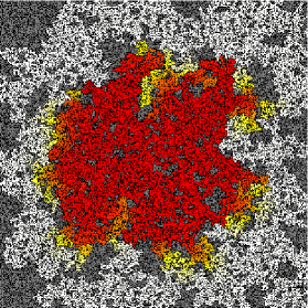
Figure 1: Reaction spreading on a square lattice (color online). The red area contains reaction products, the yellow area is the one where the reaction takes place, and the white area contains fresh material. The black dots indicate prohibited sites, whereas the various grey areas indicate regions of permitted sites that do not belong to the percolating cluster (we call them islands).

Since this quantity depends on the number of permitted sites, we introduce the percentage of $m(t)$ over the lattice, i.e.,

$$m(t)=\frac{M(t)}{N}=\frac{\displaystyle{\sum_{s\in\mathcal{P}}\theta_{s}(t)}}{\displaystyle{\sum_{s\in\mathcal{L}}A_{s}}}$$ (9)

where $N=\sum_{s\in\mathcal{L}}A_{s}=\sum_{s\in\mathcal{P}}1$ is the number of permitted sites.

Let us briefly remind some relevant quantities in the statistical analysis of generic graphs: the fractal dimension, $d_{\scriptsize{\mbox{f}}}$, the connectivity dimension, $d_{\scriptsize{\mbox{l}}}$, (also called chemical dimension) and the spectral dimension, $d_{\scriptsize{\mbox{s}}}$. The fractal dimension $d_{\scriptsize{\mbox{f}}}$ ccv describes the scaling of the number of permitted sites in a sphere of radius $r$ in the lattice, as ${\mathcal{N}}(r)\sim r^{d_{\scriptsize{\mbox{f}}}}$. The connectivity dimension, instead, measures the average number of sites connected to a given site in at most $l$ step, as ${\mathcal{N}}(l)\sim l^{d_{\scriptsize{\mbox{l}}}}$. The spectral dimension is related to diffusion processes on graphs and can be defined in terms of the return probability $P_{ii}$ at site $i$ for a random walker by $P_{ii}(t)\sim t^{-d_{\scriptsize{\mbox{s}}}/2}$, or equivalently in terms of the density of eigenvalues of the Laplacian operator bc05 . The connectivity and fractal dimension can be obviously different and they are related via the mapping between the two distances $r$ and $l$ Havlin1984 . In particular for site percolation in square lattices, the case of the present study, at percolation threshold $p\sim p_{c}$ one has $d_{\scriptsize{\mbox{f}}}\simeq 1.896$ but $d_{\scriptsize{\mbox{l}}}\simeq 1.67$ (and, for completeness, $d_{\scriptsize{\mbox{s}}}\simeq 1.36$).

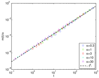
Figure 2: Time evolution at $p=0.595\approx p_{c}$ of the percentage of the quantity of products rescaled by $\alpha$, $m(t)/\alpha$ vs $t$, together with the prediction $m(t)/\alpha\simeq t^{d_{\scriptsize{\mbox{l}}}}$ with $d_{\scriptsize{\mbox{l}}}\simeq 1.67$ (dashed line). In order to get smooth quantities, $m(t)$ is averaged over many realizations ($\approx 5000$) of lattices of size $L_{x}=1000$ and $L_{y}=1000$ which are portions of larger lattices.

Which is the right quantity that characterizes the reaction spreading? Numerical computations in agreement with analytical arguments bcvv2012 suggest that the chemical dimension is the right quantity. Starting from a single site with $\theta_{i}(0)=1$, after $t$ step the number of site reached by the field is ${\mathcal{N}}(t)\sim t^{d_{\scriptsize{\mbox{l}}}}$ Grass . Therefore, in the limit of very fast reaction, when each site reached by the field is immediately burnt (i.e, $\theta_{s}\simeq 1$), we can expect:

$$m(t)\sim t^{d_{\scriptsize{\mbox{l}}}}.$$ (10)

Fig. 2 clearly shows the scaling of Eq. (10). Moreover this Figure reveals that the scaling (10) is valid not only in the fast reaction regime, and that the reaction rate is relevant only for the prefactor: $m(t)\simeq\alpha t^{d_{\scriptsize{\mbox{l}}}}$.

IV Front propagation

The problem of the front propagation in reactive systems (classical reaction and diffusion processes, advection reaction and diffusion processes, reaction and diffusion in the presence of anomalous diffusion, etc.) has been extensively studied Murray ; Peters ; Mancinelli . In some cases, under certain conditions, it is possible to show that the propagation is standard, i.e., there exists an asymptotic value for the speed $v$ and the width $\delta$ of the propagating front. On the other hand, it is pretty impossible (except very special cases) to determine analytically the values of $v$ and $\delta$. Therefore the numerical study of the speed and the thickness of the moving front is mandatory to obtain information about the spreading dynamics.

In the case of reaction processes on percolating clusters, if one considers an arbitrarily large (in any direction) lattice, the propagation generally is not standard since the total quantity of reaction products grows as a power law with a non integer exponent, $m(t)\simeq\alpha t^{d_{\scriptsize{\mbox{l}}}}$. If the percolating cluster is embedded in a channel with a propagation direction, $L_{x}$, and a transversal direction, $L_{y}$, with $L_{x}\geq L_{y}$, a travelling wave takes place with a constant (on average) speed after a transient needed to the reaction product to invade the transversal direction of the channel. Therefore, we consider the model (8) with an initially empty 2d lattice where $L_{x}\geq L_{y}$ and $\theta_{(i,j)}(0)=0$. In order to reduce the transient, as boundary conditions we use $\theta_{(i=0,j)}(t)=1$ and $\theta_{(i=L_{x},j)}(t)=0$ for the left and right edge, respectively. In the transversal direction we have zero-flux (Neumann) boundary conditions, that are automatically guaranteed by the diffusion operator (7). Using the above boundary conditions, we expect the development of a front propagating with a fixed (on average) speed from the left to the right side of the lattice.

In Fig. 3 it is shown an example of front propagation in a percolating cluster. The dynamic evolves through the horizontal direction with a fluctuating front depending on the position of the permitted sites. Because of such fluctuations it is convenient to introduce the averaged field along the horizontal direction as the mean of the field $\theta_{s}(t)$ along the $i$-direction

$$\theta_{i}(t)=\frac{\displaystyle{\sum_{j=1}^{L_{y}}A_{(i,j)}\theta_{(i,j)}(t)}}{\displaystyle{\sum_{j=1}^{L_{y}}A_{(i,j)}}}.$$ (11)

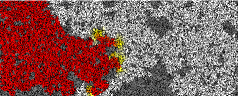
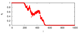
Figure 3: Snapshot of the reaction dynamics in a percolating cluster on a channel (color online, see caption of Figure 1). The graph below shows the profile of the average of the front (see Eq. (11)) related to the snapshot.

Strictly speaking, given a percolating cluster, the moving front is not a travelling wave in the classical sense, since there does not exist a function $f(i)$ such as $\theta_{i}(t)=f(i-vt)$. This is due both for the random nature of the permitted sites on the lattice (i.e., the average stabilizes only at very large $L_{y}$) and for the discrete nature of the lattice. But it is still possible to define averaged quantities such as the propagation speed or the front width as follows.

IV.1 Front speed

In the case of travelling waves, we expect that the total mass of the reaction products increases, on average, linearly with time

$$M(t)\simeq N_{p}vt$$ (12)

where $N_{p}$ is the averaged number of site accessible by the reaction process in the vertical direction. The computation of $N_{p}$ is a quite delicate point thus the maximum amount of accessible sites in a single column of the lattice is not $L_{y}$ (since there are permitted and prohibited site in the lattice) neither $pL_{y}$ (since not the whole set of permitted sites belong to the percolating cluster). $N_{p}$ can be estimated as follows. At the percolating threshold, $p\sim p_{c}$, the total number of points belonging to the percolating cluster in a square of size $L_{y}$ is proportional to $L_{y}^{d_{\scriptsize{\mbox{f}}}}$. Since there are $L_{y}$ rows in the square one has $N_{p}\sim\frac{L_{y}^{d_{\scriptsize{\mbox{f}}}}}{L_{y}}=L_{y}^{d_{\scriptsize{\mbox{f}}}-1}$. Instead, if $p$ is large enough to have one single big percolating cluster, without the presence of closed islands of permitted sites not connected to the principal percolating cluster, one has $N_{p}\simeq pL_{y}$. In the intermediate cases it is possible to compute $N_{p}$ numerically. Therefore, we can define the average front speed as

$$v_{1}=\lim_{t\to\infty}\frac{M(t)}{N_{p}t}\,.$$ (13)

Another way to define $v$, that is much more sensitive to statistical fluctuations of the cluster structure, can be obtained starting from the dynamics of the model. Since the diffusion operator (7) is a mass-preserving term, the derivative of the total mass can be computed using Eq. (8)

$$v_{2}(t)=\frac{1}{N_{p}}\frac{{\mathrm{d}}}{{\mathrm{d}}t}M(t)=\frac{\alpha}{N_{p}}\sum_{s\in\mathcal{P}}(\theta_{s}(t)(1-\theta_{s}(t)))\,.$$ (14)

Of course $v_{2}(t)$ is a function of time and its fluctations reflect the random nature of the percolating cluster. On the other hand, we expect, as confirmed from numerical simulation (not shown), that $\langle v_{2}(t)\rangle=v_{1}=v_{\scriptsize{\mbox{f}}}$.

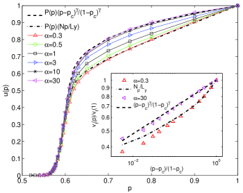
Figure 4: Average front speed $u(p)$ as a function of $p$ for various $\alpha$ together with asymptotic behaviour (15) and (16) (with $\gamma\simeq 0.16$). The channel length is taken to be $L_{x}=100$ and $L_{y}=100$. In the inset it is shown in log-log scale the behaviour of $v_{\scriptsize{\mbox{f}}}(p)/v_{\scriptsize{\mbox{f}}}(1)$ together with the theoretical prediction: $v_{\scriptsize{\mbox{f}}}(p)/v_{\scriptsize{\mbox{f}}}(1)\sim N_{p}/L_{y}$ for slow reaction rate and $v_{\scriptsize{\mbox{f}}}(p)/v_{\scriptsize{\mbox{f}}}(1)\sim((p-p_{c})/(1-p_{c}))^{\gamma}$ for fast reaction rate.

It is interesting to study the behaviour of $v_{\scriptsize{\mbox{f}}}$ as a function of $p$, the probability of having a permitted site. In fact, using different values of $p$ it is possible to model different degree of non-homogeneity and we expect different evolution of the reaction process. For $p=1$, since the lattice is homogeneous, we expect to obtain the FKPP value $v_{0}=2\sqrt{\alpha D_{0}}$. This result is true for small $\alpha$, when $\delta_{0}\sim\sqrt{D_{0}/\alpha}$ is larger than the lattice size (simulations not shown for the sake of brevity). On the contrary for large $\alpha$, because of the discrete nature of the lattice, the width of the FKPP front can be of the same order, or even smaller, of the lattice step. In this case there is a significant difference between the measured front speed and the FKPP value also for $p=1$. Although this discrepancy does not invalidate our analysis, we choose to study only rescaled velocity $v_{\scriptsize{\mbox{f}}}(p)/v_{\scriptsize{\mbox{f}}}(1)$.

In the case of $p<1$, especially for $p\sim p_{c}$, it is important to introduce the probability of having a percolating lattice, $P(p)$. We write $u(p)=P(p)v_{\scriptsize{\mbox{f}}}(p)/v_{\scriptsize{\mbox{f}}}(1)$ as the average velocity in a percolating cluster when the site probability is $p$. For value of $p$ larger than $p_{c}$ it is possible to give simple but valid arguments to explain the behaviour of $u$. First of all, for small $\alpha$ values we expect a large front that regularizes the propagation. This is a kind of homogenization regime acvv01 . Practically, we can imagine the front proceeding almost as in a homogeneous medium excluding the region in which the propagation is prohibited. Therefore we can write

$$u(p)=P(p)\frac{v_{\scriptsize{\mbox{f}}}(p)}{v_{\scriptsize{\mbox{f}}}(1)}\sim P(p)\frac{N_{p}}{L_{y}}\,.$$ (15)

Such a relation, when $p$ is large, simplifies to $v_{\scriptsize{\mbox{f}}}(p)\sim pv_{\scriptsize{\mbox{f}}}(1)$.

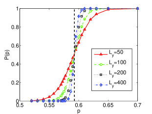
Figure 5: The probability $P(p)$ to percolate along a channel of size $L_{x}=L_{y}$ is shown for different $L_{y}$.

In the other limit, for large $\alpha$, we can use the following argument Havlin2000 . We know (from Eq. (10)) that $m(t)\sim t^{d_{\scriptsize{\mbox{l}}}}$. On the other hand $m(t)\sim r(t)^{d_{\scriptsize{\mbox{f}}}}$. Therefore $r(t)\sim t^{d_{\scriptsize{\mbox{l}}}/d_{\scriptsize{\mbox{f}}}}$, and $v=\frac{dr}{dt}\sim t^{d_{\scriptsize{\mbox{l}}}/d_{\scriptsize{\mbox{f}}}-1}\sim r^{1-d_{\scriptsize{\mbox{min}}}}$, where $d_{\scriptsize{\mbox{min}}}=\frac{d_{\scriptsize{\mbox{f}}}}{d_{\scriptsize{\mbox{l}}}}$. Furthermore, if the linear size of the region is $r<\xi$, where $\xi$ is the correlation length Hav , the cluster is self-similar and then $v\sim\xi^{1-d_{\scriptsize{\mbox{min}}}}$. Moreover, analysis of the percolation phase transition gives $\xi\sim|p-p_{c}|^{-\nu}$, with $\nu=4/3$ for $d=2$ den , which gives the final scaling $v\sim(p-p_{c})^{\gamma}$, where $\gamma=-\nu(1-d_{\scriptsize{\mbox{min}}})$. For the average velocity, the scaling is:

$$u(p)=P(p)\frac{v_{\scriptsize{\mbox{f}}}(p)}{v_{\scriptsize{\mbox{f}}}(1)}\sim P(p)\left(\frac{p-p_{c}}{1-p_{c}}\right)^{\gamma}.$$ (16)

Alternatively, a similar scaling had been derived through large deviation theory Mendez2010 . Both the above behaviors are well observed in the numerical simulations, as shown in Fig. 4. It is worth noting that below the percolation threshold, the probability to have a percolating cluster tends to zero for a channel long enough, see Fig 5. Nonetheless, in Fig 4, it is possible to observe a very small velocity $u(p)$ for $p\lesssim p_{c}$. This result is basically due to the fact that, for finite size, $P(p)$ is not strictly zero for $p\lesssim p_{c}$, see Fig 5.

Concerning the probability $P(p)$ of having a percolating lattice as a function of $p$, in the numerical simulations it is possible to compute $P(p)$ only for finite values of $L_{x}$ and $L_{y}$. Moreover, in applications the cluster size is finite, and $L_{y}$ can be small. Fig. 5 shows $P(p)$ for different values of $L_{y}$ in the case of $L_{x}=L_{y}$. Naturally for $L_{y}\rightarrow\infty$, $P(p)$ approaches the Heaviside step function $\Theta(p-p_{c})$. Simulations (not reported here) show that for non square lattices $L_{x}=nL_{y}$ with $n>1$, while the front speed $v_{\scriptsize{\mbox{f}}}$ does not change with $n$, the probability $P(p)$ is strongly influenced by $n$, if $n$ is large. Moreover, in the case of large $n$, also $p_{c}$ changes, becoming dependent on both $n$ and $L_{y}$.

IV.2 Front width

For a two dimensional propagating wave in random media, we can define various different measure of width. One important measure concerns the averaged width of the front along the propagation direction. It is the analougous to the front width in the 1d FKPP traveling wave and measures the region along the x direction in which the reaction process is active (see Figure 3). In order to define such a quantity one can use $\theta_{i}(t)$, i.e. the average over the $i$-direction of the field $\theta_{s}(t)$, defined in Eq. (11). Yet the averaged quantity $\theta_{i}(t)$ still suffers from large fluctuation so we use a simplified observable able to give a good measure of the front width. First of all we introduce an auxiliary quantity

$$H_{(i,j)}(t)=\left\{\begin{array}[]{ll}1&{\rm if}\,\,\,\,0.01\leq\theta_{(i,j)}(t)\leq 0.99\cr 0&{\rm elsewhere}\end{array}\right.\,.$$ (17)

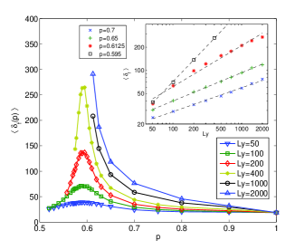
Figure 6: Averaged front width, $\langle\delta_{\scriptsize{\mbox{f}}}\rangle$, as a function of $p$ at varying $L_{y}$, where the horizontal size of the lattice is $L_{x}=5000L_{y}$. For all curves, $\alpha=1$. In the inset it is shown, for fixed values of $p$, the scaling behaviour of $\langle\delta_{\scriptsize{\mbox{f}}}\rangle\sim L_{y}^{\beta}$, where $\beta=0.94$ for $p=0.595$, $\beta=0.54$ for $p=0.6125$, $\beta=0.37$ for $p=0.65$, $\beta=0.31$ for $p=0.7$.

Then we define $\delta_{\scriptsize{\mbox{f}}}(t)$, the front width, as the distance between the maximum and the minimum value of $i$ such that $H_{(i,j)}(t)=1$. In this way we define a rectangle of size $L_{y}\,\times\,\delta_{\scriptsize{\mbox{f}}}(t)$ inside which there is the whole active front. Also $\delta_{\scriptsize{\mbox{f}}}(t)$ is a strongly fluctuating quantity, therefore we study the statistical feature of $\delta_{\scriptsize{\mbox{f}}}(t)$, e.g., $\langle\delta_{\scriptsize{\mbox{f}}}\rangle$, as a function of $p$ and $L_{y}$.

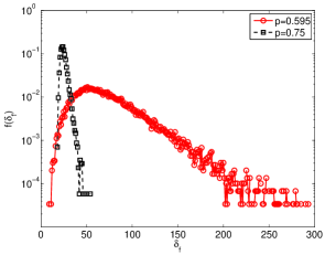
Figure 7: Two different probability density functions of ${\delta_{\scriptsize{\mbox{f}}}}$ for two values of p are shown: $p=0.595\approx p_{c}$ and $p=0.75$, with $L_{y}=100$, $L_{x}=5000L_{y}$ and $\alpha=1$. It is well evident that for $p\approx p_{c}$, fluctuations play a dominant role and large deviations are present.

In principle one can expect that given $p$ and $\alpha$, for $L_{y}$ large enough, the front width reaches a constant value, as for the front speed. On the other hand, as shown in Figure 6, the convergence depends on $p$: while for large $p$ (near to $p=1$) there is an asymptotic value of $\langle\delta_{\scriptsize{\mbox{f}}}\rangle$, for values of $p$ going to $p_{c}$ there is no convergence at all. Notably, in the limit of very large clusters, the averaged front width diverges rapidly around $p\sim p_{c}$. As the inset of Fig. 6 shows, the scaling structure of the front width as a function of $L_{y}$ at varying $p$ is highly non trivial and cannot be associate to a single scaling exponent Gross1 .

Rather interesting is the presence of very large fluctuations of $\langle\delta_{\scriptsize{\mbox{f}}}\rangle$. Fig. 7 shows how, for $p$ near $p_{c}$, the typical value of the front width, ${\delta_{\scriptsize{\mbox{f}}}}^{T}$, given by the maximum of the probability density function, is of the same order of the fluctuation of $\langle\delta_{\scriptsize{\mbox{f}}}\rangle$ (measured as $\sqrt{\langle\delta_{\scriptsize{\mbox{f}}}^{2}(t)\rangle-\langle\delta_{\scriptsize{\mbox{f}}}(t)\rangle^{2}}$).

The above discussion is valid at fixed (and not too small) $\alpha$. When $\alpha$ is small, the bare FKPP front width, $\delta_{0}$, is large, and a large front width regularizes the reaction dynamics. If the bare front width is larger than the typical size of the prohibited islands (for a given $p$) we can expect that the random distribution of the islands does not affect too much the front propagation, with a net effect of diminishing the fluctuations and the dependence of the front on both $p$ and $L_{y}$. On the other hand, for large $\alpha$ the bare front width is comparable with the lattice discretization. In this case fluctuations become very strong as the dependency of the front width both from $p$ and $L_{y}$. Figure 8 explicates the above discussion.

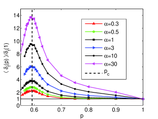
Figure 8: Normalised averaged front width for different values of the reaction rate with $L_{y}=100$, $L_{x}=5000L_{y}$. For small values of $\alpha$ fluctuations are smoothed, whereas they are maximal for large reaction rates.

V Conclusion

Reaction and diffusion processes in heterogeneous media, because of their relevance in many real-world applications, play a central role in several different fields. In the present paper, starting from the basic equations, we have investigated the behaviour of a simple reaction and diffusion process taking place in a heterogeneous medium, i.e., two-dimensional percolating structures. We show that for the reaction spreading on percolating clusters the dynamics is ruled by the connectivity dimension, $d_{\scriptsize{\mbox{l}}}$ (see Eq. (10)) and the reaction rate affects only the prefactor of the scaling. In the case of percolating clusters through a channel, the reaction and diffusion process develops a statistically stationary travelling wave. The speed and the width of the travelling wave are deeply influenced by the percolating transition together with finite size effects that generate peculiar behaviours of both front speed and front width. Those effects are crucial since, in realistic problems, the channel over which the reaction takes place has necessarily a finite transversal length. Some recent numerical computations and experiments show the key role played by the flow heterogeneities on the chemical front dynamics Gor_11 ; Marin ; Das ; Atis .

VI Acknowledgements

We thank R. Burioni for fruitful discussions.

References

- (1) J.D. Murray, Mathematical Biology, (Springer-Verlag, Berlin, 1993).
- (2) N. Peters, Turbulent combustion (Cambridge University Press, New York, 2000).
- (3) M. Porto, A. Bunde, S. Havlin, and H.E. Roman, Phys. Rev. E 56, 1667 (1997).
- (4) V. Colizza and A. Vespignani, Phys. Rev. Lett. 99, 148701 (2007).
- (5) R. Thul and M. Falcke, Phys. Rev. Lett. 93, 188103 (2004).
- (6) A. M. Tartakovsky, D. M. Tartakovsky, T. D. Scheibe, and P. Meakin, SIAM J. Sci. Comput., 30 2799 (2008).
- (7) P.G. de Gennes, La Recherche, 7, 919, (1976); P.G. de Gennes, J. Phys. Lett., Paris 37, L1, (1976).
- (8) J. L. Cardy and P. Grassberger, J. Phys. A: Math. Gen. 18, L267 (1985).
- (9) A. Bunde and S. Havlin, Fractals and Disordered Systems, Springer-Verlag Berlin (1999); S. Havlin and D. ben-Avraham, Advances in Physics, 36, 695 (1987).
- (10) M. B. Isichenko, Reviews of Modern Physics 64, 961 (1992).
- (11) M. S. Paoletti, and T. H. Solomon EPL, 69, 819 (2005).
- (12) M. E. Schwartz and T. H.Solomon, Phys. Rev. Lett., 100, 028302 (2008).
- (13) S Goroshin, F-D Tang, and A. J. Higgins, Phys.Rev. E 84, 027301(2011).
- (14) À. G. Marín, H. Gelderblom, D. Lohse, and J. H. Snoeijer, Phys. Rev. Lett., 107, 085502 (2011).
- (15) S Das, S Chakraborty, and S.K. Mitra, Phys. Rev. E 85, 046311 (2012)
- (16) S Atis, S Saha, H Auradou, D Salin, and L Talon, Phys. Rev. Lett., 110, 148301 (2013).
- (17) A. N. Kolmogorov, I. G. Petrovskii, and N. S. Piskunov, Moscow Univ. Bull. Math. 1, 1 (1937); R. A. Fischer, Ann. Eugenics 7, 355 (1937).
- (18) M. Abel, A. Celani, D.Vergni and A. Vulpiani, Phys. Rev. E 64, 046307 (2001).
- (19) R. Mancinelli, D. Vergni and A. Vulpiani, Physica D 185, 175 (2003).
- (20) R. Burioni, S. Chibbaro, D.Vergni and A. Vulpiani, Phys. Rev. E 86, 055101 (2012).
- (21) B. O’Shaughnessy, I. Procaccia, Phys. Rev. Lett. 54, 455 (1985); L. P. Richardson, Proc. R. Soc. London A 110, 709 (1926).
- (22) V. Mendez, D. Campos and J. Fort, Phys. Rev. E 69, 016613 (2004); D. Campos, V. Mendez and J. Fort, Phys. Rev. E 69, 031115 (2004); V. Mendez, S. Fedotov, and W. Horsthemke, Reaction-Transport Systems: Mesoscopic Foundation, Fronts, and Spatial Instabilities (Springer-Verlag, Berlin, 2010).
- (23) B. Bollobás, Modern Graph theory (Springer-Verlag New York, 1998).
- (24) R. Burioni and D. Cassi, J. Phys. A: Math. Gen. 38, R45 (2005).
- (25) N. Shigesada and K. Kohkichi. Biological invasions: theory and practice, (Oxford University Press, UK, 1997).
- (26) A. Okubo and S. A. Levin, Diffusion and ecological problems: modern perspectives. (Springer Verlag, New York, 2001).
- (27) S. Alonso, R. Kapral and M. Bär, Phys. Rev. Lett. 102, 238302 (2009).
- (28) M Cencini, F Cecconi, and A Vulpiani, Chaos, (World Scientific, Singapore, 2010).
- (29) S. Havlin and R. Nossal, J. Phys. A: Math. Gen. 17, L427 (1984); S. Havlin, D. ben-Avraham, Adv. Phys. 36, 695 (1987); H. E. Stanley and P. Trunfio, II Nuovo Cimento D, 16, 1039 (1994); P. Meakin and H. E. Stanley, J. Phys. A: Math. Gen. 17, L173 (1984).
- (30) P. Grassberger, J. Phys. A: Math. Gen. 18, L215 (1985).
- (31) M. P. M. den Nijs, J. Phys. A: Math. Gen. 12, 1857 (1979); B. Nienhuis, Phys. Rev. Lett. 49, 1062 (1982).
- (32) D. ben-Avraham, S. Havlin, Diffusion and reactions in fractals and disordered systems (Cambridge University Press, New York, 2000).
- (33) T. Grossman and A. Aharony, J. Phys. A: Math. Gen. 19, L745 (1986); R. F. J. Voss, J. Phys. A: Math. Gen. 17, L373 (1984); P. Grassberger, J. Phys. A: Math. Gen. 19, L2675 (1986); H. Saleur and B. Duplantier, Phys. Rev. Lett. 58, 2325 (1987).