A Unified Theory of Quasibound States

Abstract

We have developed a formalism that includes both quasibound states with real energies and quantum resonances within the same theoretical framework, and that admits a clean and unambiguous distinction between these states and the states of the embedding continuum. States described broadly as ‘quasibound’ are defined as having a connectedness (in the mathematical sense) to true bound states through the growth of some parameter. The approach taken here builds on our earlier work by clarifying several crucial points and extending the formalism to encompass a variety of continuous spectra, including those with degenerate energy levels. The result is a comprehensive framework for the study of quasibound states. The theory is illustrated by examining several cases pertinent to applications widely discussed in the literature.

I Introduction

The long history of quasibound states dates back to the earliest days of quantum mechanics with Schrödinger’s successful calculation of Stark splittings in atomic hydrogen Schrodinger . Only later was it realized that the Stark spectrum had no true eigenvalues (a continuous spectrum), and that the perturbation series used to calculate the Stark levels is, in fact, [asymptotically] divergent! The physical mechanism giving rise to this state of affairs ultimately was traced to the existence of quasi-stationary states caused by the perturbation of true bound states. The unstable nature of these states was recognized by Oppenheimer, who apparently was the first to estimate their lifetime Oppenheimer . A similar idea was subsequently advanced by Gamow Gamow to explain alpha emission from radioactive nuclei, and by Fowler and Nordheim Fowler to account for the ‘cold’ emission of electrons from metals. Subsequently, quasi-stationary states came to be known as resonances or later, quasibound states: all refer to states with a high degree of localization embedded in an energy continuum of de-localized states UsageNote . The excellent review by Harrell Harrell traces the development of the mathematical foundations of quantum resonance theory from its earliest days up to the present.

Recently, there has been a resurgence of interest in quasibound states, driven in large part by their newly-discovered relevance to the areas of nanoscience and electronic devices. Semiconductor quantum wells (QWs) and superlattices (SLs), which have been widely studied for more than three decades, have interesting electronic and optoelectronic properties that arise from the localization of carrier wave functions. Accurate knowledge of the energy levels and wave functions of electrons in these structures is vital to their design, and resonant phenomena have been shown to be critical, both in understanding their principles of operation and in boosting performance. High performance QWIPs (Quantum Well Infrared Photodetectors) for example, rely on bound-to-quasibound rather than bound-to-bound transitions to enhance their sensitivity Gunapala . And the kinetics of quasibound states have been identified as playing an essential role in the performance of quantum cascade lasers Razeghi . Lastly, recent photoreflectance experiments Lee reveal the signature of quasibound states localized in a thick GaAs barrier of (In,Ga)As/GaAs heterostructures having AlAs interface layers.

The general theory of resonances in nanostructures was advanced by Price Price , and efficient methods for their calculation soon followed Anemogiannis -Rihani . The methods fall into two broad categories, but each has its drawbacks. The simpler (from a conceptual standpoint) methods are based on an identification of quasibound state energies with peaks in the continuum density of states (DOS). The width of the DOS peaks is taken as a measure of state lifetime, but the relation is imprecise and the widths themselves can be difficult to calculate for broad or overlapping resonances. Aside from their relative ease of computation, the DOS-based methods possess another virtue: they yield real quasibound state energies with well-behaved wave functions that are essential for calculating related quantitites of interest, e.g., dipole matrix elements involving quasibound states. The alternative methods rely on the rigorous definition of resonances as singularities of the scattering matrix ($S$-matrix), and yield complex-valued energies whose imaginary part prescribes unambiguously the lifetime of these metastable states. However, the wave functions for these complex-energy states increase exponentially at the ends of the quantum structure, and are unbounded at infinity. Such behaviour is unphysical, and dipole matrix elements involving these exponentially-increasing waveforms are ill-defined.

As early as 1997, we championed another approach to characterizing quasibound states Moyer which has been largely overlooked in semiconductor device studies, perhaps because it was too narrow in scope (quasibound states in a uniform electric field). The quasibound states described there have real energies with physically acceptable wave functions, thereby sharing the virtues of the DOS-based methods described above. This feature was exploited effectively in Ref.Moyer to study the behavior of the induced electric dipole moment in fields of arbitrary strength. The theory presented here builds on that earlier work by clarifying several crucial points and extending it to encompass a variety of continuous spectra, including those with degenerate energy levels. The result is a comprehensive framework for the study of quasibound states. Central to these developments is the introduction of a new basis – essentially a Fourier time transform of the spectral basis – that we have dubbed the quantum history.

The plan of the paper is as follows: Following a brief introduction to quantum histories in Sec. II, a general method for selecting quasibound states is proposed and elaborated in Secs. III and IV. Of necessity, this demands a precise definition of the term ‘quasibound’; the one we adopt is rooted in a connectedness between the quasibound state and a true bound state brought about by the variation of some physical parameter. In Sec. V we argue that this definition combined with the requirement of gauge invariance leads to just two fundamental types of quasibound states, viz., (1) quantum resonances, and (2), true stationary states, with real energies and bounded (though not square-integrable) wave functions. Secs. VI–VIII are devoted to developing concrete methods for calculating these stationary quasibound states in several important applications, distinguished by the spectral characteristics (boundedness, degeneracy) of the embedding continuum. The principal results are summarized in Sec. IX. Throughout we adopt natural units in which $\hbar=1$, a choice that leads to improved transparency by simplifing numerous expressions.

II Quantum Histories: A Novel Basis Set

For a quantum system described by the Hamiltonian operator $\widehat{H}$, we define a set of states $|\,\tau\,\rangle$ in the Hilbert space to have the property

$$|\,\tau+\tau^{\prime}\,\rangle=\exp\left(-i\widehat{H}\tau\right)|\,\tau^{\prime}\,\rangle$$ (1)

The states in Eq.(1) are labeled by a continuous variable $\tau$ that we call the system time; it extends over the whole domain of reals from the remote past ($\tau=-\infty$) to the distant future ($\tau=+\infty$). We refer to the set $\left\{|\,\tau\,\rangle:-\infty\leq\tau\leq\infty\right\}$ as a timeline or quantum history; it is distinguished by the requirement that its elements (the time states $|\,\tau\,\rangle$) can be combined to represent any physical state. We advance the conjecture that a timeline exists for every system, and constitutes a complete basis in the Hilbert space. The completeness of this basis is expressed by the closure rule for time states; formally,

$$1={\displaystyle\int\limits_{-\infty}^{\infty}}|\,\tau\,\rangle\langle\,\tau\,|\,d\tau$$ (2)

While the time states are complete, they are not usually orthogonal. Quantum histories are fascinating in their own right, and have been addressed at length in a separate publication Moyer4 ; here we are content with presenting only those features essential to the task at hand.

Timelines are intimately related to spectral structure, and derivable from it. Indeed, the eigenstates of $H$, say $|\,E\,\rangle$, also span the space of physically realizable states to form the spectral basis $\left\{|\,E\,\rangle:\forall E\right\}$. According to Eq.(1) (with $\tau^{\prime}=0$), the transformation from a timeline to the spectral basis is characterized by functions $\langle\,\tau\,|\,E\,\rangle$ with the property

$$\langle\,\tau\,|\,E\,\rangle=const\cdot\exp\left(iE\tau\right),$$ (3)

where $const=\langle\,\tau\,|\,E\,\rangle_{\tau=0}$ may still be a function of energy $E$. In fact, Ref.Moyer4 establishes that $const$ must be independent of $E$ to satisfy closure, and goes on to show how timelines can be constructed for virtually any system, starting from the stationary states of the associated Hamiltonian. The role of degeneracy deserves special comment: a spectrum with $n$-fold degenerate levels breeds $n$ distinct histories. In other words, with degeneracy we get not just one, but multiple quantum histories with mutually orthogonal timelines, all of which must be included to span the Hilbert space of physically realizable states.

III Identifying Quasibound States

We seek to identify quasibound states described by the eigenvalue problem

$$\left(\widehat{H}_{0}+\widehat{V}\right)\,|\,\psi_{E}\,\rangle=E\,|\,\psi_{E}\,\rangle$$ (4)

$\widehat{H}_{0}$ is that piece of the Hamiltonian giving rise to the embedding continuum; it is time-independent and Hermitian, and normally would include – but is not limited to – the kinetic energy. For the present discussion we assume that the spectrum of $\widehat{H}_{0}$ is non-degenerate, with an associated single quantum history $\left\{|\,\tau\,\rangle:-\infty\leq\tau\leq\infty\right\}$ (this restriction will be lifted later). $\widehat{V}$ is the interaction that is the source of the quasibound states, and is assumed to have compact support, so that the stationary state waveforms in the asymptotic region take the same mathematical form with or without $\widehat{V}$. Thus, the spectrum of $\widehat{H}_{0}+\widehat{V}$ also is continuous. To select the quasibound states from this continuum, we will formally solve Eq.(4) in the basis that is the quantum history of $\widehat{H}_{0}$.

Appealing to the infinitesimal version of Eq.(1)

$$\widehat{H}_{0}|\,\tau\,\rangle=i\frac{d}{d\tau}|\,\tau\,\rangle$$

we obtain from Eq.(4) an integro-differential equation for the timeline wavefunction $\psi_{E}(\tau)\equiv\langle\,\tau\,|\,\psi_{E}\,\rangle$:

$$\left(E+i\frac{d}{d\tau}\right)\psi_{E}(\tau)={\displaystyle\int_{-\infty}^{\infty}}\langle\,\tau\,|\widehat{V}|\,\tau^{\prime}\,\rangle\psi_{E}(\tau^{\prime})\,d\tau^{\prime}$$

With the help of the integrating factor $\exp\left(-iE\tau\right)$, we formally integrate this over the interval $\left(\tau_{0},\tau\right)$ to obtain an integral equation for $\psi_{E}(\tau)$

$$\psi_{E}(\tau)=\exp\left(iE\tau\right)\exp\left(-iE\tau_{0}\right)\psi_{E}(\tau_{0})+{\displaystyle\int_{-\infty}^{\infty}}\left[{\displaystyle\int_{-\infty}^{\infty}}G_{E}\left(\tau,\tau^{\prime\prime};\tau_{0}\right)\langle\tau^{\prime\prime}\,|\widehat{V}|\,\tau^{\prime}\rangle\,d\tau^{\prime\prime}\right]\psi_{E}(\tau^{\prime})\,d\tau^{\prime},$$ (5)

where $G_{E}\left(\tau,\tau^{\prime\prime};\tau_{0}\right)$ is a Green’s function with parameters $E$ and $\tau_{0}$, and defined by the rules

$$G_{E}\left(\tau,\tau^{\prime\prime};\tau_{0}\right)=\text{ \ }\begin{array}[c]{ccc}-i\exp\left[iE\left(\tau-\tau^{\prime\prime}\right)\right]&&\tau_{0}\leq\tau^{\prime\prime}\leq\tau\\ +i\exp\left[iE\left(\tau-\tau^{\prime\prime}\right)\right]&&\tau\leq\tau^{\prime\prime}\leq\tau_{0}\\ 0&&\text{otherwise}\end{array}\text{ \ }$$ (6)

To recover the abstract (Hilbert space) version of Eq.(5), we regard the function $G_{E}\left(\tau,\tau^{\prime\prime};\tau_{0}\right)$ as timeline matrix elements of a Green operator $\widehat{G}_{E}\left(\tau_{0}\right)$, writing $G_{E}\left(\tau,\tau^{\prime\prime};\tau_{0}\right)\equiv\langle\,\tau\,|\widehat{G}_{E}\left(\tau_{0}\right)|\,\tau^{\prime\prime}\,\rangle$. Then the integral term on the right of Eq.(5) becomes simply $\langle\,\tau\,|\widehat{G}_{E}\left(\tau_{0}\right)\widehat{V}|\,\psi_{E}\,\rangle$. Furthermore, Eq.(3) implies that the first term on the right can be written $\langle\,\tau_{0}\,|\,\psi_{E}\,\rangle\langle\,\tau\,|\,E\,\rangle/\langle\,\tau_{0}\,|\,E\,\rangle$. Combining these results, we arrive at an alternative formulation of the eigenvalue problem posed by Eq.(4) (with $\tau_{0}$ now replaced simply by $\tau$):

$$|\,\psi_{E}\,\rangle=\frac{\langle\,\tau\,|\,\psi_{E}\,\rangle}{\langle\,\tau\,|\,E\,\rangle}\,|\,E\,\rangle+\widehat{G}_{E}\left(\tau\right)\widehat{V}|\,\psi_{E}\,\rangle$$ (7)

Eq.(7) is more fundamental than its expression in a particular basis, Eq.(5), and will be used exclusively in the remainder of this paper. We note that the non-uniqueness inherent in the original Eq.(4) is manifested in Eq.(7) by the parameter $\tau$ (formerly $\tau_{0}$), which can take any real value.

The inhomogeneous structure of Eq.(7) allows formal solutions to be found by repeated iteration. Defining $C_{E}\left(\tau\right)\equiv\langle\,\tau\,|\,\psi_{E}\,\rangle/\langle\,\tau\,|\,E\,\rangle$, we get for any $C_{E}\left(\tau\right)\neq 0$:

$$|\,\psi_{E}\,\rangle =C_{E}\left(\tau\right)\,|\,E\,\rangle+\widehat{G}_{E}\left(\tau\right)\widehat{V}C_{E}\left(\tau\right)\,|\,E\,\rangle+\ldots$$

$$=\frac{1}{1-\widehat{G}_{E}\left(\tau\right)\widehat{V}}\,C_{E}\left(\tau\right)|\,E\,\rangle$$

Leaving aside questions of convergence, this development convincingly demonstrates that any state $|\,\psi_{E}\,\rangle$ constructed in this manner is connected (in the mathematical sense) to the ‘bare’ eigenstate $|\,E\,\rangle$, and thus persists even in the absence of the interaction $\widehat{V}$. By contrast, solutions to the corresponding homogeneous equation

$$|\,\psi_{E}\,\rangle=\widehat{G}_{E}\left(\tau\right)\widehat{V}|\,\psi_{E}\,\rangle$$ (8)

owe their very existence to $\widehat{V}$, vanishing if the interaction is too weak, or completely absent. We conclude that Eq.(8) describes the quasibound states, defined loosely as those states generated by $\widehat{V}$ and connected (again in the mathematical sense) through the growth of some parameter. For consistency, every solution to Eq.(8) must satisfy $\langle\,\tau\,|\,\psi_{E}\,\rangle=0$, thereby eliminating the first term in Eq.(7); this amounts to a kind of ‘initial condition’ within the history of states for $\widehat{H}_{0}$. We will verify this self-consistency requirement in the next section.

IV The Quasibound State Green Operator $\widehat{G}_{E}\left(\tau\right)$

From Eq.(6) and the closure rule for timeline states, Eq.(2), we obtain the formal representation

$$\widehat{G}_{E}\left(\tau\right) =\iint G_{E}\left(\tau^{\prime\prime},\tau^{\prime};\tau\right)\,|\,\tau^{\prime\prime}\,\rangle\langle\,\tau^{\prime}\,|\,d\tau^{\prime\prime}d\tau^{\prime}$$

$$=i{\displaystyle\int\limits_{-\infty}^{\infty}}d\tau^{\prime\prime}{\displaystyle\int\limits_{\tau^{\prime\prime}}^{\tau}}d\tau^{\prime}\exp\left[iE\left(\tau^{\prime\prime}-\tau^{\prime}\right)\right]\,|\,\tau^{\prime\prime}\,\rangle\langle\,\tau^{\prime}\,|$$

The behavior of timelines under time translation, Eq.(1), can be used to write this as

$$\widehat{G}_{E}\left(\tau\right) =i{\displaystyle\int\limits_{-\infty}^{\infty}}d\tau^{\prime\prime}|\,\tau^{\prime\prime}\,\rangle\langle\,\tau^{\prime\prime}\,|{\displaystyle\int\limits_{\tau^{\prime\prime}}^{\tau}}d\tau^{\prime}\exp\left[i\left(E-\widehat{H}_{0}\right)\left(\tau^{\prime\prime}-\tau^{\prime}\right)\right]$$

$$={\displaystyle\int\limits_{-\infty}^{\infty}}d\tau^{\prime\prime}|\,\tau^{\prime\prime}\,\rangle\langle\,\tau^{\prime\prime}\,|\frac{1-\exp\left[i\left(E-\widehat{H}_{0}\right)\left(\tau^{\prime\prime}-\tau\right)\right]}{E-\widehat{H}_{0}}$$

$$=\left(1-\frac{|\,E\,\rangle\langle\,\tau\,|}{\langle\,\tau\,|\,E\,\rangle}\right)\frac{1}{E-\widehat{H}_{0}}$$ (9)

In arriving at the final form, we have invoked closure of the time states, Eq.(2), and the relation (cf. Eq.(3))

$${\displaystyle\int\limits_{-\infty}^{\infty}}d\tau^{\prime\prime}\,|\,\tau^{\prime\prime}\,\rangle\exp\left[iE\left(\tau^{\prime\prime}-\tau\right)\right]={\displaystyle\int\limits_{-\infty}^{\infty}}d\tau^{\prime\prime}\,|\,\tau^{\prime\prime}\,\rangle\frac{\langle\,\tau^{\prime\prime}\,|\,E\,\rangle}{\langle\,\tau\,|\,E\,\rangle}=\frac{|\,E\,\rangle}{\langle\,\tau\,|\,E\,\rangle}$$

From Eq.(9) we see at once that $\langle\,\tau\,|\widehat{G}_{E}\left(\tau\right)=0$, thereby confirming that every solution to the homogeneous Eq.(8) complies with the self-consistency requirement $\langle\,\tau\,|\,\psi_{E}\,\rangle=0$ demanded by the more general Eq.(7). The same property implies that any $\langle\,\tau\,|\,\psi_{E}\,\rangle\neq 0$ is a non-essential scale factor (e.g., a normalization choice) whose value can be set independently of Eq.(7). Evidently, it is the peculiar structure of Eqs.(7) and (9) that preserves the identity of states ‘sourced’ by $\widehat{V}$ even though they be embedded in a continuum, and it is illuminating to inquire what about this structure is crucial to our argument, quite apart from the manipulations leading up to it.

Now any procedure that transforms the eigenvalue problem posed by Eq.(4) into a form like Eq.(7) requires the operator inverse for $E-\widehat{H}_{0}$. This inverse (the Green operator for $\widehat{H}_{0}$) we will denote simply by $\widehat{G}_{E}$; it satisfies

$$\left(E-\widehat{H}_{0}\right)\widehat{G}_{E}=1$$ (10)

But as is well-known, the inverse is not unique, for we can add to $\widehat{G}_{E}$ any projector of the form $|\,E\,\rangle\langle\,\Omega\,|$ where $|\,E\,\rangle$ is an eigenstate of $\widehat{H}_{0}$ with energy $E$ and $\langle\,\Omega\,|$ is completely arbitrary. Eq.(9) has just this structure. So in place of Eqs.(7) and (9) we are led to consider the generalized pair

$$|\,\psi_{E}\,\rangle =\frac{\langle\,\Gamma\,|\,\psi_{E}\,\rangle}{\langle\,\Gamma\,|\,E\,\rangle}|\,E\,\rangle+\widehat{G}_{E}\widehat{V}|\,\psi_{E}\,\rangle$$ (11a)

$$\widehat{G}_{E} =\left(1-\frac{|\,E\,\rangle\langle\,\Gamma\,|}{\langle\,\Gamma\,|\,E\,\rangle}\right)\frac{1}{E-\widehat{H}_{0}}$$ (11b)

with $$|\,\Gamma\,\rangle$$ so far an unspecified state.

To sort out those states generated by $\widehat{V}$ requires $\langle\,\Gamma\,|\widehat{G}_{E}=0$, a condition that is automatically satisfied by Eq.(11b) provided only that$\,\ \langle\,\Gamma\,|\,E\,\rangle$ exists and is non-zero. But to achieve faithful sorting, the existence and non-vanishing demands on$\ \langle\,\Gamma\,|\,E\,\rangle$ must be met for every energy $E$ in the spectrum of $\widehat{H}_{0}$. For lack of a better term, we will call states with this property taggers; they uniquely identify the eigenstates of $\widehat{H}_{0}+\widehat{V}$ that are ‘sourced’ by $\widehat{V}$ as having the property $\langle\,\Gamma\,|\,\psi_{E}\,\rangle=0$. Eq.(3) shows that time states $|\,\tau\,\rangle$ belonging to the history of $\widehat{H}_{0}$ are such taggers. Other taggers are derivable from these by a restricted class of unitary transformations: we readily confirm that $|\,\Gamma_{\tau}\,\rangle=\exp\left[i\theta(\widehat{H}_{0})\right]|\,\tau\,\rangle$ with $\theta(\widehat{H}_{0})$ any real function of $\widehat{H}_{0}$ is also a tagger, with $\langle\,\Gamma_{\tau}\,|\,E\,\rangle\propto\exp\left(iE\tau-i\theta\left(E\right)\right)$. Interestingly $|\,\Gamma_{\tau}\,\rangle$, too, is a time state of $\widehat{H}_{0}$; it differs from $|\,\tau\,\rangle$ only according to how we fix the phases of the stationary states $|\,E\,\rangle$. [We have stumbled here upon an important observation: the quantum history for $\widehat{H}_{0}$ is a gauge-dependent construct, with the time states in one gauge related to those in another by a unitary transformation (more on this later).] That said, we conclude that Eqs.(11) successfully generalize our previous results to arbitrary spectra, provided $|\,\Gamma\,\rangle$ is identified with an element in the timeline of $\widehat{H}_{0}$. The ambiguity of these time states under gauge transformations notwithstanding, we simply label them and the associated Green operator with the system time, writing $|\,\Gamma\,\rangle\rightarrow|\,\tau\,\rangle$ and $\widehat{G}_{E}\rightarrow\widehat{G}_{E}(\tau)$. Quasibound states $|\,\psi_{E}\,\rangle$ satisfy $\langle\,\tau\,|\,\psi_{E}\,\rangle=0$; equivalently, they are non-trivial solutions to the homogeneous Eq.(8). We note that degenerate spectra give rise to various kinds of quasibound states, corresponding to the multiplicity of states $|\,\tau\,\rangle$ for the same value of $\tau$.

Ubiquitous among the quasibound states referenced in the literature are quantum resonances, i.e., decaying states with complex energies. If the theory of quasibound states presented here is to include such resonances, it is not enough to assume that $E$ is confined to the axis of reals; at a minimum, $\widehat{G}_{E}\left(\tau\right)$ must be extended into those regions of the complex $E$-plane encompassing the solution space of Eq.(8). To that end, we recognize in $\widehat{G}_{E}\left(\tau\right)$ the resolvent operator for the ‘bare’ Hamiltonian $\widehat{H}_{0}$ Messiah :

$$\widehat{R}_{0}(E)\equiv\frac{1}{E-\widehat{H}_{0}}$$ (12)

The resolvent plays a central role in the formal treatment of quantum collisions, and its analytical properties as a function of the complex variable $E$ have been studied extensively. More to the point, the resolvent operator is intimately tied to scattering resonances: the latter correspond to poles of the scattering matrix ($S$-matrix), analytically continued into the complex wavenumber (or energy) plane Davydov . These, in turn, coincide with the poles of the resolvent operator for the full Hamiltonian, $\widehat{R}(E)\equiv\left(E-\widehat{H}_{0}-\widehat{V}\right)^{-1}$. But $\widehat{R}(E)$ is related to $\widehat{R}_{0}\left(E\right)$ by

$$\left(1-\widehat{R}_{0}\left(E\right)\widehat{V}\right)\,\widehat{R}(E)=\widehat{R}_{0}\left(E\right),$$

from which we deduce that the singularities of $\widehat{R}(E)$ (the resonance energies) coincide with the zeros of $1-\widehat{R}_{0}\left(E\right)\widehat{V}$. Locating those zeros returns us to an equation like Eq.(8), with $\widehat{G}_{E}\left(\tau\right)$ there replaced by $\widehat{R}_{0}\left(E\right)$. Thus we are led to speculate whether $\widehat{G}_{E}\left(\tau\right)$ is equivalent to $\widehat{R}_{0}\left(E\right)$ for some choice(s) of $\tau$.

Inspection of Eq.(9) suggests that $\widehat{G}_{E}\left(\tau\right)$ becomes indistinguishable from $\widehat{R}_{0}(E)$ in the limit of large $\tau$ provided $\langle\,\tau\,|\,E\,\rangle$ diverges in this limit. This heuristic argument can be made more precise by exploiting closure in the spectral basis of $\widehat{H}_{0}$ to write timeline matrix elements of Eq.(9) as

$$\langle\,\tau^{\prime}\,|\widehat{R}_{0}(E)-\widehat{G}_{E}\left(\tau\right)|\,\tau^{\prime\prime}\,\rangle =\frac{\langle\,\tau^{\prime}\,|\,E\,\rangle}{\langle\,\tau\,|\,E\,\rangle}\langle\,\tau\,|\widehat{R}_{0}(E)|\,\tau^{\prime\prime}\,\rangle$$

$$=\frac{\langle\,\tau^{\prime}\,|\,E\,\rangle}{\langle\,\tau\,|\,E\,\rangle}{\displaystyle\int}\frac{dE^{\prime}}{E-E^{\prime}}\langle\,\tau\,|\,E^{\prime}\,\rangle\,\langle\,E^{\prime}\,|\,\tau^{\prime\prime}\,\rangle$$

$$\propto\exp\left(iE\tau^{\prime}-iE\tau\right){\displaystyle\int}\frac{\exp\left(iE^{\prime}\tau-iE^{\prime}\tau^{\prime\prime}\right)}{E-E^{\prime}}\,dE^{\prime}$$

(Eq.(3) has been invoked in writing the final form.) So long as $E$ is not real, the integrand in the last line is not singular anywhere on the path of integration (which extends over all [real] energies $E^{\prime}$ in the continuous spectrum of $\widehat{H}_{0}$). Indeed, for $\tau^{\prime\prime}\neq\tau$ this integral converges to a function that is analytic over the complex $E$-plane, except possibly on the real axis. Furthermore, due to the rapid fluctuations of the exponential factor in the integrand, the integral vanishes as $\tau\rightarrow\pm\infty$ for all fixed values of $\tau^{\prime}$ and $\tau^{\prime\prime}$. Over large swaths of the complex $E$-plane, then, we can expect

$$\lim_{\tau\rightarrow+\infty}\widehat{G}_{E}\left(\tau\right) =\widehat{R}_{0}\left(E\right)\text{\qquad}\Im m\,E<0$$

$$\lim_{\tau\rightarrow-\infty}\widehat{G}_{E}\left(\tau\right) =\widehat{R}_{0}\left(E\right)\text{\qquad}\Im m\,E>0$$

Accordingly, we assert that the quasibound states defined here for $\tau\rightarrow\pm\infty$ and the scattering resonances encountered in quantum collision theory are one and the same.

V Quasibound State Selection and Gauge Considerations

The property of timelines that they span the Hilbert space suggests that Eqs.(7) and (9) together furnish an exhaustive description of all those states generated by the interaction. In particular, $\psi_{E}(\tau)\equiv\langle\,\tau\,|\,\psi_{E}\,\rangle=0$ for any eigenstate $|\,\psi_{E}\,\rangle$ of $\widehat{H}_{0}+\widehat{V}$ that owes its existence to the presence of $\widehat{V}$.

There are several strategies we might employ to calculate quasibound states. One is to solve the homogeneous relation Eq.(8) for some fixed $\tau$, noting that each such solution automatically satisfies $\psi_{E}(\tau)=0$. Another is to solve the eigenvalue problem for the interacting system, Eq.(4), and supplement the results by imposing the quasibound state condition $\psi_{E}(\tau)=0$ on the resulting eigenfunction. Either way, one lingering question remains, viz., how to choose the value for $\tau$ or, for that matter, how to resolve the phase ambiguity that breeds distinct (though related) quantum histories? The two are really the same question, since a changed $\tau$ is itself the result of a gauge transformation (with $\theta(\widehat{H}_{0})\equiv\Delta\tau\cdot\widehat{H}_{0}$). And yet, we know a unitary transformation cannot change the properties of a physical system (in this case, quasibound state energies). So how do we reconcile this state of affairs? Put succinctly, the quasibound selection rule in the form $\langle\,\tau\,|\,\psi_{E}\,\rangle=0$ is not manifestly gauge-invariant, which begs the question: can we find an alternate formulation that is? Further insight into this issue rests on two additional observations:

1. Regardless of the specific application, the spectral representation of time states encapsulated in Eq.(3) together with closure in the spectral basis generated by $\widehat{H}_{0}$ allows the quasibound state selection rule to be recast as

   $$\langle\,\tau\,|\,\psi_{E}\,\rangle\propto{\displaystyle\int}\exp\left(iE^{\prime}\tau\right)\,\langle\,E^{\prime}\,|\,\psi_{E}\,\rangle\,dE^{\prime}=0$$ (13)

   The integral in Eq.(13) includes all energies $E^{\prime}$ in the [continuous] spectrum of $\widehat{H}_{0}$, and $\langle\,E^{\prime}\,|\,\psi_{E}\,\rangle$ is the quasibound wavefunction in the spectral basis generated by $\widehat{H}_{0}$.

2. For quasibound states with real energies, Eq.(13) must admit solutions for real values of $E$, and this demand constrains the acceptable values we can choose for $\tau$ in that equation. Henceforth, we will refer to such states as stationary quasibound states, to distinguish them from the resonances so often identified with quasibound states. We note that stationary quasibound states are described by physically acceptable wave functions that can be used with confidence to calculate all properties of physical interest. Precisely this feature was exploited successfully in Ref.Moyer to elicit the divergent behavior of the electric dipole moment accompanying the onset of electrical breakdown for a bound charge subjected to a uniform electric field.

To explore the effect of a gauge transformation, let us stipulate first that a gauge exists in which $\,\langle\,E^{\prime}\,|\,\psi_{E}\,\rangle$ is itself real-valued for real $E$ and all pertinent [real] values of $E^{\prime}$ (this appears always to be so, as will become evident from the applications discussed in subsequent sections). Then Eq.(13) admits real roots $E$ only if $\tau=0$ (for $\tau\neq 0$, complex conjugation results in a distinct equation that, along with the original, over-constrains the problem). Equivalently, the selection rule for stationary quasibound states in this gauge reduces to $\langle\,\tau\,|\,\psi_{E}\,\rangle_{\tau=0}=0$. Next, consider a gauge transformation that results in the replacement $\,\langle\,E^{\prime}\,|\,\psi_{E}\,\rangle\rightarrow\exp\left[i\theta\left(E^{\prime}\right)\right]\,\langle\,E^{\prime}\,|\,\psi_{E}\,\rangle$. To recover real roots in this instance, we must employ a time state that is a unitary transform of $|\,0\,\rangle$, namely $\exp\left[i\theta(\widehat{H}_{0})\right]|\,0\,\rangle$. But this leads to the same equation for $E$ as before (viz., Eq.(13) with $\tau=0$). Thus, the specification of stationary quasibound states is indeed gauge-invariant, but all conceivable time states must be entertained to accomodate a general phase assignment when constructing the eigenstates of $\widehat{H}_{0}$. Preserving this flexibility, it would appear, is the principal role of the parameter $\tau$ in Eq.(7). Conversely, while complex roots $E$ to Eq.(13) typically exist for any finite value of $\tau$, they most assuredly would be affected by a phase reassignment (unitary transformation), and therefore cannot represent any observable property.

The arguments of the preceding paragraph indicate that only in the limits $\tau\rightarrow\pm\infty$ might we find a gauge-invariant rule for calculating quasibound states with complex energies. That such states do indeed exist and are to be identified with the scattering resonances of quantum collision theory was argued in the preceding section. These, then, are the only physically permissable outcomes: stationary quasibound states may exist, and do so alongside scattering resonances as the only possibilities for states truly deserving of the branding ‘quasibound’.

In the next three sections we will take up quasibound state formation as it relates to a several distinct choices for $\widehat{H}_{0}$, each specifying what we call an application class. In every instance we exhibit the time states $|\,\tau\,\rangle$ for that class, and establish the appropriate [gauge-invariant] selection rule(s) for stationary quasibound states in such applications. This is followed by calculations for a model potential that serve to illustrate the formalism in a specific context.

VI Application Class: The Uniform Field Continuum

In this – arguably the simplest – case, we take $\widehat{H}_{0}=\widehat{p}^{2}/2m-F\widehat{x}$, with $F$ denoting the classical force. This force has the same magnitude and direction everywhere, rendering the problem essentially one-dimensional. The spectrum is non-degenerate, and stretches continuously from $E_{\min}=-\infty$ to $E_{\max}=\infty$. While the unbounded nature of the spectrum from below is considered unphysical, this model nonetheless serves a useful purpose by sidestepping the issue of boundary conditions at the potential energy minimum.

Time states for continuous, unbounded spectra are constructed as an ordinary Fourier transform of the spectral basis states (cf. Eq.(3)). In the coordinate basis,

$$\langle\,x\,|\,\tau\,\rangle\equiv\Xi_{\tau}(x)=\frac{1}{\sqrt{2\pi}}{\displaystyle\int\limits_{-\infty}^{\infty}}\exp\left(-iE\tau\right)\,\langle\,x\,|\,E\,\rangle\,dE$$ (14)

The stationary state waves $\langle\,x\,|\,E\,\rangle$ for this case are Airy functions Landau ; in turn, these give rise to timeline components that are simply plane waves Moyer4 :

$$\Xi_{\tau}(x)=\sqrt{\frac{\left|F\right|}{2\pi}}\exp\left(iFx\tau-i\hbar^{2}F^{2}\tau^{3}/6m\right)$$ (15)

It is a straightforward matter to confirm that the timeline waves of Eq.(15) are orthogonal, and obey the closure rule of Eq.(2).

VI.1 Stationary Quasibound States in the Uniform Field Continuum

Quasibound states $|\,\psi_{E}\,\rangle$ are most simply characterized by $\langle\,\tau\,|\,\psi_{E}\,\rangle=0$. Expressing this condition in the coordinate basis, we get

$${\displaystyle\int\limits_{-\infty}^{\infty}}\,dx\,\Xi_{\tau}(x)\psi_{E}^{\ast}(x)=0$$

where $\psi_{E}(x)\equiv\langle\,x\,|\,\psi_{E}\,\rangle$ is the Schrödinger waveform for the stationary state of $\widehat{H}_{0}+\widehat{V}$ with energy $E$. Apart from an overall scale factor, these are real functions so long as $\widehat{V}$ has compact support. Thus, the quasibound selection rule admits real roots $E$ only if $\Xi_{\tau}(x)$ also is real (apart from a scale factor), which in this gauge requires $\tau=0$, or (cf. Eq.(15))

$${\displaystyle\int\limits_{-\infty}^{\infty}}\,dx\,\psi_{E}(x)=0$$ (16)

The discussion of Sec. V implies that Eq.(16) is the gauge-invariant form of the selection rule for stationary quasibound states of this application class.

The coordinate space version of the quasibound state Green’s function $G_{E}(x,x^{\prime})$ can be found in the usual way as the solution to the Schrödinger equation with a delta function inhomogeneity (cf. Eq.(10)):

$$-\frac{1}{2m}\frac{\partial^{2}G_{E}}{\partial x^{2}}-FxG_{E}(x,x^{\prime})-EG_{E}(x,x^{\prime})=-\delta(x-x^{\prime})$$

For $x\neq x^{\prime}$ the solutions are the Airy functions $Ai(-z)$, $Bi(-z)$ of argument $-z$, where $z(x)=\kappa\left(x+E/F\right)$ and $\kappa=\left(2mF\right)^{1/3}$. To complete the specification of $G_{E}(x,x^{\prime})$, we impose the selection rule, Eq.(16)

$${\displaystyle\int\limits_{-\infty}^{\infty}}\,dx\,G_{E}(x,x^{\prime})=0\qquad\forall x^{\prime},$$

in this way obtaining the uniform-field Green’s function for calculating stationary quasibound states:

$$G_{E}(x,x^{\prime})=-\frac{\pi\kappa^{2}}{F}Hi(-z^{\prime})Ai(-z)+\frac{\pi\kappa^{2}}{F}\theta(x-x^{\prime})\left[Ai(-z)Bi(-z^{\prime})-Bi(-z)Ai(-z^{\prime})\right]$$ (17)

Here $z^{\prime}\equiv z(x^{\prime})$, $\theta(\ldots)$ denotes the Heaviside step function, and $Hi(\ldots)$ is one of two so-called Scorer functions Scorer . [The Scorer functions $Gi(z)$ and $Hi(z)$ are particular solutions of the inhomogeneous Airy differential equation, and are related by $Gi(z)+Hi(z)=Bi(z)$.] Details of the calculation leading to Eq.(17) have been omitted, since the same result was reported in an earlier publication Moyer using an approach based on the resolvent operator of Eq.(12) (with $\Im m\,E>0$). For uniform fields, this resolvent is analytic throughout the whole plane of the complex variable $E$ Moyer2 , a property shared by the Green’s function of Eq.(17).

VI.2 Example: Particle Bound to a Delta Well in a Uniform Field

To illustrate the computation of quasibound states in the present context, we consider the delta-function well described by $V(x)=-\lambda\delta(x)$, where $\lambda>0$ is a measure of the well strength. The delta well supports just one bound state, with energy $E_{b}=-m\lambda^{2}/2$.

The stationary quasibound states introduced by $V(x)$ satisfy

$$\psi_{E}(x)={\displaystyle\int\limits_{-\infty}^{\infty}}\,dx^{\prime}\,G_{E}(x,x^{\prime})V(x^{\prime})\psi_{E}(x^{\prime})=-\lambda G_{E}(x,0)\psi_{E}(0)$$

At $x=0$ this leads to an implicit equation for the energy $E$ of the quasibound state(s):

$$1=-\lambda G_{E}(0,0)=2\pi\sqrt{\frac{-\kappa E_{b}}{F}}Hi\left(-\frac{\kappa E}{F}\right)Ai\left(-\frac{\kappa E}{F}\right)$$ (18)

Eq.(18) equation admits exactly one solution with $E<0$; this root not only coincides with $E_{b}$ in the zero-force limit $F\rightarrow 0$, but actually agrees with the prediction of Rayleigh–Schrödinger perturbation theory to all orders in the force parameter Moyer3 . While perhaps remarkable on its face, this agreement should come as no surprise given the essential characteristic of quasibound states as defined here, viz., their connection to true bound states through the growth of a parameter (in this case $F$). But the series development in successively higher powers of $F$ is unmistakenly asymptotic (and divergent), and so ultimately fails for forces of sufficient strength. Analysis using (the non-perturbative) Eq.(18) reveals the existence of a critical strength that results in the destruction of this quasibound state; the critical value occurs when $E$ reaches zero, and is given explicitly by Moyer

$$F_{cr}\equiv\left(2\pi Hi(0)Ai(0)\right)^{3}\sqrt{2m}\left(-E_{b}\right)^{3/2}$$ (19)

Figs. 1 and 2 show the stationary quasibound state waveform that results for a force that is 10% and 90% of the critical value. For reference, the bound state wave of the delta well is shown as the dashed curve. All computations were carried out in units for which $\hbar^{2}=2m=1$. In the weak-force case (Fig. 1), the stationary quasibound waveform is nearly indistinguishable from that of the true bound state; by contrast, little semblance of any localization remains as the critical value is neared (Fig. 2).

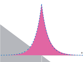
Figure 1: The stationary quasibound state waveform for a force that is 10% of the critical value (the energy of this quasibound state is $E=-1.0955\,E_{b}$). The bound state wave (envelope) of the delta well is shown as the dashed curve, and both are displayed against the backdrop of the full potential energy curve, $-Fx-\lambda\delta(x)$.

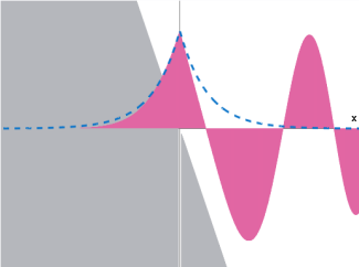
Figure 2: The stationary quasibound state waveform for a force that is 90% of the critical value (the energy of this quasibound state is $E=-0.46404\,E_{b}$). The bound state wave (envelope) of the delta well is shown as the dashed curve, and both are displayed against the backdrop of the full potential energy curve, $-Fx-\lambda\delta(x)$.

Poles in the complex $E$-plane of the continued resolvent operator for $\widehat{H}_{0}+\widehat{V}$ (i.e., resonances) also have been studied for this model potential Moyer2 , Ludviksson -Alvarez . Again, one of these is characterized by a real part that approaches $E_{b}$ as $F\rightarrow 0$ (plus an imaginary part that vanishes exponentially with $F$ in this limit). In fact, the equation for the resonance energies is just Eq.(18) with $Hi(\ldots)$ $=Bi(\ldots)-Gi(\ldots)$ replaced by the (complex-valued) combination $Bi(\ldots)+iAi(\ldots)$. As $F\rightarrow 0$ with $E<0$, the Airy function arguments tend to infinity, where $Bi(\ldots)$ dominates over both $Ai(\ldots)$ and $Gi(\ldots)$ to all orders in the force parameter $F$. It follows that the resonance associated with the bound state of the delta well and the stationary quasibound state with $E<0$ cannot be distinguished in the perturbative regime. This feature actually transcends the example that illustrates it: Ref.Moyer implies that the resonance wave Green’s function differs from Eq.(17) only by terms that are asymptotically small compared to any power of $F$, thus assuring identical perturbation series for any ‘sourcing’ potential $V(x)$. Indeed, the larger point here is one that underscores the central tenet of our theory: Stationary quasibound states and resonances are but different manifestations of those states broadly termed ‘quasibound’, that derive from true bound states by the growth of a parameter. The uniqueness of the Rayleigh–Schrödinger perturbation series ensures that both yield identical expansions in that parameter whenever such developments exist.

VII Application Class: The Spherical Wave Continuum

In this case, the ‘bare’ Hamiltonian $\widehat{H}_{0}$ is the operator for kinetic energy in a three-dimensional space. The spectrum of $\widehat{H}_{0}\$is semi-infinite (bounded from below by $E=0$, but no upper limit) and composed of degenerate levels. There is some flexibility in labeling here depending upon what dynamical variables we opt to conserve along with particle energy. In the angular momentum representation, the stationary states are indexed by a continuous wave number $k$ (any non-negative value), an orbital quantum number $l$ (a non-negative integer), and a magnetic quantum number $m_{l}$ (an integer between $-l$ and $+l$, not to be confused with particle mass): $|\,E\,\rangle\rightarrow|\,klm_{l}\,\rangle$. This stationary state has energy $E_{k}=k^{2}/2m$, and all levels are degenerate with respect to the angular momentum labels $l$ and $m_{l}$. This application class illustrates the role of degeneracy in fixing quasibound states when the interaction $\widehat{V}$ does not mix degenerate states in the continuum.

The eigenfunctions of $\widehat{H}_{0}$ (the spherical waves) are $\langle\,\overrightarrow{r}\,|\,klm_{l}\,\rangle\propto$ $\,j_{l}(kr)Y_{l}^{m_{l}}(\Omega)$ (product of a spherical Bessel function $j_{l}$ with a spherical harmonic $Y_{l}^{m_{l}}$). The degeneracy in the spectrum of $\widehat{H}_{0}$ breeds multiple timelines, and these are conveniently indexed by the same orbital and magnetic quantum numbers that label the spectral states. In the coordinate basis,

$$\langle\,\overrightarrow{r}\,|\,\tau\,\rangle\rightarrow\langle\,\overrightarrow{r}\,|\,\tau lm_{l}\,\rangle=\frac{1}{\sqrt{2\pi}}{\displaystyle\int\limits_{0}^{\infty}}\exp\left(-iE_{k}\tau\right)\,\langle\,\overrightarrow{r}\,|\,klm_{l}\,\rangle\,dE_{k}$$ (20)

We write the time states in the coordinate basis as $\langle\,\overrightarrow{r}\,|\,\tau lm_{l}\,\rangle\equiv\Xi_{\tau}^{l}(r)Y_{l}^{m_{l}}(\Omega)$ where $\Xi_{\tau}^{l}(r)$, the radial piece of the timeline wave, is given by Moyer4

$$\Xi_{\tau}^{l}(r)=\sqrt{\frac{4r}{m}}z^{3/2}\exp\left(ir^{2}z-i\pi\frac{2\alpha+1}{4}\right)\,\left[J_{\alpha+1}\left(r^{2}z\right)-iJ_{\alpha}\left(r^{2}z\right)\right]\text{\qquad}z\equiv\frac{m}{4\tau}$$ (21)

Here $J_{\alpha}$ denotes the [cylinder] Bessel function of order $\alpha$, and $2\alpha\equiv l-1/2$. Eq.(21) is valid for any real $\tau>0$; to obtain results for $\tau<0$, we use

$$\Xi_{-\tau}^{l}(r)=\left[\Xi_{\tau}^{l}(r)\right]^{\ast},$$ (22)

a relation suggested by Eq.(20) and established rigorously in Ref.Moyer4 .

To further explore the properties of $\Xi_{\tau}^{l}(r)$, it is convenient to introduce new functions $h_{\alpha}^{\pm}$, related to Hankel functions of the first and second kind $H_{\alpha}^{(1,2)}$ as

$$h_{\alpha}^{\pm}(z)\equiv\sqrt{\frac{\pi z}{2}}\exp\left(\mp iz\pm i\pi\frac{2\alpha+1}{4}\right)\left[H_{\alpha+1}^{(1,2)}(z)-iH_{\alpha}^{(1,2)}(z)\right]$$ (23)

To be clear, $h_{\alpha}^{+}$ involves only Hankel functions of the first kind, $H^{(1)}$, and $h_{\alpha}^{-}$ only Hankel functions of the second kind, $H^{(2)}$. Like the Hankel functions, $h_{\alpha}^{\pm}(z)$ are regular functions of $z$ throughout the $z$-plane cut along the negative real axis. Using these definitions along with $2J_{\alpha}(z)=H_{\alpha}^{(1)}(z)+H_{\alpha}^{(2)}(z)$ allows us to write Eq.(21) as

$$\Xi_{\tau}^{l}(r)=\sqrt{\frac{2}{\pi mr}}\left[z\exp\left(i2r^{2}z-i\pi\frac{2\alpha+1}{2}\right)h_{\alpha}^{+}(r^{2}z)+zh_{\alpha}^{-}(r^{2}z)\right]\text{\qquad}z\equiv\frac{m}{4\tau},$$ (24)

with $2\alpha\equiv l-1/2$ as before. The virtue of this representation is that $h_{\alpha}^{\pm}(\ldots)$ typically are bounded functions with bounded variation over the entire range of their argument. From their definition, we find that $h_{\alpha}^{\pm}(z)\sim z^{\alpha+1/2}$ for small $\left|z\right|$ and thus bounded as $z\rightarrow 0$ provided $\alpha\geq-1/2$. When $\left|z\right|$ is large, we employ Hankel’s asymptotic series Abramowitz2 for the Hankel functions in Eq.(23), in this way obtaining for any $\alpha>-1/2$ and $\left|\arg(z)\right|<\pi$:

$$h_{\alpha}^{+}(z) =-2i+\frac{\alpha\left(\alpha+1\right)+1/4}{z}+o\left(\frac{1}{z}\right)$$

$$h_{\alpha}^{-}(z) =\frac{\alpha+1/2}{z}+o\left(\frac{1}{z}\right)$$ (25)

In particular, $h_{\alpha}^{+}(z)$ saturates as $\left|z\right|\rightarrow\infty$ and $h_{\alpha}^{-}(z)$ vanishes in this limit.

VII.1 Stationary Quasibound States in the Spherical Wave Continuum

We will assume that the interaction potential has spherical symmetry, $V(\overrightarrow{r})=V(r)$, so that $l$ and $m_{l}$ remain good quantum numbers for the eigenstates of $\widehat{H}=\widehat{H}_{0}+\widehat{V}$. Then the stationary states in the presence of the interaction are $\langle\,\overrightarrow{r}\,|\,\psi_{E}\,\rangle=R_{El}(r)Y_{l}^{m_{l}}(\Omega)$, and the quasibound selection rule for this class reduces to

$${\displaystyle\int\limits_{0}^{\infty}}\,dr\,r^{2}\,\Xi_{\tau}^{l}(r)R_{El}^{\ast}(r)=0$$ (26)

The limiting forms for $\Xi_{\tau}^{l}(r)$, together with the well-known properties of the radial wave $R_{El}(r)$ ($R_{El}(r)\sim r^{l}$ as $r\rightarrow 0$ and $rR_{El}(r)$ bounded as $r\rightarrow\infty$ Merzbacher ) ensure that the integral exists. Moreover, the [effectively non-degenerate] nature of the spectrum again guarantees that $R_{El}(r)$ is real, apart from an overall scale factor. We conclude that the quasibound selection rule is well-formed, and admits real roots $E$ only if $\Xi_{\tau}^{l}(r)$ also is real (apart from a scale factor). Inspection of Eq.(21) shows that $\Xi_{\tau}^{l}(r)$ is complex-valued for any non-zero $\tau$, but also that $\tau=0$ is a singular point for these functions. Thus we are left to examine Eq.(26) in the limit as $\tau\rightarrow 0$ in the hope of recovering a viable rule for distinguishing stationary quasibound states in this application.

To that end, we note that the coefficient of $h_{\alpha}^{+}(\ldots)$ in Eq.(24) is a rapidly varying function of $r$ for $\tau$ small; when substituted into Eq.(26) we get (after changing variables to $u=mr^{2}/2$) a term proportional to

$$\frac{1}{\tau}{\displaystyle\int\limits_{0}^{\infty}}\,du\,u^{\frac{1}{4}}\exp\left(iu/\tau\right)h_{\alpha}^{+}(u/2\tau)R_{El}(r(u))$$

Since $h_{\alpha}^{+}$ is bounded for all values of its argument, this last form is in essence a Fourier integral, whose asymptotics have been thoroughly studied Erdelyi . Assuming that $f(u)\equiv R_{El}(r(u))$ and its derivatives all exist on $0\leq u<\infty$ and vanish as $u\rightarrow\infty$, repeated integration by parts generates an asymptotic series in successive powers of $\tau$. The difficulty here – if there is one – comes at the lower limit ($u=0$), where the inverse transformation $r(u)$ is singular and derivatives of $f(u)$ may be infinite. To circumvent this problem, we assume the power series expansion of $R_{El}(r)$ about $r=0$ includes only even, non-negative powers of $r$, and designate $R_{El}(r)$ as $R_{El}^{+}(r)$ to emphasize this assumption. To exhibit the leading term in the resulting asymptotic series for $\tau$, we integrate by parts once using

$$v_{\tau}(u)\equiv-{\displaystyle\int\limits_{u}^{i\infty}}dt\,t^{\frac{1}{4}}\exp\left(it/\tau\right)h_{\alpha}^{+}(t/2\tau)$$

The path of integration for $v_{\tau}(u)$ lies entirely in the quadrant $0\leq\arg(t)\leq\pi/2$, so the integral above converges absolutely. Then

$$\frac{1}{\tau}{\displaystyle\int\limits_{0}^{\infty}}\,du\,u^{\frac{1}{4}}\exp\left(iu/\tau\right)h_{\alpha}^{+}(u/2\tau)R_{El}^{+}(r(u)) \sim-\frac{1}{\tau}R_{El}^{+}(0)v_{\tau}(0)$$

$$=2R_{El}^{+}(0)\left(2\tau\right)^{\frac{1}{4}}{\displaystyle\int\limits_{0}^{i\infty}}dz\,z^{\frac{1}{4}}\exp\left(i2z\right)h_{\alpha}^{+}(z)$$

This term is at least $O(\tau^{1/4})$ (if $R_{El}^{+}(0)\neq 0$) and therefore vanishes in the limit $\tau\rightarrow 0$.

The preceding argument leaves open the question of how to handle any odd powers in the series expansion of $R_{El}(r)$ about $r=0$. But all odd powers can be grouped together as $rR_{El}^{+}(r)$, where $R_{El}^{+}(r)$ includes only even powers of $r$ as before. The prefactor $r$ translates into an extra factor of $u^{1/2}$, which is absorbed by redefining $v_{\tau}(u)$ as

$$v_{\tau}(u)\equiv-{\displaystyle\int\limits_{u}^{i\infty}}dt\,t^{\frac{3}{4}}\exp\left(it/\tau\right)h_{\alpha}^{+}(t/2\tau)$$

Then repeated integration by parts again produces an asymptotic series in $\tau$, now with a leading term at least $O(\tau^{3/4})$. Thus, the main conclusion reached previously remains intact: such terms make no contribution to the left side of Eq.(26) as $\tau\rightarrow 0$.

By contrast, the term involving $h_{\alpha}^{-}(\ldots)$ makes a contribution to Eq.(26) that is proportional to

$${\displaystyle\int\limits_{0}^{\infty}}\,\frac{dr}{\sqrt{r}}\,\,R_{El}(r)r^{2}zh_{\alpha}^{-}(r^{2}z)$$

Since $r^{2}zh_{\alpha}^{-}(r^{2}z)$ is bounded for all $z$, this integral converges absolutely and uniformly in $\tau$, so the limit $\tau\rightarrow 0$ ($z\rightarrow\infty$) may be taken inside the integral to yield the desired [gauge-invariant] selection rule for stationary quasibound states belonging to this application class:

$${\displaystyle\int\limits_{0}^{\infty}}\,\frac{dr}{\sqrt{r}}\,R_{El}(r)=0$$ (27)

A heuristic argument leading to Eq.(27) also can be given, based on Eq.(13). Using

$$\langle\,klm_{l}\,|\,\psi_{E}\,\rangle\propto{\displaystyle\int\limits_{0}^{\infty}}\,\sqrt{k}j_{l}(kr)R_{El}(r)\,r^{2}dr$$

we substitute into Eq.(13) with $\tau=0$ to get

$${\displaystyle\int\limits_{0}^{\infty}}\,\left[{\displaystyle\int\limits_{0}^{\infty}}\sqrt{k}j_{l}(kr)\,dE_{k}\right]R_{El}(r)\,r^{2}dr=0$$

But

$${\displaystyle\int\limits_{0}^{\infty}}\sqrt{k}j_{l}(kr)\,dE_{k}\propto{\displaystyle\int\limits_{0}^{\infty}}j_{l}(kr)k\sqrt{k}\,dk=\frac{1}{r^{2}\sqrt{r}}{\displaystyle\int\limits_{0}^{\infty}}j_{l}(u)u^{3/2}\,du$$

so Eq.(27) is recovered if the integral on the far right simply exists. Unfortunately $j_{l}$ does not vanish fast enough at infinity to secure convergence, thus necessitating the more elaborate argument given previously.

VII.2 Green’s Function for Stationary Quasibound Spherical Waves

The Green’s function for this class, $G_{E}^{l}(r,r^{\prime})$, is the solution to the radial wave equation with a delta function inhomogeneity:

$$-\frac{1}{2mr^{2}}\frac{\partial}{\partial r}\left(r^{2}\frac{\partial G_{E}^{l}}{\partial r}\right)+\frac{l\left(l+1\right)\hbar^{2}}{2mr^{2}}G_{E}^{l}(r,r^{\prime})-EG_{E}^{l}(r,r^{\prime})=-\frac{\delta(r-r^{\prime})}{r^{2}}$$

For $r\neq r^{\prime}$ the solutions are spherical Bessel functions $j_{l}(kr)$, $y_{l}(kr)$, with $k$ related to the particle energy as $E=k^{2}/2m$. Considered as a function of its first argument, $G_{E}^{l}(r,r^{\prime})$ must be regular at the origin, continuous everywhere, but with a slope discontinuity at $r=r^{\prime}$ as prescribed by the delta-function singularity there. The solution consistent with these constraints can be written compactly as

$$G_{E}^{l}(r,r^{\prime})=\alpha_{l}(r^{\prime})j_{l}(kr)-2mk\,\theta(r-r^{\prime})\left[j_{l}(kr)y_{l}(kr^{\prime})-y_{l}(kr)j_{l}(kr^{\prime})\right]$$ (28)

where $\theta(\ldots)$ is the Heaviside step function and $\alpha_{l}(r^{\prime})$ denotes an as-yet unspecified function. To find $\alpha_{l}(r^{\prime})$ we impose the selection rule, Eq.(27); expressed in the language of the Green’s function, this is

$${\displaystyle\int\limits_{0}^{\infty}}\,\frac{dr}{\sqrt{r}}\,\,G_{E}^{l}(r,r^{\prime})=0\quad\forall r^{\prime}$$

From this we obtain the one additional relation that specifies $\alpha_{l}(r^{\prime})$

$$\alpha_{l}(r^{\prime}){\displaystyle\int\limits_{0}^{\infty}}\,\frac{du}{\sqrt{u}}\,\,j_{l}(u)=2mk{\displaystyle\int\limits_{kr^{\prime}}^{\infty}}\,\frac{du}{\sqrt{u}}\,\,\left[j_{l}(u)y_{l}(kr^{\prime})-y_{l}(u)j_{l}(kr^{\prime})\right]$$ (29)

and with it, the complete Green’s function for stationary quasibound states in the spherical wave application class.

In practice, use of the Green’s function formulation will require a closed form for $\alpha_{l}(r^{\prime})$, a task we leave to future investigation. But the special case of $s$-waves ($l=0$) is sufficiently important and simple enough to address here. Substituting the spherical Bessel functions of index zero, and integrating once by parts gives

$$kr^{\prime}{\displaystyle\int\limits_{kr^{\prime}}^{\infty}}\,\frac{du}{\sqrt{u}}\,\left[j_{0}(u)y_{0}(kr^{\prime})\,-\,y_{0}(u)j_{0}(kr^{\prime})\right] =-2{\displaystyle\int\limits_{kr^{\prime}}^{\infty}}\,\frac{du}{\sqrt{u}}\cos\left(kr^{\prime}-u\right)$$

$$=-2\sqrt{2\pi}\,g\left(\sqrt{\frac{2kr^{\prime}}{\pi}}\right)$$ (30)

Here $g(\ldots)$ is the Fresnel auxiliary function Abramowitz4 , a non-negative, monotonically decreasing function on $[0,\infty)$ with limit values $g(0)=1/2$ and $g(\infty)=0$. Also, we can let $kr^{\prime}\rightarrow 0$ in Eq.(30) to recover the special value

$${\displaystyle\int\limits_{0}^{\infty}}\,\frac{du}{\sqrt{u}}\,\,j_{0}(u)=2\sqrt{2\pi}g(0)=\sqrt{2\pi}$$

Putting it all together, we obtain the Green’s function for stationary quasibound $s$-waves ($l=0$) in the form

$$G_{E}^{0}(r,r^{\prime})=-\frac{2m}{r^{\prime}}2g\left(\sqrt{\frac{2kr^{\prime}}{\pi}}\right)\frac{\sin(kr)}{kr}+\frac{2m}{r^{\prime}}\,\theta(r-r^{\prime})\frac{\sin(kr-kr^{\prime})}{kr}$$ (31)

VII.3 Example: $s$-States in a Leaky Spherical Well

To illustrate quasibound states in the present context, we take for $V(r)$ a spherically-symmetric barrier of height $V_{0}>0$ extending from $r=a$ to $r=b$, and zero elsewhere. Such a barrier effectively creates a ‘leaky’ spherical well of radius $a$ centered at the coordinate origin. There are no true bound states for this potential, except in the limit of zero barrier transparency ($b\rightarrow\infty$ and/or $V_{0}\rightarrow\infty$).

Radial wave functions for the $s$-wave ($l=0$) quasibound states introduced by $V$ satisfy

$$R_{E}(r)={\displaystyle\int\limits_{0}^{\infty}}\,dr^{\prime}\,r^{\prime 2}G_{E}^{0}(r,r^{\prime})V(r^{\prime})R_{E}(r^{\prime})$$

For $s$-waves, we prefer a formulation in terms of the effective one-dimensional wave function $u_{E}(r)\equiv rR_{E}(r)$; for the leaky spherical well, this becomes

$$u_{E}(r) =V_{0}{\displaystyle\int\limits_{a}^{b}}\,dr^{\prime}r\,r^{\prime}G_{E}^{0}(r,r^{\prime})u_{E}(r^{\prime})$$

$$=-\frac{2mV_{0}}{k}\sin(kr){\displaystyle\int\limits_{a}^{b}}\,dr^{\prime}2g\left(z(r^{\prime})\right)u_{E}(r^{\prime})+\frac{2mV_{0}}{k}{\displaystyle\int\limits_{a}^{b}}\,dr^{\prime}\theta(r-r^{\prime})\sin(kr-kr^{\prime})u_{E}(r^{\prime})$$

where for brevity we have introduced $z(r)\equiv\sqrt{2kr/\pi}$. We see immediately that $u_{E}(r)\propto\sin(kr)$ for $r\leq a$, as expected. For $a\leq r\leq b$ and $V_{0}>E$, $u_{E}(r)$ should be a combination of growing and decaying exponentials $\exp\left(\pm\kappa r\right)$ with $\kappa^{2}=2m\left(V_{0}-E\right)$. If, in the barrier region, we write

$$u_{E}(r)=\exp(-\kappa r)+s\exp(\kappa r)\qquad a\leq r\leq b$$

then continuity of the logarithmic derivative of $u_{E}(r)$ at $r=a$ specifies the mixing coefficient $s$ as

$$s=\exp(-2\kappa a)\frac{\kappa\sin(ka)+k\cos(ka)}{\kappa\sin(ka)-k\cos(ka)}$$ (32)

Enforcing continuity of $u_{E}(r)$ at $r=a$ then leads to

$$\exp(-\kappa a)+s\exp(\kappa a)=-\frac{2mV_{0}}{k}\sin(ka){\displaystyle\int\limits_{a}^{b}}\,dr\,2g\left(z(r)\right)\left[\exp(-\kappa r)+s\exp(\kappa r)\right]$$

Finally, substituting for $s$ from Eq.(32) and rearranging gives

$$-1 =\left[\frac{\kappa}{k}\sin(ka)-\cos(ka)\right]\,\frac{2mV_{0}}{\kappa}{\displaystyle\int\limits_{a}^{b}}\,dr\,g\left(z(r)\right)\exp(\kappa a-\kappa r)$$

$$+\left[\frac{\kappa}{k}\sin(ka)+\cos(ka)\right]\,\frac{2mV_{0}}{\kappa}{\displaystyle\int\limits_{a}^{b}}\,dr\,g\left(z(r)\right)\exp(\kappa r-\kappa a)$$ (33)

Despite appearances, $k$ and $\kappa$ are not independent here, but linked for a given potential barrier by the familiar relation

$$k^{2}+\kappa^{2}=2mV_{0}$$

Eq.(33) as written is valid for $E<V_{0}$; it is an implicit equation whose roots $ka$ prescribe the stationary quasibound states with below-the-barrier energy in this leaky well. Roots must be found numerically, but several noteworthy observations can be made without further computation:

1. In the thick barrier limit ($b\rightarrow\infty$) the last integral on the right of Eq.(33) diverges, whereas the remaining terms are bounded for all $k,\kappa>0$. It follows that the coefficient of the divergent integral must vanish in this limit. Eq.(33) further suggests that this coefficient approaches zero exponentially in $b$. Indeed, careful analysis shows that for large $b$ ($w\equiv b-a$ is the barrier width)

   $$\frac{\kappa}{k}\sin(ka)+\cos(ka)\sim b^{3/2}\exp\left(-\kappa w\right)$$

   Since the zeros of the expression on the left specify the bound state energies of a spherical well with width $a$, we conclude that the stationary quasibound levels merge with those bound state levels as $b\rightarrow\infty$. Also since there is no degeneracy in the $s$-wave spectrum – either with or without the ‘sourcing’ potential $V(r)$ – it follows that the stationary quasibound waveforms themselves converge to the bound state wave functions of the spherical well in this limit.

2. As the barrier narrows, the right side of Eq.(33) steadily shrinks in magnitude until that equation is incapable of supporting solutions. To explore this point further, we rewite Eq.(33) in the abbreviated form

   $$-1=A\frac{\sin(ka)}{ka}+B\cos(ka)$$

   with obvious definitions for $A$ and $B$. Since $g\left(z\right)$ is a monotonically decreasing function, we easily deduce the bounds

   $$A \lesssim 2mV_{0}aw\frac{\sinh\left(\kappa w\right)}{\left(\kappa w\right)}2g\left(z_{a}\right)=2mV_{0}aw\frac{\sinh\left(\kappa w/2\right)\cosh\left(\kappa w/2\right)}{\left(\kappa w/2\right)}2g\left(z_{a}\right)$$

   $$B \lesssim 2mV_{0}w^{2}\frac{\cosh\left(\kappa w\right)-1}{\left(\kappa w\right)^{2}}2g\left(z_{a}\right)=2mV_{0}w^{2}\left[\frac{\sinh\left(\kappa w/2\right)}{\left(\kappa w/2\right)}\right]^{2}g\left(z_{a}\right)$$ (34)

   For a thin barrier ($\tanh\left(\kappa w/2\right)\ll\kappa a/2$), $A$ appears to be dominant and the equation for the quasibound energies becomes, approximately,

   $$-1\simeq 2mV_{0}aw\frac{\sinh\left(\kappa w\right)}{\left(\kappa w\right)}\left[2g\left(\sqrt{\frac{2ka}{\pi}}\right)\frac{\sin(ka)}{ka}\right]$$

   Considered as a function of $ka$, the bracketed term on the right is a steadily decaying oscillation about zero. Numerical investigation shows that the first (deepest) minimum occurs at $ka\simeq 4.2149$, and the function value at this point is $\approx-1/120$. It follows that no stationary quasibound states can exist if

   $$2mV_{0}aw\frac{\sinh\left(\kappa w\right)}{\left(\kappa w\right)}\leq\sqrt{2mV_{0}a^{2}}\sinh\left(\sqrt{2mV_{0}w^{2}}\right)\lesssim 120$$ (35)

   Although not rigorous, the bound of Eq.(35) is sufficiently accurate as to be quite useful in practice.

The integrals appearing in Eq.(33) can actually be done in closed form with the help of the following [indefinite] integral:

$$\left[1+\frac{\pi^{2}}{4\gamma^{2}}\right]{\displaystyle\int^{z}}\,d(\gamma z^{2})\,g\left(z\right)\exp(\gamma z^{2})=\left[g\left(z\right)-\frac{\pi}{2\gamma}f(z)\right]\exp(\gamma z^{2})+i\sqrt{\frac{\pi}{4\gamma}}\operatorname{erf}\left(-i\sqrt{\gamma}\,z\right)$$ (36)

Here $f(z)$ is the Fresnel auxiliary function companion to $g(z)$ Abramowitz4 , and $\operatorname{erf}\left(\ldots\right)$ denotes the familiar error function. This result allows direct numerical computation of the stationary quasibound levels for this example. A thorough analysis is out of place here, but may appear in a future publication.

Resonances for twin symmetric barriers have been investigated by Maheswari, et. al. Maheswari . The antisymmetric states in their study become the $s$-wave resonances for the leaky well described here. They report numerical results for the lowest 8-10 resonance energies (along with their widths) generated by a relatively thin ($w=0.167\,a$), as well as a moderately thick ($w=0.5\,a$) rectangular barrier, with $V_{0}a^{2}=72$ (in units where $\hbar^{2}=2m=1$) for both. Only the latter is thick enough to support any stationary quasibound states. [With $V_{0}a^{2}=72$, the critical barrier thickness implied by Eq.(35) is $w_{cr}\simeq 0.394\,a$, whereas the actual value $w_{cr}\simeq 0.425\,a$ is about $7\%$ larger.] Our calculations show that for $V_{0}a^{2}=72$ and $w=0.5\,a$ the lowest-lying stationary quasibound state has energy $E=1.067$. And there is just one additional stationary quasibound state for these parameter values, at energy $E=2.331$. For comparison, Maheswari, et. al. find – using these same parameters – three antisymmetric resonances below the top of the barrier ($E_{r}<V_{0}$), at energies $E_{r}=0.874$, $3.444$, and $7.421$.

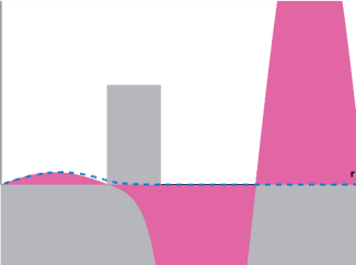
Figure 3: The lowest-lying quasibound $s$-state for a spherically-symmetric barrier, with $V_{0}a^{2}=72$ and $w=0.5\,a$. The bound state wave (envelope) of the spherical well that results from an infinitely thick barrier is shown as the dashed curve, and both are displayed against the backdrop of the barrier potential $V(r)$.

The differences between stationary quasibound states and resonances are evident in these results, perhaps in no small part because a perturbative treatment is not possible here, and because with the chosen parameters even the most stable of the stationary quasibound states is on the verge of extinction. The wave function for the lowest-lying stationary quasibound state is shown in Fig. 3, where it is compared with the bound state wave to which it converges in the thick barrier limit $b\rightarrow\infty$. The resemblance is clear inside the spherical well ($0\leq r\leq a$) and just beyond, but there the similarities end. The bound state wave continues to decay exponentially with $r$, while the quasibound waveform emerges at the outer barrier edge with considerable amplitude and is oscillatory beyond. [The external wave amplitude actually grows with increasing $b$, even as the waveform up to and including the first node converges smoothly to the bound state wave.] With these same parameters, the associated resonance has energy (real part) indistinguishable from that of the bound state ($E_{r}=0.874$) to the accuracy reported, making the resonance and bound state wave functions virtually identical over the range shown. Still, the imaginary part of the resonance energy – though quite small ($E_{i}=-\,0.718\times 10^{-4}$) – causes the resonance wave to diverge exponentially in the asymptotic region $r\rightarrow\infty$.

VIII Application Class: The Free Particle Continuum in One Dimension

For this case $\widehat{H}_{0}$ describes a particle free to move along the line $-\infty<x<\infty$. The eigenfunctions of $\widehat{H}_{0\text{ }}$are harmonic waves with wavenumber $k$ and energy $E_{k}=k^{2}/2m$. Since $k$ can be any real number, the spectrum extends from $E_{k}=0$ to $E_{k}=\infty$ and each energy level is doubly-degenerate ($\pm k$). This application class illustrates how spectral degeneracy affects the search for stationary quasibound states when the interaction giving rise to those states actually mixes degenerate states in the continuum.

The eigenfunctions may be taken as plane waves, and plane waves running in opposite directions give rise to distinct quantum histories. Alternatively, histories can be constructed from standing wave combinations of these plane waves, and is the course we follow here. Timeline elements in the standing wave picture are described by the coordinate-space forms $\langle\,x\,|\,\tau\pm\rangle\equiv\Xi_{\tau}^{\pm}(x)$ where the sign label $\left(\pm\right)$ specifies the parity of these waves.

The odd-parity states are simply related to the timeline states for spherical waves with $l=0$; indeed, $\sqrt{2}\,\Xi_{\tau}^{-}(x)=x\,\Xi_{\tau}^{0}(x)$ Moyer4 . Applying the result of Eq.(24) to this case ($\alpha=-1/4$), we obtain for $x\geq 0$ and $\tau>0$

$$\Xi_{\tau}^{-}(x)=\sqrt{\frac{x}{\pi m}}\left[z\exp\left(i2x^{2}z-i\pi/4\right)h_{-1/4}^{+}(x^{2}z)+zh_{-1/4}^{-}(x^{2}z)\right]\text{\qquad}z\equiv\frac{m}{4\tau}$$ (37)

It is noteworthy that the odd-parity states by themselves constitute a complete history for an otherwise free particle that is confined to the half-axis $x>0$ (by an infinite potential wall at the origin). But for a truly free particle we also need the even-parity states.

For the even-parity states, we exploit the formal connection to time states for spherical waves with $l=-1$: $\sqrt{2}\,\Xi_{\tau}^{+}(x)=x\,\Xi_{\tau}^{-1}(x)$ Moyer4 . While unphysical for spherical waves, Eq.(24) continues to hold for $l=-1$ ($\alpha=-3/4$) and gives for $x\geq 0$ and $\tau>0$

$$\Xi_{\tau}^{+}(x)=\sqrt{\frac{x}{\pi m}}\left[z\exp\left(i2x^{2}z+i\pi/4\right)h_{-3/4}^{+}(x^{2}z)+zh_{-3/4}^{-}(x^{2}z)\right]\text{\qquad}z\equiv\frac{m}{4\tau}$$ (38)

The extension of these results to $\tau<0$ is afforded by Eq.(22); the extension to $x<0$ is dictated by parity.

VIII.1 Stationary Quasibound States in the Free-Particle Continuum

In the present context, there are a pair of enforceable conditions leading to two distinct kinds of quasibound states: they are

$${\displaystyle\int\limits_{-\infty}^{\infty}}\,dx\,\,\Xi_{\tau}^{\pm}(x)\psi_{E}^{\ast}(x)=0$$ (39)

where again $\psi_{E}(x)\equiv\langle\,x\,|\,\psi_{E}\,\rangle$ is the Schrödinger waveform for the stationary state of $\widehat{H}_{0}+\widehat{V}$ with energy $E$. So long as $\psi_{E}(x)$ is everywhere bounded, the integrals of Eq.(39) exist and the quasibound state criteria are well-formed. While $\psi_{E}(x)$ is not guaranteed to be real, its complex conjugate is a stationary state wave with the same energy. Thus, we may form two new states $\psi_{E}(x)\pm\psi_{E}^{\ast}(x)$ which are real up to a constant multiplier. In effect, without loss of generality we can always assume $\psi_{E}(x)$ is real (apart from a constant multiplier) in Eq.(39) for the purpose of computing quasibound states. Furthermore, the candidate wave function can always be split into even and odd parts, $\psi_{E}(x)=\psi_{E}^{+}(x)+\psi_{E}^{-}(x)$, such that

$$\psi_{E}^{\pm}(x)=\frac{1}{2}\left[\psi_{E}(x)\pm\psi_{E}(-x)\right]$$

are themselves real (again apart from a constant multiplier). With this decomposition, the quasibound criteria of Eq.(39) reduce to

$${\displaystyle\int\limits_{0}^{\infty}}\,dx\,\,\Xi_{\tau}^{\pm}(x)\psi_{E}^{\pm}(x)=0$$ (40)

where either the upper or lower signs are taken together. The odd-parity case ($-$) is formally identical to that for spherical $s$-waves with the replacement $R_{El}(r)\rightarrow$ $x^{-1}\psi_{E}^{-}(x)$; thus for $u=mx^{2}/2$, so long as $f(u)\equiv\left[x(u)\right]^{-1}\psi_{E}^{-}(x(u))$ and its derivatives all exist on $0\leq u<\infty$ and vanish as $u\rightarrow\infty$, we are led in the same way to one [gauge-invariant] selection rule for stationary quasibound states belonging to this application class:

$${\displaystyle\int\limits_{0}^{\infty}}\,\frac{dx}{\sqrt[3]{x}}\,\psi_{E}^{-}(x)=0$$ (41)

The even-parity case is a bit trickier. Let us define

$$I_{\tau}(x)\equiv{\displaystyle\int\limits_{0}^{x}}\Xi_{\tau}^{+}(x^{\prime})\,dx^{\prime}$$

Using the properties of Bessel functions, it is a straightforward exercise to show that this integral can be evaluated in terms of $\Xi_{\tau}^{+}(x)$ and the time state for $p$-waves, $\Xi_{\tau}^{1}(x)$:

$$I_{\tau}(x)=x\Xi_{\tau}^{+}(x)+\frac{x^{2}}{\sqrt{2}}\Xi_{\tau}^{1}(x)$$

Then from Eq.(38) and the spherical wave result of Eq.(24) with $l=1$ ($\alpha=1/4$), we obtain a corresponding expression for $I_{\tau}(x)$:

$$I_{\tau}(x)=\sqrt{\frac{x^{3}}{\pi m}}\left[\exp\left(i2x^{2}z+i\pi/4\right)z\left(h_{-3/4}^{+}(x^{2}z)-h_{1/4}^{+}(x^{2}z)\right)+zh_{-3/4}^{-}(x^{2}z)+zh_{1/4}^{-}(x^{2}z)\right]$$ (42)

The asymptotic results for $h^{\pm}$ from Eq.(25) show that $I_{\tau}(x)$ vanishes as $x\rightarrow\infty$; thus, Eq.(40) can be integrated once by parts to express the quasibound state criterion for the even-parity case in the alternate form

$${\displaystyle\int\limits_{0}^{\infty}}\,dx\,I_{\tau}(x)\frac{d\psi_{E}^{+}}{dx}=0$$ (43)

From this point on, the argument parallels that given previously for the case of spherical waves. Real energy solutions to Eq.(43) demand that $I_{\tau}(x)$ be real and this, in turn, requires $\tau\rightarrow 0$. The coefficient of $h_{\alpha}^{+}(\ldots)$ ($\alpha=-3/4,\,1/4$) in Eq.(42) is a rapidly-varying function of $x$ for $\tau$ small; when substituted into Eq.(43) these generate terms proportional to (after changing variables to $u=mx^{2}/2$)

$$\frac{1}{\tau}{\displaystyle\int\limits_{0}^{\infty}}\,du\,u^{\frac{3}{4}}\exp\left(iu/\tau\right)h_{\alpha}^{+}(u/2\tau)\left[\frac{1}{x}\frac{d\psi_{E}^{+}}{dx}\right]$$

So long as $f(u)\equiv\left[x(u)\right]^{-1}d\psi_{E}^{+}/dx$ and its derivatives all exist on $0\leq u<\infty$ and vanish as $u\rightarrow\infty$, repeated integration by parts generates an asymptotic series in successive powers of $\tau$. To obtain the leading term in that series, we integrate by parts once using

$$v_{\tau}(u)\equiv-{\displaystyle\int\limits_{u}^{i\infty}}dt\,t^{\frac{3}{4}}\exp\left(it/\tau\right)h_{\alpha}^{+}(t/2\tau)$$

with the integration contour confined to the quadrant $0\leq\arg(t)\leq\pi/2$. Then

$$\frac{1}{\tau}{\displaystyle\int\limits_{0}^{\infty}}\,du\,u^{\frac{3}{4}}\exp\left(iu/\tau\right)h_{\alpha}^{+}(u/2\tau)\left[\frac{1}{x}\frac{d\psi_{E}^{+}}{dx}\right] \sim-\frac{1}{\tau}\left[\frac{1}{x}\frac{d\psi_{E}^{+}}{dx}\right]_{0}v_{\tau}(0)$$

$$=\left[\frac{1}{x}\frac{d\psi_{E}^{+}}{dx}\right]_{0}2\left(2\tau\right)^{\frac{3}{4}}{\displaystyle\int\limits_{0}^{i\infty}}dz\,z^{\frac{3}{4}}\exp\left(i2z\right)h_{\alpha}^{+}(z)$$

Evidently such contributions are at least $O\left(\tau^{3/4}\right)$, and therefore vanish in the limit $\tau\rightarrow 0$. By contrast, the remaining terms in Eq.(42) make a contribution proportional to

$${\displaystyle\int\limits_{0}^{\infty}}\,dx\,\sqrt{x^{3}}\,\left[zh_{-3/4}^{-}(x^{2}z)+zh_{1/4}^{-}(x^{2}z)\right]\frac{d\psi_{E}^{+}}{dx}$$

Since $x^{2}zh_{\alpha}^{-}(x^{2}z)$ is bounded for all $z$, this integral converges uniformly in $\tau$ (but not absolutely), so the limit $\tau\rightarrow 0$ ($z\rightarrow\infty$) may be taken inside the integral to yield a second [gauge-invariant] selection rule for stationary quasibound states in this application class:

$${\displaystyle\int\limits_{0}^{\infty}}\,\frac{dx}{\sqrt{x}}\,\,\frac{d\psi_{E}^{+}}{dx}=0$$ (44)

Interestingly, the first selection rule, Eq.(41), can be cast in identical form with the help of a single integration by parts. Thus, both quasibound selection rules for this application class can be expressed by the single compact equation

$${\displaystyle\int\limits_{0}^{\infty}}\,\frac{dx}{\sqrt{x}}\,\,\frac{d\psi_{E}^{\pm}}{dx}=0$$ (45)

where $\psi_{E}^{\pm}(x)$ are the even ($+$) and odd ($-$) parts of the stationary state wave function with energy $E$.

VIII.2 Green’s Function Formulation

The Green’s function $G_{E}(x,x^{\prime})$ for this case is the solution to the free-particle Schrödinger equation with a delta function inhomogeneity. Like the stationary states, $G_{E}(x,x^{\prime})$ can be split into components that are even and odd under reflection (in the first argument); we write this as $G_{E}(x,x^{\prime})=G_{E}^{+}(x,x^{\prime})+G_{E}^{-}(x,x^{\prime})$ where

$$G_{E}^{\pm}(x,x^{\prime})=\frac{1}{2}\left[G_{E}(x,x^{\prime})\pm G_{E}(-x,x^{\prime})\right]$$

clearly has the property $G_{E}^{\pm}(-x,x^{\prime})=\pm G_{E}^{\pm}(x,x^{\prime})$. These component Green’s functions satisfy the differential equation

$$-\frac{1}{2m}\frac{\partial^{2}G_{E}^{\pm}}{\partial x^{2}}-EG_{E}^{\pm}(x,x^{\prime})=-\frac{1}{2}\left[\delta(x-x^{\prime})\pm\delta(x+x^{\prime})\right]$$ (46)

For stationary quasibound states, solutions also must conform to the criteria (cf. Eq.(45))

$${\displaystyle\int\limits_{0}^{\infty}}\,\frac{dx}{\sqrt{x}}\frac{\partial G_{E}^{\pm}(x,x^{\prime})}{\partial x}\,=0\qquad\forall x^{\prime}$$ (47)

Changing the sign of $x^{\prime}$ in Eqs.(46) and (47) implies that $G_{E}^{\pm}(x,-x^{\prime})$ $=\pm G_{E}^{\pm}(x,x^{\prime})$, i.e., the component Green’s functions exhibit the same symmetry under reflection in the second argument as they do for the first argument. It follows that we need only construct $G_{E}^{\pm}(x,x^{\prime})$ over the range $x,x^{\prime}\geq 0$.

Consider first the odd-parity component $G_{E}^{-}(x,x^{\prime})$. For $x,x^{\prime}\geq 0\$this is intimately related to the Green’s function for spherical $s$-waves $G_{E}^{0}(r,r^{\prime})$: indeed, we easily discover that $2G_{E}^{-}(x,x^{\prime})=$ $xx^{\prime}G_{E}^{0}(x,x^{\prime})$. More precisely (cf. Eq.(31)),

$$G_{E}^{-}(x,x^{\prime})=-\frac{m}{k}2g\left(\sqrt{\frac{2kx^{\prime}}{\pi}}\right)\sin(kx)+\frac{m}{k}\,\theta(x-x^{\prime})\sin(kx-kx^{\prime})\qquad x,x^{\prime}\geq 0$$ (48)

For the even-parity component $G_{E}^{+}(x,x^{\prime})$, solutions to Eq.(46) for $x\neq x^{\prime}$ are free-particle standing waves with wavenumber $k$ and energy $E=k^{2}/2m$ that have vanishing slope at $x=0$. For $x,x^{\prime}\geq 0$ we write this as

$$G_{E}^{+}(x,x^{\prime})=\begin{array}[c]{ccc}\alpha(x^{\prime})\cos(kx)&&0\leq x\leq x^{\prime}\\ \beta(x^{\prime})\cos(kx)+\gamma(x^{\prime})\sin(kx)&&x>x^{\prime}\geq 0\end{array}$$

Continuity at $x=x^{\prime}$ requires

$$\left[\alpha(x^{\prime})-\beta(x^{\prime})\right]\cos(kx^{\prime})=\gamma(x^{\prime})\sin(kx^{\prime}),$$

while integrating the differential equation across the singular point at $x=x^{\prime}$ gives

$$\left[\beta(x^{\prime})-\alpha(x^{\prime})\right]\frac{d}{dx^{\prime}}\cos(kx^{\prime})+\gamma(x^{\prime})\frac{d}{dx^{\prime}}\sin(kx^{\prime})=m$$

Combining these matching conditions with the Wronskian $W\left\{\cos z,\sin z\right\}=1$ leads to

$$\gamma(x^{\prime}) =\frac{m}{k}\cos(kx^{\prime})$$

$$\alpha(x^{\prime})-\beta(x^{\prime}) =\frac{m}{k}\sin(kx^{\prime})$$

The specification of $G_{E}^{+}(x,x^{\prime})$ is completed by imposing the selection rule for stationary quasibound states, Eq.(47). After some manipulation, we find for any value of $x^{\prime}\geq 0$

$$\alpha(x^{\prime}){\displaystyle\int\limits_{0}^{\infty}}\,\frac{du}{\sqrt{u}}\sin u=\frac{m}{k}{\displaystyle\int\limits_{kx^{\prime}}^{\infty}}\,\frac{du}{\sqrt{u}}\cos\left(u-kx^{\prime}\right)$$

The integral on the left is related to the Fresnel sine integral $S(\infty)$ and evaluates to $\sqrt{2\pi}$ Abramowitz4 , while the one on the right is essentially the Fresnel auxiliary function $g(\ldots)$ introduced in Sec. VII (cf. Eq.(30)). Collecting all the above results leads to the Green’s function for even-parity stationary quasibound states in the form

$$G_{E}^{+}(x,x^{\prime})=\frac{m}{k}\,2g\left(\sqrt{\frac{2kx^{\prime}}{\pi}}\right)\cos(kx)+\frac{m}{k}\,\theta(x-x^{\prime})\sin(kx-kx^{\prime})\qquad x,x^{\prime}\geq 0$$ (49)

VIII.3 Example: Twin Rectangular Barriers

We consider here a pair of identical rectangular barriers located a distance $a$ to either side of the coordinate origin. The potential energy $V(x)$ is constant at $V_{0}>0$ within the barrier regions $-b\leq x\leq-a$ and $a\leq x\leq b$, and zero elsewhere. The barrier thickness is $w=b-a$. The twin barriers effectively delineate the edges of a ‘leaky’ well of width $2a$ centered at the coordinate origin.

Since $V(x)$ has reflection symmetry about the origin, the stationary states can be taken even or odd under reflection, and only the half-axis $x\geq 0$ need be considered. Stationary quasibound states having odd parity must satisfy the integral equation

$$\psi_{E}^{-}(x)=2{\displaystyle\int\limits_{0}^{\infty}}\,dx^{\prime}\,G_{E}^{-}(x,x^{\prime})V(x^{\prime})\psi_{E}^{-}(x^{\prime})$$

This is the same problem encountered in the previous section for $s$-wave quasibound states in a leaky spherical well of radius $a$, and leads to identical results; accordingly, we will not pursue the odd-parity case any further here.

For the even-parity case, we have simil;arly

$$\psi_{E}^{+}(x) =2{\displaystyle\int\limits_{0}^{\infty}}\,dx^{\prime}\,G_{E}^{+}(x,x^{\prime})V(x^{\prime})\psi_{E}^{+}(x^{\prime})$$

$$=\frac{2mV_{0}}{k}\cos(kx){\displaystyle\int\limits_{a}^{b}}\,dx^{\prime}2g\left(\sqrt{\frac{2kx^{\prime}}{\pi}}\right)\psi_{E}^{+}(x^{\prime})+\frac{2mV_{0}}{k}{\displaystyle\int\limits_{a}^{b}}\,dx^{\prime}\theta(x-x^{\prime})\sin(kx-kx^{\prime})\psi_{E}^{+}(x^{\prime})$$

We see that $\psi_{E}^{+}(x)\propto\cos(kx)$ for $x\leq a$. For $a\leq x\leq b$ (barrier region) and $E<V_{0}$, $\psi_{E}^{+}(x)$ will be a combination of growing and decaying exponentials with decay constant $\kappa$, where $\kappa^{2}=2m\left(V_{0}-E\right)$. Enforcing continuity of the wave and its slope at $x=a$ (the inner barrier edge) leads to the equation specifying the [below-the-barrier] energies of any even-parity, stationary quasibound states in this ‘leaky’ well:

$$1 =\left[\frac{\kappa}{k}\cos(ka)+\sin(ka)\right]\frac{2mV_{0}}{\kappa}{\displaystyle\int\limits_{a}^{b}}\,dx\,g\left(\sqrt{\frac{2kx}{\pi}}\right)\exp(\kappa a-\kappa x)$$

$$+\left[\frac{\kappa}{k}\cos(ka)-\sin(ka)\right]\frac{2mV_{0}}{\kappa}{\displaystyle\int\limits_{a}^{b}}\,dx\,g\left(\sqrt{\frac{2kx}{\pi}}\right)\exp(\kappa x-\kappa a)$$ (50)

The details have been omitted, since they parallel those already given in connection with the example of the ‘leaky’ spherical well discussed in Sec. VII. In fact, Eq.(50) is very similar to Eq.(33), and can be analyzed in much the same way. In particular, we are led to the following observations:

1. In the thick barrier limit ($b\rightarrow\infty$) the last integral on the right of Eq.(50) diverges, whereas the remaining terms are bounded for all $k,\kappa>0$. It follows that the coefficient of the divergent integral must vanish in this limit. Careful analysis of Eq.(50) shows that for large $b$

   $$\frac{\kappa}{k}\cos(ka)-\sin(ka)\sim b^{3/2}\exp\left(-\kappa w\right)$$

   Since the zeros of the expression on the left locate the energies of even-parity states in the finite square well of width $2a$, the even-parity stationary quasibound levels evidently merge with those bound state energies in the limit $b\rightarrow\infty$. Also since there is but one even-parity state at each energy – either with or without the ‘sourcing’ potential $V(x)$ – the stationary quasibound state waveforms must converge to the even-parity bound state wave functions of the finite well in this limit.

2. Unlike the odd-parity case, there is no minimum barrier thickness required to sustain even-parity quasibound states in the central well, so at least one such state always exists. A more refined statement follows by writing Eq.(50) in the form

   $$1=A\frac{\cos(ka)}{ka}-B\sin(ka)$$

   where $A$ and $B$ are the same expressions encountered previously in our study of the ‘leaky’ spherical well, and subject to the estimates Eq.(34). The reasoning employed there indicates that the term involving $A$ is dominant for a narrow barrier, leaving the approximate equation

   $$1\simeq 2mV_{0}aw\frac{\sinh\left(\kappa w\right)}{\left(\kappa w\right)}\left[2g\left(\sqrt{\frac{2ka}{\pi}}\right)\frac{\cos(ka)}{ka}\right]$$

   Considered as a function of $ka$, the bracketed expression clearly diverges as $ka\rightarrow 0$ (thereby guaranteeing at least one root no matter how narrow the barrier), but diminishes rapidly and oscillates about zero with ever-decreasing amplitude as $ka$ grows larger. Numerical investigation shows that the first (highest) maximum is reached for $ka\simeq 5.90$ and the function value there is $\approx 1/248$. We conclude that multiple even-parity, stationary quasibound states are unsustainable if

   $$2mV_{0}aw\frac{\sinh\left(\kappa w\right)}{\left(\kappa w\right)}\leq\sqrt{2mV_{0}a^{2}}\sinh\left(\sqrt{2mV_{0}w^{2}}\right)\lesssim 248$$ (51)

   Again, the bound of Eq.(51) is not rigorous, but represents a reasoned estimate that can guide more in-depth studies.

For resonances in the scattering from twin symmetric barriers, we turn again to the work of Maheswari, et. al. Maheswari , this time with focus on the symmetric states described in their study. With $V_{0}a^{2}=72$ (in units where $\hbar^{2}=2m=1$) and $w=0.5\,a$ they report three symmetric resonances below the top of the barrier ($E_{r}<V_{0}$), at energies $E_{r}=0.219$, $1.955$, and $5.298$. Using the same parameter values, we find just one even-parity, stationary quasibound state at energy $E=0.199$. The wave function for this quasibound state is shown in Fig. 4, where it is compared with the bound state wave function to which it converges in the thick barrier limit $b\rightarrow\infty$. The two are in good agreement where they must be, viz., within the central well and near the inner barrier edge; they differ noticeably in the outer half of the barrier and beyond. Our finding of only one quasibound state is actually inconsistent with the bound of Eq.(51), which for $V_{0}a^{2}=72$ predicts a critical barrier thickness $w_{cr}\simeq 0.480\,a$. In fact, the actual value is about $7\%$ larger, at $w_{cr}\simeq 0.517\,a$. This level of discrepancy is not surprising given the lack of rigor inherent in Eq.(51).

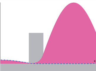
Figure 4: The lowest-lying even-parity quasibound state in the ‘leaky’ well formed by twin barriers, with $V_{0}a^{2}=72$ and $w=0.5\,a$. The bound state wave (envelope) of the well resulting from infinitely thick barriers is shown as the dashed curve, and both are displayed against the backdrop of the twin barrier potential $V(x)$. Only the half-axis $x\geq 0$ is shown.

IX Summary and Conclusions

In this paper we have advocated the viewpoint that states described as ‘quasibound’ should exhibit a connectedness (in the mathematical sense) to true bound states through the growth of some parameter. And we have demonstrated how this connectedness can be formulated in a rigorous way using the novel concept of quantum histories, or timelines, that span the Hilbert space of physical states. The principle that a change of gauge cannot influence the outcome of a measurement restricts the quasibound states to one of two basic types: (1) stationary quasibound states that are characterized by real energies and Schrödinger wave functions that are everywhere bounded (but not square-integrable), and (2), resonant states having complex energies (and consequently divergent waveforms) that correspond to poles in the complex $E$-plane of the scattering or $S$-matrix. Heretofore, only the latter have been recognized in much of the quasibound state literature. That both are rooted in the same underlying principle of connectedness leads to the expectation that stationary quasibound states and resonant states admit identical perturbation expansions in the growth parameter whenever such series developments exist, i.e., the two quasibound types cannot be distinguished in the perturbative regime.

The general theory has been applied to three diverse systems exemplifying distinct spectral characteristics (bounds, degeneracies) of the Hamiltonian for the embedding continuum. Within each such application class, the stationary quasibound states of a model system have been explored and compared with previously reported results for resonant states. The calculations are aimed at highlighting the differences between the two basic quasibound types, while also emphasizing their common origins. Future work will focus on further exploring these model systems, while also entertaining other application classes that encompass problems of widespread physical interest.

Our model results confirm that stationary quasibound states with the properties advertised are prescribed correctly by the theory. But under what circumstances might they actually be observed? Given that these are states with real energies connected to true bound states by the growth of a parameter, the Adiabatic Approximation provides an answer: starting from a bound state, evolution proceeds through the connected quasibound state as the controlling parameter increases, provided the growth rate is ‘small’. To formulate this idea more carefully, we follow Schiff Schiff in writing (approximately) the transition amplitude from the initial state labeled $|\,n\,\rangle$ to any other instantaneous eigenstate $|\,k\,\rangle$ of the full Hamiltonian $\widehat{H}$ as

$$a_{k}\left(t\right)\approx\langle\,k\,|\frac{\partial\widehat{H}}{\partial t}|\,n\,\rangle\frac{\exp\left(iE_{kn}t\right)-1}{iE_{kn}^{2}},$$

where $E_{kn}\equiv E_{k}-E_{n}$. We observe with Schiff that the probability of populating states other than the initial one simply oscillates in time, and shows no steady increase over long periods. But the amplitude of these oscillations is fixed by $\left|E_{kn}^{-1}\langle\,k\,|\partial\widehat{H}/\partial t|\,n\,\rangle\right|$, i.e., directly proportional to the growth rate and inversely proportional to the level spacing. For continuous spectra ($E_{kn}\rightarrow 0$), negligible transition amplitude would require infinitesimal growth rates, but the continuum approximation is a mathematical convenience that is never realized in practice. Confining boundaries introduce level separations and matrix elements that scale inversely with system size. If the length scale of the system is set by $L$, we can expect $E_{kn}\sim L^{-2}$ and $|\,k\,\rangle\sim$ $L^{-1/2}$. In such systems $a_{k}\left(t\right)$ can be kept small if $\partial\widehat{H}/\partial t\sim L^{-1}$. We conclude that experimental evidence for the ideas presented here is likely to be found among mesoscopic systems where the interaction can be varied slowly and with great precision.

References

- (1) E. Schrödinger, Ann. Phys. (Leipzig) 80, 437 (1926).
- (2) J. R. Oppenheimer, Phys. Rev. 31, 66 (1928).
- (3) G. Gamow, Z. Phys. 51, 204 (1928).
- (4) R.H. Fowler and L. Nordheim, Proc. Roy. Soc. A 119, 180 (1928).
- (5) Resonances always connote decaying states, described by the stationary form with complex energy whose imaginary part directly determines the state lifetime. Common usage suggests that quasibound states are synonomous with resonances, but a distinction often is drawn when they are constructed following a procedure that endows them with real energies. In our view, ‘quasibound’ is the more inclusive term, and our usage in this manuscript reflects that bias.
- (6) E. M. Harrell II, Proceedings of Symposia in Pure Mathematics, 76.1, 227 (2007).
- (7) S.D. Gunapala and S.V. Bandara, Microelectron. J. 30, 1057 (1999).
- (8) M. Razeghi, Microelectronics Journal 30, 1019 (1999).
- (9) C.D. Lee, S.K. Noh, and Kyu-Seok Lee, Superlattices and Microstructures 21, 101 (1997).
- (10) P.J. Price, Microelectron. J. 30, 925 (1999).
- (11) E. Anemogiannis, E.N. Glytsis, and T.K. Gaylord, Microelectron. J. 30, 935 (1999).
- (12) S.A. Rakityansky, Phys. Rev. B 68, 195320 (2003).
- (13) Samir Rihani, Hideaki Page, and Harvey E. Beere, Superlattices and Microstructures 47, 288 (2010).
- (14) Curt A. Moyer, J. Phys. A 30, 7537 (1997). The generalized Airy functions cited in this work are related to the Scorer functions introduced in Sec. VI of the present paper as and .
- (15) C.A. Moyer, arXiv:1305.5525v1.
- (16) A. Messiah, Quantum Mechanics Vol. II, (John Wiley & Sons, New York, 1966), p. 713.
- (17) A.S. Davydov, Quantum Mechanics, 2nd ed. (Pergamon Press, New York, 1965), p. 542.
- (18) L.D. Landau and E.M. Lifshitz, Quantum Mechanics, 2nd ed. (Pergamon Press, Oxford, 1965), p. 269.
- (19) R.S. Scorer, Quart. J. Mech. Appl. Math. 3, 107 (1950).
- (20) Curt A. Moyer, J. Phys. C 6, 1461 (1973).
- (21) C.A. Moyer, Ph.D. Thesis, State University of New York at Stony Brook, 1971, p. (unpublished).
- (22) A. Ludviksson, J. Phys. A 20, 4733 (1987).
- (23) R.M. Cavalcanti, P. Giacconi and R. Soldati, J. Phys. A 36 12065 (2003).
- (24) G. Alvarez and B. Sundaram, Phys. Rev. A 68, 013407 (2003).
- (25) Handbook of Mathematical Functions edited by M. Abramowitz and I. A. Stegun, (Dover, New York, 1965), p. 364.
- (26) E. Merzbacher, Quantum Mechanics, 2nd ed. (John Wiley & Sons, New York, 1970), p. 200-2.
- (27) A. Erdélyi, Asymptotic Expansions (Dover Publications Inc., New York, 1956).
- (28) Handbook of Mathematical Functions edited by M. Abramowitz and I. A. Stegun, (Dover, New York, 1965), p. 300. The integral representation for reported here follows directly from its definition in terms of the Fresnel sine and cosine integrals.
- (29) A.U. Maheswari, P. Prema, S. Mahadevan and C.S. Shastry, Pramana J. Phys. 73, 969 (2009).
- (30) L.I. Schiff, Quantum Mechanics, 3rd ed. (McGraw-Hill Inc., New York, 1968), p. 291.