Photoproduction and mixing effects of scalar $a_{0}$ and $f_{0}$ mesons

The photoproduction processes $\gamma p\to a_{0}(980)p$ and $\gamma p\to f_{0}(980)p$  at energies close to threshold are considered. These reactions are studied in the $\pi\pi p$, $\pi\eta p$, and $K\bar{K}p$ channels. Production cross sections are estimated in different models. The role of the $a^{0}_{0}-f_{0}$ mixing is examined in the invariant $\pi\pi$-, $\pi\eta$-, and $K\bar{K}$-mass spectra.

¹Institute of Theoretical and Experimental Physics, Moscow, Russia

²The George Washington University Institute for Nuclear Studies, Washington, DC 20052, USA

³Johannes Gutenberg-Universität Mainz, Institut für Kernphysik, D-55099 Mainz, Germany

1. Introduction

The light scalar mesons $a_{0}(980)$ and $f_{0}(980)$ have long been of special interest, since their nature has not, until recently, been well understood. Their description as $q\bar{q}$ states in quark models encounters difficulties since these predict the lowest ${}^{3}P_{0}$ states above 1 GeV, see, e.g., Ref. [1]. On the other hand, the four-quark states $q^{2}\bar{q}^{2}$ around 1 GeV are expected to be possible [1], due to the strong attraction between diquark and antidiquark. The four-quark structure of scalar mesons was widely considered as compact $q^{2}\bar{q}^{2}$ states [2, 3], or as hadronic molecular $K\bar{K}$ states [4, 5, 6]. The latter version is inspired by the proximity of the $a_{0}(980)$ and $f_{0}(980)$ states to the $K\bar{K}$ thresholds together with the established strong couplings to the $K\bar{K}$ channel. In Ref. [7], a model-independent approach based on the work of Weinberg (see Ref. [1]) was developed for the case of these scalars. This has led to the conclusion that they are not pure elementary particles, but have a sizable admixture of a molecular $K\bar{K}$ state, which dominates in the $f_{0}(980)$ case.

In Ref. [8], the radiative decay $\phi(1020)\to\gamma a_{0}/f_{0}$ was suggested as a tool to reveal the nature of the scalars $a_{0}$ and $f_{0}$. The experimental data  [9] on these decays point to a sizable $K\bar{K}$ component in these states. The $\phi(1020)$ decays $\phi\to\gamma S$ ($S=a_{0},f_{0}$) and the two-photon decays $S\to\gamma\gamma$ were also considered in Refs. [10] and [11], respectively, assuming the molecular $K\bar{K}$ structure of $a_{0}$ and $f_{0}$. The decay rates for $\phi\to\gamma S$ and $S\to\gamma\gamma$ were found in agreement with existing data, i.e., the molecular picture has been successfully tested for these processes. The decay rates of transitions $S\to\gamma\rho/\omega$ were estimated in Ref. [12], and were found to be very sensitive to the model assumed for the scalars (quark compact states or $K\bar{K}$ molecules).

There is also an interesting question concerning the mixing of the isovector $a_{0}(980)$ and isoscalar $f_{0}(980)$. The known hadronic decays of these mesons are $a_{0}(I=1)\to\pi\eta,K\bar{K}$ and $f_{0}(I=0)\to\pi\pi,K\bar{K}$. The isospin-breaking (IB) $a_{0}-f_{0}$ mixing (for neutral $a^{0}_{0}$), going through the common $K\bar{K}$ decay channel, was suggested long ago in Ref [13]; the effect occurs owing to the mass difference of neutral and charged kaons. This mechanism should dominate in the case of molecular structure of scalars. Thus, the $a_{0}-f_{0}$-transition amplitude, extracted from the experiments, also will help us to establish the nature of these scalars.

The $a_{0}-f_{0}$-mixing effect was discussed in different processes, i.e., $\gamma p\to\pi\pi p,K\bar{K}p$ [14], $\pi^{-}p\to\pi^{0}\eta n$ [15], $pp\to p(\pi^{0}\eta)p$ (central region) [16], $pn\to d\pi^{0}\eta$ [17, 18], $dd\to(\pi^{0}\eta)^{4\!}He$ [19] (and Ref. [17], arXiv version), and $J/\Psi\to\phi\pi^{0}\eta$ [20, 21, 22]. The last two processes, forbidden in the isospin-conserving limit, are proportional to the mixing amplitude squared, while the others are sensitive to the $a_{0}-f_{0}$ mixing through some differential observables. First experimental results in the $J/\Psi\to\phi\pi^{0}\eta$ channel were obtained by the BES-III collaboration [23]. Recently this collaboration has also observed the isospin-violating decay $\eta(1405)\to\pi^{0}f_{0}(980)$ [24]. This process, also related to the charged-neutral kaon mass difference and $a_{0}-f_{0}$ mixing, was theoretically studied in Refs. [25, 26].

Note that in the case of $\gamma$-induced processes, it looks difficult to identify isospin-violating final states, since the initial photon can be treated as isospin-0 as well as isospin-1 particle. Thus, in the case of photoproduction processes $\gamma p\to(a_{0}/f_{0})p\,$ considered in the present paper, it is more promising to study the IB effects, which comes from the sharp mass behavior of the $a_{0}-f_{0}$-transition amplitude predicted by the $K\bar{K}$ mechanism.

In the present paper, we consider the $a_{0}(980)$ and $f_{0}(980)$-photoproduction processes at photon-beam energies of $E_{\gamma}\sim 1.6$ GeV. This value is quite close to the maximal energy available at the MAMI-C facility, and is enough to produce the meson system with an effective mass somewhat above the $K\bar{K}$ thresholds to study the mixing effect discussed. This is the region of threshold production of both $a_{0}$ and $f_{0}$ mesons with their nominal masses. Our consideration has much in common with that given in Ref. [14], but includes estimations of absolute cross sections and uses improved $a_{0}/f_{0}$ parameters.

The paper is organized as follows. In Section 2, we describe the resonance amplitudes for the reactions $\gamma p\to\pi\pi p,\pi\eta p,K\bar{K}p$, arising from the $a_{0}$- and $f_{0}$-production amplitudes. In Section 3, we perform the results of our calculations. In Subsection 3.1, we give the predictions for the total cross sections of the processes mentioned above in different models. In Subsection 3.2, we present the results for two-meson ($\pi\pi$, $\pi\eta$, $K\bar{K}$) effective mass spectra with special attention to the $a^{0}_{0}-f_{0}$ mixing effect. Section 4 is the Conclusion.

2. Amplitudes

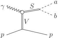
Figure 1: Vector-meson-exchange (VME) diagrams for the reaction $\gamma p\to Sp\to(ab)p$. Wavy, solid and dashed lines correspond to the photon, nucleons and final $a$ and $b$ mesons, respectively. Double lines correspond to scalar ($S$) and vector ($V$) mesons.

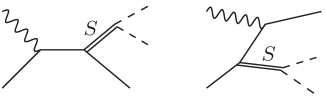
Figure 2: Born diagrams for the photoproduction reaction $\gamma p\to Sp\to(ab)p$ of neutral scalars $S=a^{0}_{0},\,f_{0}$. See the notations in Fig. 1.

Different models for $a_{0}$- and $f_{0}$-meson production can be considered. One is that derived by Oset and coauthors [27] (see also Refs. [22, 26] and references therein) and based on the chiral unitary approach. Another model was proposed in Ref. [28], in which scalar mesons are produced via the vector-meson-exchange (VME) mechanism ($\rho$ and $\omega$ exchanges). The corresponding diagrams are depicted in Fig. 1. This model, considered as a tool to extract the radiative decays of scalars to $\rho$ and $\omega$, was proposed for CLAS $\gamma p$ experiments at high photon-beam energies $E_{\gamma}\sim$ several GeV. In the case of $a_{0}(980)$ and $f_{0}(980)$ production near threshold ($E_{\gamma}\sim 1.5-1.6$ GeV), one may also expect sizable contributions from the Born diagrams shown in Fig. 2.

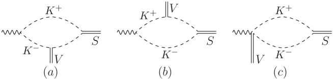
Figure 3: Loop diagrams for $SV\gamma$ vertex. Dashed lines correspond to charged $K^{\pm}$ mesons. Other curves mean the same as in Fig. 1.

The diagrams in Fig. 1 contain an essential ingredient, i.e., the radiative decay $SV\gamma$ vertices ($S=a_{0},f_{0}$; $V=\rho,\omega$), which can be estimated in different ways. This is the main source of uncertainties when calculating the diagrams. Firstly, $SV\gamma$ vertices can be estimated from quark model, fitted to data on the radiative widths; however, the results strongly depend on the quark structure of the scalars, which is not known exactly. Another approach is the dynamical model for $SV\gamma$ coupling via intermediate hadronic states. Here, the main contribution in the case of $a_{0}(980)$ and $f_{0}(980)$ comes from the kaon-loop diagrams, shown in Fig. 3, which are proportional to the $a_{0}K\bar{K}$ or $f_{0}K\bar{K}$ coupling constants. The Born diagrams in Fig. 2 depend on the $a_{0}N\!N$ and $f_{0}N\!N$ coupling constants, also known with large uncertainty.

Further, we consider separately the above-mentioned models and write down the amplitudes. We use the following notation: $q$, $p_{1}$($p_{2}$), and $k$ are the four-momenta of the initial photon, initial (final) proton, and final scalar meson $S$, respectively; $\epsilon$ is the photon polarization four-vector; $(pq)$ is the scalar product of four-vectors $p$ and $q$; $\hat{p}\equiv p_{\mu}\gamma^{\mu}$.

2.1 Model A

The amplitude $M$ of the reaction $\gamma p\!\to\!pab$ is constructed from the VME diagrams in Fig. 1 and reads

$$M=\sum_{s=a_{0},f_{0}}M_{S},~{}~{}~{}~{}M_{S}=\sum_{V=\rho,\omega}\frac{1}{t-m^{2}_{V}}\,\Gamma_{\mu}\,\bar{u}_{2}\hat{F}^{\mu}u_{1}\,G_{S}(W)\,g_{sab},$$ (1)

where $M_{S}$ is the amplitude of $S$-meson photoproduction in the $ab$ channel ($ab=\pi\eta,\,\pi\pi,\,K\bar{K}$). Here: $\Gamma_{\mu}$ is the $SV\gamma$ vertex of general (gauge invariant) form

$$\Gamma_{\mu}=I_{sv\gamma}\,[(qk)e_{\mu}-(ek)q_{\mu}],$$ (2)

related to the radiative decay width as

$$\Gamma(S\to\gamma V)=|I_{sv\gamma}|^{2}\frac{m^{3}_{S}}{32\pi}\left(1-\frac{m^{2}_{V}}{m^{2}_{S}}\right)^{3},$$ (3)

where $m_{V}$ ($m_{S}$) is the mass of vector (scalar) meson; $F_{\mu}$ is the $VNN$ vertex and

$$F_{\mu}=g_{V}\gamma_{\mu}+if\!_{V}\sigma_{\mu\nu}p_{\nu}~{}~{}(p=p_{2}-p_{1}),$$ (4)

where $g_{V}$ ($f\!_{V}$) is vector (tensor) $V\!N\!N$ coupling constant; $u_{1,2}$ are Dirac spinor of the initial and final nucleons ($\bar{u}u=2m$, where $m$ is the nucleon mass); $G_{S}(W)$, $g_{sab}$ and $W$ are the $S$-meson propagator, $Sab$-coupling constant and effective mass of meson $ab$ system (the expression for $G_{S}(W)$ and definition for $g_{sab}$ are given in Appendix A.1). The vector-meson propagator in Eq. (1) is taken as the simple form $1/(t-m^{2}_{V})$, where $t=(p_{2}-p_{1})^{2}$, instead of the reggeized prescription used in Ref. [28], since we consider the photoproduction of scalar mesons in the threshold region. For the $V\!N\!N$ constants ($V\!=\!\rho,\omega$) in Eq. (4) we use the values

$$g_{\rho}=3.4,~{}~{}f_{\rho}=11~{}{\rm GeV}^{-1},~{}~{}~{}g_{\omega}=15,~{}~{}f_{\omega}=0.$$ (5)

These values were used in Ref. [28] and are consistent with the description of pion photoproduction [29].

In the usual definitions the differential cross sections for $\gamma p\to(ab)p$ reads

$$\frac{d^{2}\sigma}{dWd\Omega}=\frac{\overline{|M|^{2}}q_{ab}Q}{(4\pi)^{4}Q_{1\,}s},~{}~{}~{}~{}~{}\frac{d^{2}\sigma}{dWdt}=\frac{\overline{|M|^{2}}q_{ab}}{4(4\pi)^{3}Q^{2}_{1\,}s}.$$ (6)

Here, $\overline{|M|^{2}}$ is the modulus squared of the amplitude for the unpolarized beam photon and nucleons, and its expression obtained from Eqs. (1)-(4) is given in Appendix A.2; $d\Omega$ is the solid-angle element of the outgoing $ab$ system in the reaction rest frame; $s=m(m+2E_{\gamma})$ is the CM total energy squared, $q_{ab}$ is the relative momentum in the $ab$ system; $Q_{1}$ ($Q$) is the momentum of the initial photon (final $ab$ system) in the reaction rest frame; the additional factor $\frac{1}{2}$ is implied in the case with identical final-state mesons $a$ and $b$. The differential cross section  (6) is written for the final $ab$ system in the $s$-wave.

In this model, the factor $I_{sv\gamma}$ in Eq. (2) is assumed to be constant. We use the width $\Gamma(S\to\gamma V)$ in Eq. (3) as input to obtain the factor $I_{sv\gamma}$.

2.2 Model B

In this variant, we use the loop mechanism with intermediate hadrons to calculate the vertex $\Gamma_{\mu}$ (2) and factor $I_{sv\gamma}$. For the scalars $a_{0}(980)$ and $f_{0}(980)$, both connected with $K\bar{K}$ channel, the dominant contribution comes from the $K\bar{K}$-loop diagrams ($a$), ($b$), and ($c$) shown in Fig. 3. The diagrams $(a)$ and ($b$) give equal contributions. The third term ($c$), which contains the $\gamma V\!KK$ vertex, is prescribed by gauge invariance. Also due to this term, the divergencies of the loop diagrams in Fig. 3 are totally cancelled, and one arrives at a finite expression for the vertex $\Gamma_{\mu}$ (2). Note that the result can be obtained, calculating the term, proportional to $(ek)q_{\mu}$ in Eq. (2), which comes from diagrams ($a$) and ($b$) and is convergent. Calculations were done in Refs. [5, 8] and give

$$I_{sv\gamma}=\frac{eg_{SK^{+}K^{-}}g_{VK^{+}K^{-}}}{2\pi^{2}m^{2}_{K}}\,I(a,b),~{}~{}~{}~{}a=\frac{m^{2}_{V}}{m^{2}_{K}},~{}~{}~{}b=\frac{m^{2}_{S}}{m^{2}_{K}}.$$ (7)

Here, $e$ is the electron charge ($e^{2}/4\pi\approx 1/137$); $g_{SK^{+}\!K^{-}}$ and $g_{V\!K^{+}\!K^{-}}$ are the coupling constants of scalar ($S$) and vector ($V$) mesons to the $K^{+}K^{-}$ channel; $m_{K}$ is the charged kaon mass. The function $I(a,b)$ comes from the calculation of the loop integral and is given in Appendix A.3. In the case of VME diagram in Fig. 1, the vector-meson mass squared $m^{2}_{V}$ is replaced by the four-momentum transfer $t$, i.e., $a=t/m^{2}_{K}$ in Eq. (7).

The constants $g_{SK^{+}K^{-}}$ are taken from Refs. [30, 31], and are given in Appendix A.1. For the values of the couplings $g_{VK^{+}K^{-}}$, we use predictions from SU(3) symmetry. Thus,

$$g_{\rho K^{+}K^{-}}=g_{\omega K^{+}K^{-}}=\frac{1}{2}\,g_{\rho\pi\pi},~{}~{}~{}~{}\Gamma(\rho\!\to\!\pi\pi)=\frac{g^{2}_{\rho\pi\pi}q^{3}_{\pi\pi}}{24\pi m^{2}_{\rho}}.$$ (8)

Here, the constant $g_{\rho\pi\pi}$ is determined in a usual way through the width and mass of the $\rho$ meson, taken from PDG [32].

2.3 Model C

We also estimate the cross sections from Born diagrams of $a_{0}/f_{0}$ photoproduction, shown in Fig. 2. The amplitude reads

$$M=\bar{u}_{2}\left[a_{s}(\hat{p}_{1}\!+\hat{q}+m)\hat{\epsilon}\,+\,a_{u}\hat{\epsilon}(\hat{p}_{1}\!-\hat{k}+m)\right]u_{1},$$ (9)

where

$$a_{s}=\frac{eC}{s-m^{2}},~{}~{}a_{u}=\frac{eC}{u-m^{2}},~{}~{}C=\sum_{s=a_{0},f_{0}}g_{s\!N}g_{sab}G_{S}(W),$$

$$s=(p_{1}+q)^{2},~{}~{}u=(p_{1}-k)^{2},$$

The amplitude is sensitive to the $a_{0}N\!N$ and $f_{0}N\!N$ coupling constants $g_{sN}$ ($s=a_{0},f_{0}$), which are known with large uncertainty. For our estimations we take some “typical” values [33]

$$g_{a_{0}N\!N}\simeq g_{f_{0}N\!N}\simeq 5.$$ (10)

The amplitude squared $\overline{|M|^{2}}$ for unpolarized photon and nucleons is given in Appendix A.2 by Eq. (A.10).

2.4 Adding of $a_{0}\!-\!f_{0}$ mixing

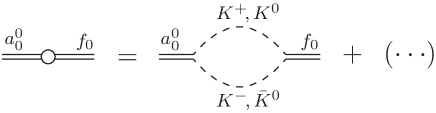
Figure 4: Diagrammatic representation for $a_{0}-f_{0}$ vertex. The notation $(\cdots)$ denotes the contributions not connected with kaon-loop mechanism and neglected here.

The leading isospin-breaking (IB) effect comes from $a_{0}-f_{0}$ mixing. Both scalars are coupled to the $K\bar{K}$ channel, and their masses are close to the $K\bar{K}$-threshold. Thus, the contribution to $a_{0}\!\leftrightarrow\!f_{0}$ transition amplitude comes from the mass difference of charged and neutral kaons and exhibits a sharp maximum in the 8-MeV mass interval between the $K^{+}K^{-}$ and $K^{0}\bar{K}^{0}$ thresholds. The effect is enhanced since it occurs in the vicinity of the $a_{0}$ and $f_{0}$ masses. The $a_{0}-f_{0}$ vertex is shown diagrammatically in Fig. 4. Here, the notation $(\cdots)$ stands for possible terms not connected with the $KK$ loop, assumed to have a smooth mass dependence. These terms admix contributions from $f_{0}(a_{0})$ to $a_{0}(f_{0})$ signals, and seem to be not identified accurately from photoproduction experiments due to the proximity of the $a_{0}$ and $f_{0}$ parameters. On the other hand, the $KK$-loop term, due to its sharp behaviour, should exhibit a visible signal in the effective mass spectra in the $a_{0}$- and $f_{0}$-decay channels. The $a_{0}f_{0}$ vertex $\lambda$, associated with the $KK$-loop diagram in Fig. 4, reads

$$\lambda=i\,\frac{g_{a_{0}K^{+}\!K^{-}}\,g_{f_{0}K^{+}\!K^{-}}}{16\pi m_{K}}\,(q_{K^{+}K^{-}}-q_{K^{0}\bar{K}^{0}}),~{}~{}~{}~{}m_{K}\!=\frac{1}{2}(m_{K^{0}}\!+m_{K^{+}}\!),$$ (11)

$$q_{K^{+}K^{-}}=\sqrt{m_{K}(W\!-2m_{K^{+}})+i0},~{}~{}~{}~{}q_{K^{0}\bar{K}^{0}}=\sqrt{m_{K}(W\!-2m_{K^{0}})+i0}.$$

The value $|\lambda|$ is maximal at $m_{K^{+}}\!<\!W\!\!<\!m_{K^{0}}$, where $|\lambda|=\frac{g_{a_{0}K^{+}\!K^{-}}\,g_{f_{0}K^{+}\!K^{-}\!}}{8\pi}\sqrt{\frac{m_{K^{0}}\!-m_{K^{+}}}{2m_{K}}}$, and rapidly decreases beyond this range.

One may include $a_{0}-f_{0}$ mixing by replacing the coupling constants $g_{sab}$ of the scalars to meson $ab$ channels by modified values $\bar{g}_{sab}$ according to the relations

$$\bar{g}_{a_{0}ab}=g_{a_{0}ab}-\lambda G_{f}\,\bar{g}_{f_{0}ab},~{}~{}~{}~{}~{}\bar{g}_{f_{0}ab}=g_{f_{0}ab}-\lambda G_{a}\,\bar{g}_{a_{0}ab},$$ (12)

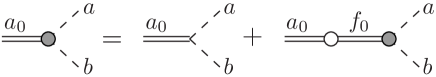
Figure 5: Diagrammatic representation for rederfined couplings $\bar{g}_{a_{0}ab}$ and $\bar{g}_{f_{0}ab}$ (gray circles), including $a_{0}-f_{0}$ mixing. The 2-nd equation (not shown) mean the replacement $a_{0}\leftrightarrow f_{0}$.

which are shown diagrammatically in Fig. 5. From Eqs. (12), we arrive at

$$\bar{g}_{a_{0}ab}\!=(g_{a_{0}ab}-\!\lambda G_{f}\,g_{f_{0}ab})Z^{-1},~{}~{}~{}\bar{g}_{f_{0}ab}\!=(g_{f_{0}ab}-\!\lambda G_{a}\,g_{a_{0}ab})Z^{-1},~{}~{}~{}Z=1\!-\!\lambda^{2}G_{a}G_{f}.$$ (13)

At $Z=1$, Eqs. (13) include only leading-order terms in the $a_{0}f_{0}$ vertex $\lambda$. The redefined vertices $\bar{g}_{sab}$ as well as the factors $G_{a}$, $G_{f}$ and $\lambda$, depend on the mass $W$, i.e., $\bar{g}_{sab}\equiv\bar{g}_{sab}(W)$.

3. Results

Here, we present some results for the total cross sections and effective $ab$-mass spectra in different channels $\gamma p\to(ab)p$ , estimated in the models of Section 2. We calculate only resonance amplitudes, i.e., the final $ab$ system is produced from $a_{0}/f_{0}$ decays, and neglect any possible background terms to the $\gamma p\to(ab)p$ amplitudes. However, it is interesting to compare the results for the cross sections obtained using different approaches.

3.1 Cross sections

First, we obtain the predictions from Model A; then, we have the radiative widths $\Gamma(S\to\gamma V)$ to input into the calculation of the $SV\gamma$ vertices $I_{sv\gamma}$ in Eq. (2). Here, we may use the results from the quark model used in Ref. [28]. In this model, assuming the $a_{0}$ and $f_{0}$ mesons to be $q\bar{q}\,(^{3}P_{0})$ states, one obtains results which depend on the $q\bar{q}$ flavor configuration. For the isovector state $a^{0}_{0}=(u\bar{u}-d\bar{d})/\sqrt{2}$  this gives

$$\Gamma(a_{0}\to\gamma\omega)=125~{}{\rm keV},~{}~{}~{}\Gamma(a_{0}\to\gamma\rho)=\frac{1}{9}\,\Gamma(a_{0}\to\gamma\omega)=14~{}{\rm keV}.$$ (14)

Considering three different $q\bar{q}$ configurations for the isoscalar $f_{0}$ meson, denoted as

$$f_{0}(1)=\frac{1}{\sqrt{2}}\,(u\bar{u}\!+\!d\bar{d}),~{}~{}f_{0}(2)=\frac{1}{\sqrt{6}}\,(u\bar{u}\!+\!d\bar{d}\!-\!2s\bar{s}),~{}~{}f_{0}(3)=\frac{1}{\sqrt{3}}\,(u\bar{u}\!+\!d\bar{d}\!+\!s\bar{s}),$$ (15)

one has

$$\begin{array}[]{l}\Gamma(f_{0}(1)\!\to\!\gamma\rho)=3\,\Gamma(f_{0}(2)\!\to\!\gamma\rho)=\frac{3}{2}\Gamma(f_{0}(3)\!\to\!\gamma\rho)=\Gamma(a_{0}\!\to\!\gamma\omega),\\ \rule{0.0pt}{16.0pt}\Gamma(f_{0}(1)\!\to\!\gamma\omega)=3\,\Gamma(f_{0}(2)\!\to\!\gamma\omega)=\frac{3}{2}\Gamma(f_{0}(3)\!\to\!\gamma\omega)=\Gamma(a_{0}\!\to\!\gamma\rho).\end{array}$$ (16)

The case $f_{0}=s\bar{s}$ gives $\Gamma(f_{0}\!\to\!\gamma\rho/\omega)\sim\sin^{2}\theta$, where $\theta$ is the $\phi-\omega$-mixing angle. The angle $\theta$ is assumed to be small and this case is not considered here.

The cross sections $\sigma(ab)$ (in $\mu b$) for different channels are shown in Table 1. The results of Model A are given for three variants 1), 2), and 3), where $f_{0}$ is taken as the $f_{0}(1)$, $f_{0}(2)$ and $f_{0}(3)$ states, respectively. The cross section $\sigma(\pi^{0}\eta)$ slightly depends on the variants of the $f_{0}$ states (15) due to $a_{0}-f_{0}$ mixing, while the main contribution comes from the $a_{0}$-production amplitudes. The cross sections $\sigma(\pi\pi)$ are mainly determined by the $f_{0}$-production terms, and are more sensitive to the $f_{0}$ variants (15). Models B and C give comparable values for the cross section but much smaller ones than those obtained from Model A.

For some comparison with existing data we present in Fig. 6 the cross section $\sigma(\pi^{0}\eta)$ versus total centre-of-mass energy $\sqrt{s}=W(\gamma p)$ in Model B for two sets of $a_{0}/f_{0}$ parameters (solid and dashed curves, see figure caption). Here, open circles show the $a_{0}(980)p$ contribution to the $\pi^{0}\eta p$ channel, obtained through a partial-wave analysis (PWA) of the data on $\gamma p\to\pi^{0}\eta p$ in Ref. [34]. Thus, the model results essentially depend on $a_{0}/f_{0}$ parameters, but Model B is in rough agreement with the “data” (open circles). The cross sections from Model A are too large and not shown in Fig. 6. Note also that $W(\gamma p)=1.97$ GeV for the energy of interest $E_{\gamma}=1.6$ GeV.

Concerning the other channels, there are recent CLAS high-statistics data on the reaction $\gamma p\to\pi^{+}\pi^{-}p$ at $E_{\gamma}=3.0-3.8$ GeV [35]. The PWA results of Ref. [35] give, in particular, the contribution of the $s$-wave system $(\pi^{+}\pi^{-})_{s}$ with clear evidence of the $f_{0}(980)$ structure. One should also mention the old hydrogen $\gamma p\to K^{+}K^{-}p$ data [36], where the $s$-wave $(K^{+}K^{-})_{s}$ cross section and possible contributions of a scalar resonance ($M_{\pi\pi}\sim 1$ GeV) were estimated.

Generally, the photoproduction processes of scalars should be analyzed in the full approach which incorporates the resonance and background terms and utilizes unitarity. For example, the background tree $\rho,\omega$-exchange amplitudes for $\pi\pi$, $\pi\eta$, and $\eta\eta$ channels were taken into account in Ref. [28], and their contribution was found to be comparable with the resonance terms in the corresponding mass intervals. Analogous tree amplitudes supplemented with $s$-wave meson-meson final state interaction (FSI) were considered for the $\pi\pi$ and $K\bar{K}$ photoproduction in Refs. [37], where the cross sections for $s$-wave $(\pi\pi)_{s}$ and $(K\bar{K})_{s}$ pairs were estimated.

In the present paper, we leave the inclusion of such background processes for future work and study the $a_{0}-f_{0}$-mixing effect which is produced by the resonance amplitudes.

3.2 Mass spectra

The results for the total cross sections given in Table 1 exhibit a strong model dependence, but are only weakly sensitive to the $a_{0}-f_{0}$ mixing. As mentioned above, the $a_{0}f_{0}$ vertex $\lambda$ (11) sharply depends on the mass $W$ and peaks close to the $K\bar{K}$ thresholds.

The mass spectra for the two channels $\pi^{0}\eta$ and $\pi^{+}\pi^{-}$ at the beam-photon energy $E_{\gamma}=1.6$ GeV are presented in Fig. 7. The results are given for two models, A (variant 1) and B with the $a_{0}/f_{0}$ parameters from the “KK” version (see, Eqs. (A.4)). All the plots in Fig. 7 exhibit two kinds of phenomena: the “cusp” effects at the $K\bar{K}$ thresholds and $a_{0}-f_{0}$-mixing. The latter is seen as the differences of solid and dashed curves. The “cusp” effects look more pronounced in the $\pi\pi$ channel than in the $\pi\eta$ one, essentially because the $f_{0}$ has larger coupling to the $K\bar{K}$ channels than the $a_{0}$.

Models A and B in Fig. 7 give quite similar shapes of mass spectra. To get some view of model dependence of the results, we present some other predictions for the same channels in Fig. 8. The plots $a$ and $b$ show the mass spectra obtained in Model A (variant 2, i.e., $f_{0}=f_{0}(2)$ in Eq. (15)) with the same “KK” variant of the $a_{0}/f_{0}$ parameters. Here, since the radiative widths $\Gamma(f_{0}\!\to\!\gamma\rho/\omega)$ for $f_{0}(2)$ is 3 times smaller than for $f_{0}(1)$, the $d\sigma/dM(\pi\pi)$ is also getting $\sim 3$ smaller in comparison with that in plot $b$ of Fig. 7.

The plots $c$ and $d$ in Fig. 8 show the results from Model A (variant 1), but with the no-structure (“NS”) variant of the $a_{0}/f_{0}$ parameters. In the “NS” version, both constants $g_{aK^{+}K^{-}}$ and $g_{fK^{+}K^{-}}$ are smaller (the latter by $\sim$ one order of magnitude) than their “KK”- version values (see Eqs. (A.4)). Thus, the “cusp” effects as well as the $a_{0}-f_{0}$-mixing (note that the $a_{0}f_{0}$ vertex (11) $\lambda\sim g_{aK^{+}K^{-}}g_{fK^{+}K^{-}}$) are hardly visible in this case.

Fig. 9 shows the effective $K^{+}K^{-}$ mass spectra in the reaction $\gamma p\!\to\!(K^{+}K^{-})p$ at the same photon energy. Here we give the results of the same four variants of the model calculations as in Figs. 7 and 8 (see figure caption). Plot $d$ shows the results obtained with the “NS” version of the $a_{0}/f_{0}$ parameters. $a_{0}-f_{0}$-mixing is also suppressed here due to smaller couplings of the resonances to the $K\bar{K}$ channels. Thus, we see that the IB $a_{0}-f_{0}$-mixing effect essentially depends on the $a_{0}/f_{0}$ parameters, in particular on the $a_{0}$ and $f_{0}$ couplings to the $K\bar{K}$ channel.

From an experimental point of view, one can not measure the reaction discussed with “switched off” isospin-breaking effects in order to observe any difference in the mass spectra like those between the solid and dotted curves in Figs. 7-9. Thus, we also need to study the charged channels, where mixing is absent, say, $a^{+}_{0}$ photoproduction in $\gamma p\!\to\!(\pi^{+}\eta)n$, in parallel with the neutral channels to compare the results.

4. Conclusion

The photoproduction of the neutral scalars $a_{0}(980)$ and $f_{0}(980)$ on a proton target at energies close to threshold were considered in the $\pi\eta$, $\pi\pi$, and $K\bar{K}$ channels. The main aim of the paper is to study the possibility of observing $a_{0}-f_{0}$ mixing in these processes. Several models of $a_{0}/f_{0}$ photoproduction were considered with $a_{0}-f_{0}$ mixing included through the $K\bar{K}$-loop mechanism of $a_{0}-f_{0}$ transition. The total cross sections of different channels were estimated and appeared to be very model dependent. Model B, incorporating $\rho$ and $\omega$-exchange diagrams and a $K\bar{K}$-loop mechanism for $a_{0}/f_{0}$ photoproduction, demonstrates rough agreement with the data on the $a_{0}$ contribution to the $\gamma p\to\pi^{0}\eta p$ cross section.

The two-meson mass spectra are examined for observation of $a_{0}-f_{0}$-mixing. The most interesting case is the $\gamma p\to\pi^{0}\eta p$ channel. Here, the $\pi^{0}\eta$-effective-mass spectrum demonstrates a sharp (mixing) effect (Fig. 7), i.e., rapid behavior of the $d\sigma/dM$ in the narrow ($\sim 8$ MeV) mass interval, for the case of $a_{0}/f_{0}$ parameters, taken from “kaon loop” fits of Refs. [30, 31]. The effect is sensitive to the $a_{0}/f_{0}$ parameters.

Both aspects, the $SV\gamma$ vertex $I_{sv\gamma}$ (see Eq. (2)), which affects the photoproduction cross section of scalars, and the $a_{0}-f_{0}$-mixing vertex $\lambda$ (11), are important to understand the nature of scalar mesons $a_{0}(980)$ and $f_{0}(980)$. We expect this study to be continued in a more complete model, incorporating also the background amplitudes for the given channels.

Acknowledgments

The authors are thankful to M. Amaryan and S. Prakhov for many useful discussions concerning the experimental possibilities to measure $a_{0}/f_{0}$ photoproduction and E. Oset for useful references. This work was supported in part by the U.S. Department of Energy Grant No. DE–FG02–99ER41110 and the DFG under grant SFB 1044. A. E. K. thanks grant NS–3172.2012.2 for partial support.

Appendix

A.1 Scalar meson propagators

The propagators of scalars reads

$$G_{S}=(W^{2}-m^{2}_{S}+iW\,\Gamma_{S}(W))^{-1},~{}~{}~{}~{}\Gamma_{S}(W)=\sum_{ab}\Gamma_{sab}(W).$$

The total width $\Gamma_{S}(W)$ is the sum of partial widths $\Gamma_{sab}(W)$ of the $s$-wave decays $S\!\to\!ab$, and

$$\Gamma_{\!sab}(W)=\frac{g^{2}_{sab}q_{ab}}{8\pi W^{2}},~{}~{}~{}~{}~{}ab=\biggl{\{}\begin{array}[]{ll}\pi^{0}\eta,\,K^{+}\!K^{-}\!,\,K^{0}\bar{K}^{0}&(S=a^{0}_{0})\\ \pi\pi\!,~{}~{}\,K^{+}\!K^{-}\!,\,K^{0}\bar{K}^{0}&(S=f_{0})\end{array}.$$

Here, $g_{sab}$ is the coupling constant of the scalar $S$ to $ab$ channel;

$$q_{ab}=\sqrt{\frac{1}{4W^{2}}\,(W^{2}\!-m^{2}_{+})(W^{2}\!-m^{2}_{-})+i0},~{}~{}~{}~{}~{}m_{\pm}=m_{a}\pm m_{b},$$

where $q_{ab}$ is the relative momentum in the $ab$ system with effective mass $W$, and $m_{a}$ ($m_{b}$) is the mass of particle $a$ ($b$). The value $q_{ab}$ in Eq. (A.3) is also defined in the region below threshold, i.e., $q_{ab}=i|\,q_{ab}|$ at $W\!<\!m_{a}\!+\!m_{b}$.

The $a_{0}(980)$ and $f_{0}(980)$ parameters are taken from the analyses of $\phi(1020)\!\to\!\pi^{0}\eta\gamma$ [30] and $\phi\!\to\!\pi^{0}\pi^{0}\gamma$ [31]. The results were obtained for two variants of fits – “kaon loop” (“KK”) and “no structure” (“NS”) models:

$$\begin{array}[]{llcl}{\rm``KK"}\!\!:&m_{a}\!=983~{}{\rm MeV},&g_{a\pi\eta}=2.8~{}{\rm GeV},&g_{aK^{+}K^{-}}\!=2.16~{}{\rm GeV};\\ \rule{0.0pt}{16.0pt}{\rm``KK"\!\!}:&m_{f}\!=976.8~{}{\rm MeV},&g_{f\pi^{+}\pi^{-}}\!=-1.43~{}{\rm GeV},&g_{fK^{+}K^{-}}\!=3.76~{}{\rm GeV};\\ \rule{0.0pt}{16.0pt}{\rm``NS":}&m_{a}\!=983~{}{\rm MeV},&g_{a\pi\eta}=2.2~{}{\rm GeV},&g_{aK^{+}K^{-}}\!=1.57~{}{\rm GeV};\\ \rule{0.0pt}{16.0pt}{\rm``NS"}\!:&m_{f}\!=984.7~{}{\rm MeV},&g_{f\pi^{+}\pi^{-}}\!=1.31~{}{\rm GeV},&g_{fK^{+}K^{-}}\!=0.40~{}{\rm GeV}\end{array}$$

($g_{aK^{0}\bar{K}^{0}}\!=-g_{aK^{+}K^{-}}$,  $g_{fK^{0}\bar{K}^{0}}\!=g_{fK^{+}K^{-}}$).

A.2 Reaction amplitude squared

Models A,B. The reaction amplitude $M$ can be written as

$$M=\bar{u}_{2}(A+\hat{B})u_{1},$$

where

$$A=a_{1}[(\epsilon k)(q,p_{1}+p_{2})-(qk)(\epsilon,p_{1}+p_{2})],~{}~{}~{}~{}\hat{B}=a_{3}[(\epsilon k)\hat{q}-(qk)\hat{\epsilon}],$$

$$a_{1}=\sum_{S,V}\frac{G_{S}\,g_{sab}f_{V}}{t-m^{2}_{V}}\,I_{SV},~{}~{}~{}a_{2}=\sum_{S,V}\frac{G_{S}\,g_{sab}g_{V}}{t-m^{2}_{V}}\,I_{SV},~{}~{}~{}a_{3}=2ma_{1}+a_{2}.$$

The modulus squared of the amplitude for unpolarized particles reads

$$\overline{|M|^{2}}=\frac{1}{2}\,{\rm Tr}\,\{(A^{*}\!+\hat{B}^{*})(\hat{p}_{2}\!+m)((A\!+\hat{B})(\hat{p}_{1}\!+m)\}~{}~{}~{}(\hat{B}^{*}\!\equiv B^{*}_{\mu}\gamma^{\mu}),$$

where the trace Tr$\{\cdots\}$ is averaged over photon polarizations. To simplify calculations we impose gauge condition $\epsilon_{0}\!=\epsilon_{3}\!=0$ on the photon four-vector $\epsilon$. Thus, the total set of useful scalar products with four-vector $\epsilon$ is

$$(\epsilon q)=(\epsilon p_{1})=0,~{}~{}(\epsilon p_{2})=-(\epsilon k)=(\mbox{\boldmath$\epsilon$}\mbox{\boldmath$k$}_{\perp}),~{}~{}\epsilon^{2}=-1.$$

Finally, from Eq. (A.6), making use of Eq. (A.7), we arrive at

$$\overline{|M|^{2}}=2(\,|\,a_{2}|^{2}\!-|\,a_{1}|^{2}t)(qp_{1\!})^{2}k^{2}_{\perp}-|\,a_{3}|^{2}(qk)^{2}t,$$

where substitution $(\epsilon k)^{2}\to\frac{1}{2}k^{2}_{\perp}$ is used for unpolarized photon. The factors $(qp_{1\!})^{2}k^{2}_{\perp}$ and $(qk)^{2}$ in Eq. (A.8) can be written as

$$(qp_{1\!})^{2}k^{2}_{\perp}=\frac{1}{4}s(t_{2}-|t|)(|t|-t_{1}),~{}~{}~{}~{}(qk)^{2}=\frac{1}{2}(W^{2}-t),$$

where $t_{1}$ and $t_{2}$ are the kinematical boundaries for $|t|$ ($t_{1}\!<\!|t|\!<\!t_{2}$).

Model C. Making use of Eqs. (A.7) and Dirac equations for nucleon spinors $u_{1}$ and $\bar{u}_{2}$, one can rewrite the amplitude in Eq. (9) in the form

$$M=\bar{u}_{2}\left[\,2a_{u}(\epsilon p_{2})+(a_{s}+a_{u})\,\hat{q}\hat{\epsilon}\,\right]u_{1}.$$

Calculations for unpolarized particles give

$$\overline{|M|^{2}}=4\left[\,|\,a_{s}\!+\!a_{u}|^{2}(qp_{1})(qp_{2})+k^{2}_{\perp}[\,|\,a_{u}|^{2}(m^{2}\!+(p_{1},p_{2}\!-q))-{\rm Re}(a^{+}_{s}a_{u})(qp_{1})]\right].$$

A.3 Loop function $I(a,b)$

The loop function $I(a,b)$, which enters the $SV\gamma$ vertex $I_{svg}$ in Eq. (7), can be written as the integral

$$I(a,b)=\int\limits^{1}_{0}dz\int\limits^{1-z}_{0}dy\frac{yz}{c-i0},~{}~{}~{}c=1-z(1-z)a-yz(b-a).$$

Calculations give (see, also [5, 28])

$$I(a,b)=\frac{1}{2(a-b)}+\frac{a}{2(a-b)^{2}}\,[J(b)-J(a)]+\frac{1}{2(a-b)^{2}}\,[f(b)-f(a)],$$

where

$$\begin{array}[]{lll}1)~{}J(a)=x(L-i\pi),&f(a)=-(L-i\pi)^{2},&(a>4);\\ \rule{0.0pt}{16.0pt}2)~{}J(a)=2xA,&f(a)=4A^{2},&(0<a<4);\\ \rule{0.0pt}{16.0pt}3)~{}J(a)=xL,&f(a)=-L^{2},&(a<0);\end{array}$$

$$x=\sqrt{\left|\frac{a-4}{a}\right|},~{}~{}~{}L=\ln\left|\frac{1+x}{1-x}\right|,~{}~{}~{}A=\arcsin\frac{\sqrt{a}}{2}.$$

References

Figure 6: Total cross section for $\gamma p\to a^{0}_{0}p\to\pi^{0}\eta p$ versus total centre-of-mass energy $W(\gamma p)$. The curves show the results from the Model B ($a_{0}-f_{0}$ mixing is included). The results are given for two sets of $a_{0}/f_{0}$ parameters, taken from Refs. [30, 31] – “kaon loop” fit (solid curve) and “no structure” fit (dashed curve) (see Eq. (A.4)). Open circles show the $a_{0}p$ contribution to the $\gamma p\to\pi^{0}\eta p$ cross section extracted through PWA in Ref. [34].

Figure 7: The mass distributions $d\sigma/dM(\pi^{0}\eta)$ (plots $a$ and $c$) and $d\sigma/dM(\pi^{+}\pi^{-})$ (plots $b$ and $d$) in the reactions $\gamma p\to(\pi^{0}\eta)p$ and $\gamma p\to(\pi^{+}\pi^{-})p$, respectively, at $E_{\gamma}=1.6$ GeV. The plots $a$ and $b$ show the results from the Model A with variant $f_{0}=f_{0}(1)$ (15); the plots $c$ and $d$ – the results from the Model B. Solid (dashed) curves show the results obtained with $a_{0}-f_{0}$ mixing included (excluded). The $a_{0}/f_{0}$ parameters are taken from Refs. [30, 31] (“kaon loop” fits). Vertical dotted lines point the $K\bar{K}$-threshold positions.

Figure 8: The mass distributions $d\sigma/dM(\pi^{0}\eta)$ (plots $a$ and $c$) and $d\sigma/dM(\pi^{+}\pi^{-})$ (plots $b$ and $d$), respectively. The reactions are the same as in Fig. 7, and $E_{\gamma}=1.6$ GeV. The plots $a$ and $b$ show the results from the Model A with variant $f_{0}=f_{0}(2)$ (15) with the $a_{0}/f_{0}$ parameters from Refs. [30, 31] (“kaon loop” fits); the plots $c$ and $d$ – the results from the Model A with variant $f_{0}=f_{0}(1)$ (15) with the $a_{0}/f_{0}$ parameters from Refs. [30, 31] (“NS” fits). Notations of the curves are the same as in Fig. 7.

Figure 9: The mass distributions $d\sigma/dM(K^{+}K^{-})$ in the reaction $\gamma p\to(K^{+}K^{-})p$ at $E_{\gamma}=1.6$ GeV. The plots: $a,d$ – model A with variant $f_{0}=f_{0}(1)$ (15); $b$ – Model B; $c$ – Model A with variant $f_{0}=f_{0}(2)$ (15). The $a_{0}/f_{0}$ parameters are taken from Refs. [30, 31]: plots $a,b,c$ – “kaon loop” fits; $d$ – “NS” fits. Notations of the curves are the same as in Fig. 7.