The Stark problem in the Weierstrassian formalism

Abstract

We present a new general, complete closed-form solution of the three-dimensional Stark problem in terms of Weierstrass elliptic and related functions. With respect to previous treatments of the problem, our analysis is exact and valid for all values of the external force field, and it is expressed via unique formulæ valid for all initial conditions and parameters of the system. The simple form of the solution allows us to perform a thorough investigation of the properties of the dynamical system, including the identification of quasi-periodic and periodic orbits, the formulation of a simple analytical criterion to determine the boundness of the trajectory, and the characterisation of the equilibrium points.

1 Introduction

The dynamical system consisting of a test particle subject simultaneously to an inverse-square central field and to a force field constant both in magnitude and direction is known under multiple denominations. Historically, this system was first studied in detail in the context of particle physics (where it is known as Stark problem (Stark, 1914)) in connection with the shifting and splitting of spectral lines of atoms and molecules in the presence of an external static electric field.

In astrophysics and dynamical astronomy, the Stark problem is sometimes known as the accelerated Kepler problem, and it is studied in several contexts. Models based on the accelerated Kepler problem have been used to study the excitation of planetary orbits by stellar jets in protoplanetary disks and to explain the origin of the eccentricities of extrasolar planets (Namouni, 2005; Namouni & Guzzo, 2007; Namouni, 2013). The Stark problem has also been used in the study of the dynamics of dust grains in the Solar System (Belyaev & Rafikov, 2010; Pástor, 2012).

In astrodynamics, the Stark problem is relevant in connection to the continuous-thrust problem, describing the dynamics of spacecrafts equipped with ion thrusters. In such a context, the trajectory of the spacecraft is often considered as a series of non-Keplerian arcs resulting from the simultaneous action of the gravitational acceleration and the constant thrust provided by the engine (Sims & Flanagan, 1999).

From a purely mathematical perspective, the importance of the Stark problem lies mainly in fact that it belongs to the very restrictive class of Liouville-integrable dynamical systems of classical mechanics (Arnold, 1989). Action-angle variables for the Stark problem can be introduced in a perturbative fashion, as explained in Born (1927) and Berglund & Uzer (2001).

Different types of solutions to the Stark problem are available in the literature. If the constant acceleration field is much smaller than the Keplerian attraction along the orbit of the test particle, the problem can be treated in a perturbative fashion, and the (approximate) solution is expressed as the variation in time of the Keplerian (or Delaunay) orbital elements of the osculating orbit (Vinti, 1966; Berglund & Uzer, 2001; Namouni & Guzzo, 2007; Belyaev & Rafikov, 2010; Pástor, 2012). A different approach is based on regularisation procedures such as the Levi-Civita and Kustaanheimo-Stiefel transformations (Kustaanheimo & Stiefel, 1965; Saha, 2009), which yield exact solutions in a set of variables related to the cartesian ones through a rather complex nonlinear transformation (Kirchgraber, 1971; Rufer, 1976; Poleshchikov, 2004). A third way exploits the formulation of the Stark problem in parabolic coordinates to yield an exact solution in terms of Jacobi elliptic functions and integrals (Lantoine & Russell, 2011).

The aim of this paper is to introduce and examine a new solution to the Stark problem that employs the Weierstrassian elliptic and related functions. The main features of our solution can be summarised as follows:

• it is an exact (i.e., non-perturbative), closed-form and explicit solution;

• it is expressed as a set of unique formulæ independent of the values of the initial conditions and of the parameters of the system;

• it is a solution to the full three-dimensional Stark problem (whereas many previous solutions deal only with the restricted case in which the motion is confined to a plane).

The simple form of our solution allows us to examine thoroughly the dynamical features of the Stark problem, and to derive several new results (e.g., regarding questions of (quasi) periodicity and boundness of motion). Our method of solution is in some sense close to the one employed in Lantoine & Russell (2011). However, we believe that our solution offers several distinct advantages:

• by adopting the Weierstrassian formalism (instead of the Jacobian one), we sidestep the issue of categorising the solutions based on the nature of the roots of the polynomials generating the differential equations, and thus our formulæ do not depend on the initial conditions or on the parameters of the system;

• we provide explicit formulæ for the three-dimensional case;

• we avoid introducing a second time transformation in the solution.

These advantages are critical in providing new insights in the dynamics of the Stark problem. On the other hand, the use of the Weierstrassian formalism presents a few additional difficulties with respect to the approach described in Lantoine & Russell (2011), the most notable of which is probably the necessity of operating in the complex domain. Throughout the paper, we will highlight these difficulties and address them from the point of view of the actual implementation of the formulæ describing our solution to the Stark problem.

In this paper, we will focus our attention specifically on the full three-dimensional Stark problem, where the motion of the test particle is not confined to a plane, and we will only hint occasionally at the bidimensional case (where instead the motion is constrained to a plane).

2 Problem formulation

From a dynamical point of view, the Stark problem is equivalent to a one-body gravitational problem with an additional force field which is constant both in magnitude and direction. The corresponding Lagrangian in cartesian coordinates $\bm{r}=\left(x,y,z\right)$ and velocities $\bm{v}=\left(\dot{x},\dot{y},\dot{z}\right)$ is then

$$L\left(\bm{v};\bm{r}\right)=\frac{1}{2}v^{2}+\frac{\mu}{r}+\varepsilon z,$$ (1)

where the inertial coordinate system has been centred on the central body, $v=\left|\bm{v}\right|$, $r=\left|\bm{r}\right|$, $\mu$ is the gravitational parameter of the system and $\varepsilon>0$ is the constant acceleration imparted to the test particle by the force field. Without loss of generality, the coordinate system has been oriented so that the force field is directed towards the positive $z$ axis.

Following the lead of Epstein (1916) and Born (1927), we proceed by expressing the Lagrangian in parabolic coordinates $\left(\xi,\eta,\phi\right)$ via the coordinate transformation

$$x =\xi\eta\cos\phi, \dot{x} =\left(\dot{\xi}\eta+\xi\dot{\eta}\right)\cos\phi-\xi\eta\dot{\phi}\sin\phi,$$ (2)

$$y =\xi\eta\sin\phi, \dot{y} =\left(\dot{\xi}\eta+\xi\dot{\eta}\right)\sin\phi+\xi\eta\dot{\phi}\cos\phi,$$ (3)

$$z =\frac{\xi^{2}-\eta^{2}}{2}, \dot{z} =\xi\dot{\xi}-\eta\dot{\eta},$$ (4)

where $\xi\geq 0$, $\eta\geq 0$ and $\phi\in\left(-\pi,\pi\right]$ is the azimuthal angle. The inverse transformation from cartesian to parabolic coordinates is

$$\xi =\sqrt{r+z}, \dot{\xi} =\frac{\dot{r}+\dot{z}}{2\sqrt{r+z}},$$ (5)

$$\eta =\sqrt{r-z}, \dot{\eta} =\frac{\dot{r}-\dot{z}}{2\sqrt{r-z}},$$ (6)

$$\phi =\arctan\left(y,x\right), \dot{\phi} =\frac{\dot{y}x-\dot{x}y}{x^{2}+y^{2}},$$ (7)

where $\dot{r}=\left(\bm{v}\cdot\bm{r}\right)/r$ and $\arctan$ is the two-argument inverse tangent function. In the new coordinate system,

$$v^{2} =\left(\xi^{2}+\eta^{2}\right)\left(\dot{\xi}^{2}+\dot{\eta}^{2}\right)+\xi^{2}\eta^{2}\dot{\phi}^{2},$$ (8)

$$r =\frac{\xi^{2}+\eta^{2}}{2},$$ (9)

and the Lagrangian becomes

$$L=\frac{1}{2}\left[\left(\xi^{2}+\eta^{2}\right)\left(\dot{\xi}^{2}+\dot{\eta}^{2}\right)+\xi^{2}\eta^{2}\dot{\phi}^{2}\right]\\ +\frac{2\mu}{\xi^{2}+\eta^{2}}+\varepsilon\frac{\xi^{2}-\eta^{2}}{2}.$$ (10)

Switching now to the Hamiltonian formulation through a Legendre transformation, the momenta are defined as

$$p_{\xi} =\frac{\partial L}{\partial\dot{\xi}}=\left(\xi^{2}+\eta^{2}\right)\dot{\xi},$$ (11)

$$p_{\eta} =\frac{\partial L}{\partial\dot{\eta}}=\left(\xi^{2}+\eta^{2}\right)\dot{\eta},$$ (12)

$$p_{\phi} =\frac{\partial L}{\partial\dot{\phi}}=\xi^{2}\eta^{2}\dot{\phi},$$ (13)

and the Hamiltonian is written as

$$\mathcal{H} =\dot{\xi}p_{\xi}+\dot{\eta}p_{\eta}+\dot{\phi}p_{\phi}-L$$ (14)

$$=\frac{1}{2}\frac{p_{\xi}^{2}+p_{\eta}^{2}}{\xi^{2}+\eta^{2}}+\frac{1}{2}\frac{p_{\phi}^{2}}{\xi^{2}\eta^{2}}-\frac{2\mu}{\xi^{2}+\eta^{2}}-\varepsilon\frac{\xi^{2}-\eta^{2}}{2}.$$ (15)

Since the coordinate $\phi$ is absent from the Hamiltonian, the momentum $p_{\phi}$ is a constant of motion. It can be checked by substitution that $p_{\phi}$ is the $z$ component of the total angular momentum of the system. Thus, when $p_{\phi}$ vanishes, the motion is confined to a plane perpendicular to the $xy$ plane and intersecting the origin, and we can refer to this subcase as the bidimensional problem (as opposed to the three-dimensional problem when $p_{\phi}$ is not null).

We now employ a Sundman regularisation (Sundman, 1912), introducing the fictitious time $\tau$ via the differential relation

$$dt=\left(\xi^{2}+\eta^{2}\right)d\tau,$$ (16)

and the new, identically null, function

$$\mathcal{H}_{\tau}\left(p_{\xi},p_{\eta},p_{\phi};\xi,\eta,\phi\right)=\left(\mathcal{H}-h\right)\left(\xi^{2}+\eta^{2}\right),$$ (17)

where $h$ is the energy constant of the system (obtained by substituting the initial conditions into the expression of $\mathcal{H}$). We have then for $p_{\xi}$ and $\xi$

$$\frac{dp_{\xi}}{d\tau} =\frac{dp_{\xi}}{dt}\frac{dt}{d\tau}=-\frac{\partial\mathcal{H}}{\partial\xi}\left(\xi^{2}+\eta^{2}\right)=-\frac{\partial\mathcal{H}_{\tau}}{\partial\xi},$$ (18)

$$\frac{d\xi}{d\tau} =\frac{d\xi}{dt}\frac{dt}{d\tau}=\frac{\partial\mathcal{H}}{\partial p_{\xi}}\left(\xi^{2}+\eta^{2}\right)=\frac{\partial\mathcal{H}_{\tau}}{\partial p_{\xi}},$$ (19)

and, similarly for $p_{\eta}$, $\eta$, $p_{\phi}$ and $\phi$,

$$\frac{dp_{\eta}}{d\tau} =-\frac{\partial\mathcal{H}_{\tau}}{\partial\eta},$$ (20)

$$\frac{d\eta}{d\tau} =\frac{\partial\mathcal{H}_{\tau}}{\partial p_{\eta}},$$ (21)

$$\frac{dp_{\phi}}{d\tau} =-\frac{\partial\mathcal{H}_{\tau}}{\partial\phi},$$ (22)

$$\frac{d\phi}{d\tau} =\frac{\partial\mathcal{H}_{\tau}}{\partial p_{\phi}}.$$ (23)

$\mathcal{H}_{\tau}$ can thus be considered as an Hamiltonian function describing the evolution of the system in fictitious time. Explicitly,

$$\mathcal{H}_{\tau}=-\varepsilon\frac{\xi^{4}}{2}-h\xi^{2}+\frac{1}{2}p_{\xi}^{2}+\frac{1}{2}\frac{p_{\phi}^{2}}{\xi^{2}}\\ +\varepsilon\frac{\eta^{4}}{2}-h\eta^{2}+\frac{1}{2}p_{\eta}^{2}+\frac{1}{2}\frac{p_{\phi}^{2}}{\eta^{2}}-2\mu,$$ (24)

and the Hamiltonian $\mathcal{H}_{\tau}$ has thus been separated into the two independent constants of motion

$$\alpha_{1} =-\varepsilon\frac{\xi^{4}}{2}-h\xi^{2}+\frac{1}{2}p_{\xi}^{2}+\frac{1}{2}\frac{p_{\phi}^{2}}{\xi^{2}},$$ (25)

$$\alpha_{2} =\varepsilon\frac{\eta^{4}}{2}-h\eta^{2}+\frac{1}{2}p_{\eta}^{2}+\frac{1}{2}\frac{p_{\phi}^{2}}{\eta^{2}}.$$ (26)

These constants represent the conservation of a component of the generalised Runge-Lenz vector (Redmond, 1964). By inversion of $\alpha_{1}$ and $\alpha_{2}$ for $p_{\xi}$ and $p_{\eta}$, Hamilton’s equations finally yield

$$p_{\xi}=\frac{d\xi}{d\tau} =\pm\frac{1}{\xi}\sqrt{\varepsilon\xi^{6}+2h\xi^{4}+2\alpha_{1}\xi^{2}-p_{\phi}^{2}},$$ (27)

$$p_{\eta}=\frac{d\eta}{d\tau} =\pm\frac{1}{\eta}\sqrt{-\varepsilon\eta^{6}+2h\eta^{4}+2\alpha_{2}\eta^{2}-p_{\phi}^{2}},$$ (28)

$$\frac{d\phi}{d\tau} =p_{\phi}\left(\frac{1}{\xi^{2}}+\frac{1}{\eta^{2}}\right).$$ (29)

The solution of the Stark problem has thus been reduced to the integration by quadrature of eqs. (27)–(29). Before proceeding, it is useful to outline the general features of the functions on the right-hand side of eqs. (27) and (28).

2.1 Study of $p_{\xi}\left(\xi\right)$ and $p_{\eta}\left(\eta\right)$

Both $p_{\xi}\left(\xi\right)$ and $p_{\eta}\left(\eta\right)$ are functions of $\xi$ and $\eta$ symmetric with respect to both the horizontal and vertical axes. The zeroes of both functions are given by the roots of the bicubic polynomial radicands on the right-hand side of eqs. (27) and (28). Hence, the number of real roots of $p_{\xi}\left(\xi\right)$ and $p_{\eta}\left(\eta\right)$ will depend on the initial conditions and on the physical parameters of the system (namely, the gravitational parameter and the value of the constant force field).

For any given set of initial conditions, it is clear that the polynomial radicand on the right-hand side of eq. (27) will tend to $+\infty$ for $\xi\to\pm\infty$, since $\varepsilon>0$ by definition. Thus, $p_{\xi}\left(\xi\right)$ will always tend to $\pm\infty$ in the limit $\xi\to\pm\infty$. Conversely, for $\eta\to\pm\infty$, the radicand in $p_{\eta}\left(\eta\right)$ will eventually start assuming negative values, thus implying the existence of a real root. For both $p_{\xi}\left(\xi\right)$ and $p_{\eta}\left(\eta\right)$, moving along the horizontal axis towards the origin from the initial conditions means encountering another root, as for $\xi=\eta=0$ both functions result in the computation of the square root of the negative value $-p_{\phi}^{2}$. This also implies that, in the three-dimensional problem, the trajectories in the phase planes $\left(\xi,p_{\xi}\right)$ and $\left(\eta,p_{\eta}\right)$ will not cross the vertical axes, and $p_{\xi}\left(\xi\right)$ and $p_{\eta}\left(\eta\right)$ always have at least two real roots. Figure 1 shows a selection of representative trajectories in the phase space for $p_{\xi}\left(\xi\right)$ and $p_{\eta}\left(\eta\right)$ in the three-dimensional case.

The bidimensional case requires a separate analysis. When $p_{\phi}$ is null, the bicubic polynomials collapse to biquadratic polynomials (via the inclusion of the external factors $1/\xi$ and $1/\eta$). As in the three-dimensional case, the evolution of $p_{\xi}$ can be either bound or unbound, while the evolution of $p_{\eta}$ is always bound. The first difference is that, when $\alpha_{1}>0$, $p_{\xi}$ might have no real roots. Secondly, when the signs of the constants $\alpha_{1}$ and $\alpha_{2}$ are positive, $p_{\xi}$ and $p_{\eta}$ assume real values for $\xi=0$ and $\eta=0$, and the trajectories in the phase plane thus seemingly cross the vertical axes. Physically, the conditions $\xi=0$ and $\eta=0$ correspond (via eqs. (5) and (6)) to polar transits (i.e., the test particle is passing through the negative or positive $z$ axis). But, according to the definition of parabolic coordinates, $\xi$ and $\eta$ are strictly non-negative quantities and thus the trajectories in the phase planes cannot enter the regions $\xi<0$ and $\eta<0$. In order to solve this apparent contradiction it can be shown how, in correspondence of a transit through $\xi=0$ or $\eta=0$, the corresponding momentum ($p_{\xi}$ or $p_{\eta}$) switches discontinuously its sign (and, concurrently, the azimuthal angle $\phi$ discontinuously changes by $\pm\pi$). In the phase plane, upon reaching the vertical axis from a positive $\xi$ or $\eta$, the trajectory will be discontinuously reflected with respect to the horizontal axis, and its evolution will proceed again towards positive $\xi$ or $\eta$. Figure 2 shows a selection of representative trajectories in the phase space for $p_{\xi}\left(\xi\right)$ and $p_{\eta}\left(\eta\right)$ in the bidimensional case.

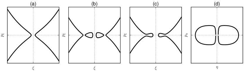
Figure 1: Representative phase plots in the three-dimensional case. The evolution of $\xi$ and $p_{\xi}$ (a,b,c) can be bound or unbound, depending on the initial conditions and on the values of the parameters of the system. By contrast, the evolution of $\eta$ and $p_{\eta}$ is always bound (d).

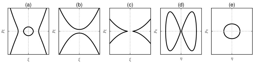
Figure 2: Representative phase plots in the bidimensional case. Similarly to the three-dimensional case, the evolution of $\xi$ and $p_{\xi}$ (a,b,c) can be bound or unbound, whereas the evolution of $\eta$ and $p_{\eta}$ is always bound (d,e).

We proceed now to determine the explicit solutions for $\xi\left(\tau\right)$ and $\eta\left(\tau\right)$ in the three-dimensional case. We will focus on the study of the solution for $\xi$, as the solution for $\eta$ differs only by notation. We will then use $\xi\left(\tau\right)$ and $\eta\left(\tau\right)$ to determine the solution for $\phi\left(\tau\right)$.

3 Solution by quadrature

The integration of eq. (27) yields

$$\int_{0}^{\tau}du=\pm\int_{\xi_{0}}^{\xi}\frac{udu}{\sqrt{\varepsilon u^{6}+2hu^{4}+2\alpha_{1}u^{2}-p_{\phi}^{2}}},$$ (30)

where the initial fictitious time has been set to zero, $u$ is a dummy integration variable and $\xi_{0}$ is the initial value of $\xi$. Before proceeding, we need to discuss briefly the nature of the sign ambiguity in this formula.

The left-hand side of eq. (30) represents the fictitious time needed by the dynamical system to evolve from the initial coordinate $\xi_{0}$ to an arbitrary coordinate $\xi$. As pointed out in the previous section, all phase plots are symmetric with respect to the horizontal axis, and thus, along a trajectory in phase space, each coordinate $\xi$ will be visited twice: once with a positive $p_{\xi}$ coordinate, and once with a negative $p_{\xi}$ coordinate. It follows that we can choose either sign in (30), and the left-hand side will then represent the evolution time along a portion of trajectory in which $p_{\xi}$ remains positive ($+$) or negative ($-$).

Changing now integration variable in the right-hand side of eq. (30) to

$$s=\frac{1}{2}u^{2},$$ (31)

we can rewrite the equation as

$$\tau =\pm\int_{\frac{1}{2}\xi_{0}^{2}}^{\frac{1}{2}\xi^{2}}\frac{ds}{\sqrt{8\varepsilon s^{3}+8hs^{2}+4\alpha_{1}s-p_{\phi}^{2}}}$$ (32)

$$=\pm\int_{\frac{1}{2}\xi_{0}^{2}}^{\frac{1}{2}\xi^{2}}\frac{ds}{\sqrt{f_{\xi}\left(s\right)}},$$ (33)

where $f_{\xi}\left(s\right)$ is a cubic polynomial in $s$. The integral in this expression is an elliptic integral, which can be computed and inverted to yield $\xi^{2}$ as function of $\tau$ using a formula by Weierstrass (see Whittaker & Watson, 1927, §20.6). After electing

$$f_{\xi}\left(s\right) =a_{4}+4a_{3}s+6a_{2}s^{2}+4a_{1}s^{3},$$ (34)

and defining

$$g_{2} =-4a_{1}a_{3}+3a_{2}^{2},$$ (35)

$$g_{3} =2a_{1}a_{2}a_{3}-a_{2}^{3}-a_{1}^{2}a_{4},$$ (36)

$$\wp_{\xi}\left(\tau\right) \equiv\wp\left(\tau;g_{2},g_{3}\right),$$ (37)

where $\wp\left(\tau;g_{2},g_{3}\right)$ is a Weierstrass elliptic function defined in terms of the invariants $g_{2}$ and $g_{3}$ (see Whittaker & Watson (1927), Chapter XX, and Abramowitz & Stegun (1964), Chapter 18), the evolution of $\xi^{2}$ in fictitious time is given by

$$\xi^{2} =\xi_{0}^{2}+\frac{1}{\left[\wp_{\xi}\left(\tau\right)-\frac{1}{24}f_{\xi}^{\prime\prime}\left(\frac{\xi_{0}^{2}}{2}\right)\right]^{2}}$$

$$\quad\cdot\left\{\frac{1}{2}f_{\xi}^{\prime}\left(\frac{\xi_{0}^{2}}{2}\right)\left[\wp_{\xi}\left(\tau\right)-\frac{1}{24}f_{\xi}^{\prime\prime}\left(\frac{\xi_{0}^{2}}{2}\right)\right]\vphantom{\sqrt{f_{\xi}\left(\frac{\xi_{0}^{2}}{2}\right)}}\right.$$

$$\quad\left.+\frac{1}{24}f_{\xi}\left(\frac{\xi_{0}^{2}}{2}\right)f_{\xi}^{\prime\prime\prime}\left(\frac{\xi_{0}^{2}}{2}\right)\pm\sqrt{f_{\xi}\left(\frac{\xi_{0}^{2}}{2}\right)}\wp_{\xi}^{\prime}\left(\tau\right)\right\}.$$ (38)

Here the $\pm$ sign represents the sign ambiguity discussed earlier, and the derivatives of $f_{\xi}$ are calculated with respect to the polynomial variable, while the derivative $\wp_{\xi}^{\prime}$ is calculated with respect to $\tau$. $\wp_{\xi}^{\prime}$ is related to $\wp$ via the relation

$$\left[\wp_{\xi}^{\prime}\left(z\right)\right]^{2}=4\wp_{\xi}^{3}\left(z\right)-g_{2}\wp_{\xi}\left(z\right)-g_{3}$$ (39)

(Abramowitz & Stegun, 1964, eq. 18.1.6). If $\xi_{0}^{2}/2$ is chosen as a root $\xi_{r}^{2}/2$ of $f_{\xi}$, then $f_{\xi}\left(\xi_{r}^{2}/2\right)=0$ and eq. (38) simplifies to

$$\xi^{2}=\xi_{r}^{2}+\frac{1}{2}\frac{f_{\xi}^{\prime}\left(\frac{\xi_{r}^{2}}{2}\right)}{\wp_{\xi}\left(\tau-\tau_{\xi}\right)-\frac{1}{24}f_{\xi}^{\prime\prime}\left(\frac{\xi_{r}^{2}}{2}\right)},$$ (40)

where $\tau_{\xi}$ is the fictitious time for which $\xi$ assumes the value $\xi_{r}$. The analogous expressions for $\eta$ are

$$\eta^{2} =\eta_{0}^{2}+\frac{1}{\left[\wp_{\eta}\left(\tau\right)-\frac{1}{24}f_{\eta}^{\prime\prime}\left(\frac{\eta_{0}^{2}}{2}\right)\right]^{2}}$$

$$\quad\cdot\left\{\frac{1}{2}f_{\eta}^{\prime}\left(\frac{\eta_{0}^{2}}{2}\right)\left[\wp_{\eta}\left(\tau\right)-\frac{1}{24}f_{\eta}^{\prime\prime}\left(\frac{\eta_{0}^{2}}{2}\right)\right]\vphantom{\sqrt{f_{\eta}\left(\frac{\eta_{0}^{2}}{2}\right)}}\right.$$

$$\quad\left.+\frac{1}{24}f_{\eta}\left(\frac{\eta_{0}^{2}}{2}\right)f_{\eta}^{\prime\prime\prime}\left(\frac{\eta_{0}^{2}}{2}\right)\pm\sqrt{f_{\eta}\left(\frac{\eta_{0}^{2}}{2}\right)}\wp_{\eta}^{\prime}\left(\tau\right)\right\}$$ (41)

and

$$\eta^{2}=\eta_{r}^{2}+\frac{1}{2}\frac{f_{\eta}^{\prime}\left(\frac{\eta_{r}^{2}}{2}\right)}{\wp_{\eta}\left(\tau-\tau_{\eta}\right)-\frac{1}{24}f_{\eta}^{\prime\prime}\left(\frac{\eta_{r}^{2}}{2}\right)}.$$ (42)

The formulæ (38) and (41) represent a general and complete closed-form solution for the squares $\xi^{2}$ and $\eta^{2}$ of the parabolic coordinates $\xi$ and $\eta$. Since $\xi$ and $\eta$ are non-negative by definition, in order to recover the solution for $\xi$ and $\eta$ it will be enough to take the principal square root of $\xi^{2}$ and $\eta^{2}$. The cartesian positions and velocities can be reconstructed using eqs. (2)-(4), where the derivatives of the parabolic coordinates with respect to the real time can be computed by inverting eqs. (11)-(13) (and by keeping in mind that $p_{\xi}$ and $p_{\eta}$ can be calculated by differentiating eqs. (38) and (41) with respect to $\tau$ – see eqs. (27) and (28)).

For simplicity’s sake, notational convenience and further analysis, however, it is desirable to be able to use the simplified formulæ (40) and (42) whenever possible. To this end, we first note how, from the considerations presented in the previous section, the polynomials $f_{\xi}$ and $f_{\eta}$ will always have at least one positive real root, with the exception of the bidimensional case for $f_{\xi}$ with $\alpha_{1}>0$ (displayed in Figure 2 (b)). The roots $\xi_{r}$ and $\eta_{r}$ of the cubic polynomials $f_{\xi}$ and $f_{\eta}$ can be computed exactly using the general formulæ for the roots of a cubic function. Secondly, in order to determine $\tau_{\xi}$ (and, analogously, $\tau_{\eta}$) we can use eq. (32) to write:

$$\tau_{\xi}=\pm\int_{\frac{1}{2}\xi_{0}^{2}}^{\frac{1}{2}\xi_{r}^{2}}\frac{ds}{\sqrt{8\varepsilon s^{3}+8hs^{2}+4\alpha_{1}s-p_{\phi}^{2}}}.$$ (43)

Following then Byrd (1971, eqs. (A7)–(A13)), we introduce the Tschirnhaus transformation (Cayley, 1861)

$$s=\sqrt[3]{\frac{1}{2\varepsilon}}s_{1}-\frac{1}{3}\frac{h}{\varepsilon}$$ (44)

in order to reduce the polynomial $f_{\xi}$ to a depressed cubic:

$$\tau_{\xi}=\pm\sqrt[3]{\frac{1}{2\varepsilon}}\int_{\sqrt[3]{2\varepsilon}\left(\frac{1}{2}\xi_{0}^{2}+\frac{1}{3}\frac{h}{\varepsilon}\right)}^{\sqrt[3]{2\varepsilon}\left(\frac{1}{2}\xi_{r}^{2}+\frac{1}{3}\frac{h}{\varepsilon}\right)}\frac{ds_{1}}{\sqrt{4s_{1}^{3}-h_{2}s_{1}-h_{3}}},$$ (45)

where

$$h_{2} =\sqrt[3]{\frac{1}{2\varepsilon}}\left(\frac{8}{3}\frac{h^{2}}{\varepsilon}-4\alpha_{1}\right),$$ (46)

$$h_{3} =\frac{4}{3}\frac{\alpha_{1}h}{\varepsilon}-\frac{16}{27}\frac{h^{3}}{\varepsilon^{2}}+p_{\phi}^{2}.$$ (47)

The integral can now be split into two separate Weierstrass normal elliptic integrals of the first kind,

$$\tau_{\xi}=\pm\sqrt[3]{\frac{1}{2\varepsilon}}\left[\int_{\sqrt[3]{2\varepsilon}\left(\frac{1}{2}\xi_{0}^{2}+\frac{1}{3}\frac{h}{\varepsilon}\right)}^{\infty}\frac{ds_{1}}{\sqrt{4s_{1}^{3}-h_{2}s_{1}-h_{3}}}\right.\\ \left.-\int_{\sqrt[3]{2\varepsilon}\left(\frac{1}{2}\xi_{r}^{2}+\frac{1}{3}\frac{h}{\varepsilon}\right)}^{\infty}\frac{ds_{1}}{\sqrt{4s_{1}^{3}-h_{2}s_{1}-h_{3}}}\right],$$ (48)

and solved in terms of the inverse Weierstrass elliptic function $\wp^{-1}$ as

$$\tau_{\xi}=\pm\sqrt[3]{\frac{1}{2\varepsilon}}\left\{\wp^{-1}\left[\sqrt[3]{2\varepsilon}\left(\frac{1}{2}\xi_{0}^{2}+\frac{1}{3}\frac{h}{\varepsilon}\right);h_{2},h_{3}\right]\right.\\ \left.-\wp^{-1}\left[\sqrt[3]{2\varepsilon}\left(\frac{1}{2}\xi_{r}^{2}+\frac{1}{3}\frac{h}{\varepsilon}\right);h_{2},h_{3}\right]\right\}.$$ (49)

The corresponding formula for $\tau_{\eta}$ can be obtained by switching $\varepsilon$ to $-\varepsilon$ and $\alpha_{1}$ to $\alpha_{2}$. It must be noted though that in this formula there are ambiguities regarding the computation of the inverse Weierstrass elliptic function, as $\wp^{-1}\left(z\right)$ is a multivalued function. The values of $\wp^{-1}$ in eq. (49) have then to be chosen appropriately in order to yield the correct result (as explained, e.g., in Hoggatt, 1955). As an alternative, it is possible to compute directly the integral in eq. (43) in terms of Legendre elliptic integrals using known formulæ (e.g., Gradshteĭn & Ryzhik, 2007, §3.131 and §3.138).

The solution for the third coordinate $\phi$ can now be computed directly by integrating eq. (29) with respect to $\tau$:

$$\int_{\phi_{0}}^{\phi}du=p_{\phi}\left[\int_{0}^{\tau}\frac{du}{\xi^{2}\left(u\right)}+\int_{0}^{\tau}\frac{du}{\eta^{2}\left(u\right)}\right].$$ (50)

It is easier to tackle the calculation via the simplified formulæ (40) and (42). The integrals on the right-hand side of eq. (50) are then in a form which can be solved through a formula involving $\wp^{\prime}$, $\wp^{-1}$ and the Weierstrass $\sigma$ and $\zeta$ functions (see Tannery & Molk (1893), chapter CXII, and Gradshteĭn & Ryzhik (2007), §5.141.5):

$$\int\frac{\wp\left(u\right)+\beta}{\gamma\wp\left(u\right)+\delta}du=\frac{u}{\gamma}+\frac{\delta-\beta\gamma}{\gamma^{2}\wp^{\prime}\left(v\right)}\left[\ln\frac{\sigma\left(u+v\right)}{\sigma\left(u-v\right)}-2u\zeta\left(v\right)\right],$$ (51)

where $v=\wp^{-1}\left(-\delta/\gamma\right)$. In this case, the multivalued character of $\wp^{-1}$ does not matter: it can be verified via the reduction formulæ of the Weierstrassian functions (Abramowitz & Stegun, 1964, §18.2) that any value of $v$ such that $\wp\left(v\right)=-\delta/\gamma$ will yield the same result in the right-hand side of eq. (51). The final result for $\phi$ is then:

$$\phi=\phi_{0}+2p_{\phi}\left\{\tau\left(\frac{1}{\gamma_{\xi}}+\frac{1}{\gamma_{\eta}}\right)+\frac{\delta_{\xi}-\beta_{\xi}\gamma_{\xi}}{\gamma_{\xi}^{2}\wp_{\xi}^{\prime}\left(u_{\xi}\right)}\right.\\ \cdot\left[\ln\frac{\sigma_{\xi}\left(\tau-\tau_{\xi}+u_{\xi}\right)}{\sigma_{\xi}\left(\tau-\tau_{\xi}-u_{\xi}\right)}-\ln\frac{\sigma_{\xi}\left(-\tau_{\xi}+u_{\xi}\right)}{\sigma_{\xi}\left(-\tau_{\xi}-u_{\xi}\right)}-2\tau\zeta_{\xi}\left(u_{\xi}\right)\right]\\ +\frac{\delta_{\eta}-\beta_{\eta}\gamma_{\eta}}{\gamma_{\eta}^{2}\wp_{\eta}^{\prime}\left(u_{\eta}\right)}\\ \left.\cdot\left[\ln\frac{\sigma_{\eta}\left(\tau-\tau_{\eta}+u_{\eta}\right)}{\sigma_{\eta}\left(\tau-\tau_{\eta}-u_{\eta}\right)}-\ln\frac{\sigma_{\eta}\left(-\tau_{\eta}+u_{\eta}\right)}{\sigma_{\eta}\left(-\tau_{\eta}-u_{\eta}\right)}-2\tau\zeta_{\eta}\left(u_{\eta}\right)\right]\vphantom{\frac{\tau}{\gamma_{\xi}}+\frac{\delta_{\xi}-\beta_{\xi}\gamma_{\xi}}{\gamma_{\xi}^{2}\wp_{\xi}^{\prime}\left(u_{\xi}\right)}}\right\},$$ (52)

where the following constants have been defined for notational convenience:

$$\beta_{\xi} =-\frac{1}{24}f_{\xi}^{\prime\prime}\left(\frac{\xi_{r}^{2}}{2}\right), \beta_{\eta} =-\frac{1}{24}f_{\eta}^{\prime\prime}\left(\frac{\eta_{r}^{2}}{2}\right),$$ (53)

$$\gamma_{\xi} =2\xi_{r}^{2}, \gamma_{\eta} =2\eta_{r}^{2},$$ (54)

$$\delta_{\xi} =f_{\xi}^{\prime}\left(\frac{\xi_{r}^{2}}{2}\right)+2\xi_{r}^{2}\beta_{\xi}, \delta_{\eta} =f_{\eta}^{\prime}\left(\frac{\eta_{r}^{2}}{2}\right)+2\eta_{r}^{2}\beta_{\eta},$$ (55)

$$u_{\xi} =\wp_{\xi}^{-1}\left(-\frac{\delta_{\xi}}{\gamma_{\xi}}\right), u_{\eta} =\wp_{\eta}^{-1}\left(-\frac{\delta_{\eta}}{\gamma_{\eta}}\right).$$ (56)

Starting from eq. (52), we adopt the subscript notation $\sigma_{\xi}$ and $\zeta_{\xi}$ to indicate Weierstrass $\sigma$ and $\zeta$ functions defined in terms of the same invariants as $\wp_{\xi}$.

4 The time equation

The final step in the solution of the Stark problem is to establish an explicit connection between real and fictitious time. To this end, we need to integrate eq. (16):

$$dt=\left[\xi^{2}\left(\tau\right)+\eta^{2}\left(\tau\right)\right]d\tau.$$ (57)

In the general case, according to eqs. (38) and (41), the exact solutions for $\xi^{2}\left(\tau\right)$ and $\eta^{2}\left(\tau\right)$ are of the form

$$A+B\wp^{\prime}\left(\tau\right),$$ (58)

where A and B are rational functions of $\wp\left(\tau\right)$. Then, according to the theory of elliptic functions, the antiderivative of (58) can be calculated in terms of $\wp$, $\wp^{\prime}$, $\wp^{-1}$ and the Weierstrass $\sigma$ and $\zeta$ functions. The integration method, due to Halphen (1886, chapter VII) (and explained in detail in Greenhill (1959, chapter VII)), involves the decomposition of $A$ and $B$ into separate fractions, resulting in the split of the integral into fundamental forms that can be integrated using the Weierstrassian functions.

It is again easier to use the simplified solutions (40) and (42), and thus obtain the time equation

$$t =\int_{0}^{\tau}\left[\xi^{2}\left(u\right)+\eta^{2}\left(u\right)\right]du$$ (59)

$$=\left(\xi_{r}^{2}+\eta_{r}^{2}\right)\tau+\frac{1}{2}\int_{0}^{\tau}\frac{f_{\xi}^{\prime}\left(\frac{\xi_{r}^{2}}{2}\right)}{\wp_{\xi}\left(u-\tau_{\xi}\right)-\frac{1}{24}f_{\xi}^{\prime\prime}\left(\frac{\xi_{r}^{2}}{2}\right)}du$$

$$\quad+\frac{1}{2}\int_{0}^{\tau}\frac{f_{\eta}^{\prime}\left(\frac{\eta_{r}^{2}}{2}\right)}{\wp_{\eta}\left(u-\tau_{\eta}\right)-\frac{1}{24}f_{\eta}^{\prime\prime}\left(\frac{\eta_{r}^{2}}{2}\right)}du.$$ (60)

The integrals appearing in eq. (60) are known and they can be computed directly. To this end, it would be tempting to apply the formulæ in Gradshteĭn & Ryzhik (2007, §5.141). However, as it can be verified by direct substitution using the exact solution of the cubic equation, $\frac{1}{24}f_{\xi}^{\prime\prime}\left(\frac{\xi_{r}^{2}}{2}\right)$ and $\frac{1}{24}f_{\eta}^{\prime\prime}\left(\frac{\eta_{r}^{2}}{2}\right)$ are always roots of the characteristic cubic equations

$$4t^{3}-g_{2}t-g_{3}=0,$$ (61)

associated to $\wp_{\xi}$ and $\wp_{\eta}$. Consequently, the formulæ in Gradshteĭn & Ryzhik (2007, §5.141) will be singular, and we have to use instead the results in Tannery & Molk (1893, §CXII), which yield the formula

$$\int\frac{du}{\wp\left(u\right)-e_{i}}=\frac{1}{g_{2}/4-3e_{i}^{2}}\left[ue_{i}+\zeta\left(u-\omega_{i}\right)\right].$$ (62)

In this formula, the $e_{i}$ represents the three roots of the characteristic cubic equation, while the $\omega_{i}$ are defined by the relation $e_{i}=\wp\left(\omega_{i}\right)$ (so that, following Abramowitz & Stegun (1964, eq. 18.3.1), two of the $\omega_{i}$ are the fundamental half-periods of $\wp$ and the third one is the sum of the fundamental half-periods). The solution of eq. (60) is thus:

$$t=\left(\xi_{r}^{2}+\eta_{r}^{2}\right)\tau+\frac{1}{2}\frac{f_{\xi}^{\prime}\left(\frac{\xi_{r}^{2}}{2}\right)}{g_{2,\xi}/4-3e_{i,\xi}^{2}}\cdot\\ \left[\tau e_{i,\xi}+\zeta_{\xi}\left(\tau-\tau_{\xi}-\omega_{i,\xi}\right)-\zeta_{\xi}\left(-\tau_{\xi}-\omega_{i,\xi}\right)\right]+\\ \frac{1}{2}\frac{f_{\eta}^{\prime}\left(\frac{\eta_{r}^{2}}{2}\right)}{g_{2,\eta}/4-3e_{i,\eta}^{2}}\cdot\\ \left[\tau e_{i,\eta}+\zeta_{\eta}\left(\tau-\tau_{\eta}-\omega_{i,\eta}\right)-\zeta_{\eta}\left(-\tau_{\eta}-\omega_{i,\eta}\right)\right].$$ (63)

This equation can be considered as the equivalent of Kepler’s equation for the Stark problem. Similarly to the two-body problem, it is constituted of a linear part modulated by two quasi-periodic transcendental parts (with the Weierstrass $\zeta$ function replacing the sine function appearing in Kepler’s equation). In this sense, the fictitious time $\tau$ can be regarded as a kind of eccentric anomaly for the Stark problem. According to eq. (16), the time equation is a monotonic function and its inversion can thus be achieved numerically using standard techniques (Newton-Raphson, bisection, etc.).

5 Analysis of the results

After having determined the full formal solution of the Stark problem in the previous sections, we now turn our attention to the interpretation of the results.

Before proceeding, we first need to point out how our solution to the Stark problem, as developed in the previous sections, is directly applicable to the three-dimensional case, but not in general to all bidimensional cases. As explained in §2.1, in certain bidimensional cases (specifically, when the constant of motion $\alpha_{1}$ is positive) the polynomial $p_{\xi}\left(\xi\right)$ might have no real zeroes, and thus the simplified formula (40) cannot be used. While in this case it is still possible to proceed to a complete solution via the full formula (38) in conjunction with the general theory for the integration of rational functions of elliptic functions (see Halphen (1886, chapter VII) and Greenhill (1959, chapter VII)), the resulting expressions for $\phi\left(\tau\right)$ and $t\left(\tau\right)$ will be more complicated than the formulæ obtained for the three-dimensional case.

An additional complication in the bidimensional case is the presence of the discontinuity discussed in §2.1. In correspondence of a polar transit, either $p_{\xi}$ or $p_{\eta}$ will switch sign. This discontinuity must be taken into account in the computation and inversion of the integral (32), and ultimately it has the effect of introducing a branching in the solutions for $\xi\left(\tau\right)$ and $\eta\left(\tau\right)$.

5.1 Quasi-periodicity and periodicity

Our solution to the Stark problem is based on the Weierstrass elliptic and related functions. Without giving a full account of the theory of the Weierstrassian functions (for which we refer to standard textbooks such as Whittaker & Watson (1927)), we will recall here briefly a few fundamental notions. To this end, we will employ the notation of Abramowitz & Stegun (1964, chapter 18).

The elliptic function $\wp\left(z;g_{2},g_{3}\right)$ is a doubly-periodic complex-valued function of a complex variable $z$ defined in terms of two complex parameters $g_{2}$ and $g_{3}$, called invariants. The complex primitive half-periods $\omega$ and $\omega^{\prime}$ of $\wp$ can be related to the invariants via formulæ involving elliptic integrals and the roots $e_{1}$, $e_{2}$ and $e_{3}$ of the characteristic cubic equation

$$4t^{3}-g_{2}t-g_{3}=0$$ (64)

(e.g., see Abramowitz & Stegun, 1964, §18.9). The sign of the modular discriminant

$$\Delta=g_{2}^{3}-27g_{3}^{2}$$ (65)

determines the nature of the roots $e_{1}$, $e_{2}$ and $e_{3}$. In the case of the Stark problem, the invariants are by definition real (see eqs. (35)–(36)), and thus the $(\omega,\omega^{\prime})$ pairs can be chosen as (real, imaginary) or complex conjugate (depending on the sign of $\Delta$). It is known from the theory of elliptic functions that there actually exist infinite pairs of fundamental half-periods for $\wp$, related to each other via integral linear combinations with unitary determinant (Hancock, 1910, §79). We can then always introduce two new half-periods $\omega_{R}$ (the real period) and $\omega_{C}$ (the complex period) such that $\omega_{R}$ is real and positive, and $\omega_{C}$ complex with positive imaginary part. The relation with the fundamental half-periods $\omega$ and $\omega^{\prime}$ from Abramowitz & Stegun (1964) is

$$\omega_{R} =\omega+\delta\omega^{\prime},$$ (66)

$$\omega_{C} =\omega^{\prime},$$ (67)

where $\delta=0$ if $\Delta>0$ and $\delta=1$ if $\Delta<0$. Since we are interested in the behaviour of $\wp$ on the real axis (as $\tau$ is a real-valued variable), we can then regard $\wp\left(\tau;g_{2},g_{3}\right)$ as a singly-periodic real-valued function of period $2\omega_{R}$.

It follows then straightforwardly from eqs. (38)–(42) that $\xi\left(\tau\right)$ and $\eta\left(\tau\right)$ are both periodic in $\tau$ with periods that, in general, will be different. Conversely, from eq. (52), it follows immediately that $\phi\left(\tau\right)$ is not periodic. Indeed, $\phi\left(\tau\right)$ is a function of the form

$$f\left(\tau\right)=A+B\tau+C_{\xi}\ln\frac{\sigma_{\xi}\left(\tau+a_{\xi}\right)}{\sigma_{\xi}\left(\tau+b_{\xi}\right)}+C_{\eta}\ln\frac{\sigma_{\eta}\left(\tau+a_{\eta}\right)}{\sigma_{\eta}\left(\tau+b_{\eta}\right)},$$ (68)

where $A$, $B$, $C$, $a$ and $b$ are constants. It is now interesting to note that, according to eqs. (16) and (29), if $\xi$ and $\eta$ have real half-periods $\omega_{R,\xi}$ and $\omega_{R,\eta}$ such that

$$\frac{\omega_{R,\xi}}{\omega_{R,\eta}}=\frac{n}{m},$$ (69)

with $n$ and $m$ coprime natural numbers (or, in other words, $\omega_{R,\xi}$ and $\omega_{R,\eta}$ are commensurable), then $d\phi/d\tau$ becomes a periodic function with period $T=2m\omega_{R,\xi}=2n\omega_{R,\eta}$. Recalling the quasi-periodicity of $\sigma$ via the relation (Abramowitz & Stegun, 1964, eq. 18.2.20)

$$\sigma\left(z+2M\omega+2N\omega^{\prime}\right)=\left(-1\right)^{M+N+MN}\sigma\left(z\right)\cdot\\ \mathrm{e}^{\left(z+M\omega+N\omega^{\prime}\right)\left[2M\zeta\left(\omega\right)+2N\zeta\left(\omega^{\prime}\right)\right]},$$ (70)

with $M,N\in\mathbb{Z}$, we can then write for eq. (68)

$$f\left(\tau+T\right)=A+B\tau+C_{\xi}\ln\frac{\sigma_{\xi}\left(\tau+a_{\xi}\right)}{\sigma_{\xi}\left(\tau+b_{\xi}\right)}+C_{\eta}\ln\frac{\sigma_{\eta}\left(\tau+a_{\eta}\right)}{\sigma_{\eta}\left(\tau+b_{\eta}\right)}\\ +BT+2mC_{\xi}\left(a_{\xi}-b_{\xi}\right)\zeta_{\xi}\left(\omega_{R,\xi}\right)\\ +2nC_{\eta}\left(a_{\eta}-b_{\eta}\right)\zeta_{\eta}\left(\omega_{R,\eta}\right),$$ (71)

or, more succinctly,

$$f\left(\tau+T\right)=f\left(\tau\right)+D,$$ (72)

where $D$ is the constant

$$D=BT+2mC_{\xi}\left(a_{\xi}-b_{\xi}\right)\zeta_{\xi}\left(\omega_{R,\xi}\right)\\ +2nC_{\eta}\left(a_{\eta}-b_{\eta}\right)\zeta_{\eta}\left(\omega_{R,\eta}\right).$$ (73)

Thus, if $\xi\left(\tau\right)$ and $\eta\left(\tau\right)$ have commensurable periods, $\phi\left(\tau\right)$ is an arithmetic quasi-periodic function of $\tau$. The geometric meaning of this quasi-periodicity is that, after a quasi-period $T$, the test particle will be in a position that results from a rotation around the $z$ axis of the original position. The particle’s trajectory will thus draw a rotationally-symmetric figure in space.

Quasi-periodic orbits can be found via a numerical search for a set of initial conditions and constant acceleration field $\varepsilon$ that satisfies the commensurability relation on the periods of $\xi$ and $\eta$. The numerical search can be setup as the minimisation of the function $\left(m\omega_{R,\xi}-n\omega_{R,\eta}\right)^{2}$ for two chosen coprime integers $n$ and $m$. A representative quasi-periodic orbit found this way using the PaGMO optimiser (Biscani et al., 2010) is displayed in Figure 3.

Periodic orbits can also be found in a similar way by imposing the additional condition $p\phi(T)=2\pi$, where $p\in\mathbb{Z}$. For any triplet of $\left(n,m,p\right)$ integers, one has then to solve numerically an optimisation problem that yields periodic orbits such as the one displayed in Figure 4 for a case $n=1$, $m=2$, and $p=7$.

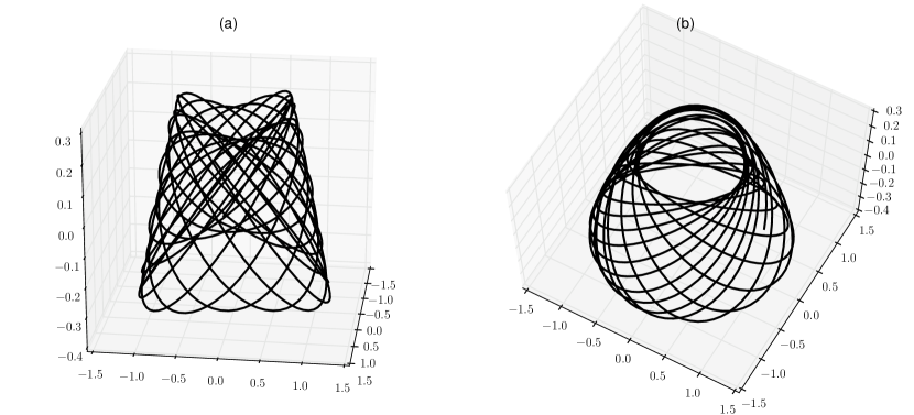
Figure 3: Three-dimensional plots of a representative quasi-periodic orbit, seen from the side (a) and from the top (b). In this specific case, the periods of $\xi$ and $\eta$ in fictitious time are in a ratio of $6/5$ within an accuracy of $\sim 10^{-11}$.

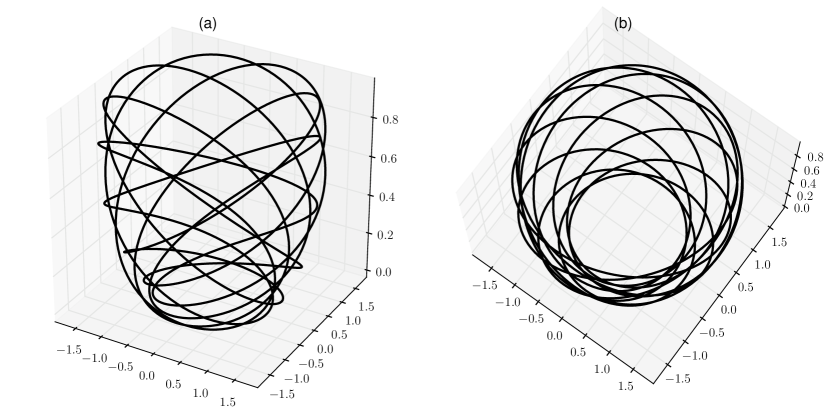
Figure 4: Three-dimensional plots of a representative periodic orbit ($n=1$, $m=2$, $p=7$), seen from the side (a) and from the top (b). One period of the trajectory is displayed. In this specific case, the trajectory is closed at the end of one period with an accuracy of $\sim 10^{-5}$.

5.2 Bound and unbound orbits

The solution of the Stark problem in terms of the Weierstrassian functions allows to determine the conditions under which the motion is bound. As we have seen in the previous sections, the parabolic coordinate $\eta$ is always bound, whereas $\xi$ can be either bound or unbound. From the general solution (38), it is easily deduced that the formula for $\xi\left(\tau\right)$ has a pole (and thus $\xi$ is unbound) when the denominator is zero, i.e., under the condition

$$\wp_{\xi}\left(\tau\right)-\frac{1}{24}f_{\xi}^{\prime\prime}\left(\frac{\xi_{0}^{2}}{2}\right)=0.$$ (74)

Recalling now that $\wp_{\xi}\left(\tau\right)$ is analytical everywhere except at the poles (where it behaves like $1/\tau^{2}$ around $\tau=0$), it can be deduced from the properties of parity and periodicity that $\wp_{\xi}\left(\tau\right)$ must have a global minimum within the real period $2\omega_{R}$. Moreover, since $\wp_{\xi}$ satisfies the differential equation (39), the condition for the existence of a stationary point is

$$\wp_{\xi}\left(\tau\right)=e_{i},$$ (75)

where $e_{i}$ represents the roots of the cubic equation (64). It is known (Abramowitz & Stegun, 1964, eq. 18.3.1) that $\wp_{\xi}\left(\omega_{i}\right)=e_{i}$, where

$$\omega_{1} =\omega,$$ (76)

$$\omega_{2} =\omega+\omega^{\prime},$$ (77)

$$\omega_{3} =\omega^{\prime},$$ (78)

which implies that the global minimum of $\wp_{\xi}\left(\tau\right)$ is in correspondence of $\tau=\omega_{R}$. We can then conclude that the condition for bound motion is

$$e_{R}>\frac{1}{24}f_{\xi}^{\prime\prime}\left(\frac{\xi_{0}^{2}}{2}\right),$$ (79)

where we have denoted with $e_{R}$ the root of the cubic equation (64) for which $\wp_{\xi}\left(\omega_{R}\right)=e_{R}$. Figure 5 displays the evolution of two representative bound orbits in the three-dimensional space.

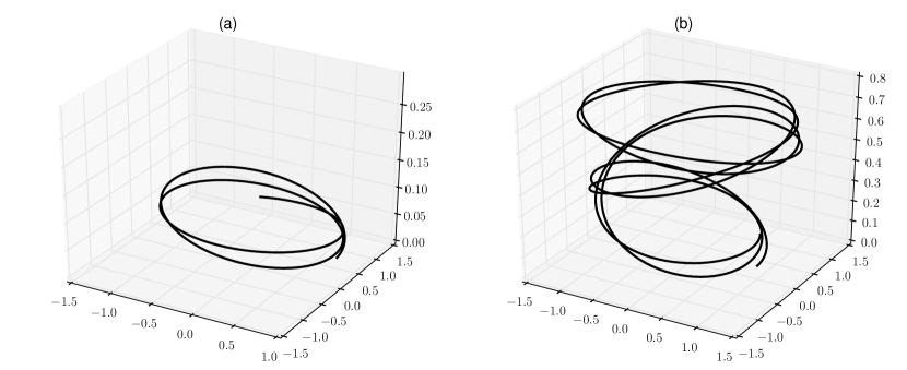
Figure 5: Three-dimensional plots of two representative bound orbits sharing the same initial conditions but with different values for the constant acceleration field. The initial condition corresponds (in absence of the external acceleration field) to a quasi-circular Keplerian orbit lying close to the $xy$ plane. The acceleration field is weaker in (a), whereas in (b) it is close to the critical value for which the orbit becomes unbound.

Figure 6 displays the evolution in $\tau$ of the parabolic coordinates and of the real time $t$ in a bound and an unbound case. It is interesting to note that in the unbound case only $\xi$ and $t$ present vertical asymptotes, whereas $\eta$ and $\phi$ assume finite values when $\xi$ and $t$ go to infinity. With respect to the evolution in real time $t$, this means that $\eta$ and $\phi$ tend asymptotically to finite values for $t\to\infty$. At infinity, the trajectory of the test particle is determined solely by the constant acceleration field and will thus be a parabola. The plane in which such asymptotic parabola lies is perpendicular to the $xy$ plane and its orientation is determined by the value to which the azimuthal angle $\phi$ tends asymptotically (which can be determined exactly by calculating the value of $\phi$ at the end of one period in fictitious time). This result could prove to be particularly useful in the design of powered planetary kicks (or flybys), a technique vastly used in modern interplanetary trajectory design (Danby, 1988). Planetary kicks are traditionally designed assuming an unperturbed hyperbolic motion around a certain planet. The outgoing conditions are then simply determined by the analytical expression governing Keplerian motion (i.e., a rotation of the hyperbolic access velocity). A different type of powered flyby can be considered, in which the spacecraft thrusts continuously in a fixed inertial direction. In such a case, and ignoring the fuel mass loss, the spacecraft conditions at infinity (i.e., when leaving the planet’s sphere of influence) can be determined exactly by a fully-analytical solution such as the one presented here.

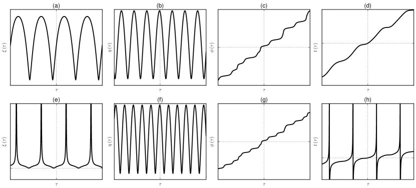
Figure 6: Representative plots of the evolution in fictitious time $\tau$ of the parabolic coordinates $\xi$, $\eta$ and $\phi$ and of the real time $t$ in a bound ((a)-(d), first row) and an unbound ((e)-(h), second row) orbit. In the unbound case, the $\xi$ coordinate (e) and the real time $t$ (h) reach infinity in a finite amount of fictitious time.

5.3 Equilibrium points and displaced circular orbits

We turn now our attention to the analysis of the equilibrium points of the Stark problem. It is useful to consider initially the Hamiltonian in cartesian coordinates and real time $t$ resulting from the Lagrangian (1). The equations of motion are, trivially,

$$\frac{dx}{dt} =v_{x}, \frac{dv_{x}}{dt} =-\frac{\mu x}{r^{3}},$$ (80)

$$\frac{dy}{dt} =v_{y}, \frac{dv_{y}}{dt} =-\frac{\mu y}{r^{3}},$$ (81)

$$\frac{dz}{dt} =v_{z}, \frac{dv_{z}}{dt} =-\frac{\mu z}{r^{3}}+\varepsilon.$$ (82)

The only equilibrium point for this system is for $v_{x}=v_{y}=v_{z}=x=y=0$ and $z=\sqrt{\mu/\varepsilon}$. That is, the test particle is stationary on the positive $z$ axis at a distance from the origin such that the Newtonian attraction and the external acceleration field counterbalance each other. We refer to this unstable critical point as the cartesian stationary equilibrium.

Back in parabolic coordinates and fictitious time $\tau$, a first straightforward observation is that the cartesian stationary equilibrium cannot be handled in this coordinate system, as it corresponds to a position in which the azimuthal angle $\phi$ is undefined. Secondly, since $d\phi/d\tau$ is a monotonic function according to (29), it follows that there cannot be a parabolic stationary equilibrium point, and that only the coordinates $\xi$ and $\eta$ can be in a stationary point. From the definition (5) we can deduce how a trajectory in which $\xi$ is constant is constrained to a circular paraboloid symmetric with respect to the $z$ axis and defined by the equation

$$z=\frac{\xi_{0}^{4}-x^{2}-y^{2}}{2\xi_{0}^{2}},$$ (83)

resulting from the inversion of eq. (5). Similarly, a trajectory with constant $\eta$ will be constrained to the paraboloid defined by

$$z=\frac{x^{2}+y^{2}-\eta_{0}^{4}}{2\eta_{0}^{2}}$$ (84)

(via inversion of eq. (6)).

It is then interesting to note how a trajectory in which both $\xi$ and $\eta$ are constant will be constrained to the intersection of two coaxial circular paraboloids with opposite orientation. That is, the trajectory will follow a circle centred on the $z$ axis and parallel to the $xy$ plane. Additionally, according to eqs. (16) and (29), such a circular trajectory will have constant angular velocity both in fictitious and real time. Such orbits are known in the literature as static orbits (Forward, 1991), displaced circular orbits (Dankowicz, 1994; Lantoine & Russell, 2011), displaced non-Keplerian orbits (McInnes, 1998), or sombrero orbits (Namouni & Guzzo, 2007).

From a physical point of view, displaced circular orbits are possible when the initial conditions satisfy the following requirements:

• the distance from the $xy$ plane is such that the net force acting on the test particle is perpendicular to the $z$ axis (i.e., the total force has zero $z$ component),

• the initial velocity vector is lying on the plane $\Pi$ of the displaced circular orbit, it is perpendicular to the projection of the position vector on $\Pi$ and its magnitude has the same value it would assume in a circular Keplerian orbit with a fictitious central body lying in correspondence of the $z$ axis on the $\Pi$ plane (where the mass of the fictitious body is generating the total force experienced by the test particle).

In other words, with these initial conditions the test particle evolves along a Keplerian planar circular orbit under the influence of a fictitious body lying on the positive $z$ axis. These requirements are satisfied by the following cartesian initial conditions:

$$\bm{r}_{0} =\left(\sqrt{\left(\frac{z\mu}{\varepsilon}\right)^{\frac{2}{3}}-z^{2}},0,z\right),$$ (85)

$$\bm{v}_{0} =\left(0,\sqrt{\frac{\varepsilon}{z}\left[\left(\frac{z\mu}{\varepsilon}\right)^{\frac{2}{3}}-z^{2}\right]},0\right),$$ (86)

where $z>0$ and where we have taken advantage of the cylindrical symmetry of the problem by choosing, without loss of generality, a set of initial conditions on the $xz$ plane. It is clear from eqs. (85) and (86) that there exist a limit on the value of $z$ after which displaced circular orbits are not possible because the radicand in the expression for the $x$ coordinate becomes negative. Physically, this means that the gravitational force cannot counterbalance the constant acceleration field in the $z$ direction. This limit value is clearly in correspondence of the cartesian stationary equilibrium.

From a mathematical point of view, a displaced circular orbit must turn the solutions $\xi\left(\tau\right)$ and $\eta\left(\tau\right)$ into constants. From eqs. (40) and (42) it is clear that these expressions can become constants only when $f_{\xi}^{\prime}\left(\frac{\xi_{r}^{2}}{2}\right)$ and $f_{\eta}^{\prime}\left(\frac{\eta_{r}^{2}}{2}\right)$ are zero. This condition is equivalent to the requirement that the two polynomials $f_{\xi}$ and $f_{\eta}$ have roots of multiplicity greater than one. From the point of view of the theory of dynamical systems, the two polynomials need to have roots of multiplicity greater than one because otherwise the zeroes of the differential equations (27) and (28) are in correspondence of a point in which the equations lose their properties of differentiability and Lipschitz continuity, and the resulting equilibria are thus spurious.

It can be verified by direct substitution that the initial conditions (85) and (86), after the transformation into parabolic coordinates, are roots of both the characteristic polynomials $f_{\xi}$ and $f_{\eta}$ and of their derivatives. Our solution in terms of Weierstrassian functions is thus consistent with known results (e.g., see Namouni & Guzzo, 2007) regarding the existence and characterisation of the equilibrium points in the Stark problem.

6 Conclusions

In this paper we introduced a new solution to the Stark problem based on Weierstrass elliptic and related functions. Our treatment yields an exact (i.e., non-perturbative) and explicit solution of the full three-dimensional problem in terms of a set of unique formulæ valid for all initial conditions and physical parameters of the system. Formally, the result is remarkably similar to the solution of the two-body problem: the evolution of the coordinates is given as a function of an anomaly (or, a fictitious time) connected to the real time by a transcendental equation.

The simplicity of our formulation allows us to derive several new results. In particular, we were able to formulate conditions for the existence of quasi-periodic and periodic orbits, and to successfully identify instances of (quasi) periodic orbits using numerical techniques. We were also able to formulate a new simple analytical criterion to study the boundness of the motion, a result that can be particularly interesting for astrodynamical applications (e.g., in the study of the ejection of dust grains in the outer Solar System – see Belyaev & Rafikov (2010) and Pástor (2012)). Another result of astrodynamical interest (in connection to the design of powered flyby manoeuvres) is the identification of an analytical formula for the determination of the orientation of the asymptotic planes of motion at infinity in case of unbound orbits.

Our analysis shows how the Weierstrassian formalism can be fruitfully applied to yield a new insight in the dynamics of the Stark problem. We hope that our results will contribute to revive the interest in this beautiful and powerful mathematical tool.

Appendix A Implementation details

A.1 Implementation of the Weierstrassian functions

The Weierstrassian functions are not as readily available in scientific computation packages as other special functions. Following Abramowitz & Stegun (1964, §18.9 and §18.10), it is possible to express them in terms of Jacobi elliptic and theta functions. The recipes in Abramowitz & Stegun (1964) do not present particular difficulties in terms of implementation details. A minor complication is that the cases in which the Weierstrass invariant $g_{3}$ is negative are transformed in non-negative $g_{3}$ via the homogeneity relation

$$\wp\left(z;g_{2},g_{3}\right)=-\wp\left(\imath z;g_{2},-g_{3}\right)$$ (87)

(and similar relations hold for $\zeta$ and $\sigma$). This transformation is not problematic for the computation of the values of the functions, but it needs to be properly taken into account when computing auxiliary quantities such as the half-periods and the roots of the characteristic cubic equations.

Regarding the half-periods, it is seen from eq. (87) how the effect of the homogeneity relation is that of a rotation of the half-periods by $-\pi/2$ in the complex plane (via the $\imath$ factor applied to the argument $z$ on the right-hand side). The half-periods can then be first calculated in the transformed non-negative $g_{3}$ case, and afterwards they can be rotated back to obtain the original half-periods.

Regarding the roots of the characteristic polynomial

$$y=4x^{3}-g_{2}x-g_{3},$$ (88)

one can see how a change in sign in $g_{3}$ corresponds to a reflection with respect to both the $x$ and $y$ axes. The net effect will thus be equivalent to a simple change of the sign of all roots.

For the actual implementation of the Weierstrassian functions, we used the elliptic functions module of the multiprecision Python library mpmath (Johansson et al., 2011).

A.2 On the computation of the complex logarithms in equation (52)

The solution for the evolution of the $\phi$ coordinate in fictitious time, eq. (52), involves, in the general case, the computation of complex logarithms. Since the complex logarithm is a multivalued function, care must be taken in order to select values that yield physically meaningful solutions.

The standard way of proceeding when dealing with complex logarithms is to restrict the computation to the principal value $\operatorname{Log}$ of the logarithm, i.e., the unique value whose imaginary part lies in the interval $\left(-\pi,\pi\right]$. In doing so, if one takes the logarithm of a complex function whose values cross the negative real axis (i.e., the branch cut of $\operatorname{Log}$), a discontinuity will arise – the imaginary part of the logarithm of the function will jump from $\pi$ to $-\pi$ (or vice versa). In the case of the Stark problem, this means that $\phi\left(\tau\right)$ will be discontinuous. These discontinuities are merely an artefact of the way of choosing a particular logarithm value among all the possible ones, and they need to be dealt with in order to produce a physically correct (i.e., continuous) solution.

We start by recalling the following series expansion for the logarithm of $\sigma$ (Tannery & Molk, 1893, §CVI):

$$\operatorname{Log}\sigma\left(u\right)=\operatorname{Log}\frac{2\omega_{R}}{\pi}+\frac{\eta_{R}u^{2}}{2\omega_{R}}+\operatorname{Log}\sin\frac{\pi u}{2\omega_{R}}\\ +\sum_{r=1}^{\infty}\frac{q^{2r}}{r\left(1-q^{2r}\right)}\left(2\sin\frac{r\pi u}{2\omega_{R}}\right)^{2},$$ (89)

where $\eta_{R}=\zeta\left(\omega_{R}\right)$ and $q=\exp\left(\imath\pi\frac{\omega_{C}}{\omega_{R}}\right)$, and $u$ is decomposed into its components along the fundamental periods as

$$u=2\alpha\omega_{R}+2\beta\omega_{C},$$ (90)

with $\alpha,\beta\in\mathbb{R}$. This series expansion is convergent for $\left|\beta\right|<1$, or, in other words, as long as $u$ is confined to the strip in the complex plane defined by $\left|\Im\left(u\right)\right|<2\Im\left(\omega_{C}\right)$.

We turn now to the study of the behaviour of the series expansion (89) within the real period $2\omega_{R}$ and in the positive half of the strip of convergence. That is, we study the behaviour of the series expansion of $\operatorname{Log}\sigma\left[x_{\ast}+\imath 2\beta\Im\left(\omega_{C}\right)\right]$, with $x_{\ast}$ as a real variable in the interval $\left[0,2\omega_{R}\right)$ and $0<\beta<1$. We first note that, from eq. (89), there exists a potential discontinuity in the computation of the complex logarithm

$$\operatorname{Log}\sin\frac{\pi\left[x_{\ast}+\imath 2\beta\Im\left(\omega_{C}\right)\right]}{2\omega_{R}},$$ (91)

when its argument crosses the negative real axis. However, by applying elementary trigonometric identities, we can write

$$\Re\left\{\sin\frac{\pi\left[x_{\ast}+\imath 2\beta\Im\left(\omega_{C}\right)\right]}{2\omega_{R}}\right\} =\sin\frac{\pi x_{\ast}}{2\omega_{R}}\cosh\frac{\pi\beta\Im\left(\omega_{C}\right)}{\omega_{R}},$$ (92)

$$\Im\left\{\sin\frac{\pi\left[x_{\ast}+\imath 2\beta\Im\left(\omega_{C}\right)\right]}{2\omega_{R}}\right\} =\cos\frac{\pi x_{\ast}}{2\omega_{R}}\sinh\frac{\pi\beta\Im\left(\omega_{C}\right)}{\omega_{R}}.$$ (93)

That is, the argument of the logarithm in (91) crosses the real axis when $x_{\ast}=\omega_{R}$. But then, for $x_{\ast}=\omega_{R}$, the real part (92) of the argument of the logarithm is strictly positive (as the hyperbolic cosine is a strictly positive function), and hence the crossing of the real axis does not happen in correspondence of the branch cut of the principal value of the logarithm. This means that, for $x_{\ast}\in\left[0,2\omega_{R}\right)$, the series expansion (89) of $\operatorname{Log}\sigma\left[x_{\ast}+\imath 2\beta\Im\left(\omega_{C}\right)\right]$ is a continuous function.

Outside the interval $\left[0,2\omega_{R}\right)$, we can represent a variable $x\in\mathbb{R}$ as $x=x_{\ast}+2N\omega_{R}$, where $N\in\mathbb{Z}$. Recalling now the definition of the Weierstrass sigma function (Greenhill, 1959, §195), we can write

$$\sigma\left[x+\imath 2\beta\Im\left(\omega_{C}\right)\right]=\sigma\left[x_{\ast}+2N\omega_{R}+\imath 2\beta\Im\left(\omega_{C}\right)\right]\\ =\exp\left\{\operatorname{Log}\left[x_{\ast}+2N\omega_{R}+\imath 2\beta\Im\left(\omega_{C}\right)\right]+\vphantom{\int_{0}^{x_{\ast}+2N\omega_{R}+\imath 2\beta\Im\left(\omega_{C}\right)}\left[\zeta\left(z\right)-\frac{1}{z}\right]dz}\right.\\ \left.\int_{0}^{x_{\ast}+2N\omega_{R}+\imath 2\beta\Im\left(\omega_{C}\right)}\left[\zeta\left(z\right)-\frac{1}{z}\right]dz\right\}.$$ (94)

We can split the integral in eq. (94) as

$$\int_{0}^{x_{\ast}+2N\omega_{R}+\imath 2\beta\Im\left(\omega_{C}\right)}\left[\zeta\left(z\right)-\frac{1}{z}\right]dz\\ =\int_{0}^{x_{\ast}+\imath 2\beta\Im\left(\omega_{C}\right)}\left[\zeta\left(z\right)-\frac{1}{z}\right]dz\\ +\int_{x_{\ast}+\imath 2\beta\Im\left(\omega_{C}\right)}^{x_{\ast}+2N\omega_{R}+\imath 2\beta\Im\left(\omega_{C}\right)}\left[\zeta\left(z\right)-\frac{1}{z}\right]dz,$$ (95)

and, following (Tannery & Molk, 1893, §CXVII), the third integral in eq. (95) can be computed as

$$\int_{x_{\ast}+\imath 2\beta\Im\left(\omega_{C}\right)}^{x_{\ast}+2N\omega_{R}+\imath 2\beta\Im\left(\omega_{C}\right)}\left[\zeta\left(z\right)-\frac{1}{z}\right]dz\\ =\operatorname{Log}\left[x_{\ast}+\imath 2\beta\Im\left(\omega_{C}\right)\right]-\operatorname{Log}\left[x_{\ast}+2N\omega_{R}+\imath 2\beta\Im\left(\omega_{C}\right)\right]\\ +2N\eta_{R}\left[x_{\ast}+\imath 2\beta\Im\left(\omega_{C}\right)+N\omega_{R}\right]-\imath N\pi.$$ (96)

In other words,

$$\operatorname{Log}\sigma\left[x+\imath 2\beta\Im\left(\omega_{C}\right)\right]=\operatorname{Log}\sigma\left[x_{\ast}+\imath 2\beta\Im\left(\omega_{C}\right)\right]\\ +2N\eta_{R}\left[x_{\ast}+\imath 2\beta\Im\left(\omega_{C}\right)+N\omega_{R}\right]-\imath N\pi,$$ (97)

which corresponds to the homogeneity relation in Abramowitz & Stegun (1964, §18.2). Since, as we have seen, $\operatorname{Log}\sigma\left[x_{\ast}+\imath 2\beta\Im\left(\omega_{C}\right)\right]$ is a continuous function, the only possible discontinuities in eq. (97) are in the neighbourhood of $x=2N\omega_{R}$, where $x_{\ast}$ changes discontinuously by $\pm 2\omega_{R}$ and $N$ by $\pm 1$. For $x=2N\omega_{R}$, $x_{\ast}$ is zero and the limit from the right is

$$L^{+}=\lim_{x\to\left(2N\omega_{R}\right)^{+}}\operatorname{Log}\sigma\left[x+\imath 2\beta\Im\left(\omega_{C}\right)\right]\\ =\operatorname{Log}\sigma\left[\imath 2\beta\Im\left(\omega_{C}\right)\right]+2N\eta_{R}\left[\imath 2\beta\Im\left(\omega_{C}\right)+N\omega_{R}\right]-\imath N\pi.$$ (98)

The limit from the left instead is

$$L^{-}=\lim_{x\to\left(2N\omega_{R}\right)^{-}}\operatorname{Log}\sigma\left[x+\imath 2\beta\Im\left(\omega_{C}\right)\right]\\ =\operatorname{Log}\sigma\left[2\omega_{R}+\imath 2\beta\Im\left(\omega_{C}\right)\right]\\ +2\left(N-1\right)\eta_{R}\left[\imath 2\beta\Im\left(\omega_{C}\right)+\left(N+1\right)\omega_{R}\right]-\imath\left(N-1\right)\pi.$$ (99)

By using the series expansion (89), we can write

$$L^{+}=\operatorname{Log}\frac{2\omega_{R}}{\pi}+\frac{\eta_{R}\left[\imath 2\beta\Im\left(\omega_{C}\right)\right]^{2}}{2\omega_{R}}+\operatorname{Log}\sin\frac{\imath\pi\beta\Im\left(\omega_{C}\right)}{\omega_{R}}\\ +\sum_{r=1}^{\infty}\frac{q^{2r}}{r\left(1-q^{2r}\right)}\left\{2\sin\frac{r\pi\left[\imath 2\beta\Im\left(\omega_{C}\right)\right]}{2\omega_{R}}\right\}^{2}\\ +2N\eta_{R}\left[\imath 2\beta\Im\left(\omega_{C}\right)+N\omega_{R}\right]-\imath N\pi$$ (100)

and

$$L^{-}=\operatorname{Log}\frac{2\omega_{R}}{\pi}+\frac{\eta_{R}\left[2\omega_{R}+\imath 2\beta\Im\left(\omega_{C}\right)\right]^{2}}{2\omega_{R}}\\ +\operatorname{Log}\sin\frac{\pi\left[2\omega_{R}+\imath 2\beta\Im\left(\omega_{C}\right)\right]}{2\omega_{R}}\\ +\sum_{r=1}^{\infty}\frac{q^{2r}}{r\left(1-q^{2r}\right)}\left\{2\sin\frac{r\pi\left[2\omega_{R}+\imath 2\beta\Im\left(\omega_{C}\right)\right]}{2\omega_{R}}\right\}^{2}\\ +2\left(N-1\right)\eta_{R}\left[\imath 2\beta\Im\left(\omega_{C}\right)+\left(N+1\right)\omega_{R}\right]-\imath\left(N-1\right)\pi.$$ (101)

By noting that

$$\operatorname{Log}\left[\pm\sin\frac{\imath\pi\beta\Im\left(\omega_{C}\right)}{\omega_{R}}\right]=\operatorname{Log}\sinh\frac{\pi\beta\Im\left(\omega_{C}\right)}{\omega_{R}}\pm\imath\frac{\pi}{2}$$ (102)

(as $\beta$, $\Im\left(\omega_{C}\right)$ and $\omega_{R}$ are all real positive quantities by definition), it can be verified, after a few algebraic passages, that $L^{+}=L^{-}$, and thus the right-hand side of eq. (97) is a continuous function.

Going back to the Stark problem, we can immediately see how the logarithmic forms in eq. (52) are in the same form as in eq. (97). For instance, in

$$\ln\sigma_{\xi}\left(\tau-\tau_{\xi}+u_{\xi}\right)$$ (103)

the real variable is $\tau$, while $u_{\xi}$ is defined as

$$u_{\xi}=\wp_{\xi}^{-1}\left(-\frac{\delta_{\xi}}{\gamma_{\xi}}\right).$$ (104)

Since $u_{\xi}$ is the result of an inverse $\wp$, it can always be chosen inside the fundamental period parallelogram, where the condition of convergence of the series expansion (89) ($\left|\beta\right|<1$) is always satisfied. Eq. (97) can thus be substituted into eq. (52) to provide a formula for $\phi\left(\tau\right)$ free of discontinuities.

A.3 Solution algorithm

In this section, we are going to detail the steps of a possible implementation of our solution to the Stark problem, starting from initial conditions in cartesian coordinates. The algorithm outlined below requires the availability of an implementation of the Weierstrassian functions $\wp$, $\wp^{\prime}$, $\wp^{-1}$, $\zeta$ and $\sigma$, and of a few related ancillary functions (e.g., for the conversion of the invariants $g_{2}$ and $g_{3}$ to the half-periods $\omega$ and $\omega^{\prime}$). Chapter 18 in Abramowitz & Stegun (1964) details how to implement these requirements in terms of Jacobi theta and elliptic functions and integrals.

The algorithm is given as follows:

1. transform the initial cartesian coordinates into parabolic coordinates via eqs. (5)-(7), and compute the initial Hamiltonian momenta $p_{\xi}$, $p_{\eta}$ and $p_{\phi}$ via eqs. (11)-(13);

2. compute the constants of motion $h$, $\alpha_{1}$ and $\alpha_{2}$, through the substitution of the initial Hamiltonian coordinates and momenta into eqs. (15), (25) and (26);

3. calculate the roots of the bicubic polynomials on the right-hand sides of eqs. (27) and (28). Among the positive roots, choose one for each of the two polynomials as the $\xi_{r}$ and $\eta_{r}$ values. In the case of the $\xi$ coordinate, $\xi_{r}$ must be a reachable root, i.e., a value that will actually be assumed by $\xi$ at some point in time;

4. compute the fictitious times of “pericentre passage” $\tau_{\xi}$ and $\tau_{\eta}$ via eq. (43). The integral can be solved either via the inverse Weierstrass function (Hoggatt, 1955) or via elliptic integrals (e.g., Gradshteĭn & Ryzhik, 2007, §3.131 and §3.138). The signs of $\tau_{\xi}$ and $\tau_{\eta}$ must be chosen in accordance with the choice of $\xi_{r}$ and $\eta_{r}$ and with the initial signs of $p_{\xi}$ and $p_{\eta}$. For instance, in our implementation of this algorithm we always pick as $\xi_{r}$ the smallest reachable root, so that the sign of $\tau_{\xi}$ is the opposite of the sign of the initial value of $p_{\xi}$ (i.e., if initially $p_{\xi}<0$ then $\xi_{r}$ will be reached in the future and thus $\tau_{\xi}>0$);

5. at this point, it will be possible to compute the evolution in fictitious time of $\xi$, $\eta$ and $\phi$ via eqs. (40), (42) and (52). The complex logarithm appearing in the equation for $\phi$, eq. (52), should be computed using the methodology described in Appendix A.2 in order to avoid discontinuities;

6. in order to compute the time equation, eq. (63), determine the roots $e_{i}$ of the characteristic cubic equations (61) and the fundamental half-periods $\omega_{i}$ they correspond to, as explained in §4. It will now be possible to compute $t\left(\tau\right)$, and to invert it via numerical techniques to yield $\tau\left(t\right)$.

Appendix B Code availability

The Weierstrassian functions, the analytical formulæ presented in this paper, and the algorithm outlined in Appendix A.3 have been implemented in the Python programming language. The implementation is available under an open-source license from the code repository

https://github.com/bluescarni/stark_weierstrass