Comparison of Neural Network and Hadronic Model Predictions of Two-Photon Exchange Effect

Abstract

Predictions for the two-photon exchange (TPE) correction to unpolarized $ep$ elastic cross section, obtained within two different approaches, are confronted and discussed in detail. In the first one the TPE correction is extracted from experimental data by applying the Bayesian neural network (BNN) statistical framework. In the other the TPE is given by box diagrams, with the nucleon and the $P_{33}$ resonance as the hadronic intermediate states. Two different form factor parametrizations for both the proton and the $P_{33}$ resonance are taken into consideration. Proton form factors are obtained from the global fit of the full model (with the TPE correction) to the unpolarized cross section data. Predictions of both methods agree well in the intermediate $Q^{2}$ range, $(1,3)$ GeV². Above $Q^{2}=3$ GeV² the agreement is on $2\sigma$ level. Below $Q^{2}=1$ GeV² the consistency between both approaches is broken. The values of the proton radius extracted within both models are given. In both cases predictions for VEPP-3 experiment have been obtained and confronted with the preliminary experimental results.

I Introduction

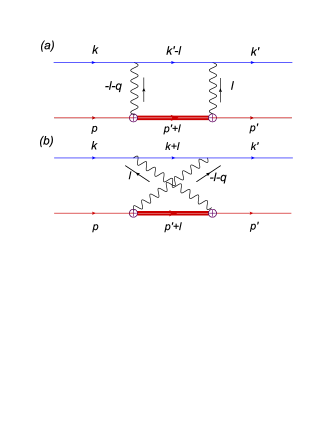
Figure 1: (Color online) Direct (a) and exchange (b) TPE box diagrams for elastic $ep$ scattering (Eq. 1). The intermediate states (thick double lines) are given by either the nucleon or the $P_{33}(1232)$ resonance.

Two photon exchange (TPE) effect in the elastic electron scattering off the proton has drawn back the attention of physicists about ten years ago, when the new experimental technique for measurement of the electromagnetic nucleon form-factors (FFs) had become available. In this method, called later polarization transfer (PT) technique, various polarization observables are measured and the form factor ratio,

$$\mathcal{R}_{1\gamma}(Q^{2})=\mu_{p}\frac{G_{E}(Q^{2})}{G_{M}(Q^{2})},$$ (1)

is estimated Ron:2011rdand_Puckett:2011xg . $G_{E}$ and $G_{M}$ are the electric and the magnetic proton form factors respectively, $\mu_{p}=2.793$ is the proton magnetic moment in the units of the nuclear magneton.

The proton electromagnetic FFs are also extracted from unpolarized cross section data (CS) by applying Rosenbluth (longitudinal-transverse (LT)) separation. As the result the electric and the magnetic FFs are obtained simultaneously. It turns out that the ratio (1) estimated basing on the Rosenbluth FFs data is inconsistent with the PT measurements at larger $Q^{2}$ values.

It is generally widely accepted that an insufficient estimate of the radiative corrections (RCs) applied in the Rosenbluth data analysis is a main source of inconsistency. In particular, it is argued that a lack of the so-called hard-photon TPE contribution coming from box diagrams drawn in Fig. 1 is responsible for the disagreement Blunden:2003sp ; Guichon:2003qm ; Chen:2004tw .

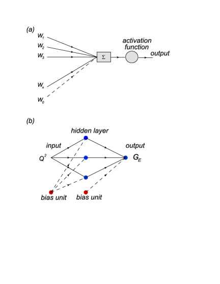
Figure 2: (Color online) In the top: single unit connected with $n$ units from the previous layer and with one bias unit ($\omega_{0}$ weight). In the bottom: simple MLP with one hidden layer, used to fit the electric proton form factor data

In the old Rosenbluth data analyses the cross section measurements were corrected by the RCs obtained by Mo and Tsai (MT) MT_radiative . In this approach the TPE corrections were calculated within a soft photon approximation. Supplementing this contribution by the hard photon correction changes the results of the Rosenbluth separation and makes them nearly consistent with the PT measurements Blunden:2003sp ; Blunden:2005ew .

Recently several theoretical calculations of the TPE correction have been performed Blunden:2003sp ; Blunden:2005ew ; Zhou:2009nf ; Kondratyuk:2005kk ; Kondratyuk:2006ig ; Borisyuk:2006fh ; Borisyuk:2008es ; Borisyuk:2012he ; Chen:2004tw ; Afanasev:2005mp ; Borisyuk:2008db ; Tjon:2009hf ; Kivel:2012vs ; Borisyuk:2013hja . They have been done within various approaches (for a review see Refs. Arrington:2011dn ; Carlson:2007sp ; Vanderhaeghen:2007zz ). It happens that the predictions of the TPE effect are mostly model-dependent at larger values of $Q^{2}$.

Simultaneously to the theoretical activity phenomenological investigations have been carried out as well. An effort has been made to extract the proton FFs and the TPE term directly from the experimental data Arrington:2003qk ; TomasiGustafsson:2004ms ; Tvaskis:2005ex ; Belushkin:2007zv ; Borisyuk:2007re ; Arrington:2007ux ; Chen:2007ac ; Alberico:2008sz ; TomasiGustafsson:2009pw ; Guttmann:2010au ; Venkat:2010by ; Graczyk:2011kh ; Qattan:2011ke ; Qattan:2011zz .

The TPE effect can be studied experimentally. The TPE correction for the elastic positron-proton scattering has an opposite sign but the same absolute value as the corresponding term in the electron-proton scattering. Hence the measurement of cross section ratio,

$$R_{+/-}=\frac{\displaystyle\frac{d\sigma}{d\Omega}(e^{+}p\to e^{+}p)}{\displaystyle\frac{d\sigma}{d\Omega}(e^{-}p\to e^{-}p)}\approx 1-2(\mathrm{TPE}),$$ (2)

gives a direct possibility to estimate the TPE correction. At present two dedicated $R_{+/-}$ measurement experiments are operating Bennett:2012zza ; Gramolin:2011tr . There is also a proposal of a new project, called OLYMPUS, in DESY Ice:2012zz .

In this report we would like to confront the phenomenological estimation of the TPE effect, obtained in our previous paper Graczyk:2011kh , with the theoretical predictions. In Ref. Graczyk:2011kh the global Bayesian analysis of the world elastic $ep$ data was performed. The major idea was to built a statistical model based on the experimental measurements with ability to make predictions of the electromagnetic proton FFs and the TPE term. It was achieved by adapting the Bayesian framework for the feed-forward neural networks (BNN) Graczyk:2010gw . This formalism allows one to perform the analysis as model-independent as possible. However, because the incompleteness of the data some additional assumptions had to be made. We applied constraints coming from the $C$-parity and the crossing symmetry invariance of the $ep$ scattering amplitude Rekalo:2003km ; Rekalo:2003xa ; Rekalo:2004wa . But the most important was to assume that for the PT data the TPE effect can be neglected and it is only relevant for the cross section data. This statement is supported both by general arguments Guichon:2003qm and calculations Blunden:2005ew ; Afanasev:2005mp . Indeed, the TPE corrections to the unpolarized cross section and the PT ratio $R_{1\gamma}$ data are comparable. But their inclusion in the Rosenbluth analysis affects significantly the results of the FFs extraction, while in the case of PT measurements TPE correction is of the order of statistical errors.

The comparison of BNN and the theoretical predictions allows one to verify validity of the model assumptions and to confront, in the non-direct way, theoretical model predictions with the data represented by the BNN.

In this paper the TPE corrections are computed in the similar way as in Refs. Blunden:2003sp ; Zhou:2009nf ; Kondratyuk:2005kk ; Kondratyuk:2006ig ; Blunden:2005ew , in a quantum-field theory approach, called later as hadronic model (HM). Hadronic intermediate states in the box diagrams (Fig. 1) are given by nucleon and $P_{33}(1232)$ resonance. Heavier resonances are not included because it was shown that their total contribution is negligible for these kinematics Kondratyuk:2006ig and their inclusion introduces the additional model-dependence to the discussion.

Our approach should work well at low and intermediate $Q^{2}$ range. Its input includes proton and $P_{33}(1232)$ electromagnetic FFs. For the proton we consider two different types of parametrizations. In contrast to the BNN analysis the FFs parameters are established from the global fit of HM to the unpolarized cross section data only. For the $N\to P_{33}$ electromagnetic transition we consider different vertex and FFs parametrizations than in Ref. Kondratyuk:2005kk .

In a wide $Q^{2}$ domain the BNN and the hadronic model predictions agree well. The discrepancy appears at low $Q^{2}$. However, the value of the proton radius extracted from the BNN fit is consistent with the recent atomic measurement by Pohl et al. Pohl:2010zza . It is shown that the low-$Q^{2}$ inconsistency between BNN and HM is induced by one of the model assumptions mentioned above (neglecting TPE correction to the PT data).

Eventually, we compare the predictions of the $R_{+/-}$ ratio obtained within the BNN and the HM approaches with the preliminary VEPP-3 measurements Gramolin:2011tr . The theoretical and the phenomenological predictions are in agreement with the new available data.

The paper is organized as follows. It contains six sections and two appendixes. In Sec. II the basic formalism is introduced. In Sec. III Bayesian neural network approach is shortly reviewed. The hadronic model is described in Sec. 8. Detailed comparison of the BNN and the theoretical predictions are presented in Sec. 11. We summarize our results in Sec. VI. Some technical details of the theoretical calculations are enclosed in Appendix A, while Appendix B contains the definition of $\chi^{2}$ function used in the data analysis.

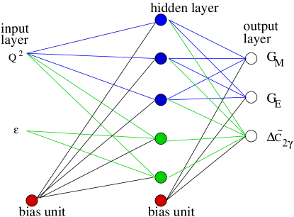
Figure 3: (Color online) Network $\mathcal{N}_{3,2}$: two input units, one layer of hidden units, three output units. The FF sector: blue filled units and connections; TPE sector: green units and connections. Each line corresponds to one weight parameter.

II Basic Formalism

We consider the elastic electron-proton scattering,

$$e(k)+p(p)\to p(p^{\prime})+e(k^{\prime}).$$ (3)

By $k$, $k^{\prime}$ and $p$, $p^{\prime}$ the initial and the final electron’s and proton’s four-momenta are denoted respectively. A four-momentum transfer is defined as $q=k-k^{\prime}$ and $q^{2}=(k-k^{\prime})^{2}=-Q^{2}$.

To compute the TPE correction we apply a typical approach to account for the radiative corrections in the $ep$ scattering Maximon:2000hm ; Blunden:2003sp . It is the quantum electrodynamics (QED) extended to include the hadronic degrees of freedom, like the proton and the $P_{33}(1232)$ resonance. The proton and nucleon electromagnetic vertices are expressed in terms of transition FFs.

The matrix element for the $ep$ scattering can be written as a perturbative series in $\alpha=e^{2}/4\pi\approx 1/137$. The first element of the series, $\mathcal{M}_{1\gamma}$, describes an exchange of one photon between the electron and the proton target, and it gives the lowest order contribution of the differential cross section, $d\sigma_{1\gamma}\sim\left|\mathcal{M}_{1\gamma}\right|^{2}.$ The $\mathcal{M}_{1\gamma}$ matrix element is a contraction of the one-body leptonic with hadronic currents,

$$i\mathcal{M}_{1\gamma}=i\frac{e^{2}}{Q^{2}}j^{\mu}h_{\mu}.$$ (4)

The leptonic and hadronic currents read,

$$j_{\mu}(q) = \overline{u}(k^{\prime})\gamma^{\mu}u(k),$$ (5)

$$h^{\mu}(q) = \overline{u}(p^{\prime})\Gamma^{\mu}(q)u(p).$$ (6)

$\Gamma^{\mu}$ is the on-shell proton electromagnetic vertex,

$$\Gamma^{\mu}(q) = \gamma^{\mu}F_{1}(Q^{2})+\frac{i\sigma^{\mu\nu}q_{\nu}}{2M_{p}}F_{2}(Q^{2}).$$ (7)

$F_{1}$ and $F_{2}$ are the Dirac and the spin flip proton form factors respectively, while $M_{p}=938$ MeV$/c^{2}$ is the proton mass. It is useful to express the above FFs in terms of the electric and the magnetic proton FFs.

$$F_{1}(Q^{2}) = \frac{1}{1+\tau}\left\{G_{E}(Q^{2})+\tau G_{M}(Q^{2})\right\},$$ (8)

$$F_{2}(Q^{2}) = \frac{1}{1+\tau}\left\{G_{M}(Q^{2})-G_{E}(Q^{2})\right\},$$ (9)

where $\tau={Q^{2}}/{4M^{2}_{p}}$.

We keep the normalization, $G_{E}(0)=1$, $G_{M}(0)=\mu_{p}$, hence $F_{1}(0)=1$, $F_{2}(0)=\kappa_{p}\equiv\mu_{p}-1$.

In the $ep$ scattering data analysis it is convenient to consider the reduced cross section, $\sigma_{R}$ ($d\sigma/d\Omega\sim\sigma_{R}$), which in Born approximation is given by the formula,

$$\sigma_{R,1\gamma}(Q^{2},\varepsilon)=\tau G_{M}^{2}(Q^{2})+\varepsilon G_{E}^{2}(Q^{2}),$$ (10)

where $\varepsilon$ is the photon polarization

$$\varepsilon=\left[1+2\left(1+\frac{Q^{2}}{4M_{p}^{2}}\right)\tan^{2}\!\left(\frac{\theta}{2}\right)\right]^{-1},$$ (11)

$\theta$ is the angle between the initial and the final electron momenta.

The next order terms of the cross section are given by the interference between $\mathcal{M}_{1\gamma}$ and second order amplitude $\mathcal{M}^{(2)}$. In the complete calculation, in order to remove the infrared (IR) divergences, the inelastic Bremsstrahlung contribution must be also taken into account,

$$d\sigma^{(2)} \sim 2\mathrm{Re}\left[(i\mathcal{M}_{1\gamma})^{*}i\mathcal{M}^{(2)}\right]+d\sigma_{Brem.}^{(1)}.$$ (12)

In this paper we focus on the TPE box diagrams (Fig. 1), which describe an exchange of two photons between the electron and the proton target. The intermediate hadronic state is the off-shell nucleon or a resonance. Because the off-shell electromagnetic form factors are not known off_shell_vertex we make a common ansatz and consider the on-shell vertices instead.

The leading TPE contribution reads,

$$\mathcal{I}_{2\gamma}\equiv 2\mathrm{Re}\left\{(i\mathcal{M}_{1\gamma})^{*}i\mathcal{M}_{2\gamma}\right\}.$$ (13)

The box diagrams contributing to $\mathcal{M}_{2\gamma}$ are drawn in Fig. 1.

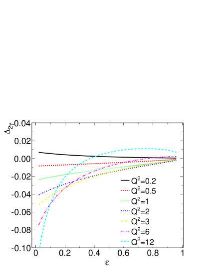
Figure 4: (Color online) $\Delta_{2\gamma}$ (Eq. 14) computed for $\Box(N)$ TPE contribution. The form factors from Ref. Blunden:2005ew are used. The values of $Q^{2}$ are in GeV² units.

In the old $ep$ data analysis to account for higher order radiative corrections MT approach MT_radiative was usually applied. In this approach the TPE box contribution was computed in the soft photon approximation. As it was pointed out by Blunden et al. Blunden:2003sp to properly correct the cross section data by ”full” TPE term, one has to subtract first the MT box contribution. Then the redefined TPE correction reads,

$$\Delta_{2\gamma}=\delta_{2\gamma}(full)-\delta_{2\gamma}(MT),$$ (14)

where

$$\delta_{2\gamma}=\frac{\mathcal{I}_{2\gamma}}{\displaystyle\left|i\mathcal{M}_{1\gamma}\right|^{2}},$$ (15)

and it is given by some integral, see Eq. 23 of Ref. Blunden:2005ew .

The inclusion of the TPE correcting term modifies the form of the reduced cross section, namely,

$$\sigma_{R,1\gamma+2\gamma}(Q^{2},\varepsilon)\to\sigma_{R,1\gamma}(Q^{2},\varepsilon)+\Delta C_{2\gamma}(Q^{2},\varepsilon),$$ (16)

where $\Delta C_{2\gamma}=\Delta_{TPE}\cdot\sigma_{R,1\gamma}.$

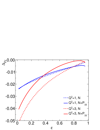
Figure 5: (Color online) $\Delta_{2\gamma}$ (Eq. 14) computed for either $\Box(N)$ or $\Box(N+P_{33})$ TPE contributions. The form factors from Ref. Blunden:2005ew are applied. The inelastic TPE correction, given by $\Box(P_{33})$, is computed within the $P_{33}(full)$ model. The values of $Q^{2}$ are in GeV² units.

III Neural Network Approach

The artificial neural networks (ANN) have been used in the particle and nuclear physics for many years. The ANNs are perfectly dedicated to particle or interaction identification and have been applied in the experimental data analyses NN_in_Physics . Study of the properties of ANNs is an interesting topic by itself. Neural networks have also been investigated within the methods of the statistical physics Hertz_book .

The feed-forward neural network is a type of the ANN, which can be applied to interpolating data, parameter estimation, and function approximation problems.

The ANN methodology can be a powerful approach for doing the approximation of the physical observables based on the measurements if it is difficult to make the predictions (base on the theoretical model) of the analysed quantities or the theoretical predictions are model-dependent but there exist the informative experimental data. Then one can construct a model-independent representation (given by neural network) of the physical observables favoured by the measurements. As an example let us mention the parton distributions functions (PDFs), which are parametrized by the feed-forward neural networks Ball:2013lla .

Similarly as in the case of the PDFs computing the nucleon FFs and the TPE correction from the first principles is a difficult task. On the other hand there are unpolarized cross section, ratio $R_{+/-}$ as well as PT ratio data distributed in the wide kinematical range. Global analysis of these measurements provide reliable information about the FFs and the TPE Arrington:2007ux ; Graczyk:2011kh .

The BNN approach was adapted by us Graczyk:2010gw ; Graczyk:2011kh to approximate the nucleon FFs and TPE correction. In the next four subsections a short review of the main features of this approach is presented.

III.1 Multi-Layer Perceptron

The FFs and TPE correction are going to be approximate by the feed-forward neural networks in the multi-layer perceptron (MLP) configuration. From the mathematical point of view the MLP, denoted as $\mathcal{N}$, is a non-linear function, which maps a subset of $\mathbb{R}^{n_{i}}$ (an input space) into $\mathbb{R}^{n_{o}}$ (an output space) where $n_{i},n_{o}\in\mathbb{N}$. Given MLP consists of several layers of units, namely, input, hidden and output layers (see Figs. 2 and 3).

A unit is a single-valued real function called an activation function $(f_{act.})$. For the argument it takes the weighted sum of outputs from the the previous layer units,

$$f_{act.}\left(\sum_{i=0}^{n}w_{i}f_{act.}^{i}(previous\;layer)\right),$$ (17)

where $w_{i}$ ($i=1,2,...,n$) is the weight parameter.

An example of the typical unit is drawn in Fig. 2. The weight parameters are established during the training i.e. a process of finding the optimal weight configuration. In reality the optimal weight configuration minimizes some error function.

In our analysis the sigmoid,

$$f_{act}(x)=\frac{1}{1+\exp(-x)}$$ (18)

is taken for the activation functions in the hidden layer. But in the case of the output units we consider the linear activation functions. The above choice is motivated by Cybenko theorem Cybenko_Theorem , which states that it is enough to consider the MLP with one hidden layer, and sigmoid-like functions there as well as the linear activation functions in the output layer to approximate any continuous function.

Notice that the effective support of (18) is limited. It is a useful feature in the case of the numerical analysis (the weights are randomly initialized at the beginning of every training).

For a more detailed description of the MLP properties, the training process, learning algorithms etc. see Sect. 2 of Ref. Graczyk:2010gw .

III.2 Overfitting Problem

A simple example of the one-hidden layer MLP configuration, used to approximate the electric proton FF Graczyk:2010gw , is shown in Fig. 2 (b). The input and output are the one-dimensional vectors, $(Q^{2})$ and $(G_{E})$ respectively. In this case the error function is postulated to be,

$$S_{ex}(\mathcal{D},\vec{w})=\chi^{2}=\sum_{i=1}^{N}\left(\frac{G_{E}(Q^{2}_{i};\vec{w})-G_{E,i}^{exp.}}{\Delta G_{E,i}^{exp.}}\right)^{2}.$$ (19)

$N$ denotes the number of experimental points, $(G_{E,i}^{exp.},\Delta G_{E,i}^{exp.})$ is the $i$th experimental point (its best value and error). By $\mathcal{{D}}$ the experimental data set (or sets) are denoted.

It is obvious that increasing the number of units (degrees of freedom) improves the ability of the network for representing the data. A MLP with large enough number of weight parameters may fit to the data exactly but in this case the statistical fluctuation of the measurements are reproduced. Such model has no predictive power and adding new data to the fit spoils its quality. This kind of the network overfits the data (or it is said the network is overlearned). Such fit is characterized by unrealistic prediction of the uncertainties (see discussion in Sect. 2.1 and Figs. 3 and 4 of Ref. Graczyk:2010gw ).

One of the methods for facing the overfitting problem and finding the optimal network configuration is to implement the Occam’s razor principle. Then in a natural way simpler network configurations are preferred. The simplest idea is to consider a penalty term,

$$\alpha E_{w},\quad\textrm{where}\;E_{w}=\frac{1}{2}\sum_{i=1}^{W}w_{i}^{2}.$$ (20)

Including in the error function the above expression may prevent from getting too large absolute values of the weight parameters and as the result the overlearned networks.

The parameter $\alpha$ in (19) is introduced to regularize the penalty term. In general one would consider several $\alpha$ parameters (each for every distinct class of weights), see e.g. Sect. 3.2 of Ref. Graczyk:2010gw or Chapter 9 of Ref. Bishop_book .

The major difficulty is to find an optimal value of the $\alpha$ parameter. The Bayesian framework offers mathematically consistent method for getting such $\alpha$’s. Indeed in this approach the penalty term has a natural probabilistic interpretation and $\alpha$ is computed within the objective Bayesian algorithm.

III.3 Bayesian Neural Networks

The bayesian framework for the MLP Bishop_book ; bayes was developed to provide consistent and objective methods, which allows one to:

• establish optimal structure of the MLP (number of the hidden units, layers);

• find optimal values of the weights and the $\alpha$ parameters;

• establish optimal values of the learning algorithm parameters;

• compute the neural network output uncertainty, and uncertainties for the weight and $\alpha$ parameters.

• classify and compare models quantitatively.

The BNN approach requires minimal input from the user. Indeed the idea of the approach was to replace the user’s common sense by the mathematical objective procedures Bishop_book . Obviously some user’s input is necessary.

Below we shortly review the BNN approach. For more detailed description of the BNN see Refs. Graczyk:2010gw (Sect. 3), Graczyk:2011kh (Sect. III) as well as Bishop_book and MacKay_thesis .

Model Comparison

Let us consider a set $\mathcal{S}$, which contains MLPs with different number of hidden units. Without loosing the generality of the approach we can restrict the set $S$ to the MLPs with only one hidden layer (the choice supported by Cybenko theorem). Each network $\mathcal{N}_{\beta}\in\mathcal{S}$ ($\beta=1,2,...$) approximates some physical quantities based on the data $\mathcal{D}$. The models (networks) can be classified by a conditional probability

$$P(\mathcal{N}_{\beta}|\mathcal{D}).$$ (21)

The BNN approach gives a recipe how to construct and compute the above function.

The Bayes’ theorem connects the probability (21) with the so-called evidence $P(\mathcal{D}|\mathcal{N}_{\beta})$,

$$P(\mathcal{N}_{\beta}|\mathcal{D})=\frac{P(\mathcal{D}|\mathcal{N}_{\beta})P(\mathcal{N}_{\beta})}{P(\mathcal{D})}.$$ (22)

$P(\mathcal{D})$ is the normalization factor, which does not depend on the model $\mathcal{N}_{\beta}$. $P(\mathcal{N}_{\beta})$ is the prior probability. However, at the beginning of any analysis there is no reason to prefer a particular model (network) therefore it is natural to assume that,

$$P(\mathcal{N}_{1})=P(\mathcal{N}_{2})=P(\mathcal{N}_{3})=...$$ (23)

Hence the evidence differs from $P(\mathcal{N}_{\beta}|\mathcal{D})$ by only a constant normalization factor and it can be used to qualitatively classify the statistical hypotheses.

We apply the so-called hierarchical approach MacKay_thesis to construct and then to compute the evidence. It is several steps procedure, which is described in the next four subsections.

First Step

In the first step of the approximation the posterior probability distribution $P(\vec{w}|\mathcal{D},\alpha,\mathcal{N}_{\beta})$ is computed. According to the Bayes’ theorem it reads,

$$P(\vec{w}|\mathcal{D},\alpha,\{\mathcal{I}_{Phys.}\},\mathcal{N}_{\beta}) =$$ (24)

$$\!\!\!\!\!\!\!\!\!\!\!\!\!\!\!\!\!\!\!\!\!\!\!\!\!\!\!\!\!\!\!\!\!\!\!\!\!\!\!\!\!\!\!\!\!\!\!\!\!\!\!\!\!\!\!\!\!\!\!\!\!\!\!\!\!\!\!\!\!\!\!\!\!\!\!\!\!\!\!\!\!\!\!\!\!\!\!\frac{\mathcal{P}\left(\mathcal{D}\right|\left.\vec{w},\alpha,\{\mathcal{I}_{Phys.}\},\mathcal{N}_{\beta}\right)\mathcal{P}\left(\vec{w}\right|\left.\alpha,\{\mathcal{I}_{Phys.}\},\mathcal{N}_{\beta}\right)}{\mathcal{P}\left(\mathcal{D}\right|\left.\alpha,\{\mathcal{I}_{Phys.}\},\mathcal{N}_{\beta}\right)},$$

where $\mathcal{P}\left(\vec{w}\right|\left.\alpha,\{I\}_{Phys.},\mathcal{N}_{\beta}\right)$ is the prior probability, $\{\mathcal{I}\}_{Phys.}$ denotes the set of initial physical assumptions.

The likelihood function, $\mathcal{P}\left(\mathcal{D}\right|\left.\vec{w},\alpha,\{\mathcal{I}_{Phys.}\},\mathcal{N}_{\beta}\right)$ does not depend on $\alpha$ but in our analysis it is modified due to the physical constraints $\{\mathcal{I}\}_{Phys.}$,

$$\mathcal{P}\left(\mathcal{D}\right|\left.\vec{w},\mathcal{N}_{\beta},\{\mathcal{I}\}_{Phys.}\right) =$$ (25)

$$\!\!\!\!\!\!\!\!\!\!\!\!\!\!\!\!\!\!\!\!\!\!\!\!\!\!\!\!\!\!\!\!\!\!\!\!\!\!\!\!\!\!\!\!\!\!\!\!\!\!\!\!\!\!\!\!\!\!\!\!\!\!\!\!\frac{1}{n_{\beta}}\exp\left(-S_{ex}(\mathcal{D},\vec{w})-S_{Phys.}(\{\mathcal{I}_{Phys.}\},\vec{w})\right).$$

The normalization factor $n_{\beta}$ is computed in Hessian approximation, see Eq. (3.8) of Ref. Graczyk:2010gw .

The functions $S_{ex}(\mathcal{D},\vec{w})$ and $S_{Phys.}(\{\mathcal{I}_{Phys.}\},\vec{w})$ are given by some $\chi^{2}$ distributions. $S_{Phys.}(\{\mathcal{I}_{Phys.}\},\vec{w})$ is introduced to force the MLP to properly reproduce the form factors at $Q^{2}=0$. (see Sec. III of Ref.Graczyk:2011kh ). It may also account for other physical constraints.

The prior $\mathcal{P}\left(\vec{w}\right|\left.\mathcal{N}_{\beta}\right)$ describes only the initial ANN assumptions about the weights. A reasonable approximation is to assume that it is given by the normal distribution, centred at $\vec{w}_{0}=\vec{0}$.

$$\mathcal{P}\left(\vec{w}\right|\left.\alpha,\mathcal{N}_{\beta}\right) = \frac{1}{n_{a}}\exp[-\alpha E_{w}]$$ (26)

$$n_{a} = \int d^{W_{\beta}}w\exp[-\alpha E_{w}].$$ (27)

The optimal configuration of weights $\vec{w}_{MP}$ maximizes the posterior probability (24). In reality it minimizes the following error function,

$$S_{ex}(\mathcal{D},\vec{w})+S_{Phys.}(\{\mathcal{I}_{Phys.}\},\vec{w})+\alpha E_{w}.$$ (28)

Notice that in this step of the approximation the $\alpha$ parameter is assumed to be known.

The $1\sigma$ error of any physical observable $\mathcal{O}$, which depends on the network response is a square root of the variance,

$$\left(\langle\Delta\mathcal{O}\rangle\right)^{2} = \langle\mathcal{O}^{2}\rangle-\langle\mathcal{O}\rangle^{2}$$

$$\langle\mathcal{O}\rangle = \int d^{W_{\beta}}w\,\mathcal{O}(\mathcal{N}_{\beta})P(\vec{w}|\mathcal{D},\alpha,\{\mathcal{I}_{Phys.}\},\mathcal{N}_{\beta}).$$

The above integral is computed in the Hessian approximation.

Second Step

The optimal value of the $\alpha$ parameter $(\alpha_{MP})$ maximizes the posterior probability,

$$\mathcal{P}\left(\alpha\right|\left.\mathcal{D},\{\mathcal{I}_{Phys.}\},\mathcal{N}_{\beta}\right) =$$ (30)

$$\!\!\!\!\!\!\!\!\!\!\!\!\!\!\!\!\!\!\!\!\!\!\!\!\!\!\!\!\!\!\!\!\!\!\!\!\!\!\!\!\!\!\!\!\!\!\!\!\!\!\!\!\!\!\!\!\!\!\!\!\!\!\frac{\mathcal{P}\left(\mathcal{D}\right|\left.\alpha,\{\mathcal{I}_{Phys.}\},\mathcal{N}_{\beta}\right)\mathcal{P}\left(\alpha\right|\left.\{\mathcal{I}_{Phys.}\},\mathcal{N}_{\beta}\right)}{\mathcal{P}\left(\mathcal{D}\right|\left.\{\mathcal{I}_{Phys.}\},\mathcal{N}_{\beta}\right)}.$$

(the denominator of the above expression is obtained in the previous step of the approximation).

The necessary condition, which must by satisfied by $\alpha_{MP}$ reads,

$$\left.\frac{\partial}{\partial\alpha}\mathcal{P}\left(\alpha\right|\left.\mathcal{D},\mathcal{N}_{\beta}\right)\right|_{\alpha=\alpha_{MP}}=0.$$ (31)

It can be shown that in the Hessian approximation the above equation can be written as,

$$2\alpha_{MP}E_{w}(\vec{w}_{MP})=\sum_{i=1}^{W_{\beta}}\frac{\lambda_{i}}{\lambda_{i}+\alpha_{MP}}\equiv\gamma(\alpha_{MP}),$$ (32)

where $\lambda_{i}$ are the eigenvalues of $H_{kj}=\nabla_{k}\nabla_{j}(S_{ex}+S_{Phys.})$, $k,j=1,...,W_{\beta}$, $\nabla_{k}\equiv\partial/\partial w_{k}$.

In practice $\lambda_{i}$’s depend on $\alpha$. Hence to get the optimal $\alpha_{MP}$, the value of $\alpha$ is iteratively changed during the training, $\alpha_{k+1}=\gamma(\alpha_{k})/2E_{w}$. It means that the optimal weights and $\alpha$ parameter are established during the same training process.

The initial value of the $\alpha$ parameter is taken to be large, which corresponds to the prior assumption that at the beginning of the analysis almost all relevant values of weights are probable.

Third Step

In this step the evidence is computed. Notice that it is the denominator of right-hand side of Eq. 30. Careful calculations leads to the following expression for log of evidence (see Sect 3.1 of Ref. Graczyk:2010gw ),

$$\ln\mathcal{P}\left(\mathcal{D}\right|\left.\{\mathcal{I}_{Phys.}\},\mathcal{N}_{\beta}\right) =$$ (35)

$$\!\!\!\!\!\!\!\!\!\!\!\!\!\!\!\!\!\!\!\!\!\!\!\!\!\!\!\!\!\!\!\!\!\!\!\!\!\!\!\!\!\!\!\!\!\!\!\!\!\!\!\!\!\!\!\!\!\!\!\!-S_{ex}(\mathcal{D},\vec{w}_{MP})-S_{Phys.}(\{\mathcal{I}_{Phys.}\},\vec{w}_{MP})$$

$$\!\!\!\!\!\!\!\!\!\!\!\!\!\!\!\!\!\!\!\!\!\!\!\!\!\!\!\!\!\!\!\!\!\!\!\!\!\!\!\!\!\!\!\!\!\!\!\!\!\!\!\!\!\!\!\!\!\!\!\!\!\!\!-\alpha_{MP}E_{w}(\vec{w}_{MP})-\frac{1}{2}\ln\mathrm{det}A+\frac{W}{2}\ln\alpha_{MP}-\frac{1}{2}\ln\frac{\gamma}{2}$$

$$\!\!\!\!\!\!\!\!\!\!\!\!\!\!\!\!\!\!\!\!\!\!\!\!\!\!\!\!\!\!\!\!\!\!\!\!\!\!\!\!\!\!\!\!\!\!\!\!\!\!\!\!\!\!\!\!\!\!\!\!\!\!\!+(g+t)\ln(2)+\ln(g!)+\ln(t!),$$

$A=H(\vec{w}_{MP})+\alpha_{MP}I$.

Expression (35) is the misfit of the approximated data. It is usually of the low-value. Terms (LABEL:evidence_Occam_volume-35) contribute to the Occam’s factor. Indeed (LABEL:evidence_Occam_volume) takes large values for the models, which overfit the data. In a typical MLP some hidden units, in the given layer, can be reordered without affecting the values of the network output. It means that for every MLP there exist several equivalent indistinguishable network configurations. It gives rise to the additional normalization factor (35), which must be included to properly define the evidence. The symmetry factor presented above concerns the MLP used in the extraction of the TPE correction from the data (see Sect. III.4 and Eq. 39).

General Scheme

Schematically the approach discussed above can be summarized as follows,

$$1th\;Step: \to P(\vec{w}|\mathcal{D},\alpha,\{\mathcal{I}_{Phys.}\},\mathcal{N}_{\beta})$$ (36)

$$2d\;Step: \to \mathcal{P}\left(\alpha\right|\left.\mathcal{D},\{\mathcal{I}_{Phys.}\},\mathcal{N}_{\beta}\right)$$ (37)

$$3d\;Step: \to \mathcal{P}\left(\mathcal{D}\right|\left.\{\mathcal{I}_{Phys.}\},\mathcal{N}_{\beta}\right)$$ (38)

We see that the evidence, and the other posterior probabilities may depend on physical assumptions. Obviously their impact on the final results must be carefully discussed.

III.4 Extraction of TPE

The formalism discussed above was applied to extract the proton FFs and TPE correction Graczyk:2011kh from the world elastic $e^{-}p$ and $e^{+}p$ scattering data. We utilized the unpolarized cross section, ratio $R_{+/-}$ and PT data. The first two types of observables depend on two input variables $Q^{2}$ and $\epsilon$, while the last one depends only on $Q^{2}$.

On the other hand the TPE correction is a function of two input variables, but the FFs depend on $Q^{2}$ only. This property was encoded in the network configuration by dividing MLP into two sectors (see Fig. 3). In the first there are $g$ units connected only with the $Q^{2}$ input, while in the other there are $t$ units connected with both input units. We denote this network as,

$$\mathcal{N}_{g,t}\left(\pmatrix{Q^{2}\cr\varepsilon};\vec{w}\right)=\pmatrix{G_{E}^{\mathcal{N}}\cr G_{M}^{\mathcal{N}}\cr\Delta\tilde{C}_{2\gamma}^{\mathcal{N}}}.$$ (39)

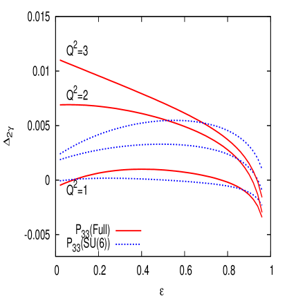
Figure 6: (Color online) $\Delta_{2\gamma}$ (Eq. 14) given by the resonance $P_{33}$ contribution only. Calculations are done for the $P_{33}(\mathrm{SU}(6))$ and $P_{33}(full)$ models. The values of $Q^{2}$ are in GeV² units.

The BNN formalism seems to be well suited for performing a model-independent analysis but because the utilized data turned out to be not informative enough some model assumptions had to be made.

The main constraint was induced by the following assumption,

1. The PT data is less sensitive to the TPE correction than the cross section measurements Guichon:2003qm , hence the TPE contribution to $\mathcal{R}_{1\gamma}$ ratio can be neglected.

As a consequence the TPE correcting term was considered only in the case of the unpolarized cross section and $R_{+/-}$ data. Its extraction was induced by the presence of the PT measurements in the fit. Certainly it is an approximation, therefore we distinguish between $\Delta C_{2\gamma}$, as it is defined by theory, and $\Delta\tilde{C}_{2\gamma}$ as it is given by the BNN analysis. Both quantities enter the reduced cross section formula in the same way, see Eq. 16. But the latter is needed to get a consistent fit of the CS, $R_{+/-}$ and PT.

To get the FFs properly behaved at $Q^{2}=0$, and TPE term at $\epsilon=0$ (as it is suggested by the C-invariance Rekalo:2003km ; Rekalo:2003xa ; Rekalo:2004wa ), we introduced $S_{Phys.}$ (Eq. 28). It was a $\chi^{2}$ function containing three artificial points (for details see Sect. III of Ref. Graczyk:2011kh ).

In order to find the optimal MLP configuration 45 different configurations of MLPs were trained. The largest evidence was obtained for the model $\mathcal{N}_{5,6}$.

In general the optimal fit should be given by an average (weighted by evidence) over all hypothetical models. In this case the physical observable $\mathcal{F}$, which is a function of FFs and TPE, reads,

$$\langle\mathcal{F}(G_{E},G_{M},\Delta\tilde{C}_{2\gamma})\rangle =$$ (40)

$$\!\!\!\!\!\!\!\!\!\!\!\!\!\!\!\!\!\!\!\!\!\!\!\!\!\!\!\!\!\!\!\!\!\!\!\int_{\mathcal{S}}D\mathcal{N}\mathcal{F}(G_{E}^{\mathcal{N}},G_{M}^{\mathcal{N}},\Delta\tilde{C}_{2\gamma}^{\mathcal{N}})\mathcal{P}(\mathcal{N}|\mathcal{D}).$$

In reality the above integral can be written as discrete series,

$$\left\langle\mathcal{F}(G_{E},G_{M},\Delta\tilde{C}_{2\gamma})\right\rangle =$$ (41)

$$\!\!\!\!\!\!\!\!\!\!\!\!\!\!\!\!\!\!\!\!\!\!\!\!\!\!\!\!\!\!\!\!\!\!\!\!\!\!\!\!\!\!\!\!\!\!\!\!\!\!\!\!\!\!\!\!\!\!\!\!\!\!\!\!\!\!\!\!\!\!\!\!\sum_{m=1}^{M}\sum_{g=1,t=1}^{g+t=m}\mathcal{F}(G_{E}^{\mathcal{N}_{g,t}},G_{M}^{\mathcal{N}_{g,t}},\Delta\tilde{C}_{2\gamma}^{\mathcal{N}_{g,t}})\mathcal{P}(\mathcal{N}_{g,t}|\mathcal{D}),$$

where $M\in\mathbb{N}$.

It turned out that the evidence for $\mathcal{N}_{5,6}$ model was much larger then for the other analysed configurations of networks. Hence the expression (41) contains only one dominant term,

$$\left\langle\mathcal{F}(G_{E},G_{M},\Delta\tilde{C}_{2\gamma})\right\rangle\approx\mathcal{F}(G_{E}^{\mathcal{N}_{5,6}},G_{M}^{\mathcal{N}_{5,6}},\Delta\tilde{C}_{2\gamma}^{\mathcal{N}_{5,6}}).$$ (42)

IV Hadronic Calculations

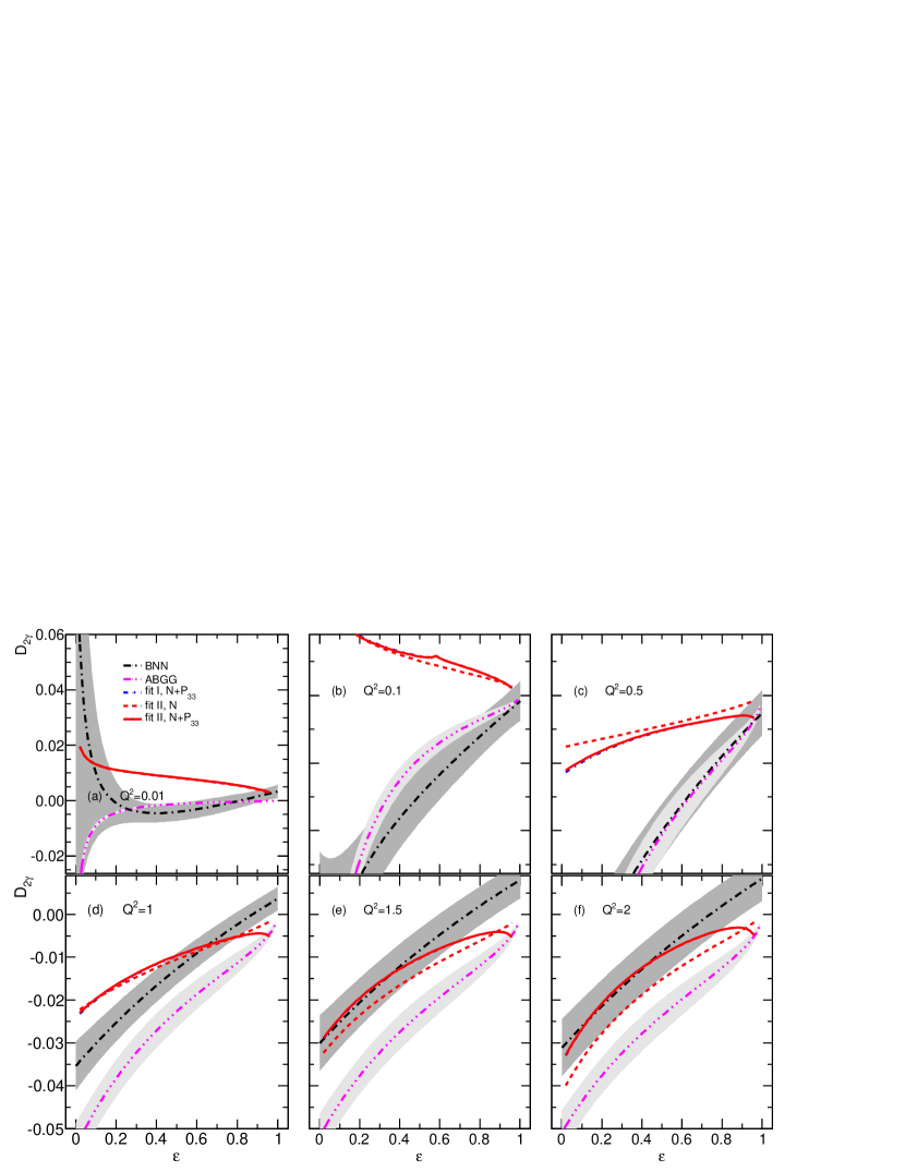
Figure 7: (Color online) Predictions of $D_{2\gamma}$ (Eq. 64) based on the BNN and HM (fits I and II) as well as ABGG approaches. The TPE correction includes either elastic $(N)$ or elastic and $P_{33}$ resonance (full model) contributions. The values of $Q^{2}$ are in GeV² units. The shaded areas show $1\sigma$ error computed from the covariance matrix.

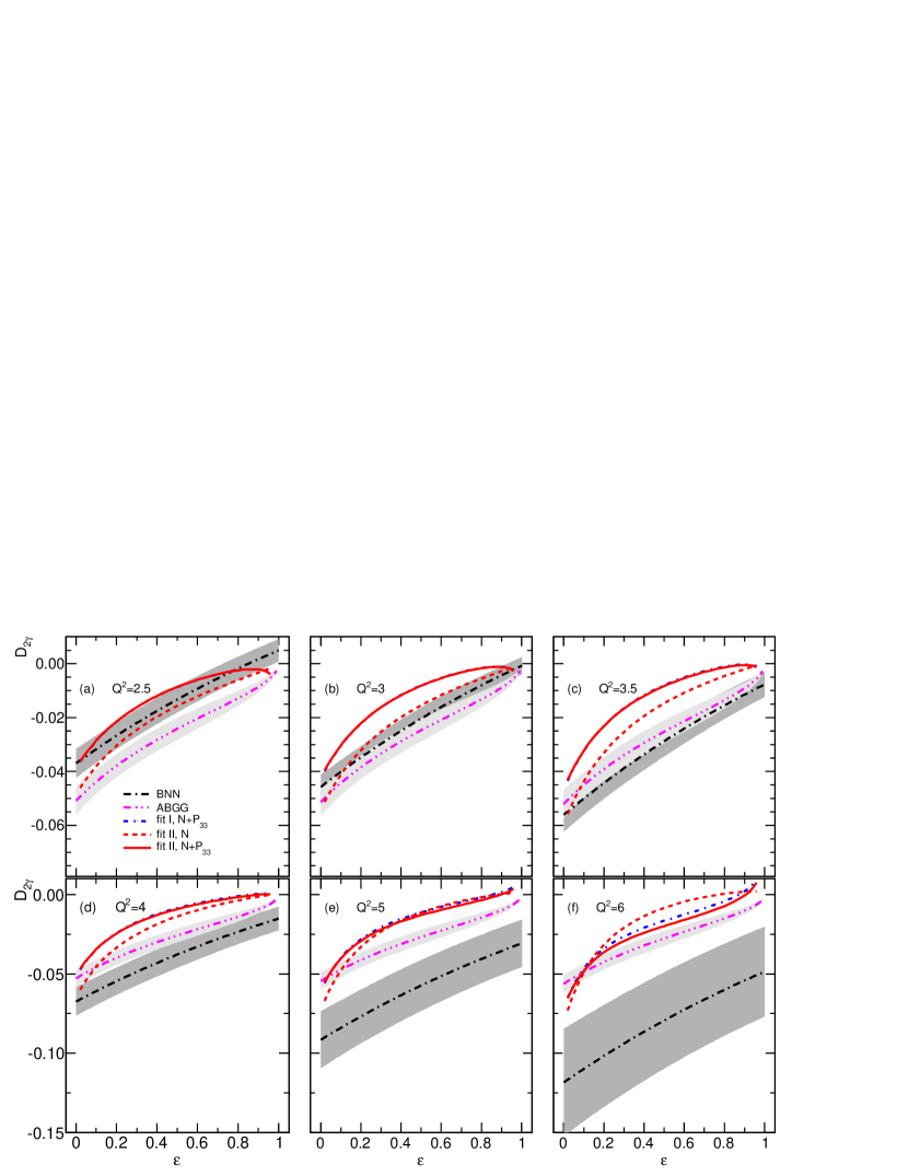
Figure 8: (Color online) Caption the same as in Fig. 7.

IV.1 Box Diagrams

The TPE correction is computed in the similar way as in Refs. Maximon:2000hm ; Blunden:2003sp ; Blunden:2005ew ; Kondratyuk:2005kk ; Zhou:2009nf ; Tjon:2009hf . Four box diagrams contribute to the $2\gamma$ amplitude (see Fig. 1): two with the nucleon intermediate hadronic state (denoted as $\Box(N)$) and two with $P_{33}(1232)$ hadronic intermediate state (denoted as $\Box(P_{33})$). The TPE contribution (13) reads,

$$\mathcal{I}_{2\gamma}=2\frac{e^{2}}{Q^{2}}\mathrm{Im}\left\{w_{N}^{\parallel}+w_{N}^{\times}+w_{\Delta}^{\parallel}+w_{\Delta}^{\times}\right\},$$ (43)

$w_{N,\Delta}^{\parallel}$ and $w_{N,\Delta}^{\times}$ are the one-loop integrals represented by direct and exchange $\Box(N)$ and $\Box(P_{33})$ diagrams respectively,

$$w_{N,\Delta}^{\parallel} = e^{4}\int\frac{d^{4}l}{(2\pi)^{4}}\frac{\displaystyle L^{\alpha\mu\nu}_{\parallel}\mathcal{H}^{N,\Delta}_{\alpha\mu\nu}}{D(-k^{\prime})}$$ (44)

$$w_{N,\Delta}^{\times} = e^{4}\int\frac{d^{4}l}{(2\pi)^{4}}\frac{\displaystyle L^{\alpha\mu\nu}_{\times}\mathcal{H}^{N,\Delta}_{\alpha\mu\nu}}{D(k)},$$ (45)

where

$$D(x) = [(q+l)^{2}+i\epsilon][l^{2}+i\epsilon]\times$$ (46)

$$\!\!\!\!\!\!\!\!\!\!\!\!\!\!\!\!\!\!\!\!\![(l+x)^{2}-m^{2}+i\epsilon][(p^{\prime}+l)^{2}-M^{2}_{p,\Delta}+i\epsilon].$$

We keep a nonzero electron mass $m=0.510$ MeV$/c^{2}$. $M_{\Delta}=1232$ MeV$/c^{2}$ denotes the $P_{33}$ resonance mass. The numerators of integrals (44) and (45) are given by the contraction of three-dimensional leptonic with hadronic tensors.

The leptonic tensor is defined as follows,

$$L^{\alpha\mu\nu}_{\parallel,\times}\equiv\sum_{spin}j^{\alpha*}j^{\mu\nu}_{\parallel,\times},$$ (47)

where

$$j^{\mu\nu}_{\parallel} = \overline{u}(k^{\prime})\gamma^{\mu}(\hat{k^{\prime}}-\hat{l}+m)\gamma^{\nu}u(k)$$ (48)

$$j^{\mu\nu}_{\times} = \overline{u}(k^{\prime})\gamma^{\mu}(\hat{k}+\hat{l}+m)\gamma^{\nu}u(k),$$ (49)

$$\hat{x} = x_{\mu}\gamma^{\mu}.$$ (50)

Four-vector $j^{\alpha}$ is given by Eq. (5).

We distinguish two types of the hadronic tensors, one for the nucleon and another for the $P_{33}$ intermediate state,

$$\mathcal{H}^{N,\Delta}_{\alpha\mu\nu} \equiv \sum_{spin}h_{\alpha}^{*}h_{\mu\nu}^{N,\Delta},$$ (51)

where $h_{\alpha}$ is given by Eq. (6) and

$$h_{\mu\nu}^{N}=\overline{u}(p^{\prime})\Gamma_{\nu}(-l)(\hat{p^{\prime}}+\hat{l}+M_{p})\Gamma_{\mu}(q+l)u(p).$$ (52)

The proton electromagnetic vertex $\Gamma_{\mu}$ is defined by Eq. 7. The hadronic tensor for the $\Box(P_{33})$ diagrams has the form,

$$h_{\mu\nu}^{\Delta} = \overline{u}(p^{\prime})\Gamma_{\mu\xi}^{\Delta,in}(-l,p^{\prime}+l)\left(\hat{p^{\prime}}+\hat{l}+M_{\Delta}\right)$$ (53)

$$\quad\Lambda^{\xi\eta}(p^{\prime}+l)\Gamma_{\nu\eta}^{\Delta,out}(q+l,p^{\prime}+l)u(p).$$

$\Gamma_{\nu\mu}^{\Delta,out}(q_{\Delta},P)$ and $\Gamma_{\nu\mu}^{\Delta,in}(q_{\Delta},P)$ denote the vertex for the $\gamma^{*}N\to\Delta$ and $\Delta\to N\gamma^{*}$ transitions. For more detailed definitions see Sec. IV.3.

For the Rarita-Schwinger $3/2$ spin field propagator we take,

$$S_{\mu\nu}^{\Delta}=-\frac{i(\hat{p}+M_{\Delta})}{p^{2}-M_{\Delta}^{2}+i\Gamma_{\Delta}M_{\Delta}}\Lambda_{\mu\nu}(p).$$ (54)

Similarly as Kondratyuk et al. Kondratyuk:2005kk we set $\Gamma_{\Delta}\to 0$. With this simplification the dominant contribution to the loop integrals comes from the $P_{33}$ resonance mass pole. Hence the choice of on-shell projection operator,

$$\Lambda_{\mu\nu}(p)=g_{\mu\nu}-\frac{1}{3}\gamma_{\mu}\gamma_{\nu}-\frac{2p_{\mu}p_{\nu}}{3M_{\Delta}^{2}}+\frac{p_{\mu}\gamma_{\nu}-p_{\nu}\gamma_{\mu}}{3M_{\Delta}},$$ (55)

leads to the same results as the off-shell projection operator discussed by Kondratyuk et al.. Taking into consideration this approximation for projector operator simplifies and also accelerates the algebraic decomposition of the integrals (44) and (45). The procedure of computing the integrals (44-45) is described in the Appendix A.

IV.2 Nucleon Form Factors

For the nucleon FFs we consider two parametrizations:

• parametrization I, sum of three monopoles,

  $$F_{k}(Q^{2})=\sum_{i=1}^{3}\frac{f_{i}^{k}}{m_{i}^{k}+Q^{2}},$$ (56)

  where $f^{1}_{3}=m^{1}_{3}(1-f^{1}_{1}/m^{1}_{1}-f^{1}_{2}/m^{1}_{2})$, $f^{2}_{3}=m^{2}_{3}(\kappa_{p}-f^{2}_{1}/m^{2}_{1}-f^{2}_{2}/m^{2}_{2})$;

• parametrization II, sum of three dipoles,

  $$F_{k}(Q^{2})=\sum_{i=1}^{3}{f_{i}^{k}}\left(1+\frac{Q^{2}}{(m_{i}^{k})^{2}}\right)^{-2},$$

  where $f_{3}^{1}=1-f_{1}^{1}-f_{2}^{1}$, $f_{3}^{2}=\kappa_{p}-f_{1}^{2}-f_{2}^{2}$.

The parametrization I was previously discussed by Blunden, et al. Blunden:2005ew (BMT05). In order to cross check our algebraical and numerical procedures we repeat and check the calculations done in Blunden:2005ew . In Fig. 4 we present predictions for $\Delta_{2\gamma}$ obtained for the same kinematics and the form factors as in BMT05 paper (for comparison see the plots in Figs. 2 and 3a of Ref. Blunden:2005ew ). We notice the excellent agreement between our hadronic model and the BMT05 predictions.

The $\Delta_{2\gamma}$ (or $D_{2\gamma}$) function depends weakly on the proton form factors parametrization. Small differences between TPE predictions based on the parametrizations I and II appear for larger values of $Q^{2}$ (see Figs. 7 and 8). But this is the region where the validity of the theoretical approach can questionable.

IV.3 $P_{33}(1232)$ Form Factors

The hadronic vertex, $\Gamma_{\mu\nu}^{\Delta,out}(q,P_{\Delta})$ for $\gamma^{*}p\to\Delta^{++}$ transition is obtained by assuming that $P_{33}$ resonance is described by the Rarita-Schwinger 3/2 spin field,

$$\overline{\Psi}^{\nu}(P)\Gamma_{\mu\nu}^{\Delta,out}(q,P)u(p),\quad q=P-p.$$ (57)

One of the commonly discussed vertex parametrizations is the following Jones:1972ky ,

$$\Gamma_{\mu\nu}^{\Delta,out}(q\equiv P-q,P) = \left[\frac{C_{5}^{V}}{M^{2}}(g_{\mu\nu}p\cdot q-{p}_{\mu}{q}_{\nu})\right.$$

$$\!\!\!\!\!\!\!\!\!\!\!\!\!\!\!\!\!\!\!\!\!\!\!\!\!\!\!\!\!\!\!\!\!\!\!\!\!\!\!\!\!\!\!\!\!\!\!\!\!\!\!\!\!\!\!\!\!\!\!\!\!\!\!\!\!\!\left.+\frac{C_{4}^{V}}{M^{2}}(g_{\mu\nu}q\cdot{P}-{P}_{\mu}q_{\nu})+\frac{C_{3}^{V}}{M}(g_{\mu\nu}\hat{q}-\gamma_{\mu}{q}_{\nu})\right]\gamma_{5}.$$

$P$ is the four-momentum of the outgoing $P_{33}$ resonance, while $p$ denotes the four-momentum of the incoming proton.

The $\Delta^{++}\to\gamma^{*}p$ vertex reads Kondratyuk:2005kk ,

$$\Gamma_{\mu\nu}^{\Delta,in}(p,P_{\Delta})=\gamma_{0}\left(\Gamma_{\mu\nu}^{\Delta,out}(p,P_{\Delta})\right)^{\dagger}\gamma_{0}.$$ (59)

For the $N\to P_{33}$ transition form factors we consider two scenarios,

• $P_{33}({\mathrm{SU}(6)})$ model: there is only one vector form factor $C_{3}^{V}$; two other are obtained assuming $\mathrm{SU}(6)$ quark model relations Liu:1995bu , namely,

  $$C_{5}^{V}(Q^{2})=0,\quad C_{4}^{V}(Q^{2})=-\frac{M}{M_{\Delta}}C_{3}^{V}(Q^{2}).$$ (60)

  In this case we parametrize the $C_{3}^{V}(Q^{2})$ form factor as follows AlvarezRuso:1998hi ,

  $$C_{3}^{V}(Q^{2})=\frac{2.05}{\displaystyle\left(1+\frac{Q^{2}}{0.54\,\mathrm{GeV}^{2}}\right)^{2}}.$$ (61)

• $P_{33}({Full})$ model: we apply the form factors from Ref. Lalakulich:2006sw , namely,

  $$C_{i}^{V}(Q^{2})=c_{i}^{V}\left(1+\frac{Q^{2}}{a_{i}M_{V}^{2}}\right)^{-1}G_{D}(Q^{2}),$$ (62)

  where $a_{3}=a_{4}=4$, $a_{5}=0.776$, $c_{3}^{V}=2.13$, $c_{4}^{V}=-1.51$, $c_{5}^{V}=0.48$,

  $$G_{D}(Q^{2})=\left(1+\frac{Q^{2}}{M_{V}^{2}}\right)^{-2},\quad\mathrm{and}\quad M_{V}=0.84~{}\mathrm{GeV}.$$ (63)

In the wide $Q^{2}$ range (for $Q^{2}>0.1$ GeV² the form factors given by Eq. (62) take the similar values as MAID07 form factors Drechsel:2007if .

The $P_{33}(full)$ model is different than the one applied by Kondratyuk et al. Kondratyuk:2005kk (denoted as KBMT05). However, in the intermediate $Q^{2}$ range the predictions are comparable, as seen in comparing our Fig. 5 with Fig. 2 from Ref. Kondratyuk:2005kk ). We notice also a qualitative agreement with predictions Borisyuk and Kobushkin model Borisyuk:2012he . In both approaches the TPE $\Box(P_{33})$ correction is positive at low and intermediate $Q^{2}$ range and it reduces the total TPE correction.

In contrast to $\Delta_{2\gamma}(N)$, the function $\Delta_{2\gamma}(P_{33})$ depends on the details of the hadronic model. Indeed, there are small but noticeable differences between predictions KBMT05 and $P_{33}(full)$ model. To illustrate the model dependence of $\Delta_{2\gamma}(P_{33})$ the prediction of TPE correction obtained within $P_{33}(\mathrm{SU}(6))$ and $P_{33}(full)$ models are plotted in Fig. 6. There is a clear discrepancy between predictions of both approaches.

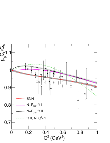
Figure 9: (Color online) Ratio $\mu_{p}G_{E}/G_{M}$ calculated based on fits I and II ($N$ and resonance $P_{33}$ contributions) as well as BNN fit. Additionally ratio $\mu_{p}G_{E}/G_{M}$ obtained based on the fit (parametrization II) to the unpolarized cross section data below $Q^{2}=1$ GeV² is also plotted. The PT data (points with error bars) are taken from Ref. PT_data and Zhan et al. Zhan:2011ji (open diamonds). The shaded areas show $1\sigma$ error computed from the covariance matrix.

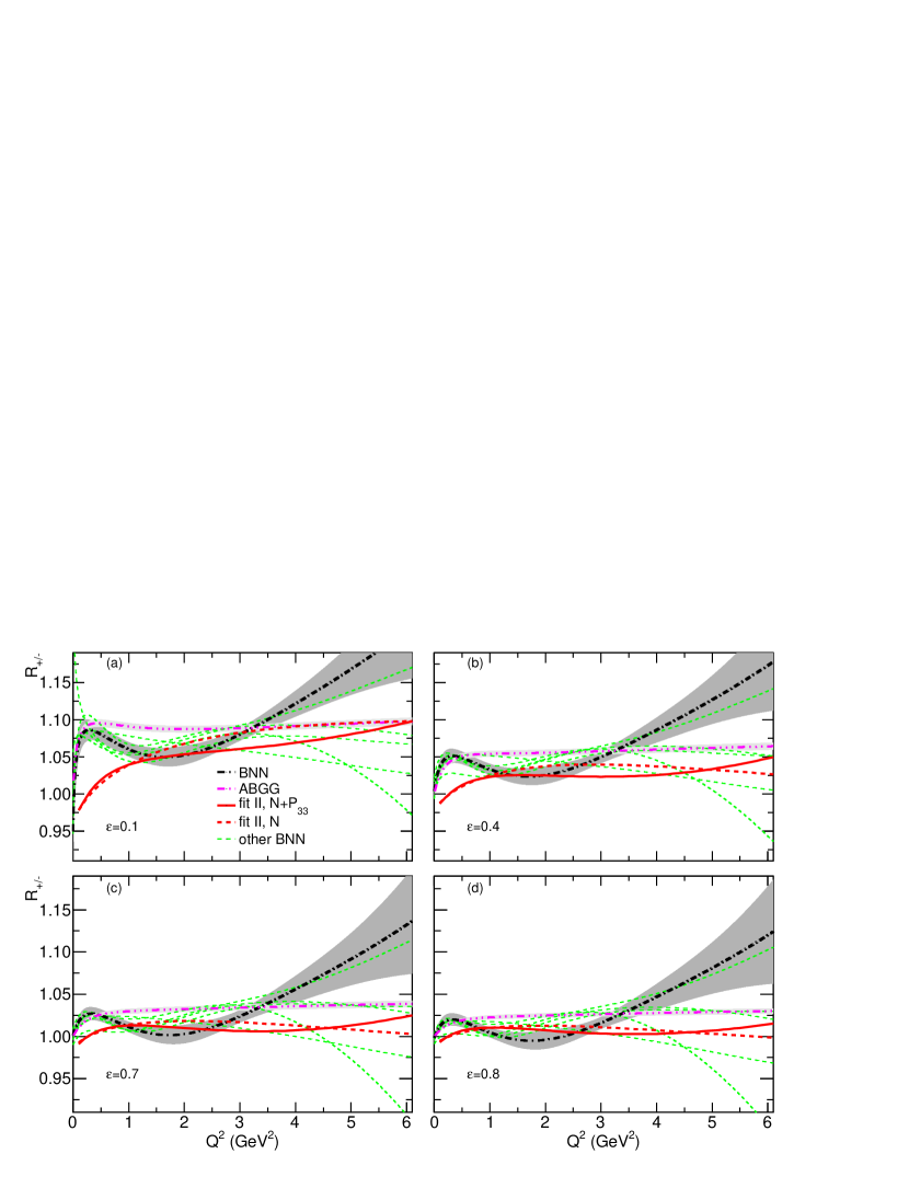
Figure 10: (Color online) Predictions of $R_{+/-}$ (Eq. 2) computed based on the BNN, HM (fit II) and ABGG approaches. The TPE correction includes either elastic $(N)$ or elastic and $P_{33}$ resonance (full model) contributions. Additionally the plots of $R_{+/-}$ predicted based on the BNN fits rejected due too small value of the evidence (see Tab. 3), are presented (other BNN). The shaded areas show $1\sigma$ error computed from the covariance matrix.

V Neural Network vs. Hadronic Model

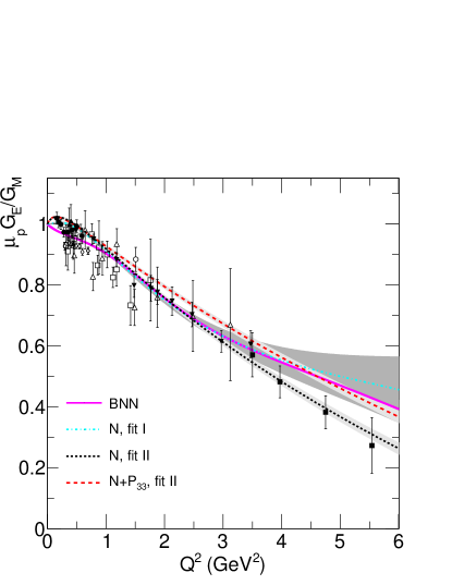
Figure 11: (Color online) Ratio $\mu_{p}G_{E}/G_{M}$ computed based on the fits I and II as well as for BNN. The HM fits include either elastic $(N)$ or elastic and $P_{33}$ resonance contributions. The PT data are taken from Refs. PT_data ; Zhan:2011ji . The shaded areas show $1\sigma$ error computed from the covariance matrix.

	$k=1$	$k=2$
$m_{1}^{k}$	$1.234$	$0.321$
$m_{2}^{k}$	$0.181$	$4.298$
$m_{3}^{k}$	$1.085$	$4.641$
$f_{1}^{k}$	$-6.569$	$0.694$
$f_{2}^{k}$	$0.055$	$-13.44$

	$k=1$	$k=2$
$m_{1}^{k}$	$1.221$	$0.327$
$m_{2}^{k}$	$0.173$	$4.019$
$m_{3}^{k}$	$1.097$	$4.450$
$f_{1}^{k}$	$-7.934$	$0.713$
$f_{2}^{k}$	$0.051$	$-10.16$

Table 1: Form factor parameters for the fit I (56) for the hadronic model with elastic (N) (left panel) and elastic and resonance $P_{33}$ (right panel) TPE contributions. Mass parameters are in the units of $GeV$.

The electromagnetic FFs of the proton are the input of the hadronic model used in this paper. For the comparison self-consistency the proton FFs of HM are obtained from the fit of HM to the same unpolarized cross section data as in the BNN (for details see Appendix B). The PT and $R_{+/-}$ data are not taken into consideration, and the constraint coming from the assumption (A) does not affect the results. The TPE correction contains either $\Box(N)$ or $\Box(N+P_{33})$ contributions. The obtained FFs parameters are given in Tables. 1 (fit I) and 2 (fit II), while the values of $\chi^{2}_{min}/NDF$ (NDF = number degrees of freedom) are reported in the table below.

FF	$(N)$	$(N+P_{33})$
fit I	$389/403$	$397/403$
fit II	$386/403$	$395/403$

It is interesting to notice that the mass parameters of the fit I are not well-spaced. For instance the parameters $m_{1}^{1}$ and $m_{3}^{1}$ take quite similar values. The same feature characterizes the fits from Ref. Blunden:2005ew , where the parametrization I was also discussed but it was fitted to the FFs from Ref. Mergell:1995bf . Indeed, this parametrization at large $Q^{2}$ behaves as $1/Q^{2}$, while it is expected (based on the theoretical arguments Kelly:2004hm ; Brodsky:1973kr ) that $G_{E,M}\sim 1/Q^{4}$.

The above observations may suggest that the parametrization I is too simple to describe accurately the FFs in the wide $Q^{2}$ range. In order to verify this statement we make two fits. In the first we consider the data below $Q^{2}=$ 1 GeV², while in the other we use the data below $Q^{2}=0.5$ GeV². For the first case we get the mass parameters $m_{1}^{1}=2.59$, $m_{2}^{1}=0.95$ and $m_{3}^{1}=0.18$ and for the other $m_{1}^{1}=1.70$, $m_{2}^{1}=0.21$ and $m_{3}^{1}=9.16$. We see that for low $Q^{2}$-data fits the mass parameters are well separated. However, because the problems remarked above in further discussion the HM with the FFs given by fit I is treated as a toy model, discussed to present the systematic properties of the hadronic approach.

	$k=1$	$k=2$
$m_{1}^{k}$	$0.7732$	$1.0595$
$m_{2}^{k}$	$0.9489$	$1.5629$
$m_{3}^{k}$	$0.8457$	$0.5474$
$f_{1}^{k}$	$3.9833$	$1.2645$
$f_{2}^{k}$	$3.9334$	$-0.269$

	$k=1$	$k=2$
$m_{1}^{k}$	$0.7866$	$1.0247$
$m_{2}^{k}$	$0.9641$	$1.4914$
$m_{3}^{k}$	$0.8550$	$0.5082$
$f_{1}^{k}$	$4.3360$	$1.4592$
$f_{2}^{k}$	$3.7328$	$-0.3175$

Table 2: Form factor parameters for the fit II (• ‣ IV.2) for the hadronic model with elastic (N) (left panel) and elastic and resonance $P_{33}$ (right panel) TPE contributions. Mass parameters are in the units of GeV.

At low-$Q^{2}$ there is a visible discrepancy between the BNN and the hadronic model FFs fits. It is illustrated in Fig. 9, where the ratio $\mu_{p}G_{E}/G_{M}$ is plotted. There is a satisfactory agreement between the fits I and II. On the contrary the ratio $\mu_{p}G_{E}/G_{M}$ predicted by the BNN approach is more consistent with the recent PT measurements Zhan:2011ji (these data were not included in the BNN fit).

The low-$Q^{2}$ discrepancy between HM and BNN approaches is the result of different treatment of the TPE corrections. It is illustrated in Fig. 7 where we plot the function,

$$D_{2\gamma}=\frac{\Delta_{2\gamma}}{1+\Delta_{2\gamma}}=\frac{\Delta C_{2\gamma}}{\sigma_{R,1\gamma+2\gamma}}.$$ (64)

It can be seen that the BNN and HM predictions are inconsistent for $Q^{2}\in(0.02,1)$ GeV². On the contrary, below $Q^{2}<0.02$ GeV² and at low $\varepsilon$ there is a good agreement between TPE predictions obtained within both methodologies as well as other theoretical calculations Coulomb_distortion . This low $\varepsilon$ and $Q^{2}$ behaviour of the BNN fit seems to be a systematic property of all BNN-based parametrizations. It is illustrated in Fig. 12, where the $R_{+/-}$ predicted by the BNN models, rejected due to too small value of the evidence (see Table 3), are plotted. In the limit of $\varepsilon\to 0$, with $Q^{2}$ very low but fixed, $\sigma_{R,1\gamma}$ (Eq. 10) is dominated by the magnetic contribution, and the main constraint comes from the fact that $G_{M}(Q^{2}=0)=\mu_{p}$. As the result the TPE fit is affected by several data points present at low $Q^{2}$ and $\varepsilon$ domain.

For completeness of the low-$Q^{2}$ comparison we report the values of the proton radius obtained from the BNN and HM fits.

	BNN	fit I	fit II
$\sqrt{\langle r^{2}_{E}\rangle}$ (fm)	$0.85\pm 0.01$	$0.898\pm 0.001$	$0.867\pm 0.002$

The value of $\sqrt{\langle r^{2}_{E}\rangle}$ computed from the BNN fit is consistent with the fit II and the recent atomic measurement Pohl:2010zza (0.84087(39) fm). However, it disagrees with the prediction based on the fit I. The latter is inconsistent with the fit II as well.

There are two major reasons for the above inconsistency. The first one is induced by the systematic differences between the predictions of the TPE by BNN and HM approaches in the low $Q^{2}$ range. The discrepancy between the values of the proton radius based on the fits I and II is the result of the problems of parametrization I (mentioned already above) with the proper description of the FFs in the wide $Q^{2}$ range. In general the low number of parameters in fits I and II limits the flexibility of the FF parametrizations and their ability for simultaneous description of the low and high $Q^{2}$ data. Therefore the low/high $Q^{2}$ fit dependence can be affected by the high/low $Q^{2}$ data.

To summarize, the low-$Q^{2}$ discussion we would like to emphasize that in both the present and the BNN data analyses our attention was not particularly focused on the $Q^{2}\to 0$ limit. Certainly, accurate calculations of the proton radius require more careful discussion, as it is reported in Refs. Arrington:2006hm ; Zhan:2011ji ; Bernauer:2010wm ; Arrington:2011kv ; Arrington:2012dq ; Pohl:2013yb .

Above $Q^{2}=1$ GeV² the BNN FFs ratio $\mu_{p}G_{E}/G_{M}$, on the qualitative level, is comparable with the hadronic model predictions (Fig. 11). All fits agree well with the PT measurements PT_data . As it could be expected the inclusion into the hadronic model of the $\Box(P_{33})$ contribution increases the value of the electric form factor at larger values of $Q^{2}$ (see Fig. 11).

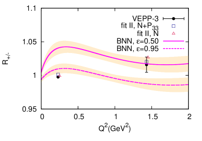
Figure 12: (Color online) The ratio $R_{+/-}$ computed based on the BNN (lines) and HM (squares and triangles) approaches as well as the preliminary VEPP-3 measurements Gramolin:2011tr (filled circles). The HM predictions are computed for the model (fit II) which contains either elastic $(N)$ or elastic and resonance $P_{33}$ TPE contributions. The triangle points are right shifted by 0.02 GeV². The shaded areas show $1\sigma$ error computed from the covariance matrix.

An excellent consistency between predictions of the TPE effect by the BNN and HM approaches appears for $Q^{2}\in(1,3)$ GeV² (Figs. 10 as well as 7 and 8). Above $Q^{2}=3$ GeV² the agreement is on the $2\sigma$ level only.

In order to show the strength of the BNN approach we confront its predictions of the TPE effect with our previous global analysis (ABGG) Alberico:2008sz made in the conventional way (see Figs. 7 and 8). In this approach, following the proposal of Ref. Chen:2007ac , some functional form of the TPE term was postulated. But the same cross section and the PT data, as in the case of the BNN were analysed. The constraint (A) was also imposed. Although both the electric and the magnetic FF fits of ABGG analysis are very similar to those obtained within the BNN and the other phenomenological approaches Qattan:2011ke , the predictions of the TPE correction agree with the HM only for $Q^{2}$ around 3 GeV² (see Fig. 10). In the ABGG approach the model-dependence of the final fits was not discussed. The successful fits were characterized by reasonable value of $\chi^{2}_{min}/NDF$. However, in the BNN analysis the models rejected, due too low evidence, were characterized also by the reasonable $\chi^{2}_{min}/NDF$ (see Table 3). But the TPE corrections predicted based on these fits, similarly as for ABGG are inconsistent with the best BNN fit and the hadronic model calculations.

	$\mathcal{N}_{4,2}$	$\mathcal{N}_{4,3}$	$\mathcal{N}_{6,2}$	$\mathcal{N}_{6,3}$	$\mathcal{N}_{6,4}$	$\mathcal{N}_{5,7}$	$\mathcal{N}_{5,6}$
$\chi^{2}_{min}$	$507$	$511$	$497$	$493$	$486$	$539$	$\mathbf{478}$
ln(evidence)	$-633$	$-630$	$-635$	$-624$	$-639$	$-699$	$\mathbf{-611}$

Table 3: The minimum of $\chi^{2}$ and the maximum of the evidence obtained for the best BNN model (bold fonts) and the fits rejected because of too small value of the evidence. A total number of points in the fit is 529.

The results of this paper are complementary to the conclusions of Ref. Arrington:2007ux (AMT). In this paper the global analysis of the world $ep$ data was performed. The TPE correction was given by a sum of the elastic $\Box(N)$ and inelastic contributions. The latter was described by a phenomenological function, which approximates the resonance Kondratyuk:2006ig and GPD-based Afanasev:2005mp fraction of the TPE effect. To compute the elastic contribution the FFs (parametrization I) were fitted to the electromagnetic FFs from Mergell:1995bf . The FFs (parametrization from Kelly:2004hm ) were fitted to the unpolarized cross section data (corrected by the TPE) and the PT measurements. It was shown that the cross section data modified due to the TPE effect are consistent with the PT measurements. An effort was made to estimate uncertainties of the theoretical model for the TPE effect.

In the AMT as well as in the ABGG approaches the analyses were performed in the spirit of frequentis statistics (using the least square method), while the neural network analysis was done within the Bayesian statistics (for the short review see PDG ). In both statistical approaches to find the best fit some error function is minimized. But in the BNN approach the procedure of finding the optimal model is more complicated. In the first stage of the approach the large population of the MLPs (more than 1000 of networks of given architectures) is trained to find the configuration of the weight parameters for which the error function is at the local minimum. The best model, favoured by the data, maximizes the evidence. It is the probability distribution, which only partially depends on the error function. It contains the Occam’ contribution (Eqs. LABEL:evidence_Occam_volume and 35), which penalizes too complex models and allows one to choose the fit with the best predictive power.

The idea of the BNN formalism is to distinguish the statistical model, describing the data, which is characterized by good predictive power. To verify this property we make an estimate of $R_{+/-}$ for the new measurements done by VEPP-3 experiment Gramolin:2011tr , which were not included in the BNN analysis. It can be noticed that the BNN and the HM predictions are consistent with the new data (see Fig. 12). For the future tests we provide reader with our predictions of $R_{+/-}$ for two other kinematics, which are going to be explored by the Novosibirsk experiment, see Table 4.

$Q^{2}$(GeV2)	$0.23$	$1.43$	$0.82$	$0.96$
$\varepsilon$	$0.95$	$0.50$	$0.42$	$0.29$
	$1.009$	$1.017$	$1.037$	$1.043$
BNN	$\pm 0.007$	$\pm 0.010$	$\pm 0.007$	$\pm 0.008$
$\Box(N)$	0.999	1.026	1.020	1.028
$\Box(N+P_{33})$	1.001	1.020	1.019	1.027

Table 4: $R_{+/-}$ predictions for VEPP-3 experiment Gramolin:2011tr computed within the BNN and HM approaches. In the latter the model contains either elastic $(N)$ or elastic and resonance $P_{33}$ TPE contributions (fit II).

VI Summary

The TPE correction was computed within the hadronic model. For the hadronic intermediate states the proton and $P_{33}(1232)$ resonance were considered. The electromagnetic proton form factor parameters were obtained from the global fit to the cross section data only. Two FF parametrizations were discussed, the sum of monopoles and dipoles. The TPE $\Box(P_{33})$ contribution was computed taking different form of transition vertex and form factors than discussed previously. In particular two parametrizations of the FFs for the $N\to P_{33}$ were considered.

The main goal of this paper was to confront the predictions of the TPE effect coming from the hadronic model and the Bayesian analysis of the $ep$ scattering data. The latter was preformed by applying the neural network framework. The BNN response was constrained by the assumption that the PT data is not sensitive to TPE effect. Hence this comparison provides also a quantitative verification of this assumption.

It was demonstrated that the BNN and the hadronic model predictions agree on quantitative level in a wide $Q^{2}$ range. In particular for $Q^{2}$ between $1$ GeV² and $3$ GeV² the TPE corrections resulting form both approaches are very similar. In the intermediate $Q^{2}$ range ($Q^{2}>3$ GeV²) the agreement is on $2\sigma$ level. It is the kinematical domain where the data is limited. Obviously it affects the BNN predictions. On the other hand in this kinematical limit the applied hadronic model can be questionable.

For $Q^{2}$ between $0.01$ GeV² and $0.8$ GeV² the BNN and hadronic model predictions are inconsistent. In this $Q^{2}$ range the assumption (A) does not work effectively. Similar inconsistency appears when one compares with the ABGG predictions of the TPE. Indeed, in the ABGG approach the assumption (A) also played a crucial role in the analysis.

A next step to improve the BNN approach would be to replace the assumption (A) by a weaker statement, and enlarge the number of independent TPE functions from one to six. The main problem is that the PT data seems to be not informative enough about $\varepsilon$ dependence of the TPE effect.

Appendix A Evaluation of TPE Term

We consider the proton electromagnetic FFs of the form,

$$F_{i}(t)=\sum_{k=1}^{L_{i}}\sum_{n_{k}^{i}=1}^{N_{k}^{i}}\frac{f^{n_{k}^{i}}_{i}}{(t-M_{i,n_{k}}^{2})^{k}},i=1,2.$$ (65)

Every $k-th$ pole function can be written as a derivative,

$$\frac{1}{(n-1)!}\left.\partial_{x}^{n-1}\frac{1}{t-x}\right|_{x=M^{2}}=\frac{1}{(t-M^{2})^{n}}$$ (66)

We introduce a notation,

$$\mathcal{D}^{n}_{M}f(M^{2})\equiv\frac{1}{(n-1)!}\left.\frac{\partial^{n}f(x^{2})}{\partial(x^{2})^{n}}\right|_{x^{2}=M^{2}},\;\;n=1,2,...,$$ (67)

where $\mathcal{D}^{0}_{M}f(M^{2})\equiv f(M^{2}).$ Then the form factor is written in the form,

$$F_{i}(t)=\sum_{k=1}^{L_{i}}\sum_{n_{k}^{i}=1}^{N_{k}^{i}}\mathcal{D}_{M_{n_{k}^{i}}}^{k-1}\frac{f^{n_{k}^{i}}_{i}}{t-M_{n_{k}^{i}}^{2}}.$$ (68)

We decompose both $w_{N,\parallel}$ and $w_{N,\times}$ functions into four components,

$$w_{N}=\sum_{i=1}^{2}\sum^{2}_{j=1}w^{ij}_{N}.$$ (69)

The $ij$ component, due to its form factor, reads

$$w^{ij}_{N}=\sum_{k=1}^{L_{i}}\sum_{n_{k}^{i}=1}^{N_{k}^{i}}\sum_{l=1}^{L_{j}}\sum_{n_{l}^{j}=1}^{N_{l}^{j}}f^{n_{k}^{i}}_{i}f^{n_{l}^{j}}_{j}\mathcal{D}_{M_{n_{k}^{i}}}^{k-1}\mathcal{D}_{M_{n_{l}^{j}}}^{l-1}\mathcal{E}(L^{\alpha\mu\nu}\mathcal{H}^{N,ij}_{\alpha\mu\nu},M_{n_{k}^{i}},M_{n_{l}^{j}},M_{p}),$$ (70)

where the leptonic tensor $L^{\alpha\mu\nu}$ is given by either

$$L^{\alpha\mu\nu}_{\parallel}=\mathrm{Tr}\left((\hat{k}+m)\gamma^{\alpha}(\hat{k^{\prime}}+m)\gamma^{\mu}(\hat{k^{\prime}}-\hat{l}+m)\gamma^{\nu}\right)$$ (71)

or

$$L^{\alpha\mu\nu}_{\times}=\mathrm{Tr}\left((\hat{k}+m)\gamma^{\alpha}(\hat{k^{\prime}}+m)\gamma^{\mu}(\hat{k^{\prime}}-\hat{l}+m)\gamma^{\nu}\right).$$ (72)

The hadronic tensor reads,

$$\mathcal{H}^{N,ij}_{\alpha\mu\nu}=\mathrm{Tr}\left((\hat{p}+M_{p})\Gamma_{\alpha}(-q)(\hat{p^{\prime}}+M_{p})\Gamma_{\mu}^{i}(-l)(\hat{p^{\prime}}+\hat{l}+M_{p})\Gamma_{\nu}^{j}(q+l)\right),$$ (73)

$$\Gamma^{1}_{\mu}(l)\equiv\gamma_{\mu},\quad\Gamma^{2}_{\mu}(l)=\frac{i\sigma^{\mu\nu}l_{\nu}}{2M_{p}}.$$ (74)

$\mathcal{E}(\mathcal{N},m_{a},m_{b},m_{h})$ is the one-loop integral defined as,

$$\mathcal{E}_{\parallel}(\mathcal{N},m_{a},m_{b},m_{h})=\int\frac{d^{4}l}{(2\pi)^{4}}\frac{\mathcal{N}}{[l^{2}-m_{a}^{2}][(q+l)^{2}-m_{b}^{2}][(q+l)^{2}+i\epsilon][l^{2}+i\epsilon][(k^{\prime}-l)^{2}-m^{2}+i\epsilon][(p^{\prime}+l)^{2}-m^{2}_{h}+i\epsilon]}$$ (75)

for direct box diagram, and

$$\mathcal{E}_{\times}(\mathcal{N},m_{a},m_{b},m_{h})=\int\frac{d^{4}l}{(2\pi)^{4}}\frac{\mathcal{N}}{\left[l^{2}-m_{a}^{2}\right]\left[(q+l)^{2}-m_{b}^{2}\right]\left[(q+l)^{2}+i\epsilon\right]\left[l^{2}+i\epsilon\right][(k+l)^{2}-m^{2}+i\epsilon][(p^{\prime}+l)^{2}-m^{2}_{h}+i\epsilon]}$$ (76)

for exchange box diagram.

In the case of the $P_{33}$ intermediate state we proceed in the similar manner. For instance for the $P_{33}(Full)$ model we have

$$w_{\Delta}=\sum_{i=1}^{3}\sum^{3}_{j=1}w^{ij}_{\Delta}.$$ (77)

The components of hadronic tensor read,

$$\mathcal{H}^{\Delta,ij}_{\alpha\mu\nu}=\mathrm{Tr}\left((\hat{p}+M_{p})\Gamma_{\alpha}(-q)(\hat{p^{\prime}}+M_{p})\Gamma_{\mu\xi,i}^{\Delta,in}(-l,p^{\prime}+l)\left[\hat{p^{\prime}}+\hat{l}+M_{\Delta}\right]\Lambda^{\xi\eta}(p^{\prime}+l)\Gamma_{\eta\nu,j}^{\Delta,out}(q+l,p^{\prime}+l)\right),$$ (78)

where

$$\Gamma_{\mu\nu,i}^{\Delta,in(out)}\equiv\Gamma_{\mu\nu}^{\Delta,in(out)}(C_{k}^{V}\to\delta_{ki},k=3,4,5)$$ (79)

In the case of $P_{33}(full)$ model for the resonance form factors have a general form,

$$C_{i}^{V}(t)=-c_{i}^{V}\frac{a_{i}M_{V}^{2}}{t-a_{i}M_{V}^{2}}\frac{M_{V}^{4}}{(t-M_{V}^{2})^{2}}.$$ (80)

They can be written in the form,

$$C_{i}^{V}(t)=\frac{c_{i}^{1,1}}{\left[t-(M_{i}^{1,1})^{2}\right]^{2}}+\frac{c_{i}^{1,2}}{\left[t-(M_{i}^{1,2})^{2}\right]}+\frac{c_{i}^{2,1}}{\left[t-(M_{i}^{2,1})^{2}\right]^{2}},$$ (81)

where

$$C_{i}^{1,1} = -c_{i}^{V}\frac{a_{i}M_{V}^{2}}{(a_{i}-1)^{2}},\quad M_{i}^{1,1}=\sqrt{a_{i}}M_{V},$$ (82)

$$C_{i}^{1,2} = c_{i}^{V}\frac{a_{i}M_{V}^{2}}{(a_{i}-1)^{2}},\quad M_{i}^{1,1}=M_{V}$$ (83)

$$C_{i}^{2,1} = c_{i}^{V}\frac{a_{i}M_{V}^{4}}{(a_{i}-1)},\quad M_{i}^{1,1}=M_{V}.$$ (84)

$$w^{ij}_{\Delta}=\sum_{k=1}^{2}\sum_{n_{k}=1}^{N_{k}}\sum_{l=1}^{2}\sum_{n_{l}=1}^{N_{l}}c^{k,n_{k}}_{i}c^{l,n_{l}}_{j}\mathcal{D}_{M_{i}^{k,n_{k}}}^{k-1}\mathcal{D}_{M_{j}^{l,n_{l}}}^{l-1}\mathcal{I}(L^{\alpha\mu\nu}\mathcal{H}^{\Delta,ij}_{\alpha\mu\nu},M_{i}^{k,n_{k}},M_{j}^{l,n_{l}},M_{\Delta}),$$ (85)

where $N_{1}=2$, $N_{2}=1$.

The algebraical calculations, like computing the leptonic (71), (72) and hadronic (73), (78) tensors and their contractions, are done with help of FeynCalc package Mertig:1990an ; Mertig:1998vk .

The integrals (75), (76) are expressed (also with the help of routines in FeynCalc) in terms of Veltman-Passariono scalar loop integrals tHooft_1979 Passarino79 . Because of the complex structure of the the numerators of the integrals (75), (76) some pre-reduction the numerator with the denominator is necessary.

Having the analytic expressions for all integral components, their numerical values are computed with LoopTool library vanOldenborgh:1989wn ; Hahn:1998yk .

Appendix B $\chi^{2}$

In order to get the FFs parameters of the parametrization I (56) and II (• ‣ IV.2) we analyse the same unpolarized cross section data as in Ref. Graczyk:2011kh .

We consider the following $\chi^{2}$ function,

$$\chi^{2}=\sum_{k=1}^{N}\left[\sum_{i=1}^{n_{k}}\left(\frac{\lambda_{k}\sigma^{th}_{ki}-\sigma^{ex}_{ki}}{\Delta\sigma_{ki}}\right)^{2}+\left(\frac{\lambda_{k}-1}{\Delta\lambda_{k}}\right)^{2}\right].$$ (86)

$N=28$ is a number of independent data sets in the fit; $n_{k}$ is a number of points in the $k$-th data set; $\sigma_{ki}^{th}$ is the reduced cross section given by Eq. (16), while $\sigma^{ex}_{ki}$ and $\Delta\sigma^{ex}_{ki}$ denote the experimental measurement and its error. By $\Delta\lambda_{k}$’s the systematic normalization errors are introduced. For every data set the normalization parameter $\lambda_{k}$ is established from the fit. A treatment of the systematic normalization errors is the same as in Refs. Arrington:2003df ; Alberico:2008sz ; Graczyk:2011kh ; Arrington:2007ux . For the statistical explanation of this procedure see Ref. D'Agostini:1995fv .

References

- (1) G. Ron et al., Phys. Rev. C 84 (2011) 055204. A. J. R. Puckett, E. J. Brash, O. Gayou, M. K. Jones, L. Pentchev, C. F. Perdrisat, V. Punjabi and K. A. Aniol et al., Phys. Rev. C 85 (2012) 045203.
- (2) P. G. Blunden, W. Melnitchouk and J. A. Tjon, Phys. Rev. Lett. 91 (2003) 142304.
- (3) P. A. M. Guichon and M. Vanderhaeghen, Phys. Rev. Lett. 91 (2003) 142303.
- (4) Y. C. Chen, A. Afanasev, S. J. Brodsky, C. E. Carlson and M. Vanderhaeghen, Phys. Rev. Lett. 93 (2004) 122301.
- (5) Y. -S. Tsai, Phys. Rev. 122 (1961) 1898; L. W. Mo and Y. S. Tsai, Rev. Mod. Phys. 41 (1969) 205; Y. -S. Tsai, Radiative Corrections To Electron Scatterings, Lectures given at NATO Advanced Institute on Electron Scattering and Nuclear Structure at Cagliari, Italy, September 1970, SLAC-PUB-0848.
- (6) Y. .M. Bystritskiy, E. A. Kuraev and E. Tomasi-Gustafsson, Phys. Rev. C 75 (2007) 015207.
- (7) P. G. Blunden, W. Melnitchouk and J. A. Tjon, Phys. Rev. C 72 (2005) 034612.
- (8) H. Q. Zhou, C. W. Kao, S. N. Yang and K. Nagata, Phys. Rev. C 81 (2010) 035208.
- (9) S. Kondratyuk, P. G. Blunden, W. Melnitchouk and J. A. Tjon, Phys. Rev. Lett. 95 (2005) 172503.
- (10) S. Kondratyuk and P. G. Blunden, Nucl. Phys. A 778 (2006) 44.
- (11) D. Borisyuk and A. Kobushkin, Phys. Rev. C 74 (2006) 065203.
- (12) D. Borisyuk and A. Kobushkin, Phys. Rev. C 78 (2008) 025208.
- (13) D. Borisyuk and A. Kobushkin, Phys. Rev. C 86 (2012) 055204.
- (14) A. V. Afanasev, S. J. Brodsky, C. E. Carlson, Y. -C. Chen and M. Vanderhaeghen, Phys. Rev. D 72 (2005) 013008.
- (15) D. Borisyuk and A. Kobushkin, Phys. Rev. D 79 (2009) 034001.
- (16) J. A. Tjon, P. G. Blunden and W. Melnitchouk, Phys. Rev. C 79 (2009) 055201.
- (17) N. Kivel and M. Vanderhaeghen, JHEP 1304 (2013) 029.
- (18) D. Borisyuk and A. Kobushkin, Two photon exchange amplitude with intermediate states: P33 channel, arXiv:1306.4951 [hep-ph].
- (19) J. Arrington, P. G. Blunden and W. Melnitchouk, Prog. Part. Nucl. Phys. 66 (2011) 782.
- (20) M. Vanderhaeghen, Few Body Syst. 41 (2007) 103.
- (21) C. E. Carlson and M. Vanderhaeghen, Ann. Rev. Nucl. Part. Sci. 57 (2007) 171.
- (22) J. Arrington, Phys. Rev. C 69 (2004) 022201.
- (23) E. Tomasi-Gustafsson and G. I. Gakh, Phys. Rev. C 72 (2005) 015209.
- (24) V. Tvaskis, J. Arrington, M. E. Christy, R. Ent, C. E. Keppel, Y. Liang and G. Vittorini, Phys. Rev. C 73 (2006) 025206.
- (25) M. A. Belushkin, H. -W. Hammer and U. -G. Meissner, Phys. Lett. B 658 (2008) 138.
- (26) D. Borisyuk and A. Kobushkin, Phys. Rev. C 76 (2007) 022201.
- (27) J. Arrington, W. Melnitchouk and J. A. Tjon, Phys. Rev. C 76 (2007) 035205.
- (28) Y. C. Chen, C. W. Kao and S. N. Yang, Phys. Lett. B 652 (2007) 269.
- (29) W. M. Alberico, S. M. Bilenky, C. Giunti and K. M. Graczyk, Phys. Rev. C 79 (2009) 065204.
- (30) E. Tomasi-Gustafsson, M. Osipenko, E. A. Kuraev, Y. .Bystritsky and V. V. Bytev, Compilation and analysis of charge asymmetry measurements from electron and positron scattering on nucleon and nuclei, arXiv:0909.4736 [hep-ph].
- (31) J. Guttmann, N. Kivel, M. Meziane and M. Vanderhaeghen, Eur. Phys. J. A 47 (2011) 77.
- (32) S. Venkat, J. Arrington, G. A. Miller and X. Zhan, Phys. Rev. C 83 (2011) 015203.
- (33) K. M. Graczyk, Phys. Rev. C 84 (2011) 034314.
- (34) I. A. Qattan, A. Alsaad and J. Arrington, Phys. Rev. C 84 (2011) 054317.
- (35) I. A. Qattan and A. Alsaad, Phys. Rev. C 83 (2011) 054307 [Erratum-ibid. C 84 (2011) 029905].
- (36) R. P. Bennett, AIP Conf. Proc. 1441 (2012) 156.
- (37) A. V. Gramolin, J. Arrington, L. M. Barkov, V. F. Dmitriev, V. V. Gauzshtein, R. A. Golovin, R. J. Holt and V. V. Kaminsky et al., Nucl. Phys. Proc. Suppl. 225-227 (2012) 216.
- (38) L. Ice et al. [OLYMPUS Collaboration], AIP Conf. Proc. 1423 (2012) 206.
- (39) K. M. Graczyk, P. Plonski and R. Sulej, JHEP 1009 (2010) 053.
- (40) M. P. Rekalo and E. Tomasi-Gustafsson, Eur. Phys. J. A 22 (2004) 331.
- (41) M. P. Rekalo and E. Tomasi-Gustafsson, Nucl. Phys. A 740 (2004) 271.
- (42) M. P. Rekalo and E. Tomasi-Gustafsson, Nucl. Phys. A 742 (2004) 322.
- (43) R. Pohl, A. Antognini, F. Nez, F. D. Amaro, F. Biraben, J. M. R. Cardoso, D. S. Covita and A. Dax et al., Nature 466 (2010) 213.
- (44) L. C. Maximon and J. A. Tjon, Phys. Rev. C 62 (2000) 054320
- (45) H. W. L. Naus and J. H. Koch, Phys. Rev. C 36 (1987) 2459. P. C. Tiemeijer and J. A. Tjon, Phys. Rev. C 42 (1990) 599.
- (46) B. Denby, Computer Physics Communications 49 (1988), 429; Mellado B. et al., Phys. Lett. B611 (2005), 60. K. Kurek, E. Rondio, R. Sulej, K. Zaremba, Meas. Sci. Technol. 18 (2007) 2486. J. Damgov and L. Litov, Nucl. Inst. Meth. A482 (2002) 776. T. Bayram, S. Akkoyun and S. O. Kara, Annals of Nuclear Energy, 63 (2014) 172. S. Akkoyun, T. Bayram, S. O. Kara and A. Sinan, J. Phys. G 40 (2013) 055106.
- (47) J. Hertz, A. Krogh, R. G. Palmer, Introduction to the Theory of Neural Computation, Santa Fe Institute Studies in the Sciences of Complexity, Westview Press 1991.
- (48) R. D. Ball et al. [The NNPDF Collaboration], Nucl. Phys. B 874 (2013) 36.
- (49) G. Cybenko, Math. Control Signals System (1989) 2, 303.
- (50) C. M. Bishop, Neural Networks for Pattern Recognition, Oxford University Press 2008.
- (51) D. J. C. MacKay, Neural Computation 4 (3), (1992) 415; D. J. C. MacKay, Neural Computation 4 (3), (1992) 448; D. J. C. MacKay, Bayesian methods for backpropagation networks, in E. Domany, J. L. van Hemmen, and K. Schulten (Eds.), Models of Neural Networks III, Sec. 6. New York: Springer-Verlag (1994).
- (52) D. J.C. MacKay, California Institute of Technology, Pasadena, California, December 10, 1991, Bayesian Methods for Adaptive Models, http://www.inference.phy.cam.ac.uk/mackay/PhD.html.
- (53) T. Pospischil et al. [A1 Collaboration], Eur. Phys. J. A 12 (2001) 125. O. Gayou et al., Phys. Rev. C 64 (2001) 038202. O. Gayou et al. [Jefferson Lab Hall A Collaboration], Phys. Rev. Lett. 88 (2002) 092301. V. Punjabi et al., Phys. Rev. C 71 (2005) 055202 [Erratum-ibid. C 71 (2005) 069902]. C. B. Crawford et al., Phys. Rev. Lett. 98 (2007) 052301. M. K. Jones et al. [Resonance Spin Structure Collaboration], Phys. Rev. C 74 (2006) 035201.
- (54) X. Zhan, K. Allada, D. S. Armstrong, J. Arrington, W. Bertozzi, W. Boeglin, J. -P. Chen and K. Chirapatpimol et al., Phys. Lett. B 705 (2011) 59.
- (55) H. F. Jones and M. D. Scadron, Annals Phys. 81 (1973) 1.
- (56) J. Liu, N. C. Mukhopadhyay and L. s. Zhang, Phys. Rev. C 52 (1995) 1630.
- (57) L. Alvarez-Ruso, S. K. Singh and M. J. Vicente Vacas, Phys. Rev. C 59 (1999) 3386.
- (58) O. Lalakulich, E. A. Paschos and G. Piranishvili, Phys. Rev. D 74 (2006) 014009.
- (59) D. Drechsel, S. S. Kamalov and L. Tiator, Eur. Phys. J. A 34 (2007) 69.
- (60) P. Mergell, U. G. Meissner and D. Drechsel, Nucl. Phys. A 596 (1996) 367.
- (61) J. J. Kelly, Phys. Rev. C 70 (2004) 068202.
- (62) S. J. Brodsky and G. R. Farrar, Phys. Rev. Lett. 31 (1973) 1153.
- (63) W. A. McKinley and H. Feshbach, Phys. Rev. 74 (1948) 1759. R. H. Dalitz, Proc. R. Soc. Lond. A206, 509 (1951), Proc. R. Soc. Lond. A206, 521 (1951).
- (64) J. Arrington, J. Phys. G 40 (2013) 115003.
- (65) J. C. Bernauer et al. [A1 Collaboration], Phys. Rev. Lett. 105 (2010) 242001.
- (66) J. Arrington and I. Sick, Phys. Rev. C 76 (2007) 035201.
- (67) J. Arrington, Phys. Rev. Lett. 107 (2011) 119101.
- (68) R. Pohl, R. Gilman, G. A. Miller and K. Pachucki, Ann. Rev. Nucl. Part. Sci. 63 (2013) 175.
- (69) Statistics, by G. Cowan (RHUL) in J. Beringer et al. (PDG), Physical Review D86, 010001 (2012) (http://pdg.lbl.gov). G. D’Agostini, Bayesian reasoning in data analysis: a critical introduction, World Scientific 2003.
- (70) Wroclaw Centre for Networking and Supercomputing, http://www.wcss.pl/en/
- (71) R. Mertig, M. Bohm and A. Denner, Comput. Phys. Commun. 64 (1991) 345.
- (72) R. Mertig and R. Scharf, Comput. Phys. Commun. 111 (1998) 265 [hep-ph/9801383].
- (73) G. ’t Hooft, and M. Veltman, Nucl. Phys. B153 (1979) 365.
- (74) G. Passariono, M. Veltman, Nucl. Phys. B160 (1979) 151.
- (75) G. J. van Oldenborgh and J. A. M. Vermaseren, Z. Phys. C 46 (1990) 425.
- (76) T. Hahn and M. Perez-Victoria, Comput. Phys. Commun. 118 (1999) 153
- (77) J. Arrington, Phys. Rev. C 68 (2003) 034325.
- (78) G. D’Agostini, Probability and measurement uncertainty in physics: A Bayesian primer, hep-ph/9512295.